Article

Symmetry-Enhanced, Improved Pathfinder Algorithm-Based Multi-Strategy Fusion for Engineering Optimization Problems

School of Mathematical Sciences, Mudanjiang Normal University, Mudanjiang 157000, China
*
Author to whom correspondence should be addressed.
Symmetry 2024, 16(3), 324; https://doi.org/10.3390/sym16030324
Submission received: 22 January 2024 / Revised: 13 February 2024 / Accepted: 16 February 2024 / Published: 7 March 2024

Abstract

:
The pathfinder algorithm (PFA) starts with a random search for the initial population, which is then partitioned into only a pathfinder phase and a follower phase. This approach often results in issues like poor solution accuracy, slow convergence, and susceptibility to local optima in the PFA. To address these challenges, a multi-strategy fusion approach is proposed in the symmetry-enhanced, improved pathfinder algorithm-based multi-strategy fusion for engineering optimization problems (IPFA) for function optimization problems. First, the elite opposition-based learning mechanism is incorporated to improve the population diversity and population quality, to enhance the solution accuracy of the algorithm; second, to enhance the convergence speed of the algorithm, the escape energy factor is embedded into the prey-hunting phase of the GWO and replaces the follower phase in the PFA, which increases the diversity of the algorithm and improves the search efficiency of the algorithm; lastly, to solve the problem of easily falling into the local optimum, the optimal individual position is perturbed using the dimension-by-dimension mutation method of t-distribution, which helps the individual to jump out of the local optimum rapidly and advance toward other regions. The IPFA is used for testing on 16 classical benchmark test functions and 29 complex CEC2017 function sets. The final optimization results of PFA and IPFA in pressure vessels are 5984.8222 and 5948.3597, respectively. The final optimization results in tension springs are 0.012719 and 0.012699, respectively, which are comparable with the original algorithm and other algorithms. A comparison between the original algorithm and other algorithms shows that the IPFA algorithm is significantly enhanced in terms of solution accuracy, and the lower engineering cost further verifies the robustness of the IPFA algorithm.

1. Introduction

In recent years, the application of intelligent optimization algorithms in the domains of engineering, health, and economics is growing, specifically in problems such as image segmentation [1], intelligent transport system [2], optimal scheduling [3], and path planning [4], among others [5,6,7,8,9]. Intelligent optimization algorithms are largely derived from the behavioral and hunting patterns of organisms in the natural world. Scholars have proposed algorithms such as particle swarm optimization (PSO) [10], differential evolution (DE) [11], the whale optimization algorithm (WOA) [12], multi-verse optimizer (MVO) [13], and the sine cosine algorithm (SCA) [14] by studying the collective behavior of organisms or physical phenomena. In contrast to conventional optimization algorithms, these emerging algorithms possess the advantages of fewer parameters, simpler principles, and enhanced robustness. They have found successful applications across diverse scientific research domains.
The pathfinder algorithm (PFA) [15], a swarm intelligence optimization algorithm based on the concepts of biological evolution and swarm intelligence, was introduced by Yapici et al. in 2019. In order to obtain the best answers, the algorithm simulates the processes of natural selection and biological evolution. The algorithm stands out for its adaptive parameter settings, diverse exploration strategies, robustness, and high efficiency. It has found widespread applications in various domains, including machine learning, signal processing, and image processing. However, PFA is not without its challenges, including slow convergence speed, suboptimal solution accuracy, and susceptibility to local optimization.
Sonali Priyadarshani et al. [16] employed the PFA to determine optimal parameters for the FOTID controller. This application aimed to enhance the generation control performance of multi-source power systems by integrating PFA with the AGC system and FOTID controller. Varaprasad Janamala [17] utilized the PFA to simulate the path search process for optimizing the configuration scheme of a solar PV system. The objective was to enhance the resilience and recovery of the system. Eid A. Gouda et al. [18] conducted an analysis and evaluation of the performance of fuel cells under dynamic loads and varying environments. They achieved this by applying the PFA to a fuel cell system. The study demonstrated how the fuel cell system adapts to diverse operating conditions and load demands, and further proposed improvement and optimization strategies. Zhi Yuan et al. [19] optimized the speed trajectory of a fuel cell-based locomotive by employing an enhanced PFA to achieve optimal hydrogen consumption.
To address the issue of low solution accuracy in the PFA, Tang [20] introduced a wizard mechanism to enhance the algorithm’s performance. Pathfinder individuals equipped with the wizard mechanism collect valuable information from their surroundings and share this information with followers. Additionally, a novel variation probability, pcR, is defined to improve the algorithm’s capability to escape local optima. A preceding researcher [21] integrated the teaching-learning algorithm with the PFA and introduced an exponential step operator to optimize individual followers during the follower phase. This enhancement notably increased the overall optimization accuracy and convergence speed of the algorithm. However, it did not completely address the issue of a too-restricted search range resulting from the random distribution of the initial population in the algorithm. The pathfinder serves as a pivotal entity in the PFA algorithm, Hu Rong [22] introduced a distance-based selection mechanism to broaden the search range of the pathfinder. Additionally, a self-learning search strategy was devised to facilitate a multi-neighborhood search on the updated pathfinder individuals, thereby enhancing the algorithm’s capability for local exploration. However, this approach does not consider the impact on the follower group when pathfinder individuals encounter local optima. Lu Miao [23] enhanced the optimization performance of the grey wolf optimization algorithm by leveraging the distinctive updating pattern of the pathfinder and followers within the PFA. This fusion resulted in optimization algorithms characterized by high convergence accuracy. However, the inherent challenge of low optimization accuracy in the PFA itself remains to be universally resolved. In the work by Sun Zhezhong [24], a dynamic opposition-based learning strategy was employed to enhance the quality of the initial population. A novel leapfrog archive was introduced for preserving and generating new optimal individuals, guiding individuals trapped in local optima to escape their current positions. Furthermore, a two-jump model was proposed to harmonize the algorithm’s global search and local exploitation capability. However, this approach did not address the challenge of the PFA’s inefficiency in searching for the optimum on complex benchmark functions.
The pathfinder algorithm comprises only two stages: the pathfinder stage and the follower stage. However, when the pathfinder is trapped in a local region, the follower updates according to the pathfinder’s position, resulting in slow convergence and a propensity to fall into local optima. Moreover, random initialization often yields lower-quality initial solutions, thereby diminishing the algorithm’s solving accuracy. To address these challenges, this paper proposes the symmetry-enhanced, improved pathfinder algorithm-based multi-strategy fusion for engineering optimization problems (IPFA), which integrates multiple strategies. Firstly, the introduction of an elite opposition-based learning mechanism aims to inject learned superior individuals into the initial stage of the pathfinder optimization algorithm. This enhances both the diversity and quality of individuals within the entire population. By selecting individuals with superior performance in the search space and introducing them into the initial population, the algorithm is prompted to explore the solution space more comprehensively, thereby improving accuracy. Next, the escape energy factor is integrated into the prey-hunting phase of the grey wolf algorithm, replacing the follower phase in the pathfinder algorithm. This addition enables individuals to opt for escape during the search process, aiming to enhance algorithm diversity, search efficiency, and robustness, and ultimately improve convergence speed. Ultimately, employing the dimension-by-dimension mutation method to perturb the position of the optimal individual aims to facilitate a swift departure from local optimal solutions and steer toward alternative regions. This strategy proves effective by disrupting the local structure of the current solution through small random perturbations applied to each dimension of the optimal individual. Consequently, it guides the search process toward novel and potentially more optimal directions, thereby reducing the likelihood of the algorithm becoming trapped in local optimality. In summary, the amalgamation of these mechanisms into the pathfinder algorithm yields a comprehensive and robust optimization framework. This framework addresses aspects such as global optimality search, diversity maintenance, escape mechanisms, and perturbation strategies, thereby enhancing the algorithm’s overall robustness and performance.
This paper’s main contributions can be summed up as follows:
  • In order to improve the quality of the initial solution of the PFA and enhance the accuracy of the algorithm, an elite reverse learning initialized population is introduced instead of a random initial population;
  • In order to improve the convergence speed of PFA, the escape energy factor will be embedded into the prey-hunting phase of the grey wolf algorithm and replace the follower phase in the pathfinder algorithm;
  • To ameliorate the problem of the PFA falling into a local optimum, the optimal individual position is perturbed using a t-distribution dimension-by-dimension variation method.
The paper’s following sections are organized as follows: the second section outlines the standard pathfinder algorithm, presenting its pseudo-code and flowchart. In the third part, an enhanced pathfinder algorithm (IPFA) is introduced, amalgamating three improvements. The fourth section details the experimental simulations and result analysis, with applications to two engineering design problems. The fifth section concludes by summarizing the key findings of the paper.

2. PFA

2.1. Inspiration

The pathfinder algorithm draws inspiration from exploratory behavior in biology, particularly the behavior of animals searching for food, water, and safe shelter in unfamiliar environments. The algorithm leverages the innate exploratory instincts observed in animals, including birds during migration and insects while foraging for food.
In these biological behaviors, explorers make decisions by integrating information about the environment and internal drivers, dynamically adjusting their paths of action to secure optimal survival strategies. Taking cues from this behavioral pattern, the pathfinder algorithm relies on the cooperative efforts of multiple explorers within the search space. In this approach, each explorer continually adapts its movement direction and speed based on individual experience and information about the surrounding environment, with the ultimate goal of uncovering the globally optimal solution.
The inspiration for the pathfinder algorithm combines biological exploratory behavior with mathematical optimization algorithms aimed at finding optimal solutions in complex search spaces. The algorithm can strike a balance between local and global searches, better avoiding slipping into local optimal solutions by mimicking the behavior of explorers in unfamiliar areas. Because of this motivation, the pathfinder algorithm has the potential to be applied to a wide range of problem domains, particularly for efficient global optimization searches in situations where there is a significant degree of uncertainty and complexity in the problem’s solution space.

2.2. Mathematical Model

The population is split into two categories in PFA: pathfinders and followers. The pathfinder is the person with the highest fitness value, while the remaining people are classified as followers.
The position vector X in the PFA will consist of N individuals in the population of dimension d. Thus, the populations form an N × d dimensional matrix, i.e.,
X = x 1 1 x 1 2 x 1 d x 2 1 x 2 2 x 2 d x N 1 x N 2 x N d
The person with the best fitness value is called the pathfinder in the population’s iterative process, where N is the population size and d is the geographical dimension. All followers adjust their positions toward the pathfinder using the ‘updating’ method described in Equation (2), as follows:
x p t + 1 = x p t + 2 r 1 x p t x p t 1 + A
A = u 1 × exp { 2 t T max }
The expression provided indicates that t is the current iteration number, T max is the maximum iteration number of the algorithm, x p t is the pathfinder’s position at the t-th iteration, x p t 1 is the pathfinder’s position at the t-generation, and x p t + 1 is the pathfinder’s position at the t + 1 generation. r 1 is the pathfinder’s step factor in the range [0,1], u 1 is a random number in the range [−1,1], and A is the pathfinder’s randomized step size, which is determined by the multi-directionality of the value of u 1 .
After the pathfinder is updated, the follower is updated according to the pathfinder position in Equation (4):
x i t + 1 = x i t + R 1 x j t x i t + R 2 x p t x i t + ε
ε = 1 t T max u 2 D i j
D i j = x i x j
R 1 = α r 2
R 2 = β r 3
In this context, the positions of the ith and jth followers at the t-th iteration are shown by the symbols x i t and x j t , respectively. The updated position of the ith follower following the update is represented by x i t + 1 . Vectors R 1 and R 2 are random. The interaction coefficient between the pathfinder and followers is denoted by β , while the interaction coefficient among followers is represented by α . Vectors α and β have a uniform distribution within the range [1,2]. Random numbers with uniform distribution in the interval [0,1] make up r 2 and r 3 . A random value in the interval [−1,1] that determines the direction of the follower movement is denoted by u 2 , and ε stands for a factor that adds randomness to the follower movement. The separation between the ith and jth followers is denoted by D i j . Algorithm 1 is as below.  
Algorithm 1 Pseudo-code of PFA.
  1:
Initialize IPFA parameters
  2:
Compute the initial value of population fitness
  3:
Individuals with the smallest fitness values were used as pathfinders
  4:
while t < maximum iterations do
  5:
   Update pathfinder the position using Equation (2) and check the bound
  6:
   if new pathfinder is better than old then
  7:
     Update pathfinder
  8:
   end if
  9:
   for i = 2 to maximum iterations do
10:
     Update follower the position using Equation (4) and check the bound
11:
   end for
12:
   Compute new fitness of members
13:
   Find the best fitness
14:
   if new best fitness < old best fitness then
15:
     best member =new best member
16:
     Fitness = best fitness
17:
   end if
18:
   t = t + 1
19:
end while

2.3. PFA Steps

The pathfinder algorithm’s pseudo-code and particular steps are as follows:
Step 1: Set the initialization parameters of the algorithm, including the population size N, the upper and lower bounds ( u b and l b ) of the search range, and the maximum iterations ( T max );
Step 2: Initialize the population at random;
Step 3: The population’s fitness values are computed and sorted based on the fitness function, and the pathfinder is the person with the lowest fitness value;
Step 4: Pathfinder phase. Pathfinder positions are updated according to Equation (2);
Step 5: Follower phase. Update the follower position according to Equation (4);
Step 6: The population’s individuals’ fitness values are updated, and the person with the lowest fitness value becomes the new pathfinder;
Step 7: If the iteration termination condition is met, repeat steps 4 through 7 continuously and output the global optimal solution.

3. IPFA Improvements

3.1. Elite Opposition-Based Learning Initialized Population

Opposition-based learning (OBL) [25,26], introduced by Tizhoosh in 2005 within the realm of intelligent computing, represents a novel concept aimed at enhancing the optimization process. Its primary objective is to incorporate high-quality individual solutions, thereby improving the algorithm’s search efficiency and convergence performance while minimizing unnecessary explorations in the search space. This strategic integration enables the algorithm to converge to optimal solutions more swiftly. In this context, the opposition point is defined as follows:
Definition 1.
Opposite point. Given a point x = ( x 1 , x 2 , , x d ) in a d-dimensional space, where x i [ l b , u b ] with u b and l b representing the upper and lower bounds of the search range, for i [ 1 , d ] , the opposite point x = ( x 1 , x 2 , , x d ) can be defined as follows:
x i = l b + u b x i
Definition 2.
Elite opposition solution. Let the elite individuals in the population be denoted as x i , j = ( x i , 1 , x i , 2 , . . . , x i , d ) ( i = 1 , 2 , . . . , N ) , where d represents the dimensionality. The elite opposition-based solution, denoted as x i , j * = ( x i , 1 * , x i , 2 * , . . . , x i , d * ) , is defined as follows:
x i , j * = k × l b j + u b j x i , j
where k [0,1] of random numbers, x i , j * [ l b j , u b j ] , l b j = min ( x i , j ) , u b j = max ( x i , j ) . If x i , j * crosses the boundary, the position is reset using the following equation:
x i , j * = r a n d × l b j + u b j
Elite opposition-based learning (EOBL) [27] presents clear advantages over traditional reverse learning methods. This mechanism capitalizes on the valuable information carried by elite individuals in the population. It begins by forming a reverse population from these elite individuals and then selects the best individuals from both the reverse population and the current population to form a new population. EOBL has garnered widespread adoption among researchers. For instance, YuXin Guo [28] employed EOBL to optimize the Harris Hawks optimization algorithm, thereby enhancing population diversity and quality. Similarly, ChengWang Xie et al. [29] integrated EOBL into the fireworks explosion algorithm to bolster its global search capability.

3.2. Grey Wolf Optimizer

The grey wolf optimizer (GWO) [30] is an optimization algorithm based on the behavior of grey wolf packs in nature, which simulates the collaborative and competitive relationships between leaders and followers in a grey wolf pack. Due to its simple but effective search mechanism, GWO shows strong performance in solving optimization problems. The core idea of this algorithm is to mimic the behavioral style of a grey wolf pack, which includes synergy between the leader grey wolf, the deputy leader grey wolf, and the regular grey wolves. The leader grey wolf is responsible for guiding the entire pack to move in the direction of a more optimal solution, while the follower grey wolves search as the leader guides them. By simulating this collective intelligence and collaborative behavior of the grey wolf pack, GWO can efficiently search the solution space and find the global optimal solution or a near-optimal solution. The GWO algorithm is simple to understand, easy to implement, and shows good robustness and performance in solving various types of optimization problems. As a result, numerous scholars have devised adaptive weight factors for position updates to enhance the search speed and accuracy of the grey wolf optimizer (GWO). Xinming Zhang et al. [31] proposed a hybrid algorithm (HGWOP) that integrates particle swarm optimization (PSO) and GWO. They introduced a differential perturbation strategy into GWO, resulting in SDPGWO. Additionally, a stochastic mean example learning strategy was applied to PSO, yielding MELPSO. The efficient hybrid algorithm HGWOP was then created by seamlessly integrating SDPGWO and MELPSO. Yun Ou et al. [32] designed an adaptive weight factor for position updating to improve the speed and accuracy of the GWO search. In this paper, the use of the grey wolf algorithm in the (2) Hunting phase instead of the follower phase of the PFA can improve the convergence speed of the algorithm and reduce the probability of the overall algorithm being stagnant because the pathfinder falls into the local optimum; the following is the gray wolf optimizer’s mathematical model:
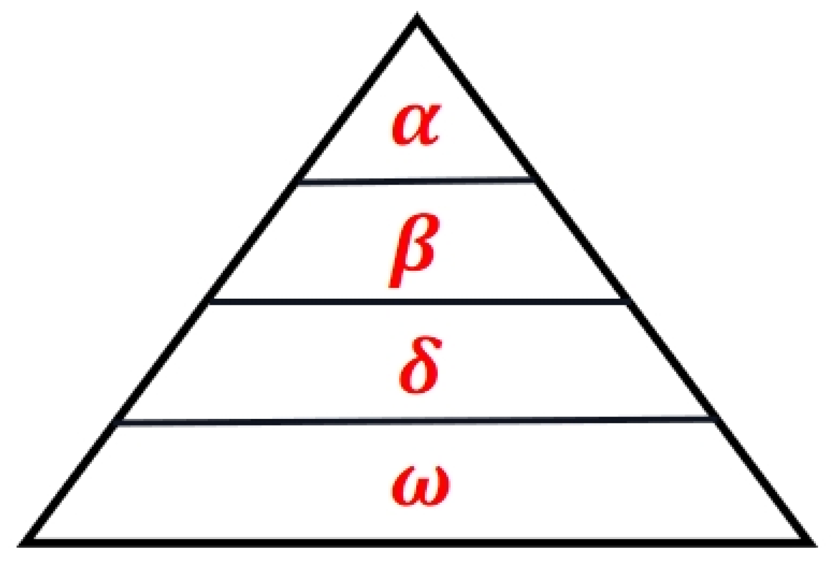
The position vector X in the grey wolf optimizer will consist of N individuals in the population of dimension d. Each individual represents a “grey wolf”, which has a social hierarchy, including “ α ” (the best individual), “ β ” (the second-best individual), “ δ ” (the third-best individual), and “ ω ” (the other individuals). The hierarchy is shown in Figure 1.
(1)
Encircling prey.
X ( t + 1 ) = X p ( t ) A · D
D = C · X p ( t ) X ( t )
where X p ( t ) is the current generation prey position, X ( t ) is the current generation grey wolf individual position, A and C are vector coefficients with formulas A = 2 a r 1 a and C = 2 r 2 , r 1 and r 2 are random numbers between the intervals [0,1], and a is the convergence factor, which decreases linearly from 2 to 0 as the number of iterations increases, i.e.,
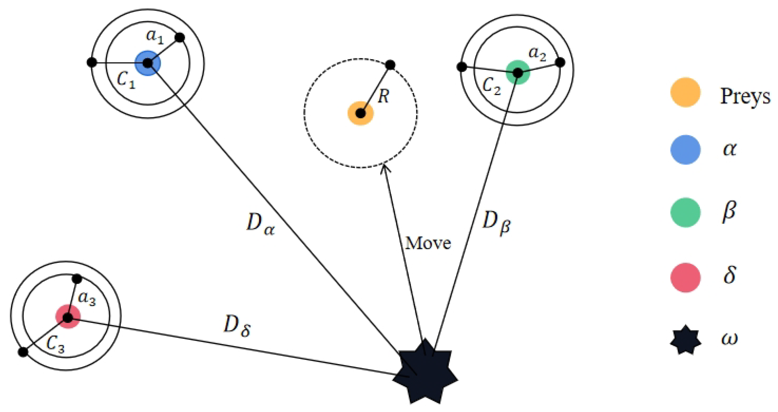
a = 2 2 t T max
(2)
Hunting. The positions of the other grey wolves in group X are jointly determined based on the positions of α , β , and δ :
X 1 ( t ) = X α ( t ) A 1 · D α , D α = C 1 · X α ( t ) X ( t )
X 2 ( t ) = X β ( t ) A 2 · D β , D β = C 2 · X β ( t ) X ( t )
X 3 ( t ) = X δ ( t ) A 3 · D δ , D δ = C 3 · X δ ( t ) X ( t )
X ( t + 1 ) = X 1 ( t ) + X 2 ( t ) + X 3 ( t ) / 3
where A 1 , A 2 , and A 3 are defined the same as A and C 1 , C 2 and C 3 are defined the same as C. The way of updating the wolf position is shown in the following Figure 2.

3.3. Follower Update Formulation Based on GWO and Escape Energy

In highly complex multimodal problems, the PFA may fall into local optimal solutions; this is because the PFA is mainly based on competition and selection among individuals, and may miss the global optimal solution in some cases. GWO excels in global search, leveraging population behavior and alignment mechanisms to effectively explore the search space and identify either the global optimal solution or a near-optimal one. In light of these strengths, this paper integrates the PFA with the GWO algorithm to enhance the overall performance of PFA.
To strike a balance between global and local search, and to further improve the search efficiency and optimization performance of the algorithm, the paper introduces the concept of escape energy (E) from the Harris Hawks optimization (HHO) [33]. Equation (19) captures this concept and is presented as follows:
E = 2 E 0 1 t T max
Here, E 0 represents a randomly generated number within the range of [−1,1]. The escape energy (E) plays a crucial role in determining the algorithm’s performance, influencing factors such as search speed, search quality, and convergence. When the escape energy E is greater than or equal to 1, it encourages individuals to engage in global exploration more frequently. This is particularly beneficial when the entire search space has not been thoroughly explored, aiding the algorithm in swiftly identifying potential globally optimal solutions during the initial iterations. Conversely, when the escape energy E is less than or equal to 1, individuals tend to prioritize local searches. They concentrate on delving deeper into regions near the currently identified superior solutions, facilitating the algorithm in optimizing those candidate solutions with a more detailed approach.
The follower update Equation (23) for the PFA, combining the GWO and the escape energy (E), is as follows:
x 1 t = x α t E · A 1 D α , D α = C 1 · x α t x t
x 2 t = x β t E · A 2 · D β , D β = C 2 · x β t x t
x 3 t = x δ t E · A 3 · D δ , D δ = C 3 · x δ t x t
x t + 1 = x 1 t + x 2 t + x 3 t / 3

3.4. Dimension-by-Dimension Mutation

The t-distribution [34,35], also known as the student distribution, has the following probability density (Equation (24)):
p ( x ) = Γ m + 1 2 m π Γ m 2 1 + x 2 2 m + 1 2
where Γ m + 1 2 = 0 + x m + 1 2 1 e x d x 
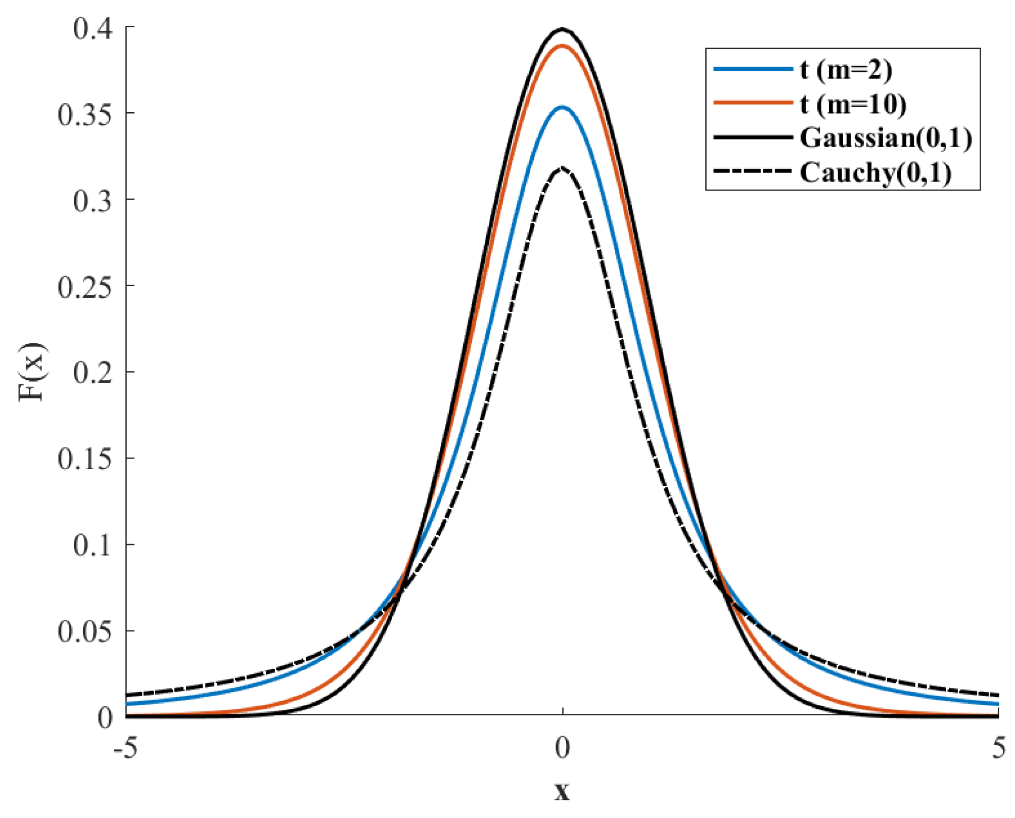
is the Euler integral of type II. The t-distribution curve shape is related to the value of the degrees of freedom parameter m. When the parameter m = 1, the t-distribution is in the form of a Cauchy distribution, denoted as t(m = 1) = C(0,1). As the parameter “m” increases, the t-distribution gradually approaches the standard normal distribution. When the parameter “m” tends to infinity, the t-distribution gradually converges to the standard normal distribution N(0,1). Figure 3 shows the distribution of the t-distribution, Cauchy distribution, and normal distribution with parameter changes for different degrees of freedom.
The output result of the mutation operation has uncertainty, and if the dimension-by-dimension mutation operation is performed on each individual in the population, it will inevitably lead to an increase in computational complexity and may reduce the search efficiency of the algorithm. Therefore, in this section, only the optimal individual in the current population is subjected to the dimension-by-dimension mutation operation, and the dimension-by-dimension mutation formula is as follows:
x n e w b e s t d = x b e s t d + x b e s t d × t i t e r
where t ( i t e r ) is the t-distribution of the PFA’s iteration count for the degree of freedom parameter, and x n e w b e s t d is the new solution following mutation. At the beginning of the iteration, i t e r is smaller, representing a smaller degree of the freedom parameter; the model is close to the Cauchy distribution, t ( i t e r ) has a significant role in the perturbation of the individual x b e s t d , which effectively enhances the algorithm’s ability to search globally, and helps to prevent the individual from falling into the local aggregation phenomenon. As the iteration of the algorithm proceeds, the increase in the degrees of freedom parameter causes the t distribution to gradually converge to a Gaussian distribution, which results in a gradual weakening of the perturbation of the distribution operator on the individual x b e s t d . This evolution is particularly evident in the later stages of the algorithm (where i t e r is larger), which in turn provides the algorithm with a higher degree of local exploitation and convergence accuracy.
Since the optimal individual position after mutation cannot be guaranteed to be better than the original position, an optimization-preserving strategy, i.e., greedy strategy, is added after the dimension-by-dimension mutation position perturbation. By comparing the fitness value of the mutated optimal individual with the original optimal individual, the individual with the best fitness value is selected as the global optimal solution for the current generation, then the mutated individual replaces the original individual, and the judgment formula is as follows:
x n e w b e s t d = x b e s t d f x b e s t d < f x n e w b e s t d x n e w b e s t d f x b e s t d f x n e w b e s t d

3.5. IPFA Steps

The IPFA algorithm’s specific steps and Algorithm 2 are as follows, based on the enhancements in this section:
Step 1: The initialized algorithm parameters, including population size (N), upper and lower boundaries ( u b and l b ) of the search range, and the maximum iterations ( T max );
Step 2: The population is initialized using the elite opposition-based learning strategy outlined in Equation (10);
Step 3: Computing the fitness values of each individual in the population based on a fitness function. Sort the individuals based on the fitness value and select the individual with the smallest fitness value as the pathfinder;
Step 4: Pathfinder phase. Update the pathfinder position according to Equation (2);
Step 5: Follower stage. Update the follower position according to Equation (23);
Step 6: Mutation stage. The fitness values of all individuals are computed and ranked, and then the individual with the optimal fitness value is picked for dimension-by-dimension mutation based on Equation (25);
Step 7: Determine whether to update the optimal individual according to the greedy strategy Equation (26);
Step 8: The population’s individual fitness levels are updated, and the person with the lowest value is selected to be the new pathfinder;
Step 9: If the termination condition for iterations is met, output the optimal individual position x b e s t t along with its corresponding fitness value. Otherwise, repeat Steps 4 through 9 until the iteration termination is satisfied.  
Algorithm 2 Pseudo-code of IPFA.
  1:
Initialize IPFA parameters
  2:
Initialize population using EOBL by using Equations (9) and (10)
  3:
When the elite opposition solution crosses the boundary utilizing Equation (11) update
  4:
Compute the initial value of population fitness
  5:
Individuals with the smallest fitness values were used as pathfinders
  6:
while t < maximum iterations do
  7:
   Update pathfinder the position using Equation (2) and check the bound
  8:
   if new pathfinder is better than old then
  9:
     Update pathfinder
10:
   end if
11:
   for i = 2 to maximum iterations do
12:
     Using Equation (19) to calculate the value of the escape factor E
13:
     Individual population fitness values were ranked to determine α , β , and δ wolf
14:
     Update follower the position using Equations (20)–(23) and check the bound
15:
   end for
16:
   Compute new fitness of the population
17:
   Find the best fitness
18:
   Dimension-by-dimension mutation of new best member using Equation (25)
19:
   if new best fitness > old best fitness then
20:
     Get a new best member using Equation (26)
21:
   else
22:
     Get a new best member using Equation (26)
23:
   end if
24:
   Compute new fitness of members
25:
   Find the best fitness
26:
   if best fitness < fitness of pathfinder then
27:
      pathfinder = best member
28:
      fitness = best fitness
29:
   end if
30:
    t = t + 1
31:
end while

3.6. Time Complexity Analysis

The total temporal complexity of the PFA is known to be O ( d + f ( d ) ) , assuming a population size of N, spatial dimensions of d, and a maximum iteration count of T max . In this scenario, f ( x ) represents the fitness function. The time complexity of the IPFA is now analyzed.
For the IPFA, in the initialization population stage, assuming the time for initializing algorithm parameters is t 1 , and the time for sorting all individuals based on fitness values and selecting the pathfinder is t 2 , the time complexity of the initialization population stage can be expressed as follows:
T 1 = O ( t 1 + N × f ( d ) + t 2 ) + O ( N × d ) = O ( d + f ( d ) )
Here, the time complexity for initializing the individuals in the population through elite opposition-based learning is O ( N × d ) , and the time for calculating the fitness value for each individual is f ( d ) .
As the iteration progresses, during the pathfinder phase, the IPFA updates the pathfinder position like the standard PFA, without incurring additional time. Consequently, the time complexity of the pathfinder phase remains consistent with that of the standard PFA, as follows:
T 2 = O ( d )
During the follower phase, the time required for computing the coefficient vectors A and C is denoted as t 3 . Additionally, the time for calculating the distances between α , β , and δ wolves for each individual in the population is represented by t 4 . The computation of X 1 ( t ) , X 2 ( t ) , and X 3 ( t ) consumes time t 5 , while the calculation of X ( t + 1 ) requires time t 6 . The processing time for the boundaries of the follower’s dimensions is denoted as t 7 , and the time for computing E is t 8 . Collectively, these components contribute to the time complexity of the follower phase:
T 3 = O ( ( N 1 ) × ( t 3 + 3 ( t 4 + t 5 ) + t 6 + d × t 7 + f ( d ) + t 8 ) ) = O ( d + f ( d ) )
During the mutation phase, the following time complexities are measured: t 9 is the time of sorting the population of individuals to find the optimal individual; t 10 is the time of the optimal individual performing dimension-by-dimension mutation; f ( d ) is the time of computing the fitness value of the optimal individual; t 11 is the time of determining whether the new optimal individual replaces the old optimal individual by using the greedy strategy; t 12 is the time of retaining the position of the optimal individual; and t 13 is the time of processing the boundaries of the optimal individual in each dimension, so the time complexity of the mutation phase is as follows:
T 4 = O ( 1 × d × ( t 10 + t 11 + t 13 ) + t 9 + t 12 + 1 × f ( d ) ) = O ( d + f ( d ) )
To put it briefly, the IPFA’s total temporal complexity is T = T 1 + T max ( T 2 + T 3 + T 4 ) = O ( d + f ( d ) ) . As a result, the IPFA’s time complexity and execution efficiency are comparable to those of the regular PFA.

4. Experimental Simulation and Analysis of Results

4.1. Experimental Design

To assess the performance of the proposed IPFA in this study, IPFA is compared with particle swarm optimization (PSO) [10], differential evolution (DE) [11], whale optimization algorithm (WOA) [12], seagull optimization algorithm (SOA) [36], sine cosine algorithm (SCA) [14], grey wolf optimizer (GWO) [30], chimp optimization algorithm (ChOA) [37], and the standard PFA [15] on 45 benchmark test functions (function information as shown in Table 1). The functions f 1 f 7 are unimodal (UN) functions, f 8 f 12 are multimodal (MN) functions, f 13 f 16 are fixed-dimension multimodal (FM) functions, and F1–F29 are benchmark test functions from CEC2017. In CEC2017, F1–F9 involve functions with rotation and translation tests, F10–F19 are composite functions designed to assess the algorithm’s capability in handling high-dimensional problems, and F20–F29 are hybrid functions designed to evaluate the algorithm’s performance under various complex scenarios. To ensure the fairness of the evaluation, each algorithm underwent 30 independent runs to minimize the possible effects of random samples. While maintaining uniformity, all algorithms shared a set of parameter settings, such as a population size of 30 and a maximum iteration of 1000. For the fairness of the experiment, all algorithms were subjected to optimization testing on a computer equipped with an Intel(R) Core(TM) i5—11260H CPU @ 2.60 GHz, running Windows 10, with 16 GB of memory and a 64-bit operating system. The optimization experiments were conducted using MATLAB R2021a software. Table 2 provides the parameter settings for each algorithm.

4.2. Comparative Analysis of Optimization Performance

In this section, a comprehensive comparison is conducted between IPFA and nine other evolutionary algorithms, with summarized results presented in Table 3. Three key metrics are analyzed for each algorithm: mean, standard deviation (S.D), and Best. The “Mean” represents the average obtained by summing the results of 30 independent runs of a specific algorithm and dividing by the number of runs. Also, the algorithms are ranked according to their average values, with the rankings starting from 1, representing the best performing algorithm, followed by a rank of 2, and so on; if there are multiple algorithms with equal performance, they are ranked the same, while the rankings of the other algorithms are computed in the usual order. The sum of the algorithm rankings on the test functions and the overall rankings are shown in the last two rows. The better an algorithm performs on each test function, the smaller the value of the sum of the rankings. Thus, the best algorithm has a composite ranking of 1, followed closely by algorithms with a ranking of 2, and so on.
Regarding the single-peak functions, f 1 , f 2 , f 6 , and f 7 , the IPFA obtains a performance of Rank 1, in terms of the mean, S.D., and best, but regarding the functions, f 4 , f 5 , and f 8 , the IPFA is only ranked 2nd, 5th, and 3rd, which is less than ideal for finding the optimal results. Overall, the convergence performance of IPFA on single-peaked functions is slightly better than the other eight algorithms.
The IPFA secures the top ranking on multi-peak functions f 11 and f 12 . However, its performance is less impressive on other multi-peak and fixed-dimensional multi-peak functions, where it holds the 6th, 2nd, 4th, and 3rd positions for functions f 10 , f 13 , and f 14 , respectively. It is important to remember that for these three functions, the ‘best’ is ideal.
In the evaluation of the CEC2017 functions F1-F23, the IPFA consistently secures the 1st rank across all rotation and displacement functions F1, F2, F3, F4, and F6. This remarkable performance indicates its exceptional capability to rotate the problem and effectively adapt to the translation of the search space. Moreover, the algorithm demonstrates resilience in overcoming geometric changes within the search space, underscoring its robust adaptability. The IPFA algorithm is ranked 1 for all high-dimensional composite functions except for the function F18. This observation suggests that the incorporation of the escape energy from the Harris Hawks optimization in the algorithm achieves a harmonious balance between a global and local search. This allows for rapid convergence to the global optimal solution, preventing entrapment in local optima. Moreover, it underscores the algorithm’s proficiency in handling high-dimensional functions. The IPFA achieves the 1st rank on mixed functions F25 and F27. These mixed functions exhibit highly complex shapes with pronounced nonlinearity, lack of smoothness, and irregular characteristics. The utilization of t-distribution-based multi-elite individuals for dimension-wise mutations in the algorithm proves beneficial for escaping the current position and converging toward the local minimum of the functions. This imparts significant adaptability to the algorithm, enabling it to overcome the challenges posed by the intricate nature of these functions. While the algorithm’s performance is suboptimal on the remaining eight functions, it notably outperforms other algorithms with the smallest best values on functions F20, F22, F26, F28, and F29. This underscores the algorithm’s superior optimization capability in comparison to the considered alternatives.
The IPFA secures the top position across all 45 function species in the search results, showcasing its exceptional global search and local exploration capabilities. The algorithm exhibits robustness and adaptability, further underscoring its prowess.
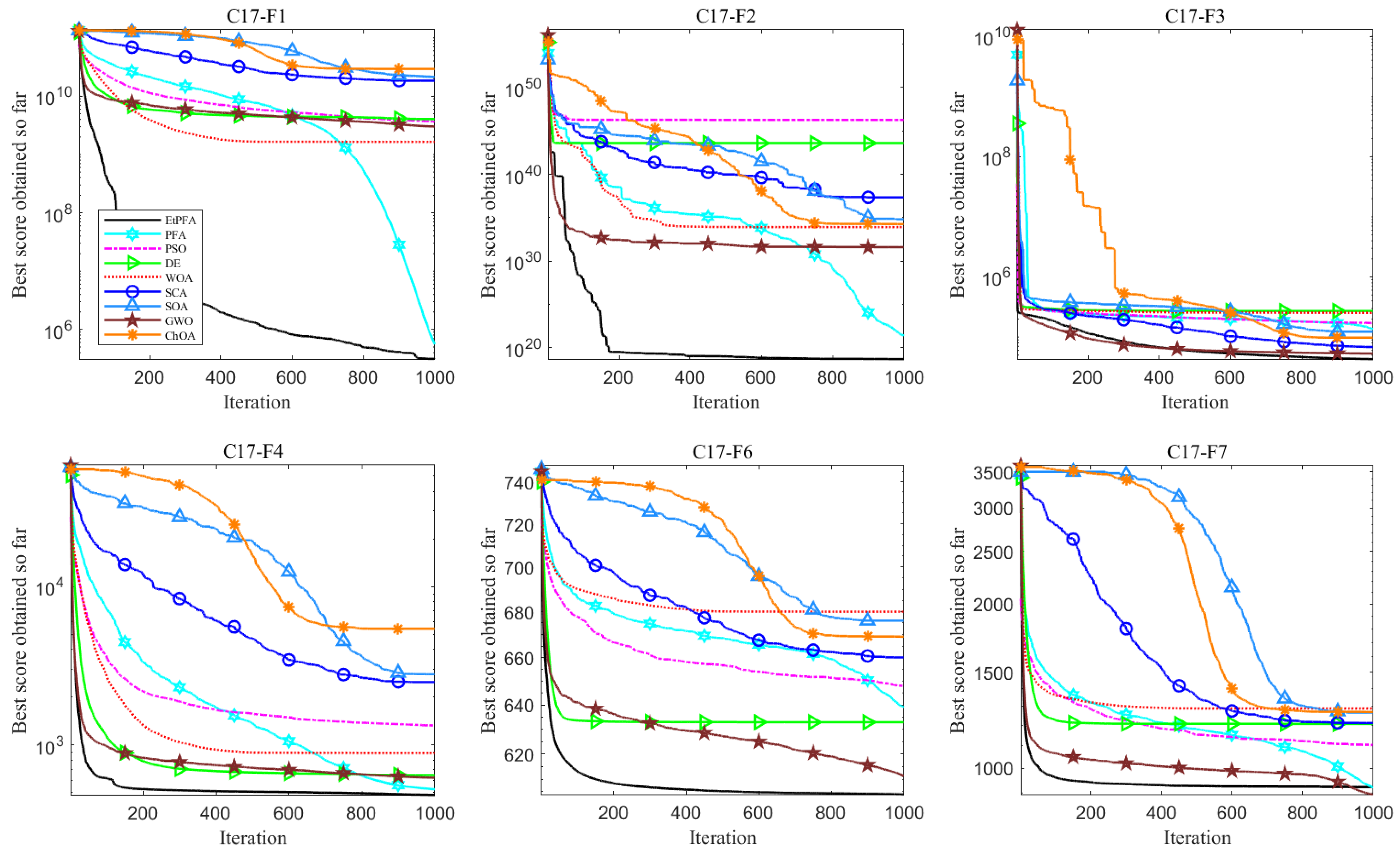
The convergence curves shown in Figure 4 and Figure 5 indicate that IPFA outperforms the other eight algorithms in terms of global convergence and overall optimized search accuracy. In addition, the boxplots in Figure 6 and Figure 7 illustrate the performance of these algorithms when dealing with test functions. Regarding unimodal functions f 1 f 7 , the IPFA only falls into local optima for functions f 3 , f 4 , and f 5 , demonstrating a notable advantage in the remaining functions. It rapidly converges toward the global optimum. Regarding multimodal functions f 8 f 12 , the IPFA notably lacks the high convergence accuracy observed in the WOA for functions f 8 f 10 and experiences local optima. However, it is evident that the IPFA exhibits a faster early-stage convergence, indicating that elite opposition-based learning provides superior initial solutions. These solutions are closer to the global optimum than randomly initialized solutions. Despite all algorithms encountering local optima in functions f 11 and f 12 , the IPFA significantly outperforms others in terms of convergence accuracy and speed. For fixed-dimensional multi-peaked functions f 13 f 16 , it can be seen that the PFA algorithm solves such functions more generally. This superiority arises from the characteristic nature of fixed-dimensional multi-peaked functions, which typically encompass numerous locally optimal solutions spaced relatively far apart. The dimension-by-dimension variation strategy employed by the IPFA concentrates solutions near certain local optima, hindering efficient escape and resulting in the algorithm being trapped in local convergence without the ability to explore global optimal solutions. In the realm of CEC2017 functions, the collaboration between the pathfinders and followers in the PFA has consistently exhibited superior optimization accuracy compared to other algorithms. Notably, for functions F7, F20, and F22, the PFA and GWO demonstrate continuous optimization efforts. However, the improved pathfinder algorithm (IPFA) outperforms all other algorithms on the remaining functions. This underscores the algorithm’s exceptional global search capability, enabling it to swiftly and efficiently navigate the problem’s search space and converge rapidly toward potential global optimal solutions.

4.3. Wilcoxon Rank Sum Test

One nonparametric hypothesis testing technique is the Wilcoxon signed-rank sum test (WRST) [38]. Because it refrains from making particular assumptions about the data distribution, it is very appropriate for a variety of intricate comparative data analyses. The Wilcoxon rank sum test (WRST) is a valuable tool for evaluating the convergence performance of multiple algorithms when comparing their performances. The outcomes of the nonparametric tests conducted through WRST are presented in Table 4 and Table 5.
Eight distinct algorithms were employed in this analysis, each subjected to a comparative evaluation against the IPFA algorithm. In each experiment, the discrepancies in observations across the algorithms were quantified and ranked, based on their absolute magnitudes, and assigned corresponding ranks. Subsequently, the algorithms were classified, based on the positive and negative scenarios of the rank, with ’+’ indicating a positive rank sum and ’-’ indicating a negative rank sum. The p-value was then used to determine if there was a significant difference between the two algorithms. If the p-value exceeds 0.05, it indicates that there is no statistically significant difference between the two algorithms. Simultaneously, the concept of a “winner” was introduced to delineate the algorithm’s performance relative to others in diverse situations.
Specifically, the magnitudes of positive and negative rank sums were compared when the p-value was less than 0.05. If the positive rank sum is less than the negative rank sum, it means that an algorithm shows an advantage in convergence performance compared to other algorithms at a statistical significance level of 5%, marking it as ’+’; on the contrary, if the positive rank sum is greater than the negative rank sum, it means that the algorithm shows a weaker performance at the significance level, marking it as ’-’; the p-value is marked with a ’=’ if it is larger than 0.05, which means that at the 5% significance level, there is no significant difference between the two algorithms.
In this way, the validity of the proposed IPFA algorithm is verified. Therefore, in this section, nonparametric tests are performed on the means in Table 3 using the Wilcoxon signed-rank sum test, the results of which are presented in Table 4 and Table 5, to authoritatively assess the convergence performance of the compared algorithms.
Table 4 and Table 5 demonstrate that in 27 of the 45 benchmark functions, the IPFA performs better than the PFA, there is no significant difference in 9 benchmark functions, and there are also 9 benchmark functions that are inferior to the PFA, and in general, the IPFA performs slightly better than the PFA, which indicates that the algorithm’s improvement has an effect; compared with the PSO, the performance of the IPFA is inferior to that of PSO except for the functions f 14 , f 15 , and f 16 , and the performance of the IPFA outperforms that of PSO for the rest of the 42 functions. Compared with the DE, except for 10 functions where the performance of the two algorithms is comparable, the DE is inferior to the IPFA in the remaining 35 functions; compared with the SCA, the IPFA outperforms the SCA in 45 functions. Compared to the GWO, IPFA has only slightly better performance; the IPFA has a significant advantage over the WOA, SOA, and ChOA in most of the functions. In conclusion, it is demonstrated that IPFA outperforms other intelligent optimization algorithms in terms of total performance.

4.4. Research on Engineering Design Problems of IPFA

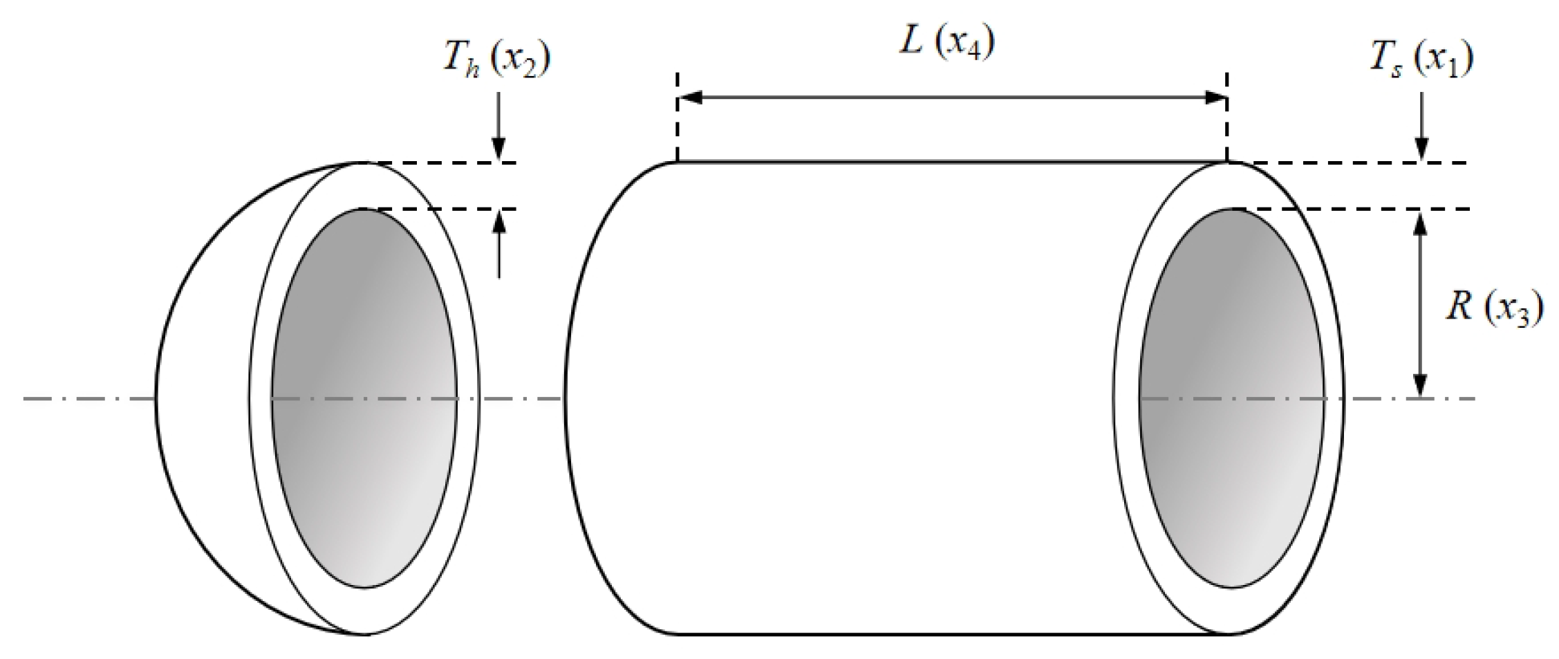
4.4.1. Pressure Vessel Design Problem

Reducing the total cost is the aim of the pressure vessel design challenge [39]. Four decision variables make up this model: the thickness of the shell T s ( 0 x 1 99 ) , the thickness of the head T h ( 0 x 2 99 ) , the inner radius R ( 0 x 3 200 ) , and the length of the cylindrical section without taking the head L s ( 10 x 4 200 ) , in addition to four constraints. The model’s schematic structure is displayed in Figure 8:
The mathematical model of the pressure vessel design problem is as follows:
min f X = 0.6224 x 1 x 2 x 3 + 1.7781 x 2 x 3 2 + 3.1661 x 1 2 x 4 + 19.84 x 1 2 x 3 s . t . g 1 ( X ) = x 1 + 0.0193 x 2 0 g 2 ( X ) = x 2 + 0.00954 x 3 0 g 3 X = π x 3 2 x 4 4 π x 3 3 3 + 1296000 0 g 4 ( X ) = x 4 240 0
To optimize this problem, the IPFA is initialized with 30 individuals, executed for 30 independent runs, and iterated for 1000 cycles. The final optimization outcome is f ( X ) = 5948.3597 with X = [0.9383 0.0628 54.6570 184.6838]. The results obtained by the proposed IPFA in solving this problem are compared with eight other optimization algorithms, including those reported in the literature. The experimental results are comprehensively presented in Table 6 and Table 7. Upon analyzing the tables, it is evident that the IPFA in this study exhibits superior optimization performance compared to the other six meta-heuristic algorithms. It not only incurs lower design costs but also boasts the smallest S.D. among all the algorithms. Furthermore, the mean and worst rank second only to PFA, underscoring the efficacy of IPFA in optimizing the pressure vessel design problem.

4.4.2. Tension Spring Design Problem

The tension spring design problem [43] has the objective of minimizing or maximizing the performance metrics of a tension spring under given constraints. This model has three decision variables: coil diameter d ( 0.05 x 1 2 ) , average coil diameter D ( 0.25 x 2 1.3 ) , and the number of active coils N ( 2 x 3 15 ) , as well as four constraints, and its structure is schematically shown in Figure 9:
The mathematical model of the tension spring design problem is as follows:
min f X = x 3 + 2 x 2 x 1 2 s . t . g 1 ( X ) = 1 x 2 3 x 3 71785 0 g 2 X = 4 x 2 2 x 1 x 2 12566 x 2 x 1 2 x 4 + 1 5108 x 1 2 1 0 g 3 ( X ) = 1 140.45 x 1 x 2 2 x 3 0 g 4 X = x 1 + x 2 1.5 1 0
The algorithm settings remain consistent with those employed in the pressure vessel design experiments. The results of each algorithm running independently for 30 iterations are tabulated in Table 8 and Table 9. Based on the provided tables, the mean, worst, and S.D. of the IPFA are comparatively average in comparison to other optimization algorithms. Although there is room for improvement in its performance, the IPFA and GWO optimums are minimized at the same time, which is excellent compared to the other seven meta-heuristic algorithms, demonstrating the lowest design cost with f ( X ) = 0.012699, X = [0.0504 0.3978 11.2764].

5. Conclusions

In this study, we propose an improved pathfinding algorithm (IPFA) to address the problems of slow convergence and low optimization accuracy of standard pathfinding algorithms. Firstly, we introduce an elite opposition-based learning learning mechanism that incorporates learned exemplar individuals at the beginning of the algorithm. This improvement aims to increase the diversity and quality of the entire population, thus improving the global optimality performance and increasing the convergence accuracy. By selectively integrating individuals with exceptional performance into the initial population, the algorithm is better equipped to explore a diverse solution space and mitigate premature convergence to local optima.
Secondly, integrating the escape energy into the prey-hunting phase of the grey wolf optimizer, while substituting the follower phase in the pathfinder algorithm, serves to enhance the algorithm’s diversity and elevate both the search efficiency and optimization performance. The incorporation of escape energy enables a subset of individuals to opt for escape during the search process, facilitating a more extensive exploration of the search space. This strategic approach helps prevent the algorithm from converging to a local optimal solution, thereby enhancing global search capabilities and fortifying the algorithm’s overall robustness.
In conclusion, the dimension-by-dimension mutation method is employed to perturb the location of the optimal individual, facilitating a swift escape from local optimal solutions and promoting movement toward alternative regions. By implementing tiny random perturbations on every dimension of the ideal individual, this method successfully breaks apart the local structure of the existing solution. As a result, this directs the search procedure in a novel and maybe more advantageous route, improving the algorithm’s overall search performance.
Incorporating these mechanisms into the pathfinder algorithm considers global optimization, diversity maintenance, escape mechanisms, and perturbation strategies. This comprehensive enhancement aims to improve the robustness and performance of the algorithm. Such depth in algorithmic improvement is typically well-suited to address the distinct characteristics of various problems, consequently enhancing the algorithm’s applicability.
Simultaneously, eight representative meta-heuristic algorithms were chosen for performance comparison, confirming the exceptional performance of the IPFA through function optimization experiments and an index evaluation system. The IPFA was successfully employed to address two engineering design problems, demonstrating stable and effective optimization outcomes that fully validate the algorithm’s robust applicability. In future research endeavors, the aim will be to explore the integration of the IPFA with the field of deep learning, applying the optimization model to data prediction and analysis problems.

Author Contributions

Conceptualization, B.W. and X.M.; methodology, X.M.; software, B.W.; data curation, W.Y. and Y.C.; writing—original draft preparation, X.M.; visualization, B.W., W.Y. and Y.C.; funding acquisition, B.W. and X.M. All authors have read and agreed to the published version of the manuscript.

Funding

This project was funded by the National Natural Science Foundation of China (grant no. 12271036), the Scientific Research Project of Mudanjiang Normal University (grant no. GP2020003), and the School-level Projects of Mudanjiang Normal University (grant no. kjcx2023-125mdjnu, kjcx2023-126mdjnu).

Data Availability Statement

Data are contained within the article.

Conflicts of Interest

The authors declare no conflicts of interest.

References

  1. Huo, X.; Zhang, F.; Shao, K.; Tan, J.Q. Improved Meta-heuristic Optimization Algorithm and Its Application in Image Segmentation. J. Softw. 2021, 32, 3452–3467. [Google Scholar]
  2. Rajamoorthy, R.; Arunachalam, G.; Kasinathan, P.; Devendiran, R.; Ahmadi, P.; Pandiyan, S.; Muthusamy, S.; Panchal, H.; Kazem, H.A.; Sharma, P. A novel intelligent transport system charging scheduling for electric vehicles using Grey Wolf Optimizer and Sail Fish Optimization algorithms. Energy Sources Part A Recover. Util. Environ. Eff. 2022, 44, 3555–3575. [Google Scholar] [CrossRef]
  3. He, Y.; Venkatesh, B.; Guan, L. Optimal scheduling for charging and discharging of electric vehicles. IEEE Trans. Smart Grid 2012, 3, 1095–1105. [Google Scholar] [CrossRef]
  4. Cai, Y.; Du, P. Path planning of unmanned ground vehicle based on balanced whale optimization algorithm. Control. Decis. 2021, 36, 2647–2655. [Google Scholar]
  5. Guerrero-Ibáñez, J.; Zeadally, S.; Contreras-Castillo, J. Sensor technologies for intelligent transportation systems. Sensors 2018, 18, 1212. [Google Scholar] [CrossRef]
  6. Xia, H.; Chen, L.; Wang, D.; Lu, X. Improved Denclue outlier detection algorithm with differential privacy and attribute fuzzy priority relation ordering. IEEE Access 2023, 11, 90283–90297. [Google Scholar] [CrossRef]
  7. Xia, H.Z.; Chen, L.M.; Qi, F.; Mao, X.D.; Sun, L.Q.; Xue, F.Y. DP-Denclue: An outlier detection algorithm with differential privacy preservation. In Proceedings of the 2022 IEEE 24th IEEE International Conference on High Performance Computing and Communications (HPCC), Chengdu, China, 18–21 December 2022; pp. 2264–2269. [Google Scholar]
  8. Hsu, Y.P.; Modiano, E.; Duan, L. Age of information: Design and analysis of optimal scheduling algorithms. In Proceedings of the 2017 IEEE International Symposium on Information Theory (ISIT), Aachen, Germany, 25–30 June 2017; pp. 561–565. [Google Scholar]
  9. Zhang, H.Y.; Lin, W.m.; Chen, A.X. Path planning for the mobile robot: A review. Symmetry 2018, 10, 450. [Google Scholar] [CrossRef]
  10. Shi, Y. Particle swarm optimization. IEEE Connect. 2004, 2, 8–13. [Google Scholar]
  11. Draa, A.; Chettah, K.; Talbi, H. A compound sinusoidal differential evolution algorithm for continuous optimization. Swarm Evol. Comput. 2019, 50, 100450. [Google Scholar] [CrossRef]
  12. Mirjalili, S.; Lewis, A. The whale optimization algorithm. Adv. Eng. Softw. 2016, 95, 51–67. [Google Scholar] [CrossRef]
  13. Mirjalili, S.; Mirjalili, S.M.; Hatamlou, A. Multi-verse optimizer: A nature-inspired algorithm for global optimization. Neural Comput. Appl. 2016, 27, 495–513. [Google Scholar] [CrossRef]
  14. Mirjalili, S. SCA: A sine cosine algorithm for solving optimization problems. Knowl.-Based Syst. 2016, 96, 120–133. [Google Scholar] [CrossRef]
  15. Yapici, H.; Cetinkaya, N. A new meta-heuristic optimizer: Pathfinder algorithm. Appl. Soft Comput. 2019, 78, 545–568. [Google Scholar] [CrossRef]
  16. Priyadarshani, S.; Subhashini, K.; Satapathy, J. Pathfinder algorithm optimized fractional order tilt-integral-derivative (FOTID) controller for automatic generation control of multi-source power system. Microsyst. Technol. 2021, 27, 23–35. [Google Scholar] [CrossRef]
  17. Janamala, V. A new meta-heuristic pathfinder algorithm for solving optimal allocation of solar photovoltaic system in multi-lateral distribution system for improving resilience. SN Appl. Sci. 2021, 3, 118. [Google Scholar] [CrossRef] [PubMed]
  18. Gouda, E.A.; Kotb, M.F.; El-Fergany, A.A. Investigating dynamic performances of fuel cells using pathfinder algorithm. Energy Convers. Manag. 2021, 237, 114099. [Google Scholar] [CrossRef]
  19. Yuan, Z.; Li, H.; Yousefi, N. Optimal hydrogen consumption of fuel cell-based locomotive using speed trajectory optimization by Improved Pathfinder algorithm. J. Clean. Prod. 2021, 278, 123430. [Google Scholar] [CrossRef]
  20. Tang, C.; Zhou, Y.; Luo, Q.; Tang, Z. An enhanced pathfinder algorithm for engineering optimization problems. Eng. Comput. 2021, 38, 1481–1503. [Google Scholar] [CrossRef]
  21. Tang, C.; Zhou, Y.; Tang, Z.; Luo, Q. Teaching-learning-based pathfinder algorithm for function and engineering optimization problems. Appl. Intell. 2021, 51, 5040–5066. [Google Scholar] [CrossRef]
  22. Hu, R.; Dong, Y.; Qian, B. Pathfinder algorithm for green pipeline scheduling with limited buffers. J. Syst. Simul. 2021, 33, 1384. [Google Scholar]
  23. Lu, M. Improvement and Application of Grey Wolf Optimization Algorithm. Master’s Thesis, Guangxi Minzun University, Nanning, China, 2021. [Google Scholar]
  24. Sun, Z.Z. Improved Pathfinder Algorithm and Its Application. Master’s Thesis, University of Science and Technology Liaoning, Anshan, China, 2021. [Google Scholar]
  25. Mahdavi, S.; Rahnamayan, S.; Deb, K. Opposition based learning: A literature review. Swarm Evol. Comput. 2018, 39, 1–23. [Google Scholar] [CrossRef]
  26. Tizhoosh, H.R. Opposition-based learning: A new scheme for machine intelligence. In Proceedings of the International Conference on Computational Intelligence for Modelling, Control and Automation and International Conference on Intelligent Agents, Web Technologies and Internet Commerce (CIMCA-IAWTIC’06), Vienna, Austria, 28–30 November 2005; Volume 1, pp. 695–701. [Google Scholar]
  27. Yildiz, B.S.; Pholdee, N.; Bureerat, S.; Yildiz, A.R.; Sait, S.M. Enhanced grasshopper optimization algorithm using elite opposition-based learning for solving real-world engineering problems. Eng. Comput. 2022, 38, 4207–4219. [Google Scholar] [CrossRef]
  28. Yuxin, G.; Sheng, L.; Wenxin, G.; Lei, Z. Elite Opposition-Based Learning Golden-Sine Harris Hawks Optimization. J. Comput. Eng. Appl. 2022, 58. [Google Scholar] [CrossRef]
  29. Xie, C.W.; Xu, L.; Zhao, H.R.; Xia, X.W.; Wei, B. Multi-objective fireworks optimization algorithm using elite opposition-based learning. Acta Electonica Sin. 2016, 44, 1180. [Google Scholar]
  30. Mirjalili, S.; Mirjalili, S.M.; Lewis, A. Grey wolf optimizer. Adv. Eng. Softw. 2014, 69, 46–61. [Google Scholar] [CrossRef]
  31. Zhang, X.; Lin, Q.; Mao, W.; Liu, S.; Dou, Z.; Liu, G. Hybrid Particle Swarm and Grey Wolf Optimizer and its application to clustering optimization. Appl. Soft Comput. 2021, 101, 107061. [Google Scholar] [CrossRef]
  32. Ou, Y.; Zhou, K.; Yin, P.; Liu, X. Improved grey wolf optimizer algorithm based on dual convergence factor strategy. J. Comput. Appl. 2023, 43, 2679. [Google Scholar]
  33. Kamboj, V.K.; Nandi, A.; Bhadoria, A.; Sehgal, S. An intensify Harris Hawks optimizer for numerical and engineering optimization problems. Appl. Soft Comput. 2020, 89, 106018. [Google Scholar] [CrossRef]
  34. Lange, K.L.; Little, R.J.; Taylor, J.M. Robust statistical modeling using the t distribution. J. Am. Stat. Assoc. 1989, 84, 881–896. [Google Scholar] [CrossRef]
  35. Jones, M.C.; Faddy, M. A skew extension of the t-distribution, with applications. J. R. Stat. Soc. Ser. Stat. Methodol. 2003, 65, 159–174. [Google Scholar] [CrossRef]
  36. Dhiman, G.; Kumar, V. Seagull optimization algorithm: Theory and its applications for large-scale industrial engineering problems. Knowl.-Based Syst. 2019, 165, 169–196. [Google Scholar] [CrossRef]
  37. Khishe, M.; Mosavi, M.R. Chimp optimization algorithm. Expert Syst. Appl. 2020, 149, 113338. [Google Scholar] [CrossRef]
  38. Wilcoxon, F. Individual comparisons by ranking methods. In Breakthroughs in Statistics: Methodology and Distribution; Springer: Berlin/Heidelberg, Germany, 1992; pp. 196–202. [Google Scholar]
  39. Moss, D.R. Pressure Vessel Design Manual; Elsevier: Amsterdam, The Netherlands, 2004. [Google Scholar]
  40. Abualigah, L.; Shehab, M.; Diabat, A.; Abraham, A. Selection scheme sensitivity for a hybrid Salp Swarm Algorithm: Analysis and applications. Eng. Comput. 2022, 38, 1149–1175. [Google Scholar] [CrossRef]
  41. Cheng, Z.; Song, H.; Zheng, D.; Zhou, M.; Sun, K. Hybrid firefly algorithm with a new mechanism of gender distinguishing for global optimization. Expert Syst. Appl. 2023, 224, 120027. [Google Scholar] [CrossRef]
  42. Montemurro, M.; Vincenti, A.; Vannucci, P. The automatic dynamic penalisation method (ADP) for handling constraints with genetic algorithms. Comput. Methods Appl. Mech. Eng. 2013, 256, 70–87. [Google Scholar] [CrossRef]
  43. Arora, J.S. Introduction to Optimum Design; Elsevier: Amsterdam, The Netherlands, 2004. [Google Scholar]
  44. Kaveh, A.; Bakhshpoori, T. Water evaporation optimization: A novel physically inspired optimization algorithm. Comput. Struct. 2016, 167, 69–85. [Google Scholar] [CrossRef]
  45. Feng, L.; Li, S.; Feng, S. Preparation and characterization of silicone rubber with high modulus via tension spring-type crosslinking. RSC Adv. 2017, 7, 13130–13137. [Google Scholar] [CrossRef]
  46. Kaveh, A.; Talatahari, S. A novel heuristic optimization method: Charged system search. Acta Mech. 2010, 213, 267–289. [Google Scholar] [CrossRef]
Figure 1. Grey wolf pyramid levels.
Symmetry 16 00324 g001
Figure 2. Schematic diagram of grey wolf location update.
Symmetry 16 00324 g002
Figure 3. Gaussian, t-distribution, and Cauchy distribution density functions.
Symmetry 16 00324 g003
Figure 4. Convergence curves of functions f 1 f 16 .
Symmetry 16 00324 g004aSymmetry 16 00324 g004b
Figure 5. CEC2017 functions: convergence curves (parts).
Symmetry 16 00324 g005aSymmetry 16 00324 g005b
Figure 6. Boxplot of functions f 1 f 16 .
Symmetry 16 00324 g006
Figure 7. Boxplot of CEC2017 functions (parts).
Symmetry 16 00324 g007
Figure 8. Pressure vessel design model.
Symmetry 16 00324 g008
Figure 9. Tension spring design model.
Symmetry 16 00324 g009
Table 1. Benchmark functions.
FunctionsFunction NameDimRange f min
f 1 Sphere100[−100, 100]0
f 2 Schwefel’s problem 2.22100[−10, 10]0
f 3 Schwefel’s problem 1.2100[−100, 100]0
f 4 Schwefel’s problem 2.21100[−100, 100]0
f 5 Rosenbrock100[−30, 30]0
f 6 Step100[−100, 100]0
f 7 Noise100[−1.28, 1.28]0
f 8 Rastrigin100[−5.12, 5.12]0
f 9 Ackley100[−32, 32]0
f 10 Griewank100[−600, 600]0
f 11 Generalized Penalized function 1100[−50, 50]0
f 12 Generalized Penalized function 2100[−50, 50]0
f 13 Hartman 26[0, 1]−3.32
f 14 Shekel 14[0, 10]−10.1532
f 15 Shekel 24[0, 10]−10.4028
f 16 Shekel 34[0, 10]−10.5363
CEC2017 Test Functions
F1Shifted and Rotated Bent Cigar Function30[−100, 100]100
F2Shifted and Rotated Zakharov Function30[−100, 100]200
F3Shifted and Rotated Rosenbrock Function30[−100, 100]300
F4Shifted and Rotated Rastrigin’s Function30[−100, 100]400
F5Shifted and Rotated Expanded Schaffer F6 Function30[−100, 100]500
F6Shifted and Rotated Lunacek Bi_ Rastrigin Function30[−100, 100]600
F7Shifted and Rotated Non-Continuous Rastrigin Function30[−100, 100]700
F8Shifted and Rotated Levy Function30[−100, 100]800
F9Shifted and Rotated Schwefel Function30[−100, 100]900
F10Hybrid Function 1 (N = 3)30[−100, 100]1000
F11Hybrid Function 2 (N = 3)30[−100, 100]1100
F12Hybrid Function 3 (N = 3)30[−100, 100]1200
F13Hybrid Function 4 (N = 4)30[−100, 100]1300
F14Hybrid Function 5 (N = 4)30[−100, 100]1400
F15Hybrid Function 6 (N = 4)30[−100, 100]1500
F16Hybrid Function 6 (N = 5)30[−100, 100]1600
F17Hybrid Function 6 (N = 5)30[−100, 100]1700
F18Hybrid Function 6 (N = 5)30[−100, 100]1800
F19Hybrid Function 6 (N = 6)30[−100, 100]1900
F20Composition Function 1 (N = 3)30[−100, 100]2000
F21Composition Function 2 (N = 3)30[−100, 100]2100
F22Composition Function 3 (N = 3)30[−100, 100]2200
F23Composition Function 4 (N = 3)30[−100, 100]2300
F24Composition Function 5 (N = 3)30[−100, 100]2400
F25Composition Function 6 (N = 3)30[−100, 100]2500
F26Composition Function 7 (N = 3)30[−100, 100]2600
F27Composition Function 8 (N = 3)30[−100, 100]2700
F28Composition Function 9 (N = 3)30[−100, 100]2800
F29Composition Function 10 (N = 3)30[−100, 100]2900
Table 2. Experimental parameters of each algorithm.
AlgorithmsYearsParameters
IPFAPresents = 0.5
PFA2019-
PSO1998w = 0.9, c 1 = c 2 = 2
WOA2016 a max = 2, a min = 0
DE1995F = 0.85, P C r = 0.8
SOA2019 f c = 2, u = v = 1
SCA2016a = 2
ChOA2020m = c h a o s (3, 1, 1)
GWO2014 a = 2 2 t T max
Table 3. Comparison of benchmarking function optimization results.
FunItemIPFAPFAPSODEWOASCASOAGWOChOA
f 1 Mean 1.1018 × 10 310 2.0180 × 10 02 7.5848 × 10 + 01 6.2796 × 10 + 02 6.0887 × 10 151 7.1948 × 10 02 2.1570 × 10 11 1.9133 × 10 58 4.0208 × 10 18
S.D 0.0000 × 10 + 00 1.7936 × 10 02 4.4935 × 10 + 01 1.6167 × 10 + 03 3.2862 × 10 150 1.9089 × 10 01 5.6886 × 10 11 8.6091 × 10 58 1.0360 × 10 17
Best 0.0000 × 10 + 00 2.2859 × 10 03 5.4413 × 10 + 00 8.4376 × 10 01 5.8209 × 10 167 4.3022 × 10 06 1.6932 × 10 16 4.9392 × 10 61 2.6633 × 10 28
Rank168927534
f 2 Mean 1.1775 × 10 174 4.8973 × 10 01 1.1154 × 10 + 01 1.1288 × 10 + 01 2.0410 × 10 102 2.1208 × 10 05 1.2090 × 10 11 1.1068 × 10 34 1.4656 × 10 12
S.D 0.0000 × 10 + 00 3.9074 × 10 01 8.9362 × 10 + 00 1.3686 × 10 + 01 9.4371 × 10 102 4.4957 × 10 05 2.2189 × 10 11 1.1958 × 10 34 2.6385 × 10 12
Best 2.8139 × 10 188 5.5184 × 10 02 2.9679 × 10 + 00 2.8200 × 10 03 6.7965 × 10 115 4.0508 × 10 08 6.6393 × 10 13 6.9846 × 10 36 1.1245 × 10 15
Rank178926534
f 3 Mean 4.6998 × 10 + 02 1.0129 × 10 + 03 6.4943 × 10 + 03 1.9042 × 10 + 04 2.1360 × 10 + 04 3.5608 × 10 + 03 5.2716 × 10 + 02 2.4137 × 10 14 3.6267 × 10 02
S.D 4.6667 × 10 + 02 1.1733 × 10 + 03 5.1031 × 10 + 03 1.1123 × 10 + 04 9.6159 × 10 + 03 3.0275 × 10 + 03 1.3073 × 10 + 03 1.2595 × 10 13 7.5598 × 10 02
Best 2.0910 × 10 + 01 1.5814 × 10 + 01 3.5172 × 10 + 02 2.5963 × 10 + 03 5.6903 × 10 + 03 3.3794 × 10 + 02 9.9885 × 10 02 2.0600 × 10 19 9.7881 × 10 06
Rank357896412
f 4 Mean 7.3219 × 10 08 3.1580 × 10 + 00 4.0909 × 10 + 00 6.9796 × 10 + 01 4.6767 × 10 + 01 2.1025 × 10 + 01 1.8440 × 10 01 2.2443 × 10 14 2.2341 × 10 03
S.D 6.7708 × 10 08 1.4103 × 10 + 00 1.6530 × 10 + 00 9.6208 × 10 + 00 2.8508 × 10 + 01 9.4814 × 10 + 00 3.0242 × 10 01 2.3272 × 10 145 1.0264 × 10 02
Best 2.2086 × 10 09 5.9025 × 10 01 1.6779 × 10 + 00 5.0193 × 10 + 01 2.7382 × 10 04 8.9974 × 10 + 00 1.0988 × 10 02 5.6557 × 10 16 4.6896 × 10 07
Rank256987413
f 5 Mean 5.3791 × 10 + 01 5.6585 × 10 + 01 1.7017 × 10 + 03 5.7367 × 10 + 06 2.7392 × 10 + 01 5.0864 × 10 + 02 2.8595 × 10 + 01 2.6796 × 10 + 01 2.8837 × 10 + 01
S.D 4.3437 × 10 + 01 3.6634 × 10 + 01 2.1718 × 10 + 03 8.6591 × 10 + 06 6.6294 × 10 01 1.5720 × 10 + 03 3.2503 × 10 01 6.7781 × 10 01 1.9958 × 10 01
Best 1.7417 × 10 + 01 1.9217 × 10 + 01 7.8145 × 10 + 01 1.1467 × 10 + 03 2.6727 × 10 + 01 2.7940 × 10 + 01 2.8118 × 10 + 01 2.5252 × 10 + 01 2.8057 × 10 + 01
Rank569928314
f 6 Mean 2.6384 × 10 05 2.0423 × 10 02 7.3081 × 10 + 01 6.3670 × 10 + 02 8.9580 × 10 02 4.4493 × 10 + 00 1.1827 × 10 + 00 6.6292 × 10 01 3.2993 × 10 + 00
S.D 1.1385 × 10 05 2.3094 × 10 02 4.3693 × 10 + 01 1.2204 × 10 + 03 1.0282 × 10 01 3.8119 × 10 01 2.9815 × 10 01 3.0481 × 10 01 3.6342 × 10 01
Best 8.1525 × 10 06 7.3713 × 10 04 1.3054 × 10 + 01 4.5141 × 10 02 9.0726 × 10 03 3.4658 × 10 + 00 6.4310 × 10 01 2.4684 × 10 01 2.4030 × 10 + 00
Rank138947526
f 7 Mean 2.4457 × 10 04 1.4076 × 10 02 1.6285 × 10 01 7.8505 × 10 + 00 1.3892 × 10 03 3.7151 × 10 02 3.4790 × 10 02 7.8588 × 10 04 8.1494 × 10 04
S.D 2.6070 × 10 04 8.8628 × 10 03 4.8588 × 10 01 7.4746 × 10 + 00 1.3605 × 10 03 5.3369 × 10 02 2.1584 × 10 02 4.0907 × 10 04 1.1463 × 10 03
Best 1.4739 × 10 05 1.6585 × 10 03 1.5829 × 10 02 3.1174 × 10 01 3.7655 × 10 05 2.0600 × 10 03 1.2667 × 10 03 1.3397 × 10 04 5.7108 × 10 05
Rank158947623
f 8 Mean 2.8422 × 10 14 1.0318 × 10 + 01 1.6881 × 10 + 02 1.4179 × 10 + 02 0.0000 × 10 + 00 1.2877 × 10 + 01 4.4798 × 10 11 7.5791 × 10 15 3.0970 × 10 + 00
S.D 3.8784 × 10 14 1.5015 × 10 + 01 3.3957 × 10 + 01 4.7013 × 10 + 01 0.0000 × 10 + 00 1.8824 × 10 + 01 1.1829 × 10 10 1.9653 × 10 14 6.2301 × 10 + 00
Best 0.0000 × 10 + 00 1.2513 × 10 03 9.8430 × 10 + 01 6.0802 × 10 + 01 0.0000 × 10 + 00 1.7284 × 10 06 5.6843 × 10 14 0.0000 × 10 + 00 0.0000 × 10 + 00
Rank369817425
f 9 Mean 5.0981 × 10 14 2.9496 × 10 + 00 3.6389 × 10 + 00 1.9908 × 10 + 01 3.8488 × 10 15 1.2234 × 10 + 01 4.3185 × 10 07 1.5810 × 10 14 1.9962 × 10 + 01
S.D 9.6667 × 10 15 1.0718 × 10 + 00 7.3778 × 10 01 3.3649 × 10 01 2.3012 × 10 15 9.7507 × 10 + 00 7.2421 × 10 07 2.3603 × 10 15 1.2530 × 10 03
Best 3.2863 × 10 14 1.3302 × 10 02 2.2662 × 10 + 00 1.8128 × 10 + 01 8.8818 × 10 16 1.2084 × 10 04 1.3093 × 10 08 1.1546 × 10 14 1.9959 × 10 + 01
Rank356817429
f 10 Mean 4.4107 × 10 02 7.5884 × 10 02 1.5283 × 10 + 00 5.4793 × 10 + 00 0.0000 × 10 + 00 2.1841 × 10 01 4.6609 × 10 03 3.6932 × 10 03 7.0510 × 10 03
S.D 5.0855 × 10 02 4.9250 × 10 02 3.2849 × 10 01 6.8166 × 10 + 00 0.0000 × 10 + 00 2.4852 × 10 01 2.5529 × 10 02 8.4703 × 10 03 1.6606 × 10 02
Best 0.0000 × 10 + 00 1.3812 × 10 02 1.0446 × 10 + 00 5.3830 × 10 02 0.0000 × 10 + 00 5.7019 × 10 06 2.5979 × 10 14 0.0000 × 10 + 00 0.0000 × 10 + 00
Rank678915324
f 11 Mean 2.2248 × 10 03 8.6189 × 10 01 2.2523 × 10 + 00 3.0666 × 10 + 07 5.0271 × 10 03 2.4780 × 10 + 00 7.5739 × 10 02 3.6638 × 10 02 4.6837 × 10 01
S.D 1.2174 × 10 02 1.1806 × 10 + 00 1.3740 × 10 + 00 7.8781 × 10 + 07 4.8553 × 10 03 3.7241 × 10 + 00 3.7425 × 10 02 1.4697 × 10 02 2.3966 × 10 01
Best 2.2561 × 10 07 1.1358 × 10 04 5.3460 × 10 01 4.8681 × 10 + 02 8.0551 × 10 04 4.8240 × 10 01 2.7712 × 10 02 1.3180 × 10 02 2.0163 × 10 01
Rank167928435
f 12 Mean 8.1691 × 10 02 4.1812 × 10 01 7.5252 × 10 + 00 4.1546 × 10 + 07 2.1369 × 10 01 2.5411 × 10 + 01 2.7503 × 10 + 00 5.0768 × 10 01 2.8482 × 10 + 00
S.D 1.0356 × 10 01 3.2602 × 10 01 3.2403 × 10 + 00 5.1088 × 10 + 07 1.7601 × 10 01 1.0642 × 10 + 02 9.5287 × 10 02 1.7414 × 10 01 1.4988 × 10 01
Best 7.3265 × 10 06 3.0413 × 10 02 3.0930 × 10 + 00 9.1490 × 10 + 03 1.7585 × 10 02 2.1445 × 10 + 00 2.5406 × 10 + 00 1.9263 × 10 01 2.4480 × 10 + 00
Rank127938546
f 13 Mean 3.2665 × 10 + 00 3.2744 × 10 + 00 3.0301 × 10 + 00 3.1891 × 10 + 00 3.2173 × 10 + 00 2.9486 × 10 + 00 2.4973 × 10 + 00 3.2644 × 10 + 00 2.4371 × 10 + 00
S.D 7.6819 × 10 02 5.9241 × 10 02 3.3020 × 10 01 1.1387 × 10 01 1.0235 × 10 01 2.9583 × 10 01 6.3663 × 10 01 7.4374 × 10 02 4.9850 × 10 01
Best 3.3220 × 10 + 00 3.3220 × 10 + 00 3.3219 × 10 + 00 3.3220 × 10 + 00 3.3219 × 10 + 00 3.1661 × 10 + 00 3.0156 × 10 + 00 3.3220 × 10 + 00 3.0699 × 10 + 00
Rank216547839
f 14 Mean 8.5353 × 10 + 00 1.0153 × 10 + 01 9.3357 × 10 + 00 5.1037 × 10 + 00 8.4517 × 10 + 00 2.4910 × 10 + 00 7.3343 × 10 01 9.4791 × 10 + 00 2.8980 × 10 + 00
S.D 2.7552 × 10 + 00 6.4471 × 10 15 2.2166 × 10 + 00 3.0334 × 10 + 00 2.4427 × 10 + 00 2.0921 × 10 + 00 1.5860 × 10 01 1.7469 × 10 + 00 2.1059 × 10 + 00
Best 1.0152 × 10 + 01 1.0153 × 10 + 01 1.0153 × 10 + 01 1.0153 × 10 + 01 1.0153 × 10 + 01 6.2745 × 10 + 00 1.1276 × 10 + 00 1.0153 × 10 + 01 5.0469 × 10 + 00
Rank413657928
f 15 Mean 9.7286 × 10 + 00 1.0403 × 10 + 01 9.6957 × 10 + 00 5.8579 × 10 + 00 8.1441 × 10 + 00 3.7514 × 10 + 00 8.9447 × 10 01 1.0403 × 10 + 01 3.7733 × 10 + 00
S.D 2.0113 × 10 + 00 6.5972 × 10 16 1.8260 × 10 + 00 3.6030 × 10 + 00 3.1109 × 10 + 00 2.2774 × 10 + 00 3.3004 × 10 01 2.3476 × 10 04 1.9370 × 10 + 00
Best 1.0402 × 10 + 01 1.0403 × 10 + 01 1.0403 × 10 + 01 1.0403 × 10 + 01 1.0403 × 10 + 01 8.9582 × 10 + 00 2.2132 × 10 + 00 1.0403 × 10 + 01 5.0688 × 10 + 00
Rank213547816
f 16 Mean 8.1022 × 10 + 00 9.5146 × 10 + 00 1.0351 × 10 + 01 6.8025 × 10 + 00 9.1024 × 10 + 00 4.4693 × 10 + 00 9.6138 × 10 01 1.0266 × 10 + 01 4.0959 × 10 + 00
S.D 3.5173 × 10 + 00 2.6583 × 10 + 00 9.7766 × 10 01 3.7992 × 10 + 00 2.6919 × 10 + 00 1.9074 × 10 + 00 2.2087 × 10 01 1.4814 × 10 + 00 1.7673 × 10 + 00
Best 1.0533 × 10 + 01 1.0536 × 10 + 01 1.0536 × 10 + 01 1.0536 × 10 + 01 1.0536 × 10 + 01 9.0906 × 10 + 00 1.5282 × 10 + 00 1.0536 × 10 + 01 5.1066 × 10 + 00
Rank531647928
F1Mean 3.2031 × 10 + 05 3.8477 × 10 + 05 4.4096 × 10 + 09 2.5608 × 10 + 09 1.5124 × 10 + 09 1.9143 × 10 + 10 2.2417 × 10 + 10 3.0315 × 10 + 09 2.8477 × 10 + 10
S.D 1.7839 × 10 + 05 2.7042 × 10 + 05 4.5147 × 10 + 09 3.9989 × 10 + 09 8.0454 × 10 + 08 2.9889 × 10 + 09 3.6710 × 10 + 09 1.7244 × 10 + 09 5.7881 × 10 + 09
Best 1.0000 × 10 + 05 1.2654 × 10 + 05 9.4917 × 10 + 08 1.1604 × 10 + 05 5.8993 × 10 + 08 1.4205 × 10 + 10 1.5594 × 10 + 10 4.3512 × 10 + 08 1.7267 × 10 + 10
Rank126437859
F2Mean 3.2597 × 10 + 16 3.1168 × 10 + 20 7.7651 × 10 + 40 4.4781 × 10 + 38 4.0970 × 10 + 34 3.7841 × 10 + 37 5.5771 × 10 + 34 4.0208 × 10 + 31 6.2372 × 10 + 34
S.D 1.4430 × 10 + 17 1.6332 × 10 + 21 2.3723 × 10 + 41 2.3261 × 10 + 39 2.2182 × 10 + 35 1.1458 × 10 + 38 5.9430 × 10 + 34 1.8976 × 10 + 32 1.6308 × 10 + 35
Best 6.8586 × 10 + 08 1.1816 × 10 + 15 3.3609 × 10 + 26 1.9980 × 10 + 24 1.3264 × 10 + 25 1.0354 × 10 + 32 1.3585 × 10 + 31 9.4065 × 10 + 17 2.5089 × 10 + 28
Rank129847536
F3Mean 3.5133 × 10 + 04 1.1406 × 10 + 05 1.4559 × 10 + 05 2.8678 × 10 + 05 2.6799 × 10 + 05 7.2540 × 10 + 04 1.2867 × 10 + 05 5.3046 × 10 + 04 9.0166 × 10 + 04
S.D 7.7838 × 10 + 03 3.1471 × 10 + 04 6.7237 × 10 + 04 9.3639 × 10 + 04 6.5367 × 10 + 04 1.1034 × 10 + 04 2.5446 × 10 + 04 9.2375 × 10 + 03 1.1815 × 10 + 04
Best 2.1456 × 10 + 04 5.1345 × 10 + 04 4.8397 × 10 + 04 1.3216 × 10 + 05 1.6389 × 10 + 05 4.9470 × 10 + 04 9.1851 × 10 + 04 3.5006 × 10 + 04 6.2633 × 10 + 04
Rank156983724
F4Mean 4.8025 × 10 + 02 5.3420 × 10 + 02 1.2661 × 10 + 03 6.9072 × 10 + 02 8.3609 × 10 + 02 2.3814 × 10 + 03 3.0966 × 10 + 03 6.2332 × 10 + 02 6.6924 × 10 + 03
S.D 2.4508 × 10 + 01 3.6579 × 10 + 01 8.2219 × 10 + 02 2.4902 × 10 + 02 1.8324 × 10 + 02 6.2395 × 10 + 02 1.6125 × 10 + 03 7.6240 × 10 + 01 3.8537 × 10 + 03
Best 4.2153 × 10 + 02 4.7811 × 10 + 02 5.9131 × 10 + 02 4.7530 × 10 + 02 5.6490 × 10 + 02 1.5935 × 10 + 03 1.6294 × 10 + 03 5.1902 × 10 + 02 1.8798 × 10 + 03
Rank135457829
F5Mean 6.2748 × 10 + 02 6.7506 × 10 + 02 7.7137 × 10 + 02 7.0768 × 10 + 02 8.2436 × 10 + 02 8.1259 × 10 + 02 8.4089 × 10 + 02 6.1896 × 10 + 02 8.3368 × 10 + 02
S.D 2.8065 × 10 + 01 4.2444 × 10 + 01 4.0632 × 10 + 01 6.4519 × 10 + 01 5.0080 × 10 + 01 1.7890 × 10 + 01 2.3815 × 10 + 01 3.7013 × 10 + 01 3.4435 × 10 + 01
Best 5.7272 × 10 + 02 5.9728 × 10 + 02 6.9902 × 10 + 02 5.5651 × 10 + 02 7.2355 × 10 + 02 7.7859 × 10 + 02 7.9316 × 10 + 02 5.7676 × 10 + 02 7.5516 × 10 + 02
Rank235476918
F6Mean 6.0437 × 10 + 02 6.3732 × 10 + 02 6.4583 × 10 + 02 6.3622 × 10 + 02 6.7947 × 10 + 02 6.6093 × 10 + 02 6.7676 × 10 + 02 6.1108 × 10 + 02 6.7170 × 10 + 02
S.D 3.3460 × 10 + 00 9.4945 × 10 + 00 1.3812 × 10 + 01 1.4159 × 10 + 01 1.1513 × 10 + 01 8.1954 × 10 + 00 4.0893 × 10 + 00 3.8978 × 10 + 00 7.0330 × 10 + 00
Best 6.0044 × 10 + 02 6.1964 × 10 + 02 6.2539 × 10 + 02 6.1065 × 10 + 02 6.5740 × 10 + 02 6.3950 × 10 + 02 6.6739 × 10 + 02 6.0375 × 10 + 02 6.5509 × 10 + 02
Rank145396827
F7Mean 9.1901 × 10 + 02 9.2109 × 10 + 02 1.0923 × 10 + 03 1.2915 × 10 + 03 1.3030 × 10 + 03 1.2140 × 10 + 03 1.2523 × 10 + 03 8.9029 × 10 + 02 1.2618 × 10 + 03
S.D 5.5400 × 10 + 01 5.8953 × 10 + 01 5.5427 × 10 + 01 2.8304 × 10 + 02 1.0158 × 10 + 02 3.6266 × 10 + 01 4.0721 × 10 + 01 4.7196 × 10 + 01 4.4554 × 10 + 01
Best 8.2121 × 10 + 02 8.2913 × 10 + 02 9.8539 × 10 + 02 9.6088 × 10 + 02 1.0884 × 10 + 03 1.1396 × 10 + 03 1.1869 × 10 + 03 8.3976 × 10 + 02 1.1679 × 10 + 03
Rank234895617
F8Mean 9.1677 × 10 + 02 9.4171 × 10 + 02 1.0393 × 10 + 03 9.9407 × 10 + 02 1.0486 × 10 + 03 1.0787 × 10 + 03 1.0811 × 10 + 03 9.0647 × 10 + 02 1.0828 × 10 + 03
S.D 3.3583 × 10 + 01 3.6845 × 10 + 01 4.5076 × 10 + 01 6.3144 × 10 + 01 5.1836 × 10 + 01 2.2188 × 10 + 01 2.1102 × 10 + 01 2.5680 × 10 + 01 2.3501 × 10 + 01
Best 8.6992 × 10 + 02 8.7869 × 10 + 02 9.7723 × 10 + 02 8.8824 × 10 + 02 9.6004 × 10 + 02 1.0434 × 10 + 03 1.0307 × 10 + 03 8.6384 × 10 + 02 1.0258 × 10 + 03
Rank245367819
F9Mean 3.8547 × 10 + 03 3.0937 × 10 + 03 5.8847 × 10 + 03 8.6777 × 10 + 03 1.0007 × 10 + 04 7.7026 × 10 + 03 9.1212 × 10 + 03 2.4220 × 10 + 03 8.4320 × 10 + 03
S.D 1.2123 × 10 + 03 1.2522 × 10 + 03 2.6928 × 10 + 03 4.1457 × 10 + 03 2.9150 × 10 + 03 1.1743 × 10 + 03 1.1518 × 10 + 03 1.2459 × 10 + 03 1.5339 × 10 + 03
Best 1.2662 × 10 + 03 1.1054 × 10 + 03 2.9701 × 10 + 03 3.0616 × 10 + 03 5.1769 × 10 + 03 5.5565 × 10 + 03 6.8441 × 10 + 03 1.0207 × 10 + 03 5.6489 × 10 + 03
Rank324895716
F10Mean 4.3076 × 10 + 03 5.5265 × 10 + 03 7.2979 × 10 + 03 7.6795 × 10 + 03 7.0343 × 10 + 03 8.7115 × 10 + 03 7.5729 × 10 + 03 8.6346 × 10 + 03 8.6540 × 10 + 03
S.D 6.5432 × 10 + 02 8.6930 × 10 + 02 7.6825 × 10 + 02 1.1535 × 10 + 03 7.4749 × 10 + 02 4.0612 × 10 + 02 4.7822 × 10 + 02 2.6047 × 10 + 02 2.2182 × 10 + 02
Best 3.1236 × 10 + 03 3.9800 × 10 + 03 5.4293 × 10 + 03 5.0911 × 10 + 03 5.6275 × 10 + 03 7.6354 × 10 + 03 6.4401 × 10 + 03 7.5530 × 10 + 03 8.2531 × 10 + 03
Rank125749638
F11Mean 1.2018 × 10 + 03 1.4173 × 10 + 03 4.6497 × 10 + 03 4.9019 × 10 + 03 7.4108 × 10 + 03 3.2053 × 10 + 03 4.4522 × 10 + 03 2.1514 × 10 + 03 4.5684 × 10 + 03
S.D 2.7703 × 10 + 01 9.0032 × 10 + 01 7.4643 × 10 + 03 5.7398 × 10 + 03 2.5008 × 10 + 03 9.3077 × 10 + 02 8.4370 × 10 + 02 8.8683 × 10 + 02 1.1343 × 10 + 03
Best 1.1536 × 10 + 03 1.2730 × 10 + 03 1.5958 × 10 + 03 1.2967 × 10 + 03 2.5724 × 10 + 03 2.1251 × 10 + 03 2.5780 × 10 + 03 1.3184 × 10 + 03 2.7426 × 10 + 03
Rank127894536
F12Mean 8.2985 × 10 + 06 8.4177 × 10 + 06 6.1703 × 10 + 08 6.2965 × 10 + 07 2.3812 × 10 + 08 2.1908 × 10 + 09 2.2938 × 10 + 09 9.8263 × 10 + 07 6.8252 × 10 + 09
S.D 1.1901 × 10 + 07 7.0883 × 10 + 06 9.0651 × 10 + 08 1.7005 × 10 + 08 1.5908 × 10 + 08 5.3778 × 10 + 08 1.0459 × 10 + 09 8.3703 × 10 + 07 3.2651 × 10 + 09
Best 4.9157 × 10 + 05 5.7449 × 10 + 05 3.4099 × 10 + 07 4.1067 × 10 + 05 3.0842 × 10 + 07 1.0328 × 10 + 09 6.0040 × 10 + 08 5.0473 × 10 + 06 2.7086 × 10 + 09
Rank129356748
F13Mean 4.2649 × 10 + 04 1.3986 × 10 + 05 6.7844 × 10 + 08 6.5946 × 10 + 07 2.1645 × 10 + 06 8.0275 × 10 + 08 4.0367 × 10 + 08 2.6393 × 10 + 07 5.7390 × 10 + 09
S.D 2.3305 × 10 + 04 8.9848 × 10 + 04 1.4467 × 10 + 09 3.2724 × 10 + 08 1.6684 × 10 + 06 2.8392 × 10 + 08 7.6943 × 10 + 08 6.9637 × 10 + 07 4.7275 × 10 + 09
Best 4.5744 × 10 + 03 2.4576 × 10 + 04 7.7534 × 10 + 05 7.8561 × 10 + 03 4.0791 × 10 + 05 3.8632 × 10 + 08 2.7978 × 10 + 07 2.6701 × 10 + 04 1.2994 × 10 + 08
Rank127538649
F14Mean 8.2788 × 10 + 04 8.5509 × 10 + 04 9.7754 × 10 + 05 4.0456 × 10 + 05 1.9903 × 10 + 06 4.2828 × 10 + 05 4.4783 × 10 + 05 5.5038 × 10 + 05 1.2593 × 10 + 06
S.D 1.4833 × 10 + 05 6.3780 × 10 + 04 3.4757 × 10 + 06 7.1797 × 10 + 05 2.4778 × 10 + 06 3.0649 × 10 + 05 4.9449 × 10 + 05 7.6649 × 10 + 05 1.7075 × 10 + 06
Best 2.2287 × 10 + 03 3.3063 × 10 + 03 1.7826 × 10 + 04 4.7497 × 10 + 03 4.2143 × 10 + 04 3.9759 × 10 + 04 5.5357 × 10 + 04 3.0602 × 10 + 04 1.1296 × 10 + 05
Rank127394568
F15Mean 2.2402 × 10 + 04 5.8515 × 10 + 04 8.1276 × 10 + 05 3.1002 × 10 + 07 2.3077 × 10 + 06 5.0355 × 10 + 07 7.8371 × 10 + 06 2.4859 × 10 + 06 9.5456 × 10 + 07
S.D 2.3225 × 10 + 04 4.9457 × 10 + 04 7.6847 × 10 + 05 1.6475 × 10 + 08 3.9023 × 10 + 06 2.9236 × 10 + 07 1.3077 × 10 + 07 1.0367 × 10 + 07 4.0691 × 10 + 08
Best 2.7296 × 10 + 03 8.6259 × 10 + 03 7.3810 × 10 + 04 1.8291 × 10 + 03 5.2271 × 10 + 04 7.4482 × 10 + 06 2.5170 × 10 + 05 1.6488 × 10 + 04 1.8609 × 10 + 06
Rank123748659
F16Mean 2.7121 × 10 + 03 3.0447 × 10 + 03 3.6287 × 10 + 03 3.5558 × 10 + 03 4.1014 × 10 + 03 4.0332 × 10 + 03 3.8178 × 10 + 03 4.1852 × 10 + 03 4.1105 × 10 + 03
S.D 2.7593 × 10 + 02 4.0471 × 10 + 02 5.0065 × 10 + 02 5.6068 × 10 + 02 5.6221 × 10 + 02 2.3612 × 10 + 02 3.0471 × 10 + 02 3.5916 × 10 + 02 3.7665 × 10 + 02
Best 2.0122 × 10 + 03 2.3213 × 10 + 03 2.9486 × 10 + 03 1.9482 × 10 + 03 3.2065 × 10 + 03 3.5054 × 10 + 03 3.2284 × 10 + 03 3.6689 × 10 + 03 3.5176 × 10 + 03
Rank124376598
F17Mean 2.1407 × 10 + 03 2.4179 × 10 + 03 2.5769 × 10 + 03 2.5874 × 10 + 03 2.6818 × 10 + 03 2.6567 × 10 + 03 2.6308 × 10 + 03 2.0917 × 10 + 03 3.2590 × 10 + 03
S.D 1.9680 × 10 + 02 2.5815 × 10 + 02 3.4084 × 10 + 02 3.3583 × 10 + 02 2.6156 × 10 + 02 1.8352 × 10 + 02 1.6227 × 10 + 02 1.9005 × 10 + 02 1.3088 × 10 + 03
Best 1.7951 × 10 + 03 2.0814 × 10 + 03 1.9739 × 10 + 03 1.8476 × 10 + 03 2.1446 × 10 + 03 2.3263 × 10 + 03 2.3473 × 10 + 03 1.8437 × 10 + 03 2.4275 × 10 + 03
Rank234587619
F18Mean 1.0108 × 10 + 06 1.6471 × 10 + 06 2.1618 × 10 + 07 1.7515 × 10 + 07 1.0735 × 10 + 07 9.0368 × 10 + 06 1.5038 × 10 + 06 1.3408 × 10 + 06 3.7312 × 10 + 06
S.D 9.0803 × 10 + 05 2.3211 × 10 + 06 7.9669 × 10 + 07 3.3616 × 10 + 07 9.2493 × 10 + 06 4.3702 × 10 + 06 8.1194 × 10 + 05 1.6433 × 10 + 06 1.9271 × 10 + 06
Best 1.2574 × 10 + 05 7.6547 × 10 + 04 3.9099 × 10 + 05 1.9034 × 10 + 05 2.2865 × 10 + 05 3.8986 × 10 + 06 3.5949 × 10 + 05 1.4792 × 10 + 05 6.0237 × 10 + 05
Rank149876325
F19Mean 1.0245 × 10 + 04 2.8419 × 10 + 05 1.1608 × 10 + 07 2.5108 × 10 + 06 1.4933 × 10 + 07 7.2644 × 10 + 07 3.1410 × 10 + 07 8.0087 × 10 + 05 6.2082 × 10 + 08
S.D 9.6215 × 10 + 03 2.8579 × 10 + 05 3.9655 × 10 + 07 1.2544 × 10 + 07 1.6643 × 10 + 07 4.5453 × 10 + 07 4.4058 × 10 + 07 1.1964 × 10 + 06 8.2664 × 10 + 08
Best 2.1822 × 10 + 03 3.2526 × 10 + 04 1.0743 × 10 + 05 2.5511 × 10 + 03 1.5216 × 10 + 05 2.8965 × 10 + 06 1.7347 × 10 + 06 1.3678 × 10 + 04 2.4740 × 10 + 07
Rank125469738
F20Mean 2.5016 × 10 + 03 2.6103 × 10 + 03 2.7478 × 10 + 03 3.0946 × 10 + 03 2.9299 × 10 + 03 2.8502 × 10 + 03 2.7753 × 10 + 03 2.4158 × 10 + 03 3.1307 × 10 + 03
S.D 1.8747 × 10 + 02 1.8793 × 10 + 02 2.2633 × 10 + 02 3.3156 × 10 + 02 2.5956 × 10 + 02 1.3199 × 10 + 02 1.6163 × 10 + 02 1.0027 × 10 + 02 1.5944 × 10 + 02
Best 2.2101 × 10 + 03 2.2547 × 10 + 03 2.2403 × 10 + 03 2.5342 × 10 + 03 2.4882 × 10 + 03 2.4937 × 10 + 03 2.5064 × 10 + 03 2.2629 × 10 + 03 2.7606 × 10 + 03
Rank234876519
F21Mean 2.4544 × 10 + 03 2.4682 × 10 + 03 2.5575 × 10 + 03 2.4834 × 10 + 03 2.6184 × 10 + 03 2.5878 × 10 + 03 2.6097 × 10 + 03 2.4077 × 10 + 03 2.5975 × 10 + 03
S.D 4.2970 × 10 + 01 4.5204 × 10 + 01 4.3387 × 10 + 01 6.5060 × 10 + 01 7.6117 × 10 + 01 2.2646 × 10 + 01 2.4117 × 10 + 01 3.0143 × 10 + 01 3.4120 × 10 + 01
Best 2.3794 × 10 + 03 2.3771 × 10 + 03 2.4707 × 10 + 03 2.3980 × 10 + 03 2.5022 × 10 + 03 2.5443 × 10 + 03 2.5494 × 10 + 03 2.3563 × 10 + 03 2.4993 × 10 + 03
Rank235496817
F22Mean 5.4008 × 10 + 03 3.6862 × 10 + 03 6.5564 × 10 + 03 8.6375 × 10 + 03 7.5657 × 10 + 03 9.8280 × 10 + 03 6.0989 × 10 + 03 4.5680 × 10 + 03 9.9134 × 10 + 03
S.D 1.6378 × 10 + 03 2.1666 × 10 + 03 2.8172 × 10 + 03 1.9543 × 10 + 03 1.9040 × 10 + 03 1.2932 × 10 + 03 1.6862 × 10 + 03 1.7447 × 10 + 03 2.2289 × 10 + 02
Best 2.3042 × 10 + 03 2.3059 × 10 + 03 2.6614 × 10 + 03 2.8120 × 10 + 03 2.7455 × 10 + 03 4.4365 × 10 + 03 4.0314 × 10 + 03 2.3699 × 10 + 03 9.2662 × 10 + 03
Rank325768419
F23Mean 2.8632 × 10 + 03 2.8515 × 10 + 03 3.2755 × 10 + 03 2.8440 × 10 + 03 3.0942 × 10 + 03 3.0547 × 10 + 03 3.0277 × 10 + 03 2.7709 × 10 + 03 3.1096 × 10 + 03
S.D 6.4030 × 10 + 01 4.8214 × 10 + 01 2.1503 × 10 + 02 7.1286 × 10 + 01 9.4794 × 10 + 01 4.0942 × 10 + 01 2.4572 × 10 + 01 4.0442 × 10 + 01 4.9032 × 10 + 01
Best 2.7421 × 10 + 03 2.7367 × 10 + 03 2.9140 × 10 + 03 2.7323 × 10 + 03 2.9213 × 10 + 03 2.9592 × 10 + 03 2.9833 × 10 + 03 2.7343 × 10 + 03 3.0236 × 10 + 03
Rank439276518
F24Mean 3.1439 × 10 + 03 2.9964 × 10 + 03 3.6837 × 10 + 03 3.0314 × 10 + 03 3.2140 × 10 + 03 3.2203 × 10 + 03 3.2186 × 10 + 03 2.9305 × 10 + 03 3.3219 × 10 + 03
S.D 8.6642 × 10 + 01 5.2673 × 10 + 01 2.2246 × 10 + 02 6.9814 × 10 + 01 1.0941 × 10 + 02 3.1077 × 10 + 01 2.5481 × 10 + 01 4.9094 × 10 + 01 4.6278 × 10 + 01
Best 3.0059 × 10 + 03 2.9051 × 10 + 03 3.3540 × 10 + 03 2.9251 × 10 + 03 3.0350 × 10 + 03 3.1723 × 10 + 03 3.1726 × 10 + 03 2.8725 × 10 + 03 3.2491 × 10 + 03
Rank429357618
F25Mean 2.8906 × 10 + 03 2.9307 × 10 + 03 3.1579 × 10 + 03 3.0033 × 10 + 03 3.1069 × 10 + 03 3.3901 × 10 + 03 3.6917 × 10 + 03 3.0091 × 10 + 03 4.4745 × 10 + 03
S.D 1.1971 × 10 + 01 2.2101 × 10 + 01 9.4472 × 10 + 01 1.4912 × 10 + 02 5.4413 × 10 + 01 1.5695 × 10 + 02 3.0194 × 10 + 02 7.1573 × 10 + 01 5.4389 × 10 + 02
Best 2.8813 × 10 + 03 2.8886 × 10 + 03 3.0194 × 10 + 03 2.8926 × 10 + 03 3.0310 × 10 + 03 3.1806 × 10 + 03 3.3264 × 10 + 03 2.9357 × 10 + 03 3.4101 × 10 + 03
Rank126357849
F26Mean 5.5592 × 10 + 03 5.4684 × 10 + 03 7.2510 × 10 + 03 5.7929 × 10 + 03 8.4663 × 10 + 03 7.6331 × 10 + 03 6.8978 × 10 + 03 4.9280 × 10 + 03 7.2914 × 10 + 03
S.D 8.9380 × 10 + 02 8.1585 × 10 + 02 1.5604 × 10 + 03 6.8537 × 10 + 02 8.3105 × 10 + 02 3.8632 × 10 + 02 2.3730 × 10 + 02 4.6748 × 10 + 02 4.9225 × 10 + 02
Best 2.8133 × 10 + 03 3.1385 × 10 + 03 3.8296 × 10 + 03 4.5415 × 10 + 03 6.7174 × 10 + 03 6.9848 × 10 + 03 6.1900 × 10 + 03 4.1351 × 10 + 03 6.3202 × 10 + 03
Rank326498517
F27Mean 3.2000 × 10 + 03 3.3003 × 10 + 03 3.6542 × 10 + 03 3.2632 × 10 + 03 3.4134 × 10 + 03 3.5118 × 10 + 03 3.5036 × 10 + 03 3.2740 × 10 + 03 3.7410 × 10 + 03
S.D 3.5746 × 10 04 8.4381 × 10 + 01 3.3626 × 10 + 02 3.0128 × 10 + 01 1.2073 × 10 + 02 7.6528 × 10 + 01 4.8087 × 10 + 01 3.5391 × 10 + 01 1.5108 × 10 + 02
Best 3.2000 × 10 + 03 3.2330 × 10 + 03 3.2558 × 10 + 03 3.2174 × 10 + 03 3.2842 × 10 + 03 3.3841 × 10 + 03 3.4055 × 10 + 03 3.2164 × 10 + 03 3.4900 × 10 + 03
Rank138457629
F28Mean 3.2934 × 10 + 03 3.2887 × 10 + 03 3.9852 × 10 + 03 3.9408 × 10 + 03 3.5815 × 10 + 03 4.2227 × 10 + 03 3.9834 × 10 + 03 3.5191 × 10 + 03 4.9530 × 10 + 03
S.D 2.2046 × 10 + 01 3.6787 × 10 + 01 1.0041 × 10 + 03 6.7247 × 10 + 02 1.3088 × 10 + 02 2.3651 × 10 + 02 2.8420 × 10 + 02 1.8424 × 10 + 02 7.4931 × 10 + 02
Best 3.2119 × 10 + 03 3.2251 × 10 + 03 3.3372 × 10 + 03 3.2399 × 10 + 03 3.3711 × 10 + 03 3.8666 × 10 + 03 3.6869 × 10 + 03 3.3142 × 10 + 03 3.7515 × 10 + 03
Rank217548639
F29Mean 3.9505 × 10 + 03 4.3798 × 10 + 03 4.8424 × 10 + 03 4.4459 × 10 + 03 5.3745 × 10 + 03 5.0495 × 10 + 03 4.6276 × 10 + 03 3.8568 × 10 + 03 4.8108 × 10 + 03
S.D 2.4865 × 10 + 02 2.6757 × 10 + 02 7.2174 × 10 + 02 4.0600 × 10 + 02 3.9015 × 10 + 02 3.1166 × 10 + 02 1.6918 × 10 + 02 2.1939 × 10 + 02 2.7074 × 10 + 02
Best 3.4629 × 10 + 03 3.7985 × 10 + 03 3.9964 × 10 + 03 3.7717 × 10 + 03 4.6358 × 10 + 03 4.3992 × 10 + 03 4.1722 × 10 + 03 3.5280 × 10 + 03 4.3074 × 10 + 03
Rank237498516
Total Rank88142267281244302266108310
Final Rank136678529
Table 4. WRST comparison between IPFA and PFA, PSO, DE, and WOA.
FunIPFA vs. PFAIPFA vs. PSOIPFA vs. DEIPFA vs. WOA
p-ValueR+R−Winnerp-ValueR+R−Winnerp-ValueR+R−Winnerp-ValueR+R−Winner
f 1 2.3657 × 10 12 0465+ 2.3657 × 10 12 0465+ 2.3657 × 10 12 0465+ 2.3657 × 10 12 0465+
f 2 3.0199 × 10 11 0465+ 3.0199 × 10 11 0465+ 3.0199 × 10 11 0465+ 3.0199 × 10 11 0465+
f 3 7.6171 × 10 03 179286+ 2.1544 × 10 10 0465+ 3.0199 × 10 11 0465+ 3.0199 × 10 11 0465+
f 4 3.0199 × 10 11 0465+ 3.0199 × 10 11 0465+ 3.0199 × 10 11 0465+ 3.0199 × 10 11 0465+
f 5 4.5146 × 10 02 193272+ 8.1527 × 10 11 0465+ 3.0199 × 10 11 0465+ 5.2014 × 10 01 182283+
f 6 3.0199 × 10 11 0465+ 3.0199 × 10 11 0465+ 3.0199 × 10 11 0465+ 3.0199 × 10 11 0465+
f 7 3.0199 × 10 11 0465+ 3.0199 × 10 11 0465+ 3.0199 × 10 11 0465+ 1.6351 × 10 05 38427+
f 8 1.4900 × 10 11 0465+ 1.4900 × 10 11 0465+ 1.4900 × 10 11 0465+ 1.3780 × 10 04 2130+
f 9 2.5856 × 10 11 0465+ 2.5856 × 10 11 0465+ 2.5692 × 10 11 0465+ 1.3946 × 10 11 4650+
f 10 9.5922 × 10 03 187278+ 2.5206 × 10 11 0465+ 9.2212 × 10 11 0465+ 8.8658 × 10 07 2980+
f 11 1.2057 × 10 10 0465+ 3.0199 × 10 11 0465+ 3.0199 × 10 11 0465+ 5.5727 × 10 10 27438+
f 12 3.6459 × 10 08 65400+ 3.0199 × 10 11 0465+ 3.0199 × 10 11 0465+ 2.8389 × 10 04 136329+
f 13 8.8669 × 10 04 335130+ 1.0277 × 10 06 84381+ 1.8047 × 10 01 239226= 2.2539 × 10 04 141324+
f 14 1.4488 × 10 11 4650 9.8461 × 10 06 39273 3.7412 × 10 02 128337+ 5.5699 × 10 03 281184
f 15 4.0806 × 10 12 4650 1.6617 × 10 04 347118 9.6027 × 10 02 152313= 3.0418 × 10 01 236229=
f 16 1.2551 × 10 07 43134 3.5149 × 10 08 43431 3.2402 × 10 01 268197= 3.9881 × 10 04 335130
F1 6.1001 × 10 01 153312 3.0199 × 10 11 0465+ 7.3803 × 10 10 20445+ 3.0199 × 10 11 0465+
F2 2.1544 × 10 10 6459 3.0199 × 10 11 0465+ 3.0199 × 10 11 0465+ 3.0199 × 10 11 0465+
F3 3.0199 × 10 11 0465 4.0772 × 10 11 0465+ 3.0199 × 10 11 0465+ 3.0199 × 10 11 0465+
F4 7.1186 × 10 09 15450+ 3.0199 × 10 11 0465+ 1.1737 × 10 09 44421+ 3.0199 × 10 11 0465+
F5 8.2919 × 10 06 106359+ 3.0199 × 10 11 0465+ 1.8731 × 10 07 61404+ 3.0199 × 10 11 0465+
F6 3.0199 × 10 11 0465+ 3.0199 × 10 11 0465+ 4.5043 × 10 11 0465+ 3.0199 × 10 11 0465+
F7 9.9410 × 10 01 239226= 9.9186 × 10 11 0465+ 8.1527 × 10 11 0465+ 3.0199 × 10 11 0465+
F8 4.5530 × 10 01 200265= 7.3803 × 10 10 3462+ 2.3885 × 10 04 140325+ 1.1737 × 10 09 0465+
F9 2.4157 × 10 02 300165 1.1143 × 10 03 108357+ 1.1567 × 10 07 44421+ 8.1527 × 10 11 0465+
F10 5.5999 × 10 07 24441+ 4.0772 × 10 11 0465+ 5.4941 × 10 11 0465+ 4.5043 × 10 11 0465+
F11 3.0199 × 10 11 0465+ 3.0199 × 10 11 0465+ 3.0199 × 10 11 0465+ 3.0199 × 10 11 0465+
F12 1.2597 × 10 01 193272= 4.9752 × 10 11 0465+ 1.6238 × 10 01 203262= 4.5043 × 10 11 0465+
F13 1.0666 × 10 07 57408+ 3.0199 × 10 11 0465+ 1.1199 × 10 01 120345= 3.0199 × 10 11 0465+
F14 8.5338 × 10 01 259206= 3.6709 × 10 03 158307+ 3.1830 × 10 01 137328= 6.0104 × 10 08 57408+
F15 2.7726 × 10 05 63402+ 3.6897 × 10 11 0465+ 4.7335 × 10 01 205260= 4.0772 × 10 11 0465+
F16 1.2362 × 10 03 97368+ 1.3289 × 10 10 0465+ 5.9673 × 10 09 12453+ 3.0199 × 10 11 0465+
F17 4.9426 × 10 05 112353+ 1.2860 × 10 06 73392+ 7.5991 × 10 07 103362+ 2.2273 × 10 09 24441+
F18 4.3764 × 10 01 235230= 6.2828 × 10 06 65400+ 1.0277 × 10 06 46419+ 1.2541 × 10 07 94371+
F19 4.9752 × 10 11 0465+ 3.0199 × 10 11 0465+ 9.5207 × 10 04 127338+ 3.0199 × 10 11 0465+
F20 1.9883 × 10 02 91374+ 6.3560 × 10 05 86379+ 2.0338 × 10 09 6459+ 6.0104 × 10 08 69396+
F21 2.5805 × 10 01 212253= 8.8910 × 10 10 0465+ 1.5367 × 10 01 207258= 1.3289 × 10 10 23442+
F22 1.4945 × 10 01 301164= 6.0971 × 10 03 149316+ 1.0105 × 10 08 74391+ 1.1077 × 10 06 66399+
F23 8.4180 × 10 01 128337= 1.0937 × 10 10 0465+ 1.7613 × 10 01 330135= 1.7769 × 10 10 0465+
F24 4.9980 × 10 09 43629 3.0199 × 10 11 0465+ 2.6784 × 10 06 38382 1.4412 × 10 02 196269+
F25 1.8567 × 10 09 6459+ 3.0199 × 10 11 0465+ 5.5727 × 10 10 5460+ 3.0199 × 10 11 0465+
F26 8.5338 × 10 01 258207= 1.1937 × 10 06 81384+ 3.4029 × 10 01 202263= 4.5043 × 10 11 0465+
F27 3.0199 × 10 11 0465+ 3.0199 × 10 11 0465+ 3.0199 × 10 11 0465+ 3.0199 × 10 11 0465+
F28 2.3243 × 10 02 315150 3.0199 × 10 11 0465+ 4.6159 × 10 10 9456+ 3.0199 × 10 11 0465+
F29 2.0283 × 10 07 21444+ 1.5465 × 10 09 25440+ 8.1975 × 10 07 45420+ 3.0199 × 10 11 0465+
+/=/- 27/9/9 42/0/3 35/10/0 42/1/2
Table 5. WRST comparison between IPFA and SCA, SOA, GWO, and ChOA.
FunIPFA vs. SCAIPFA vs. SOAIPFA vs. GWOIPFA vs. ChOA
p-ValueR+R−Winnerp-ValueR+R−Winnerp-ValueR+R−Winnerp-ValueR+R−Winner
f 1 2.3657 × 10 12 0465+ 1.1738 × 10 03 0465+ 3.0199 × 10 11 0465+ 2.3657 × 10 12 0465+
f 2 3.0199 × 10 11 0465+ 3.0199 × 10 11 0465+ 3.0199 × 10 11 0465+ 3.0199 × 10 11 0465+
f 3 1.4110 × 10 09 26439+ 7.7272 × 10 02 323142 3.0199 × 10 11 4650 3.0199 × 10 11 4650
f 4 3.0199 × 10 11 0465+ 3.0199 × 10 11 0465+ 3.0199 × 10 11 4650 3.0199 × 10 11 0465+
f 5 1.7666 × 10 03 160305+ 3.0199 × 10 11 171294= 4.6427 × 10 01 253212= 7.7272 × 10 02 171294=
f 6 3.0199 × 10 11 0465+ 4.8218 × 10 11 0465+ 3.0199 × 10 11 0465+ 3.0199 × 10 11 0465+
f 7 3.0199 × 10 11 0465+ 2.5856 × 10 11 0465+ 8.4848 × 10 09 46419+ 2.8389 × 10 04 140325+
f 8 1.4900 × 10 11 0465+ 2.8186 × 10 01 0434+ 2.6733 × 10 01 8874= 6.9360 × 10 10 0425+
f 9 2.5856 × 10 11 0465+ 1.4643 × 10 10 0465+ 4.4427 × 10 12 4650 2.5856 × 10 11 0465+
f 10 3.2146 × 10 03 97368+ 3.0199 × 10 11 284181= 1.4809 × 10 07 35467 2.0266 × 10 02 29891=
f 11 3.0199 × 10 11 0465+ 3.0199 × 10 11 0465+ 3.0199 × 10 11 0465+ 3.0199 × 10 11 0465+
f 12 3.0199 × 10 11 0465+ 3.0199 × 10 11 0465+ 8.8910 × 10 10 0465+ 3.0199 × 10 11 0465+
f 13 8.1527 × 10 11 25440+ 3.0199 × 10 11 0465+ 1.9112 × 10 02 314151 3.0199 × 10 11 0465+
f 14 2.4386 × 10 09 27438+ 3.0199 × 10 11 0465+ 4.1127 × 10 07 40758 2.2273 × 10 09 28437+
f 15 2.2273 × 10 09 9456+ 3.0199 × 10 11 0465+ 3.0199 × 10 11 4650 1.6947 × 10 09 0465+
f 16 4.2175 × 10 04 69396+ 3.0199 × 10 11 0465+ 7.3803 × 10 10 43827 8.6634 × 10 05 57408+
F1 3.0199 × 10 11 0465+ 3.0199 × 10 11 0465+ 3.0199 × 10 11 0465+ 3.0199 × 10 11 0465+
F2 3.0199 × 10 11 0465+ 3.0199 × 10 11 0465+ 3.6897 × 10 11 0465+ 3.0199 × 10 11 0465+
F3 3.3384 × 10 11 0465+ 3.0199 × 10 11 0465+ 1.3703 × 10 03 87378+ 3.0199 × 10 11 0465+
F4 3.0199 × 10 11 0465+ 3.0199 × 10 11 0465+ 1.3289 × 10 10 6459+ 3.0199 × 10 11 0465+
F5 3.0199 × 10 11 0465+ 3.0199 × 10 11 0465+ 1.0763 × 10 02 341124 3.0199 × 10 11 0465+
F6 3.0199 × 10 11 0465+ 3.3384 × 10 11 0465+ 3.1967 × 10 09 27438+ 3.0199 × 10 11 0465+
F7 3.0199 × 10 11 0465+ 3.3384 × 10 11 0465+ 5.0842 × 10 03 337128 3.0199 × 10 11 0465+
F8 3.0199 × 10 11 0465+ 3.0199 × 10 11 0465+ 1.3853 × 10 06 39768 3.3384 × 10 11 0465+
F9 7.3891 × 10 11 0465+ 3.0199 × 10 11 0465+ 1.2362 × 10 03 340125 6.0658 × 10 11 0465+
F10 3.0199 × 10 11 0465+ 3.0199 × 10 11 0465+ 1.9579 × 10 01 146319= 3.0199 × 10 11 0465+
F11 3.0199 × 10 11 0465+ 3.0199 × 10 11 0465+ 3.0199 × 10 11 0465+ 3.0199 × 10 11 0465+
F12 3.0199 × 10 11 0465+ 1.0907 × 10 05 0465+ 1.3289 × 10 10 33432+ 3.0199 × 10 11 0465+
F13 3.0199 × 10 11 0465+ 3.0199 × 10 11 0465+ 3.4971 × 10 09 0465+ 3.0199 × 10 11 0465+
F14 9.8329 × 10 08 39426+ 3.0199 × 10 11 74391+ 6.7650 × 10 05 80385+ 5.9673 × 10 09 8457+
F15 3.0199 × 10 11 0465+ 7.3803 × 10 10 0465+ 7.0881 × 10 08 3462+ 3.0199 × 10 11 0465+
F16 3.0199 × 10 11 0465+ 3.6709 × 10 03 0465+ 1.2477 × 10 04 36798 3.0199 × 10 11 0465+
F17 5.0723 × 10 10 4461+ 3.0199 × 10 11 0465+ 1.5014 × 10 02 286179 7.3891 × 10 11 0465+
F18 3.0199 × 10 11 0465+ 1.7290 × 10 06 153312+ 5.8945 × 10 01 185280= 1.8500 × 10 08 27438+
F19 3.0199 × 10 11 0465+ 3.0199 × 10 11 0465+ 3.4742 × 10 10 0465+ 3.0199 × 10 11 0465+
F20 2.6015 × 10 08 6459+ 9.7052 × 10 01 26439+ 9.6263 × 10 02 268197= 7.3891 × 10 11 6459+
F21 3.0199 × 10 11 0465+ 5.0723 × 10 10 0465+ 7.2951 × 10 04 345120 4.9752 × 10 11 0465+
F22 1.4110 × 10 09 46419+ 3.9881 × 10 04 240225= 8.8830 × 10 01 225240= 3.0199 × 10 11 0465+
F23 2.6099 × 10 10 0465+ 3.0199 × 10 11 27438+ 3.1967 × 10 09 43035 6.0658 × 10 11 0465+
F24 3.5638 × 10 04 73392+ 8.4848 × 10 09 118347+ 8.9934 × 10 11 4650 6.1210 × 10 10 0465+
F25 3.0199 × 10 11 0465+ 3.0199 × 10 11 0465+ 3.3384 × 10 11 0465+ 3.0199 × 10 11 0465+
F26 6.0658 × 10 11 0465+ 3.0199 × 10 11 36429+ 1.0907 × 10 05 39174 5.0723 × 10 10 11454+
F27 3.0199 × 10 11 0465+ 7.3891 × 10 11 0465+ 3.0199 × 10 11 0465+ 3.0199 × 10 11 0465+
F28 3.0199 × 10 11 0465+ 1.1738 × 10 03 0465+ 3.0199 × 10 11 0465+ 3.0199 × 10 11 0465+
F29 3.0199 × 10 11 0465+ 3.0199 × 10 11 22443+ 8.3026 × 10 01 232233= 3.6897 × 10 11 0465+
+/=/- 45/0/0 41/3/1 20/7/18 42/2/1
Table 6. Optimal solutions for the pressure vessel design problem.
Algorithms x 1 x 2 x 3 x 4 f ( X )
IPFA0.93830.062854.6570184.68385948.3597
PFA0.77840.384840.3303199.85085984.8222
PSO0.77790.386340.3241200.00006054.2177
WOA0.86040.441944.6154147.75856103.924
DE0.78330.387240.5855200.00005973.8661
SOA1.36090.000069.42071.58207951.2981
SCA1.25940.000065.033811.87537675.005
ChOA1.26280.000065.254310.00007608.0931
GWO1.24170.339364.290714.09447421.4554
PHSSA [40]0.81520.426542.0913176.74236043.9861
HFA-GD [41]0.81250.437542.0984176.63666059.7143
BIANCA [42]0.81250.437542.0968176.65806059.9380
Table 7. Results of the pressure vessel design problem.
AlgorithmsBestMeanWorstS.D
IPFA5948.35976603.11527325.0342360.6949
PFA5984.82226357.25727271.8175390.2489
PSO6054.217717550.236561584816489.5647
WOA6103.9248791.419212457.2162236.9964
DE5973.866110892.441112522.30182314.5862
SOA7951.298111620.390212416.85071505.3759
SCA7675.00511731.510712429.82121628.8661
ChOA7608.093110932.702812418.62932197.2781
GWO7421.455548831.167512415.53182091.9112
Table 8. Optimal solutions for the tension spring design problem.
Algorithms x 1 x 2 x 3 f ( X )
IPFA0.05040.397811.27640.012699
PFA0.05000.317414.02820.012719
PSO0.05280.38459.85420.012719
WOA0.05560.45757.14930.012926
DE0.05310.39189.49250.012701
SOA0.05170.357411.31420.012726
SCA0.05000.317214.05980.012736
ChOA0.05000.317014.09440.012756
GWO0.05280.38329.89850.012699
SCADE [44]0.05000.314515.00000.013365
GA [45]0.05150.351711.63220.0127048
hHHO-SCA [46]0.054690.0546930.054690.054693
Table 9. Results of the tension spring design problem.
AlgorithmsBestMeanWorstS.D
IPFA0.0126990.0155480.0194050.0023197
PFA0.0127190.0127510.0134580.00013439
PSO0.0127190.0616181.44340.26101
WOA0.0129260.0139480.0177730.0014544
DE0.0127010.0135450.0202740.0023698
SOA0.0127260.0129390.0132370.00018285
SCA0.0127360.0130.0132030.00013274
ChOA0.0127560.0130960.0143250.00031685
GWO0.0126990.0127380.0128780.0000486
Disclaimer/Publisher’s Note: The statements, opinions and data contained in all publications are solely those of the individual author(s) and contributor(s) and not of MDPI and/or the editor(s). MDPI and/or the editor(s) disclaim responsibility for any injury to people or property resulting from any ideas, methods, instructions or products referred to in the content.

