Semi-Proximal ADMM for Primal and Dual Robust Low-Rank Matrix Restoration from Corrupted Observations

Abstract

The matrix nuclear norm minimization problem has been extensively researched in recent years due to its widespread applications in control design, signal and image restoration, machine learning, big data problems, and more. One popular model is nuclear norm minimization with the $l_2$-norm fidelity term, but it is only effective for those problems with Gaussian noise. A nuclear norm minimization problem with the $l_1$-norm fidelity term has been studied in this paper, which can deal with the problems with not only non-Gaussian noise but also Gaussian noise or their mixture. Moreover, it also keeps the efficiency for the noiseless case. Given the nonsmooth proposed model, we transform it into a separated form by introducing an auxiliary variable and solve it by the semi-proximal alternating direction method of multipliers (sPADMM). Furthermore, we first attempt to solve its dual problem by sPADMM. Then, the convergence guarantees for the aforementioned algorithms are given. Finally, some numerical studies are dedicated to show the robustness of the proposed model and the effectiveness of the presented algorithms.

1. Introduction

The problem of high-dimensional matrix restoration from a noisy observation with low-rank conditions arises in a variety of applications. Examples include a collaborative filtering and online recommendation system [1], systems identification [2], face recognition [3], statistics [4], as well as engineering and optimal control [5,6]. One well-known problem is the Netflix recommendation system, which is a matrix completion (MC) problem in which a small set of entries of an unknown matrix can be observed. The mathematical model of MC can be expressed as follows:

$$\underset{X}{min}\mathrm{rank}\left(X\right),\mathrm{s}.\mathrm{t}.X_{i,j}=M_{i,j},(i,j)\in \mathrm{\Omega },$$

(1)

where M is the unknown matrix with some available sampled entries, $X\in {\mathbb{R}}^{m\times n}$ is an unknown low-rank matrix, and $\mathrm{\Omega }$ is a set of index pairs $(i,j)$ for the known sampled entries. The MC problem in a general form is represented by the following affine rank minimization problem, which can be formulated as

$$\underset{X}{min}\mathrm{rank}\left(X\right),\mathrm{s}.\mathrm{t}.\mathcal{A}\left(X\right)=b,$$

(2)

where $\mathcal{A}:{\mathbb{R}}^{m\times n}\to {\mathbb{R}}^p$ is a linear map, and $b\in {\mathbb{R}}^p$ is an observed measurement vector. Usually, the observed entries may be perturbed by some noise. The corresponding formula reads:

$$\underset{X}{min}\mathrm{rank}\left(X\right),\mathrm{s}.\mathrm{t}.{\parallel \mathcal{A}\left(X\right)-b\parallel }_2\le \delta ,$$

(3)

where $\delta \ge 0$ is the noise level.

It is widely acknowledged that the rank minimization problems (1)–(3) are generally NP-hard [7]. A widely adopted strategy involves employing the nuclear norm as a convex relaxation for the rank function [8,9,10], so the problem (3) can be reformulated as the following nuclear norm minimization problem

$$\underset{X}{min}{\parallel X\parallel }_{\ast },\mathrm{s}.\mathrm{t}.{\parallel \mathcal{A}\left(X\right)-b\parallel }_2\le \delta$$

(4)

or its equivalent least square regularization form

$$\underset{X}{min}{\parallel X\parallel }_{\ast }+\frac{\gamma }{2}{\parallel \mathcal{A}\left(X\right)-b\parallel }_2^2,$$

(5)

where $\gamma$ is the trade-off parameter, which balances the two terms in the objective function. Assuming ${\sigma }_1\ge {\sigma }_2\ge ···\ge {\sigma }_r>0$ are r positive singular values of the matrix X, then the nuclear norm is defined as ${\parallel X\parallel }_{\ast }={\sum }_{i=1}^r{\sigma }_i\left(X\right)$, which is the best convex approximation of the rank function over the unit ball of matrices with a norm less than one [7].

The nuclear norm minimization problems are convex optimization problems, for which numerous efficient algorithms are proposed, including SeDuMi [11] and SDPT3 [12], singular value thresholding (SVT) [13], the accelerated proximal gradient (APG) algorithm [14], the fixed-point continuation with approximate SVD (FPCA) method [7], the proximal point algorithm (PPA) [15] and ADMM-type algorithms [16,17,18], and so on.

It is observed that most of above proposed noisy models have considered using the $l_2$-norm to fit the data fidelity term, which are particularly effective for dealing with the Gaussian noisy problem. Nevertheless, both theoretical analyses and numerical experiments indicate that the $l_2$-norm fidelity term is less effective in handling non-Gaussian additive noise, because it tends to amplify the effect of noise [19]. Thus, it is highly needed to find an alternative formulation to overcome the limitation of the $l_2$-norm fidelity term. In [20], it was also demonstrated that the $l_1$-norm fidelity term is very suitable for handling non-Gaussian additive noise, such as impulsive noise. The advantage of $l_1$-norm fitting over $l_2$-norm fitting in handling non-Gaussian noise lies in its robustness to outliers. The $l_1$-norm, also known as the least absolute deviations regularization, penalizes large deviations more significantly than the $l_2$-norm (least squares). This property makes $l_1$-norm fitting less sensitive to the influence of outliers, such as impulsive noise or heavy-tailed non-Gaussian noise. So many researchers have studied the $l_1/TV$ model and $l_1/l_1$ model for image and signal restoration. Elsener and Geer [4] observed that numerous results have been established for diverse nuclear norm penalized estimators in the context of the uniform sampling matrix completion problem, but they are not robust; therefore, they studied robust nuclear norm penalized estimators using the absolute value loss and derived the asymptotic behavior of the estimators. They also pointed out that the least squares estimator will perform very well when errors are assumed to follow a light-tailed distribution, such as i.i.d. Gaussian errors, but the ratings are susceptible to heavy fraud. Udell et al. [21] indicated a factorization formulation of the low-rank matrix with $l_1$ error loss. Zhao et al. [22] exploited a bilinear factorization formulation and developed a novel algorithm fully utilizing parallel computing resources. Both of the above methods need a given rank first. Jiang et al. [23] formulated the matrix completion as a feasibility problem and presented an alternating projection algorithm to find a feasible point in the intersection of the low-rank constraint set and fidelity constraint set. Guennec et al. [24] locally modeled the structure as gradient-sparse and the texture as a low patch rank and proposed a rule based upon the theoretical results of the sparse and low-rank matrix recovery in order to automatically tune the proposed model depending on the local content. Liang [25] proposed a novel robust low-rank matrix completion model, which adds the $l_{2,1}$-norm penalty directly to the rank function in the objective function in order to alleviate the row-structured noise under the condition of equality constraint. They also adapted the ADMM to solve the nonconvex and discontinuous model directly and showed its convergence. Wong and Lee [26] presented a celebrated Huber function from the robust statistics literature to down-weight the effects of outliers and developed a practical algorithm for solving matrix completion with noisy entries and outliers. But it did not refer to solving the general affine low-rank minimization problem. And, as proposed in [27], the impulsive noise, Gaussian noise, and their mixture widely exist in the corrupted image, video, and collected dates. Especially, the literature [28] has conducted some research on robust video denoising using low-rank matrix completion, which deals with the problem with heavy Gaussian noise mixed with impulsive noise. However, they were not by means of a robust model and did not deal with large-scale problems. Given the above analysis, it is highly necessary to study designing an efficient algorithm for robust low-rank matrix estimation. The general nuclear norm minimization problem with the $l_1$-norm fidelity term is a popular robust model for the low-rank matrix estimation problem. Thus, in this paper, we aim to design an efficient algorithm for solving the following general nuclear norm minimization problem with the $l_1$-norm fidelity term, which can be written as

$$\underset{X}{min}{\parallel X\parallel }_{\ast }+\frac{1}{\nu }{\parallel \mathcal{A}\left(X\right)-b\parallel }_1,$$

(6)

where the observation $b\in {\mathbb{R}}^p$ might contain some noise and $\nu >0$ is a penalty parameter. It is well known that when $1/\nu$ is larger than a certain threshold, the $l_1$-norm fidelity term makes problem (6) into an exact penalty function problem.

It is clear to see that the problem (6) is not easy to solve due to the two nonsmooth terms in the objective function. Wang et al. [29] proposed a penalty decomposition method for solving (6) by minimizing the quadratic penalty function for the problem (6), which can obtain the solution of (6) requiring the penalty parameter to go to infinity. As we all know, it is an inexact method and the penalty parameter is difficult to chose appropriately because it greatly affects the efficiency of the algorithm. Thus, in this paper, we consider making the convex and nonsmooth objective function into a variable-separated form by introducing an auxiliary variable and developing a semi-proximal ADMM to solve the primal problem (6) and its dual problem. Each resulting subproblem has a closed-form solution, which makes the model (6) be solved efficiently.

Our main contributions of this paper are developing a semi-proximal ADMM to successfully solve the proposed model (6) and its dual problem, which can deal with the problems not only with a single non-Gaussian noise but also with Gaussian noise or their mixture. Moreover, it is the first time considering to solve its dual problem. The presented algorithms also have a convergence guarantee. Most importantly, model (6) has a more general form than the MC model and has good properties from a numerical–experimental point of view. For example, the parameter $\nu$ can be controlled relatively easily, and the estimation of the corrupted low-rank matrix can attain an approximately exact solution, such as the accuracy attaining less than ${10}^{-10}$.

The remaining parts of this paper are organized as follows. In Section 2, we present three subsections. Section 2.1 introduces some key notations. Section 2.2 provides some basic concepts to facilitate our later discussions. Section 2.3 reviews some types of ADMM for latter developments. In Section 3, we develop a semi-proximal ADMM for solving (6). Additionally, we also apply the semi-proximal ADMM for solving its dual problem. The convergence of these proposed methods is given in this section. In Section 4, we illustrate the robustness of the model (6) and the effectiveness of both presented algorithms by conducting some numerical experiments. Finally, we conclude this paper in Section 5.

2. Preliminaries

In this section, we introduce some key notations, provide an overview of fundamental concepts, and conduct a brief review of some typical ADMMs that will be used in the subsequent developments.

2.1. Notation

Let $\mathcal{E}$ be finite-dimensional real Euclidean space with an inner product $\langle ·,·\rangle$ and associated norm $\parallel ·\parallel$. For a vector $x\in \mathcal{E}$, ${\parallel x\parallel }_1$ is defined as the sum of the absolute values of its components, and ${\parallel x\parallel }_{\infty }$ is defined as the maximum absolute value among its components. ${\parallel x\parallel }_{\mathcal{Q}}$ is the (semi-)norm induced by the (semi-)inner product $x^T\mathcal{Q}x$, where $\mathcal{Q}$ is a self-adjoint positive semidefinite operator. For a matrix $X\in {\mathbb{R}}^{m\times n}$, $\parallel X\parallel$ denotes the spectral norm, ${\parallel X\parallel }_F$ is the Frobenius norm of X, and ${\parallel X\parallel }_{\ast }$ denotes the nuclear norm of X, which equals to the sum of all singular values of X. $\mathcal{A}:{\mathbb{R}}^{m\times n}\to {\mathbb{R}}^p$ is a linear map, and ${\mathcal{A}}^{\ast }$ denotes the adjoint of $\mathcal{A}$. $\rho \left(\mathcal{A}\right)$ denotes the spectral radius of $\mathcal{A}$. I and $\mathcal{I}$ denote the identity matrix and identity map, respectively. “$riC$” is the relative interior of a convex set C in ${\mathbb{R}}^n$. The expression “$max\{x,r\}$” signifies an operation performed on each element of the vector x. This operation involves comparing each element of x with $r\in \mathbb{R}$ and returning the larger of the two values. To be specific, for a vector $x=[x_1,x_2,···,x_n]$, the operation “$max\{x,r\}$” is defined as follows:

$$max\{x,r\}=[max\{x_1,r\},max\{x_2,r\},···,max\{x_n,r\}].$$

2.2. Basic Concepts

Let $f:\mathcal{E}\to (-\infty ,+\infty ]$ be a closed proper convex function. A vector $\zeta$ is a subgradient of f at point $x\in \mathcal{E}$ if $f\left(z\right)\ge f\left(x\right)+\langle \zeta ,z-x\rangle$ for all $z\in \mathcal{E}$. The set of all subgradients of f at x is called the subdifferential of f at x and is denoted by $\partial f\left(x\right)$, which is a closed convex set while it is not empty. The multivalued mapping $\partial f:x\to \partial f\left(x\right)$ is called the subdifferential of f, which is also a maximal monotone mapping ([30], Corollary 31.5.2). Let $f^{\ast }$ denote the Fenchel conjugate of a convex function f at $x\in \mathcal{E}$, which is

$$f^{\ast }\left(y\right):=\underset{x}{sup}\{\langle y,x\rangle -f\left(x\right)|x\in \mathcal{E}\}=-\underset{x}{inf}\{f\left(x\right)-\langle y,x\rangle :x\in \mathcal{E}\}.$$

For any $z\in \mathcal{E}$, the symbol ${\Pi }_{\mathcal{C}}\left(z\right)$ denotes the metric projection of z onto $\mathcal{C}$, which is the optimal solution of the minimization problem $\underset{x}{min}{\{\parallel x-z\parallel }^2:x\in \mathcal{C}\}$. Given $x\in \mathcal{E}$, the orthogonal projection onto the ${\ell }_{\infty }$-norm ball ${\mathcal{B}}_r^{\infty }$ with radius $r>0$ can be viewed as

$${\mathrm{\Pi }}_{{\mathcal{B}}_r^{\infty }}\left(x\right)=min\{r,max\{x,-r\}\}.$$

(7)

For any closed proper convex function $f:\mathcal{E}\to (-\infty ,+\infty ]$, the proximal point of x associated with f is denoted by

$${prox}_{\mu f}\left(x\right):=\underset{y\in \mathcal{E}}{\mathit{argmin}}\{f\left(y\right)+\frac{1}{2\mu }{\parallel y-x\parallel }^2\},$$

where $\mu >0$ is the trade-off parameter between the two terms in the objective function.

We now introduce a few propositions that serve as fundamental building blocks for the subsequent developments.

Proposition 1

([31]). If $f\left(y\right)$ is an indicator function ${\delta }_{\mathcal{C}}\left(y\right)$, where $\mathcal{C}$ is a closed nonempty convex set, the proximal operator of f reduces to the Euclidean projection onto $\mathcal{C}$, i.e.,

$${prox}_{{\delta }_{\mathcal{C}}}\left(x\right):=\underset{y\in \mathcal{E}}{\mathit{argmin}}\{{\delta }_{\mathcal{C}}\left(y\right)+\frac{1}{2\mu }{\parallel y-x\parallel }^2\}=\underset{y\in \mathcal{C}}{\mathit{argmin}}\{\frac{1}{2\mu }{\parallel y-x\parallel }^2\}={\mathrm{\Pi }}_{\mathcal{C}}\left(x\right).$$

Proposition 2.

For each $\mu >0$ and $f\left(y\right)={\parallel y\parallel }_1$, the proximal operator of ${\parallel ·\parallel }_1$ is obtained by

$$\begin{array}{ccc}\hfill {\mathcal{S}}_{\mu }\left(x\right)={prox}_{{\mu \parallel ·\parallel }_1}\left(x\right)& =& \underset{y}{\mathit{argmin}}{\{\parallel y\parallel }_1+\frac{1}{2\mu }{\parallel y-x\parallel }_2^2\}\hfill \\ & =& sgn\left(x\right)\max \left\{\right|x|-\mu ,0\},\hfill \end{array}$$

(8)

and the operator ${\mathcal{S}}_{\mu }(·)$ is also noted as the well-known vector shrinkage [32], where $sgn(·)$ is the sign function.

Proposition 3

([13], Theorem 2.1). Given $X\in {\mathbb{R}}^{m\times n}$ with rank r, let

$$X=U\Sigma V^{T}and\Sigma =diag\left({\left\{{\sigma }_i\right\}}_{1\le i\le r}\right)$$

(9)

be the singular value decomposition of X. For each $\mu >0$, it is shown that the proximal operator of ${\parallel ·\parallel }_{\ast }$ is obtained by

$$\begin{array}{ccc}\hfill {\mathcal{D}}_{\mu }\left(X\right)& =& \underset{Y}{\mathit{argmin}}{\{\parallel Y\parallel }_{\ast }+\frac{1}{2\mu }{\parallel Y-X\parallel }_F^2\}\hfill \\ & =& U{\Sigma }_{\mu }{V}^T,\hfill \end{array}$$

(10)

where $\Sigma \mu =diag\left({\{{\sigma }_i-\mu \}}_{+}\right)$, ${\left\{t\right\}}_{+}:=max\{t,0\}$.

Proposition 4

([33], Lemma 2.1). Let $Y\in {\mathbb{R}}^{m\times n}$ admit the SVD as in (9). Then, the unique minimizer of the following problem

$$\begin{array}{c}\hfill \underset{X\in {\mathbb{R}}^{m\times n}}{min}{\{\parallel X-Y\parallel }^2:X\in B_{\rho }^2:=\{Z\in {\mathbb{R}}^{m\times n}{:\parallel Z\parallel }_2\le \rho \left\}\right\}\end{array}$$

(11)

is $X^{\ast }={\mathrm{\Pi }}_{B_{\rho }^2}\left(Y\right)=U[min(\Sigma ,\rho )0]V^T$, where $min(\Sigma ,\rho )=Diag(min({\sigma }_1,\rho ),···,(min({\sigma }_m,\rho ))$.

2.3. Review of Some Types of ADMM

Let $\mathcal{X},\mathcal{Y},\mathcal{Z}$ be finite-dimensional real Euclidean spaces each equipped with an inner product denoted by $\langle ·,·\rangle$ and induced norm $\parallel ·\parallel$. Consider the following convex optimization problem with a two-block separable structure

$$\underset{y,z}{min}f\left(y\right)+g\left(z\right)\mathrm{s}.\mathrm{t}.{\mathcal{A}}^{\ast }y+{\mathcal{B}}^{\ast }z=c,$$

(12)

where $f:\mathcal{Y}\to (-\infty ,+\infty ]$ and $g:\mathcal{Z}\to (-\infty ,+\infty ]$ are closed proper convex functions; $\mathcal{A}:\mathcal{X}\to \mathcal{Y}$ and $\mathcal{B}:\mathcal{X}\to \mathcal{Z}$ are the given linear maps, with adjoint ${\mathcal{A}}^{\ast }$ and ${\mathcal{B}}^{\ast }$, respectively; and $c\in \mathcal{X}$ is the given vector.

Let $\sigma >0$ be a given penalty parameter, and the augmented Lagrangian function associated with (12) is

$$L_{\sigma }(y,z;x)=f\left(y\right)+g\left(z\right)-\langle x,{\mathcal{A}}^{\ast }y+{\mathcal{B}}^{\ast }z-c\rangle +\frac{\sigma }{2}{\parallel {\mathcal{A}}^{\ast }y+{\mathcal{B}}^{\ast }z-c\parallel }_2^2,$$

where $x\in \mathcal{X}$ is a Lagrangian multiplier. Starting from an initial point $(y^0,z^0,x^0)\in domf\times domg\times \mathcal{X}$, the general iterative scheme of the semi-proximal ADMM for solving (12) reads as the following form

$$\left\{\begin{array}{c}{y}^{k+1}=\underset{y}{\mathit{argmin}}\{L_{\sigma }(y,z^k;x^k)+\frac{\sigma }{2}\parallel y-y^k{\parallel }_{{\mathcal{Q}}_1}^2\},\hfill \\ z^{k+1}=\underset{z}{\mathit{argmin}}\{L_{\sigma }(y^{k+1},z;x^k)+\frac{\sigma }{2}\parallel z-z^k{\parallel }_{{\mathcal{Q}}_2}^2\},\hfill \\ x^{k+1}=x^k-\alpha \sigma ({\mathcal{A}}^{\ast }{y}^{k+1}+{\mathcal{B}}^{\ast }{z}^{k+1}-c),\hfill \end{array}\right.$$

(13)

where $\alpha$ is the step length, which is chosen in the interval $(0,\frac{1+\sqrt{5}}{2})$, and ${\mathcal{Q}}_1$ and ${\mathcal{Q}}_2$ are two self-adjoint positive semidefinite operators.

It is well known that the iterative scheme (13) is the classical ADMM introduced by Glowinski and Marroco [34] and Gabay and Mericire [35] when ${\mathcal{Q}}_1=0$ and ${\mathcal{Q}}_2=0$. When ${\mathcal{Q}}_1$ and ${\mathcal{Q}}_2$ are positive definite and $\alpha =1$, it can be identified as the proximal ADMM of Eckstein [36]. When both ${\mathcal{Q}}_1$ and ${\mathcal{Q}}_2$ are self-adjoint positive semidefinite linear operators, it reduces to the semi-proximal ADMM of Fazel et al. [37].

The convergence result of the semi-proximal ADMM proposed by Fazel et al. [37] based on the scheme (13) is given in the following theorem without proof, and its proof can be referred to ([37], Theorem B.1) for more details.

Assumption 1.

There exists $(\overline{y},\overline{z})\in ri(domf\times domg)$ such that ${\mathcal{A}}^{\ast }\overline{y}+{\mathcal{B}}^{\ast }\overline{z}=c$.

Theorem 1

([37], Theorem B.1). Suppose that the solution set of problem (12) is nonempty and Assumption 1 holds. Let the sequence $\left\{(y^k,z^k,x^k)\right\}$ be generated by iterative scheme (13) from an initial point $(x^0,y^0,z^0)$ under ${\mathcal{Q}}_1$ and ${\mathcal{Q}}_2$, which are positive semidefinite, and $\alpha \in (0,(1+\sqrt{5})/2)$, and then it converges to the accumulation point $\left\{(\overline{y},\overline{z},\overline{x})\right\}$ such that $\left\{(\overline{y},\overline{z})\right\}$ is an optimal solution to the problem (12) and $\left\{\overline{x}\right\}$ is an optimal solution to the dual problem of (12).

3. Algorithm and Convergence Analysis

In this section, we firstly give an equivalent form of (6), and then we develop a semi-proximal ADMM to solve it and its dual problem. The convergence results of the proposed methods are also given in their corresponding place.

3.1. Semi-Proximal ADMM for Primal Problem (6)

In this subsection, we develop the semi-proximal ADMM for solving the problem (6). Given an auxiliary variable $r=b-\mathcal{A}\left(X\right)$, the problem (6) can be equivalently transformed into

$$\underset{r,X}{min}{\parallel X\parallel }_{\ast }+\frac{1}{\nu }{\parallel r\parallel }_1,\mathrm{s}.\mathrm{t}.\mathcal{A}\left(X\right)+r=b,X\in {\mathbb{R}}^{m\times n},r\in {\mathbb{R}}^p.$$

(14)

The corresponding augmented Lagrangian function of problem (14) is

$$L_{\mu }(r,X;\lambda )={\parallel X\parallel }_{\ast }+\frac{1}{\nu }{\parallel r\parallel }_1-\langle \lambda ,\mathcal{A}\left(X\right)+r-b\rangle +\frac{\mu }{2}{\parallel \mathcal{A}\left(X\right)+r-b\parallel }_2^2,$$

(15)

where $\lambda \in {\mathbb{R}}^p$ is the Lagrangian multiplier, and $\mu >0$ is the penalty parameter for the violation of the linear constraint. For fixed $(r^k,X^k,{\lambda }^k)$, the new iteration $(r^{k+1},X^{k+1},{\lambda }^{k+1})$ is generated via the following iterative scheme:

$$\left\{\begin{array}{c}{r}^{k+1}=\underset{r}{\mathit{argmin}}\{L_{\mu }(r,X^k;{\lambda }^k)+\frac{\mu }{2}\parallel r-r^k{\parallel }_{\mathcal{G}}^2\},\hfill \\ X^{k+1}=\underset{X}{\mathit{argmin}}\{L_{\mu }(r^{k+1},X;{\lambda }^k)+\frac{\mu }{2}\parallel X-X^k{\parallel }_{\mathcal{T}}^2\},\hfill \\ {\lambda }^{k+1}={\lambda }^k-\alpha \mu (\mathcal{A}\left(X^{k+1}\right)+r^{k+1}-b),\hfill \end{array}\right.$$

(16)

where $\mathcal{G}=0$, $\mathcal{T}=(\tau I-{\mathcal{A}}^{\ast }\mathcal{A})$ is a positive semidefinite linear operator with some appropriate choice of $\tau$. Observing that each step of the iterative framework (16) involves solving a convex minimization problem, each subproblem also has a simple closed-form solution, which leads to the iterative scheme being easy to implement. Firstly, given $(X^k,{\lambda }^k)$, we can obtain that

$$\begin{array}{ccc}\hfill r^{k+1}& =& \underset{r}{\mathit{argmin}}\left\{\frac{1}{\nu }{\parallel r\parallel }_1-\langle {\lambda }^k,\mathcal{A}\left(X^k\right)+r-b\rangle +\frac{\mu }{2}{\parallel \mathcal{A}\left(X^k\right)+r-b\parallel }_2^2\right\}\hfill \\ & =& \underset{r}{\mathit{argmin}}\left\{\frac{1}{\nu }{\parallel r\parallel }_1+\frac{\mu }{2}{\parallel r-(b+{\lambda }^k/\mu -\mathcal{A}\left(X^k\right))\parallel }_2^2\right\}\hfill \\ & =& {\mathcal{S}}_{\frac{1}{\nu \mu }}(b+{\lambda }^k/\mu -\mathcal{A}\left(X^k\right))\hfill \\ & =& max\left\{|b+{\lambda }^k/\mu -\mathcal{A}\left(X^k\right)|-\frac{1}{\nu \mu },0\right\}\frac{b+{\lambda }^k/\mu -\mathcal{A}\left(X^k\right)}{|b+{\lambda }^k/\mu -\mathcal{A}\left(X^k\right)|},\hfill \end{array}$$

(17)

where ${\mathcal{S}}_{\frac{1}{\nu \mu }}(·)$ is a soft-thresholding operator defined by Proposition 2.

Secondly, given $(r^{k+1},{\lambda }^k)$, we can obtain $X^{k+1}$ with respect to X as follows

$$\begin{array}{ccc}\hfill X^{k+1}& =& \underset{X}{\mathit{argmin}}\left\{{\parallel X\parallel }_{\ast }-\langle {\lambda }^k,\mathcal{A}\left(X\right)+r^{k+1}-b\rangle +\frac{\mu }{2}\parallel \mathcal{A}\left(X\right)+r^{k+1}{-b\parallel }_2^2+\frac{\mu }{2}{\parallel X-X^k\parallel }_{\mathcal{T}}^2\right\}\hfill \\ & =& \underset{X}{\mathit{argmin}}\left\{{\parallel X\parallel }_{\ast }+\frac{\mu }{2}\parallel \mathcal{A}\left(X\right)+r^{k+1}-b-{\lambda }^k{/\mu \parallel }_2^2+\frac{\mu }{2}{\parallel X-X^k\parallel }_{\mathcal{T}}^2\right\}\hfill \\ & =& \underset{X}{\mathit{argmin}}\left\{{\parallel X\parallel }_{\ast }+\frac{\tau \mu }{2}{\parallel X-(X^k-\frac{1}{\tau }\left({\mathcal{A}}^{\ast }(\mathcal{A}\left(X\right)+r^{k+1}-b-{\lambda }^k/\mu )\right))\parallel }_F^2\right\}\hfill \\ & =& {\mathcal{D}}_{1/\tau \mu }\left(\widetilde{X^k}\right),\hfill \end{array}$$

(18)

where $\widetilde{X^k}=X^k-\frac{1}{\tau }\left({\mathcal{A}}^{\ast }(\mathcal{A}\left(X^k\right)+r^{k+1}-b-{\lambda }^k/\mu )\right)$, and ${\mathcal{D}}_{1/\tau \mu }(·)$ is a soft-thresholding operator, which can be referred to as Proposition 3.

Finally, given $(r^{k+1},X^{k+1})$, the Lagrangian multiplier is updated by

$${\lambda }^{k+1}={\lambda }^k-\alpha \mu (\mathcal{A}\left(X^{k+1}\right)+r^{k+1}-b).$$

(19)

In summary, we are ready to perform the process of a semi-proximal ADMM for solving the problem (14) as follows Algorithm 1:

Algorithm 1:  sPADMM

Initialization: Input $X^0$, $r^0$, and ${\lambda }^0$. Given constants $\mu$, $\tau$, $\alpha$, $\nu$. Set $k=0$. While “not converge” Do 1. Compute $r^{k+1}$ via (17) for fixed $X^k$ and ${\lambda }^k$; 2. Compute $X^{k+1}$ via (18) for fixed $r^{k+1}$ and ${\lambda }^k$; 3. Update ${\lambda }^{k+1}$ via (19) for fixed $r^{k+1}$ and $X^{k+1}$; 4. Let $k=k+1$. End While Output: Solution $(r^k,X^k)$ of the problem (14).

Remark 1.

For the above algorithm, the terminated condition can be the relative error between the original matrix M and the optimal solution $X^{\ast }$ produced by the sPADMM, that is,

$$RelErr=\frac{\parallel X^{\ast }{-M\parallel }_F}{{\parallel M\parallel }_F}\le tol$$

for some $tol>0$. Similarly, we can terminate the algorithm if the following stopping criterion is satisfied

$$min\{\parallel X^{k+1}-X^k{\parallel }_F,\parallel {\lambda }^{k+1}-{\lambda }^k{\parallel }_2\}\le tol.$$

□

Now, we will show the second stopping criterion of the sPADMM in Remark 1, and meanwhile, it is prepared for the convergence analysis of the proposed sPADMM. Firstly, we can obtain the optimal condition for the problem (14).

Let $(r^{\ast },X^{\ast })$ be an arbitrary solution of (14), and there exists a Lagrangian multiplier ${\lambda }^{\ast }\in {\mathbb{R}}^p$ such that

$$\left\{\begin{array}{c}0\in \partial \frac{1}{\nu }{\parallel r^{\ast }\parallel }_1-{\lambda }^{\ast },\hfill \\ 0\in \partial \parallel X^{\ast }{\parallel }_{\ast }-{\mathcal{A}}^{\ast }{\lambda }^{\ast },\hfill \\ \mathcal{A}\left(X^{\ast }\right)+r^{\ast }-b=0.\hfill \end{array}\right.$$

(20)

Secondly, the iteration $(r^{k+1},X^{k+1},{\lambda }^{k+1})$ generated by the sPADMM satisfies the optimal conditions as follows

$$\left\{\begin{array}{c}0\in \partial \frac{1}{\nu }{\parallel r^{k+1}\parallel }_1+\mu (\mathcal{A}\left(X^k\right)+r^{k+1}-b-{\lambda }^k/\mu ),\hfill \\ 0\in \partial \parallel X^{k+1}{\parallel }_{\ast }+\tau \mu (X^{k+1}-\widetilde{X^k}),\hfill \\ {\lambda }^{k+1}={\lambda }^k-\alpha \mu (\mathcal{A}\left(X^{k+1}\right)+r^{k+1}-b).\hfill \end{array}\right.$$

(21)

It is not hard to see that the above condition is equivalent to the following condition, i.e.,

$$\left\{\begin{array}{c}0\in \partial \frac{1}{\nu }{\parallel r^{k+1}\parallel }_1-{\lambda }^{k+1}-\mu \mathcal{A}\left(\underline{X^{k+1}-X^k}\right),\hfill \\ 0\in \partial \parallel X^{k+1}{\parallel }_{\ast }-{\mathcal{A}}^{\ast }{\lambda }^{k+1}+\tau \mu (I-\frac{1}{\tau }{\mathcal{A}}^{\ast }\mathcal{A})\left(\underline{X^{k+1}-X^k}\right),\hfill \\ \underline{{\lambda }^{k+1}={\lambda }^k}-\alpha \mu (\mathcal{A}\left(X^{k+1}\right)+r^{k+1}-b).\hfill \end{array}\right.$$

(22)

Comparing the condition (22) with (20), it immediately shows that the proposed algorithm should terminate if $\parallel X^{k+1}-X^k{\parallel }_F$ and $\parallel {\lambda }^{k+1}-{\lambda }^k{\parallel }_2$ are sufficiently small, that is, the second stopping criterion is satisfied in Remark 1.

The convergence of the semi-proximal ADMM for solving two-block convex optimization was established in [37]. At the end of this subsection, we restate the convergence of the sPADMM for solving the problem (14) without proof. One can refer to the literature ([37], Theorem B.1) for more detail.

Theorem 2.

Suppose that the sequence $\left\{(r^k,X^k,{\lambda }^k)\right\}$ is generated by the Algorithm sPADMM from an initial point $\left\{(r^0,X^0,{\lambda }^0)\right\}$ that satisfies Assumption 1, if $\alpha \in (0,(1+\sqrt{5})/2)$ and $\mathcal{G}$, $\mathcal{T}$ are positive semidefinite linear operators, and then it converges to the accumulation point $\left\{(\overline{r},\overline{X},\overline{\lambda })\right\}$ such that $\left\{(\overline{r},\overline{X})\right\}$ is an optimal solution of the problem (14) and $\left\{\overline{\lambda }\right\}$ is an optimal solution to the dual problem of (14).

Remark 2.

One important issue is to choose the positive semidefinite linear operators to guarantee the convergence of the proposed sPADMM. From the theory in numerical algebra, we can choose $\mathcal{G}=0$, $\mathcal{T}=(\tau I-{\mathcal{A}}^{\ast }\mathcal{A})$ with $\tau \ge \rho \left({\mathcal{A}}^{\ast }\mathcal{A}\right)$, where $\rho (·)$ denotes the spectral radius of a matrix.

3.2. Semi-Proximal ADMM for Dual Problem of (14)

In this section, we mainly apply the semi-proximal ADMM for solving the dual problem of (14), which is the first attempt from the dual view. The Lagrangian function associated with (14) is defined by

$$L(X,r;\lambda )={\parallel X\parallel }_{\ast }+\frac{1}{\nu }{\parallel r\parallel }_1-\langle \lambda ,\mathcal{A}\left(X\right)+r-b\rangle ,$$

(23)

where $\lambda \in {\mathbb{R}}^p$ is the Lagrangian multiplier or dual variable associated with the linear constraint in (14). The Lagrangian dual problem of (14) can be obtained by the following procedure

$$\begin{array}{ccc}\hfill \underset{\lambda }{\max }\underset{X,r}{\min }L(X,r;\lambda )& =& \underset{\lambda }{\max }\underset{X,r}{\min }{\{\parallel X\parallel }_{\ast }+\frac{1}{\nu }{\parallel r\parallel }_1-\langle \lambda ,\mathcal{A}\left(X\right)+r-b\rangle \}\hfill \\ & =& \underset{\lambda }{\max }\{\underset{X}{\min }{\{\parallel X\parallel }_{\ast }-\langle X,{\mathcal{A}}^{\ast }\left(\lambda \right)\rangle \}+\underset{r}{\min }\{\frac{1}{\nu }{\parallel r\parallel }_1-\langle \lambda ,r\rangle \}+\langle \lambda ,b\rangle \}\hfill \\ & =& \underset{\lambda }{\max }\{\langle \lambda ,b\rangle :\parallel {\mathcal{A}}^{\ast }{\left(\lambda \right)\parallel }_2\le {1,\parallel \lambda \parallel }_{\infty }\le \frac{1}{\nu }\}\hfill \\ & =& \underset{\lambda }{\max }\{\langle \lambda ,b\rangle -{\delta }_{{\mathcal{B}}_1^2}\left({\mathcal{A}}^{\ast }\left(\lambda \right)\right)-{\delta }_{{\mathcal{B}}_{\frac{1}{\nu }}^{\infty }}\left(\lambda \right)\}.\hfill \end{array}$$

(24)

By introducing an auxiliary variable $Z\in {\mathbb{R}}^{m\times n}$ and letting ${\mathcal{A}}^{\ast }\left(\lambda \right)=Z$, the above model (24) can be reformulated as follows

$$\begin{array}{cc}\hfill \underset{\lambda ,Z}{min}& {\delta }_{{\mathcal{B}}_{\frac{1}{\nu }}^{\infty }}\left(\lambda \right)+{\delta }_{{\mathcal{B}}_1^2}\left(Z\right)-\langle \lambda ,b\rangle \\ & \mathrm{s}.\mathrm{t}.{\mathcal{A}}^{\ast }\left(\lambda \right)=Z,\end{array}$$

(25)

where ${\mathcal{B}}_1^2=\{Z\in {\mathbb{R}}^{m\times n}{:\parallel Z\parallel }_2\le 1\}$ and ${\mathcal{B}}_{\frac{1}{\nu }}^{\infty }=\{\lambda \in {\mathbb{R}}^p{:\parallel \lambda \parallel }_{\infty }\le \frac{1}{\nu }\}$. The function ${\delta }_{\mathcal{C}}(·)$ is an indicator function defined on the closed convex set $\mathcal{C}$. The augmented Lagrangian function associated with problem (25) is

$$L_{\beta }(\lambda ,Z;X)={\delta }_{{\mathcal{B}}_{\frac{1}{\nu }}^{\infty }}\left(\lambda \right)+{\delta }_{{\mathcal{B}}_1^2}\left(Z\right)-\langle \lambda ,b\rangle +\langle X,{\mathcal{A}}^{\ast }\left(\lambda \right)-Z\rangle +\frac{\beta }{2}{\parallel {\mathcal{A}}^{\ast }\left(\lambda \right)-Z\parallel }_F^2,$$

(26)

where $\beta >0$ is a penalty parameter, and $X\in {\mathbb{R}}^{m\times n}$ is the Lagrangian multiplier associated with the corresponding linear constraint. Given $({\lambda }^k,Z^k,X^k)$, the semi-proximal ADMM takes the following form for dual problem (25) to derive the next iteration

$$\begin{array}{c}\hfill \left\{\begin{array}{c}{\lambda }^{k+1}=\underset{\lambda }{\mathit{argmin}}{L}_{\beta }(\lambda ,Z^k;X^k)+\frac{\beta }{2}{\parallel \lambda -{\lambda }^k\parallel }_{\mathcal{H}}^2,\hfill \\ Z^{k+1}=\underset{Z}{\mathit{argmin}}{L}_{\beta }({\lambda }^{k+1},Z;X^k)+\frac{\beta }{2}{\parallel Z-Z^k\parallel }_{\mathcal{Q}}^2,\hfill \\ X^{k+1}=X^k+\alpha \beta ({\mathcal{A}}^{\ast }\left({\lambda }^{k+1}\right)-Z^{k+1}),\hfill \end{array}\right.\end{array}$$

(27)

where $\mathcal{Q}=0$ and $\mathcal{H}=\kappa I-\mathcal{A}{\mathcal{A}}^{\ast }$ are positive semidefinite linear operators with $\kappa \ge \rho \left(\mathcal{A}{\mathcal{A}}^{\ast }\right)$.

Firstly, the $\lambda$-subproblem can be solved by

$$\begin{array}{ccc}\hfill {\lambda }^{k+1}& =& \underset{\lambda }{\mathit{argmin}}{L}_{\beta }(\lambda ,Z^k;X^k)+\frac{\beta }{2}{\parallel \lambda -{\lambda }^k\parallel }_{\mathcal{H}}^2\hfill \\ & =& \underset{\lambda }{\mathit{argmin}}\{{\delta }_{{\mathcal{B}}_{\frac{1}{\nu }}^{\infty }}\left(\lambda \right)-\langle \lambda ,b\rangle +\frac{\beta }{2}\parallel {\mathcal{A}}^{\ast }\left(\lambda \right)-Z^k+\frac{X^k}{\beta }{\parallel }_F^2+\frac{\beta }{2}\parallel \lambda -{\lambda }^k{\parallel }_{\mathcal{H}}^2\}\hfill \\ & =& \underset{\lambda }{\mathit{argmin}}\{{\delta }_{{\mathcal{B}}_{\frac{1}{\nu }}^{\infty }}\left(\lambda \right)+\frac{\beta }{2}\parallel \lambda -({\lambda }^k+\frac{1}{\beta \kappa }(b+\beta \mathcal{A}\left(Z^k\right)-\mathcal{A}\left(X^k\right)-\beta \mathcal{A}{\mathcal{A}}^{\ast }\left({\lambda }^k\right))){\parallel }_2^2\}\hfill \\ & =& {\mathrm{\Pi }}_{{\mathcal{B}}_{\frac{1}{\nu }}^{\infty }}({\lambda }^k+\frac{1}{\beta \kappa }(b+\beta \mathcal{A}\left(Z^k\right)-\mathcal{A}\left(X^k\right)-\beta \mathcal{A}{\mathcal{A}}^{\ast }\left({\lambda }^k\right))),\hfill \end{array}$$

(28)

where the last equality holds by Proposition 1 and the computing for the projection can be obtained by (7). Secondly, the Z-subproblem can be solved by

$$\begin{array}{ccc}\hfill Z^{k+1}& =& \underset{Z}{\mathit{argmin}}{L}_{\beta }({\lambda }^{k+1},Z;X^k)\hfill \\ & =& \underset{Z}{\mathit{argmin}}\{{\delta }_{{\mathcal{B}}_1^2}\left(Z\right)+\langle X^k,{\mathcal{A}}^{\ast }\left({\lambda }^{k+1}\right)-Z\rangle +\frac{\beta }{2}\parallel {\mathcal{A}}^{\ast }\left({\lambda }^{k+1}\right)-Z{\parallel }_F^2\}\hfill \\ & =& \underset{Z}{\mathit{argmin}}\{{\delta }_{{\mathcal{B}}_1^2}\left(Z\right)+\frac{\beta }{2}\parallel Z-({\mathcal{A}}^{\ast }\left({\lambda }^{k+1}\right)+X^k/\beta ){\parallel }_F^2\}\hfill \\ & =& {\mathrm{\Pi }}_{{\mathcal{B}}_1^2}({\mathcal{A}}^{\ast }\left({\lambda }^{k+1}\right)+X^k/\beta ),\hfill \end{array}$$

(29)

where the last equality holds by Proposition 1 and the computing result for projection can be obtained by Proposition 4. Finally, we update the Lagrange multiplier by

$$X^{k+1}=X^k+\alpha \beta ({\mathcal{A}}^{\ast }\left({\lambda }^{k+1}\right)-Z^{k+1}).$$

(30)

Now, we state the full steps of the semi-proximal ADMM for solving the dual problem (25) as follows Algorithm 2:

Algorithm 2:  sPDADMM

Initialization: Input $X^0$, $Z^0$ and ${\lambda }^0$. Given constants $\beta >0$, $\alpha \in (0,\frac{1+\sqrt{5}}{2})$, $\nu >0$, $\kappa >0$. Set $k=0$. While “not converge” Do (1) Compute ${\lambda }^{k+1}$ via (28) for fixed $X^k$ and $Z^k$; (2) Compute $Z^{k+1}$ via (29) for fixed $X^k$ and ${\lambda }^{k+1}$; (3) Update $X^{k+1}$ via (30) for fixed $Z^{k+1}$ and ${\lambda }^{k+1}$; (4) Let $k=k+1$. End While Output: Solution $({\lambda }^k,Z^k,X^k)$ of the problem (25).

Now, we restate the convergence of the sPDADMM for solving the dual problem (25) without proof, which can be referred to in the literature ([37], Theorem B.1) for more detail. The sPDADMM is performed from an initial point ($X^0$, $Z^0$, ${\lambda }^0$) that satisfies Assumption 1, and both $\mathcal{Q}=0$ and $\mathcal{H}=\kappa I-\mathcal{A}{\mathcal{A}}^{\ast }$ with $\kappa \ge \rho \left(\mathcal{A}{\mathcal{A}}^{\ast }\right)$ are positive semidefinite linear operators. From the literature ([37], Theorem B.1), we can obtain the following convergence result.

Theorem 3.

Let the sequence $\left\{({\lambda }^k,Z^k,X^k)\right\}$ be generated by the sPDADMM with $\alpha \in (0,$$(1+\sqrt{5})/2)$, and then it converges to the accumulation point $\left\{(\overline{\lambda },\overline{Z},\overline{X})\right\}$ such that $\left\{(\overline{\lambda },\overline{Z})\right\}$ is an optimal solution of the dual problem (25) and $\left\{\overline{X}\right\}$ is an optimal solution for the primal problem (14).

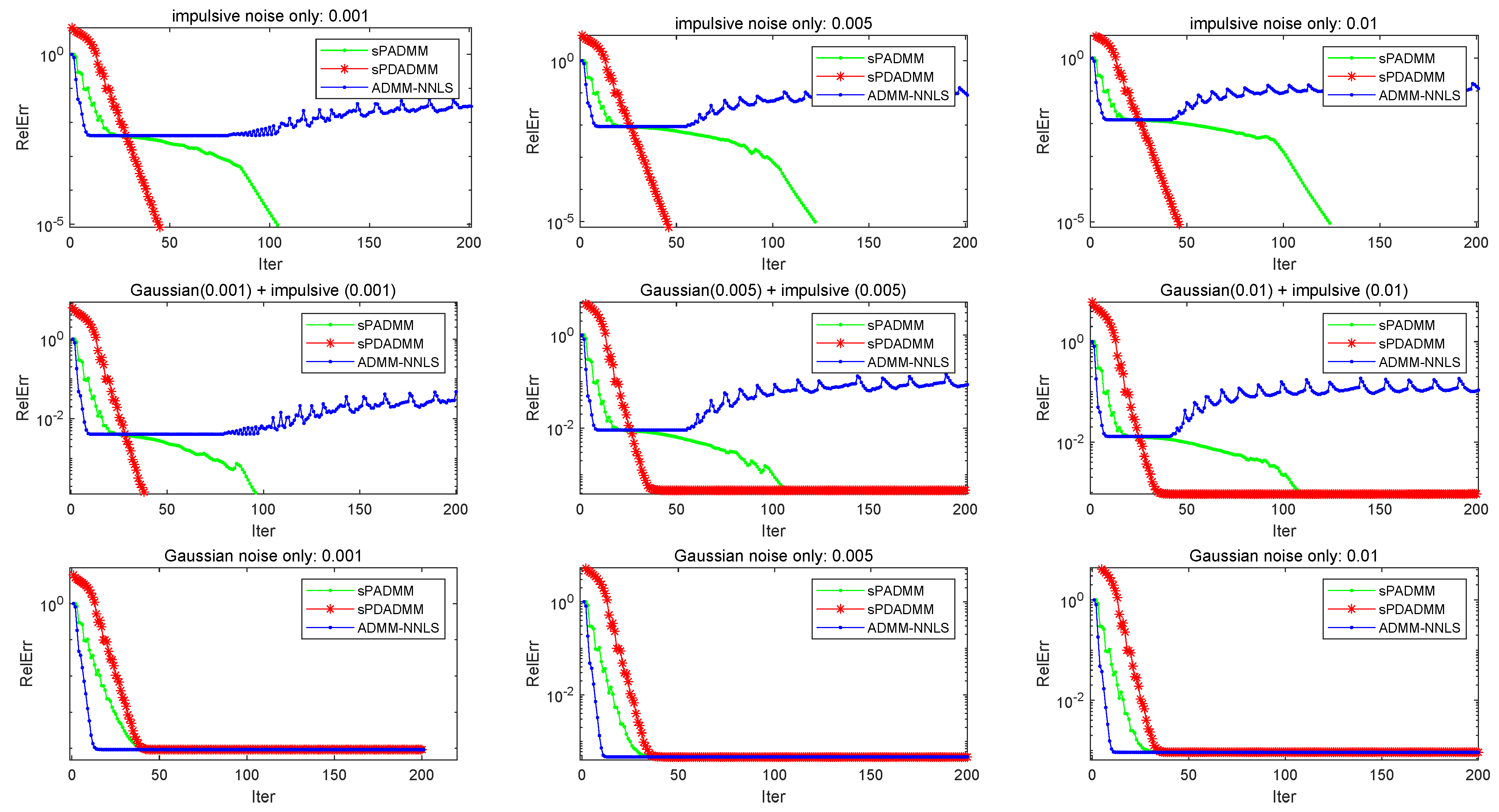
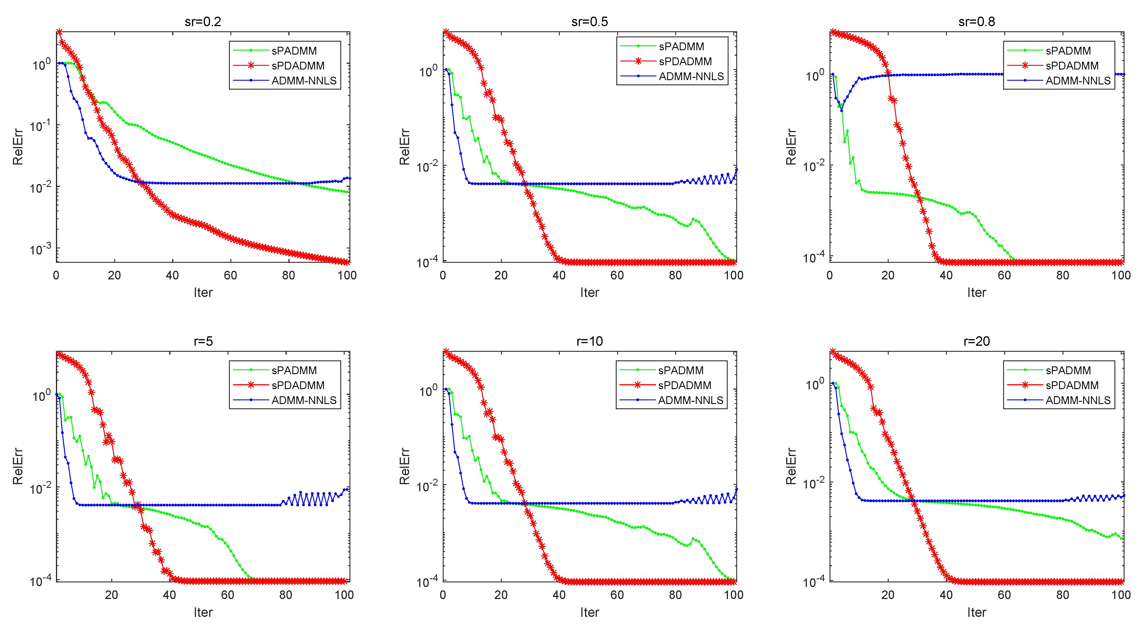
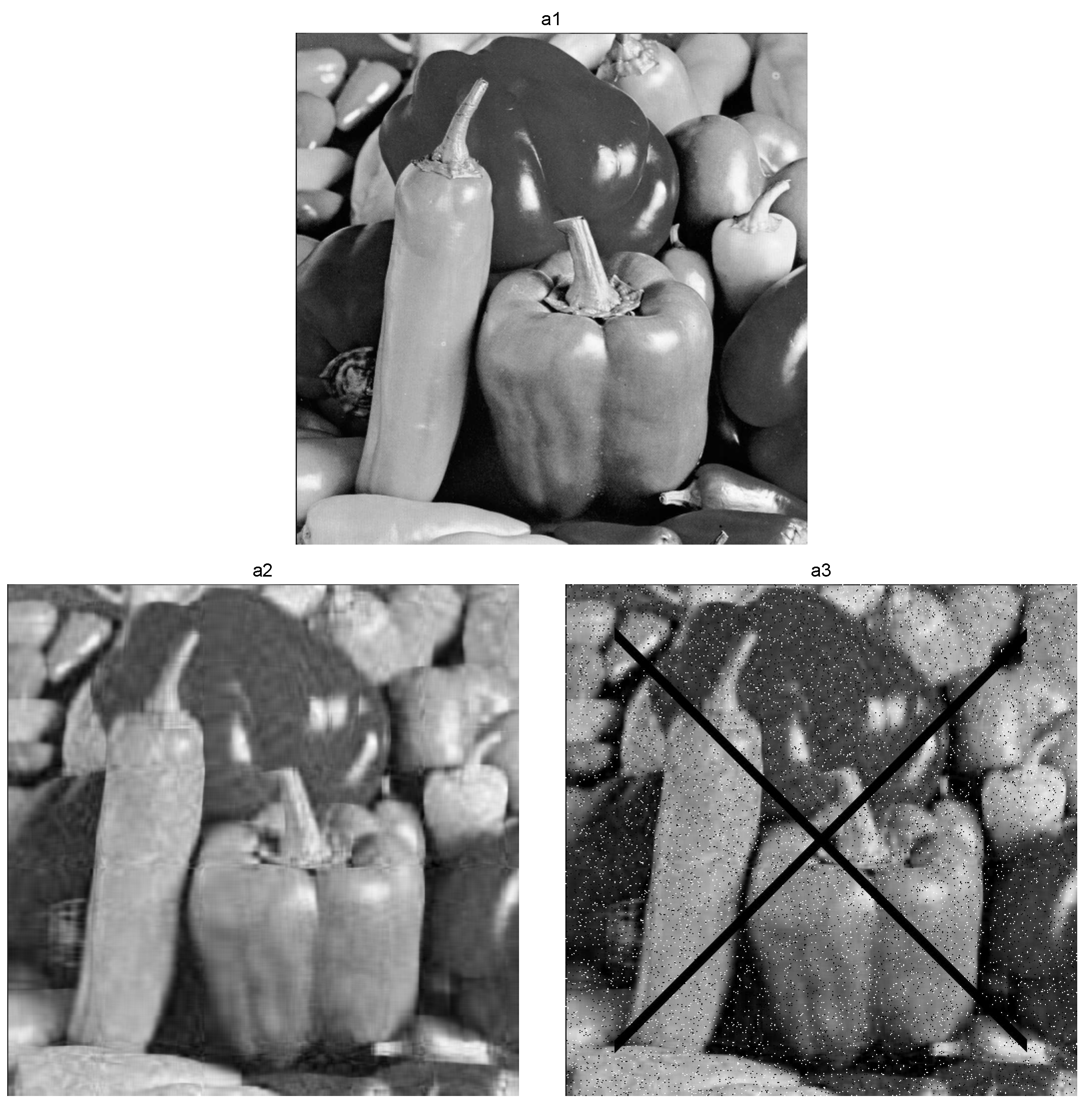
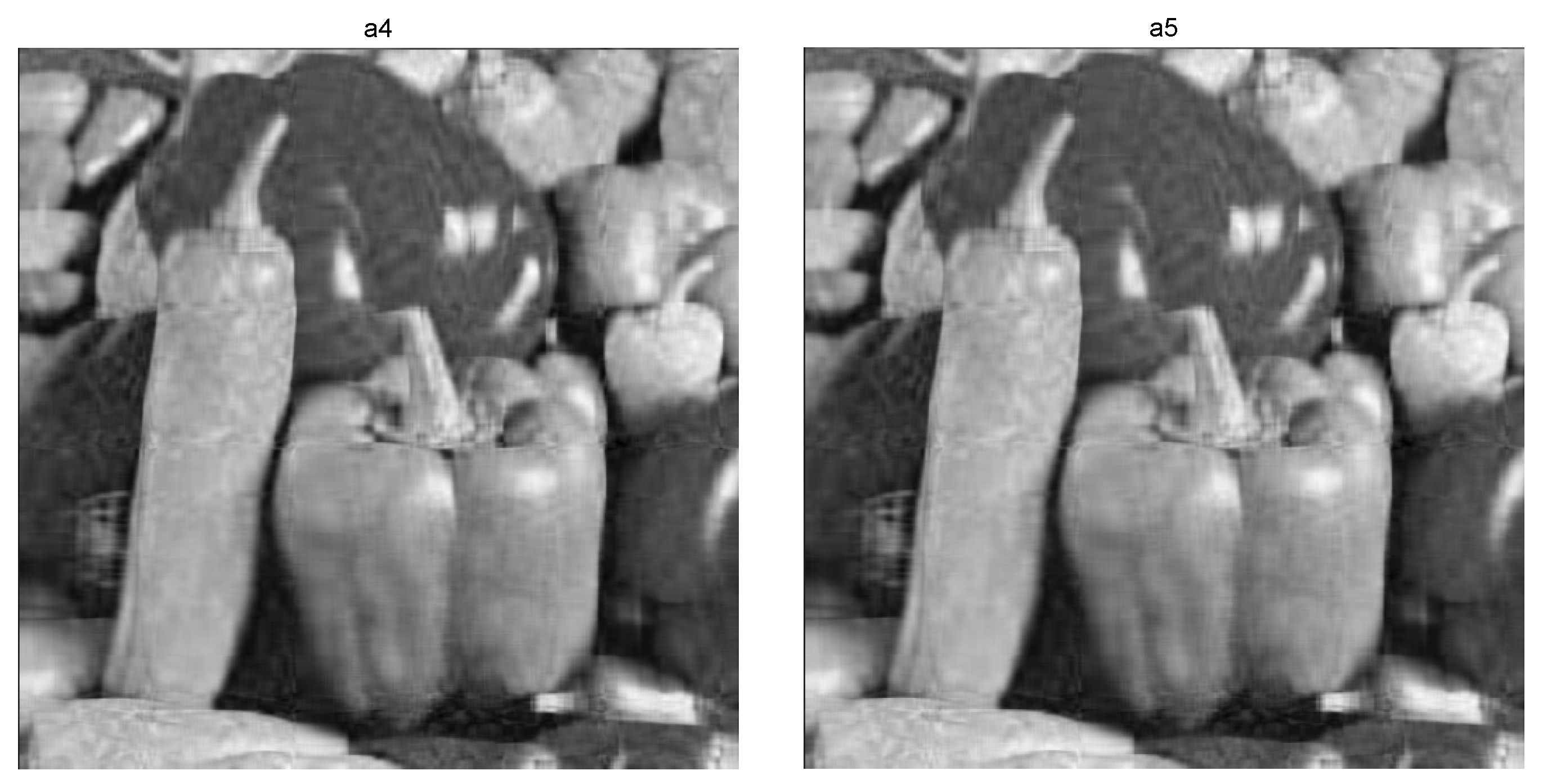
4. Numerical Experiments

In this section, we will have a discussion to emphasize an important issue on choosing denoising models for recovering a low-rank matrix. In many practical applications, measured data are usually contaminated by different kinds of noise or their mixtures. It is well known that models (4) and (5) are widely used to solve the matrix rank minimization problem with noise. Both of them apply the $l_2$-norm for the data-fitting term and usually deal with the problems with Gaussian noise successfully, except non-Gaussian noise.

Thus, in this section, by carrying out kinds of numerical experiments, we demonstrate that model (6) with $l_1$ fidelity can handle several noise cases and perform better than the models with $l_2$ fidelity, and the proposed algorithms can solve the primal and dual problems with approximately precise fidelity.

Now, we firstly give some parameter selections, the meaning of signs, the stopping criterion, and the running environment as follows. m and n denote the row number and the column number of the matrix, respectively. r denotes the rank of the original matrix, which is far less than $min\{m,n\}$. Let $sr$ and p be the sample ratio and the number of measurements, respectively, where p is set to be $p=sr\times m\times n$. Let $dr$ be the number of the degree of freedom for a real-valued rank r matrix, which is $dr=r(m+n-r)$. We note M as the real low-rank matrix, which is generated by $M=M_L{M}_R^T$, where the matrices $M_L\in {\mathbb{R}}^{m\times r}$ and $M_R\in {\mathbb{R}}^{n\times r}$ are generated with independent identically distributed Gaussian entries. The M is produced by the Matlab script “$randn(m,r)\times randn(r,n)$”. $\mathrm{\Omega }$ is an index set of known elements for the matrix completion problem, which are selected uniformly at random entries from $\left\{\right(i,j):i=1,···,m,j=1,···,n\}$. A linear map $\mathcal{A}$ in the general matrix rank minimization usually is the partial discrete cosine transform (PDCT) operator. b is the given measurement vector, and $b=\mathcal{A}\left(X\right)+\omega$, where $\omega ={\omega }_G+{\omega }_I$ is noise. ${\omega }_G$ denotes a Gaussian noise of mean zero and standard deviation $\sigma$, and it can be generated by ${\omega }_G=\sigma \times randn(p,1)$. ${\omega }_I$ represents an impulsive noise, which can be set to $\pm 1$ at N random positions of b, where $N=m\times n\times q$, and $q=0.01,0.005,0.001$ can be chosen, respectively. $\nu$ is an exact penalty parameter, which can be chosen to be slightly greater than the reciprocal of its corresponding Lagrangian multiplier. $\tau$ and $\kappa$ are approximate parameters. We can note that $\rho \left({\mathcal{A}}^{\ast }\mathcal{A}\right)=1$ for matrix completion problems and PDCT measurements. However, we set $\tau ,\kappa =1.1$ because the values of them are slightly greater than $\rho \left({\mathcal{A}}^{\ast }\mathcal{A}\right)$ can accelerate the convergence rate by experiments, which can also be seen in [17]. Let $X^{\ast }$ represent the optimal solution produced by the proposed method.

Now, we terminate the process when the optimal solution $X^{\ast }$ produced by the proposed method satisfies the following criterion

$$RelErr=\frac{\parallel X^{\ast }{-M\parallel }_F}{{\parallel M\parallel }_F}\le tol,$$

(31)

where the relative error measures the quality of $X^{\ast }$ to the original M. The M is recovered successfully by $X^{\ast }$ if the corresponding $RelErr$ is less than ${10}^{-3}$, which has been used in [7,13,38]. So, we usually take the $tol={10}^{-5}$ and the maximum iteration as the terminal condition.

As we noted, the computation of the matrix singular value decomposition (SVD) is needed at each iteration for nuclear norm minimization problems, which may be expensive. So, for all the tests, we apply a PROPACK package [39] for partial SVD. However, PROPACK cannot automatically compute only those singular values greater than a threshold; it needs us to choose the predetermined number $s{v}^k$ of the singular values to be computed at the k-th iteration. As in [14], initializing $s{v}_0=min(m,n)/20$, if $sv{p}_k<s{v}_k$, we set $s{v}_{k+1}=sv{p}_k+1$; if $sv{p}_k=s{v}_k$, we obtain $s{v}_{k+1}=sv{p}_k+5$, where $sv{p}_k$ represents the number of positive singular values of the matrix.

All the experiments are performed under Windows 10 premium and MATLAB R2021a running on a Lenovo laptop with an Intel core CPU at 4.6 GHz and 32 GB memory.

4.1. Matrix Completion Problems

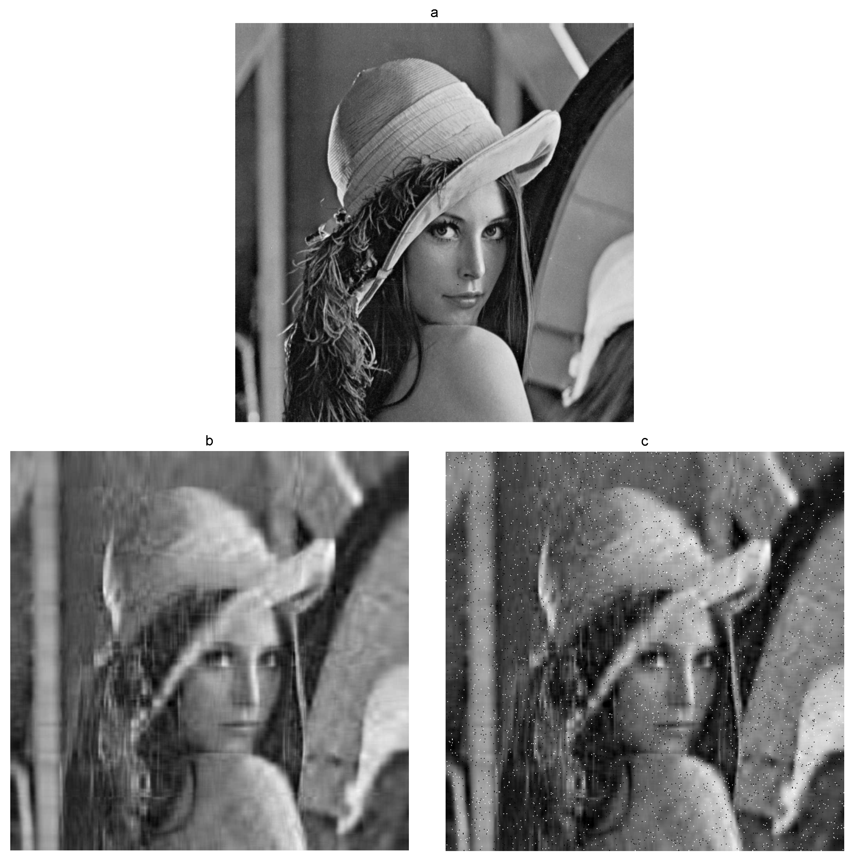
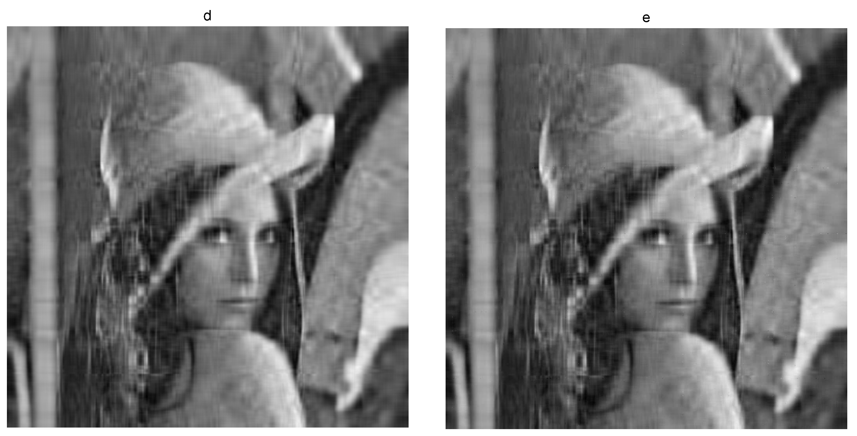
In this subsection, we mainly solve the nuclear norm matrix completion problems with different kinds of noise in order to show their properties for different noisy models. Numerical experiments are tested for solving the following two matrix completion problems. One is the following nuclear norm matrix completion problem with $l_1$ fidelity

$$\underset{X\in {\mathbb{R}}^{m\times n}}{min}{\parallel X\parallel }_{\ast }+\frac{1}{\nu }\sum _{(i,j)\in \mathrm{\Omega }}|X_{i,j}-M_{i,j}|.$$

(32)

Another is the following nuclear norm matrix completion problem with $l_2$ fidelity

$$\underset{X\in {\mathbb{R}}^{m\times n}}{min}{\parallel X\parallel }_{\ast }+\frac{\mu }{2}\sum _{(i,j)\in \mathrm{\Omega }}{|X_{i,j}-M_{i,j}|}^2.$$

(33)

In the following tests, we use the proposed sPADMM and the sPDADMM to solve model (32). Model (33) is solved by the state-of-the-art algorithm ADMM-NNLS [17].

Test 1: The numerical results can be seen in Figure 1. We test the two problems (32) and (33) with three noisy cases: impulsive noise only, Gaussian and impulsive noise, and Gaussian noise only. Moreover, we choose the maximum iteration to be 200 and $tol={10}^{-5}$ as the stopping rule in order to observe their performance more clearly.

From the first row of Figure 1, we can see that the proposed sPADMM and sPDADMM for model (32) can obtain a higher accuracy than the ADMM-NNLS for model (33). Moreover, the sPDADMM can attain accuracy faster than the sPADMM. Observing the second row, it is the case containing both Gaussian and impulsive noises. It is clear to see that using model (32) can recover the matrix successfully; however, model (33) is inefficient only if the measurement contains a little impulsive noise. In other words, no matter how small the percentage of impulsive noise contained in the measurement b, model (32) performs better than model (33). In the third row, we test the case with Gaussian noise only, where the noisy level $\sigma$ varies from $0.001$ to $0.01$. From the bottom row of Figure 1, we can see that model (33) obtains a faster convergence rate than model (32) and attains a similar accuracy of the solution as model (32). Additionally, it is illustrated that model (33) can efficiently solve the case of containing Gaussian noise only, but the proposed model (32) is more efficient and robust for the case with non-Gaussian noise.

To sum up, these numerical results illustrate the following conclusions for the nuclear norm minimization problem. Firstly, whenever the observation data contain impulsive noise, Gaussian noise, or their mixtures, model (32) naturally performs better than model (33) or its variants. In particular, the data with impulsive noise only can be recovered exactly by using model (32) as the parameter chosen appropriately, but model (33) is inefficient. Secondly, without impulsive noise, the $l_1$-fitting model (32) does not harm the quality of the solution as long as the measurement data do not contain a large amount of Gaussian noise. The above analysis illustrates that model (32) has a broader scope of applicability. Finally, when the data contain a large amount of Gaussian noise, the $l_2$-fitting model (33) performs better, but high accuracy would not be obtained no matter which method is chosen.

Test 2: The numerical results can be seen in Figure 2. This test mainly observes the performances of models (32) and (33) with different $sr$ and r, which all contain both Gaussian noise ($\sigma =0.001$) and impulsive noises ($q=0.001$).

From the first row of Figure 2, we can see that model (32) may perform better than model (33) for the matrix completion problem with mixture noises when the $sr$ is relatively higher. Observing the second row of Figure 2, it is clear to see that both the sPADMM and sPDADMM for (32) perform well with r increasing. Moreover, model (32) can obtain a higher accuracy within 100 iterations than model (33). The above numerical analysis shows the robustness of model (32) and the efficiency of the proposed algorithms.

Test 3: The numerical results on recovering real gray images can be seen in Figure 3, which is a $512\times 512$ image. Firstly, we apply matrix SVD for obtaining the low-rank images. Then, we randomly select $60\%$ of the elements from the low-rank image and add some different kinds of noise to obtain the corrupted images. Finally, the corrupted images are recovered by using the proposed sPADMM and sPDADMM to solve model (32). Here, we also use the $RelErr$ to measure the quality of the recovered images.

From the (d) and (e) in Figure 3, we can see that the proposed sPADMM and sPDADMM recovered the corrupted image with impulsive noise and Gaussian noise successfully. In the same way, the (a4) and (a5) in Figure 4 show that the sPADMM and sPDADMM can recover the corrupted image without randomly selecting samples, which also contains only impulsive noise. In a word, these tests show that the proposed sPADMM and sPDADM perform well on recovering these real corrupted images.

4.2. Nuclear Norm Minimization with $l_1$ Fidelity Term

In this subsection, we mainly describe some results of the sPADMM and sPDADMM for solving the problem (6) to illustrate the robustness of model (6) and the efficiency of the sPADMM and sPDADMM.

Test 4: The numerical results are shown in

Table 1. Numerical results of sPADMM and sPDADMM for problem (6), $m=n , sr = 0.5,q = 0.005$.

		sPADMM			sPDADMM
$(\mathit{m},\mathit{r})$	p/dr	Iter	Time	RelErr	Iter	Time	RelErr
(100, 5)	5.13	117	0.77	$9.48\times {10}^{-6}$	85	0.20	$9.35\times {10}^{-6}$
(200, 5)	10.13	85	0.77	$9.03\times {10}^{-6}$	43	0.39	$8.26\times {10}^{-6}$
(400, 5)	20.13	91	3.19	$9.01\times {10}^{-6}$	50	2.22	$8.63\times {10}^{-6}$
(600, 5)	30.13	91	7.88	$8.56\times {10}^{-6}$	50	7.18	$9.04\times {10}^{-6}$
(800, 5)	40.13	88	16.41	$9.41\times {10}^{-6}$	52	16.06	$7.65\times {10}^{-6}$
(1000, 5)	50.13	90	34.09	$9.20\times {10}^{-6}$	54	31.68	$9.35\times {10}^{-6}$
(1200, 10)	30.13	35	39.91	$7.62\times {10}^{-6}$	74	112.76	$8.38\times {10}^{-6}$
(1400, 10)	35.13	34	61.55	$9.72\times {10}^{-6}$	41	62.03	$9.24\times {10}^{-6}$
(1600, 10)	45.13	34	67.11	$9.11\times {10}^{-6}$	41	150.57	$9.55\times {10}^{-6}$
(1800, 10)	50.13	34	100.97	$8.40\times {10}^{-6}$	40	235.03	$8.33\times {10}^{-6}$
(2000, 10)	50.13	34	135.99	$8.90\times {10}^{-6}$	41	316.22	$9.49\times {10}^{-6}$

. We test the sPADMM and sPDADMM for solving (6) with impulsive noise.

From Table 1, we can see that all the situations can be recovered successfully and attain high accuracy, which can be reviewed as successful recovery. In addition, the sPDADMM is faster than the sPADMM as the scale is smaller. When the scale becomes larger, the Z-subproblem needs to compute a full SVD, so it becomes expensive. Moreover, we can solve some larger-scale problems if the CPU memory capacity is large enough. These limited numerical results illustrate that the proposed sPADMM and sPDADMM are very efficient for solving the nuclear norm minimization problem with impulsive noise.

Test 5: The numerical results can be seen in

Table 2. Numerical results of sPADMM and sPDADMM for (6), $m = n,sr = 0.5$.

				sPADMM			sPDADMM
$(\mathit{m},\mathit{r})$	p/dr	q	$\mathbf{\sigma }$	Iter	Time	RelErr	Iter	Time	RelErr
(500, 10)	15.15	0.1	0.00	200	55.28	$2.69\times {10}^{20}$	67	13.33	$9.58\times {10}^{-6}$
(500, 10)	15.15	0.05	0.00	200	87.26	$1.67\times {10}^{-4}$	62	11.90	$9.14\times {10}^{-6}$
(500, 10)	15.15	0.01	0.00	122	13.02	$8.79\times {10}^{-6}$	56	10.04	$8.86\times {10}^{-6}$
(500, 10)	15.15	0.005	0.00	111	13.01	$9.72\times {10}^{-6}$	55	9.57	$9.54\times {10}^{-6}$
(500, 10)	15.15	0.001	0.00	104	11.41	$9.82\times {10}^{-6}$	55	9.64	$8.22\times {10}^{-6}$
(500, 10)	15.15	0.001	0.001	200	23.85	$9.34\times {10}^{-4}$	200	42.50	$2.61\times {10}^{-3}$
(500, 10)	15.15	0.005	0.005	200	26.52	$4.65\times {10}^{-4}$	200	35.01	$1.24\times {10}^{-3}$
(500, 10)	15.15	0.01	0.01	200	21.54	$9.25\times {10}^{-5}$	200	37.50	$1.02\times {10}^{-4}$
(500, 10)	15.15	0.00	0.01	200	45.33	$9.26\times {10}^{-4}$	200	69.90	$2.49\times {10}^{-3}$
(500, 10)	15.15	0.00	0.00	54	5.03	$8.84\times {10}^{-6}$	55	11.12	$8.22\times {10}^{-6}$

. In order to further illustrate the efficiency of the sPADMM and sPDADMM and the robustness of the proposed model, we test the sPADMM and sPDADMM to solve the problem (6) with different noises, which are impulsive noise, Gaussian noise, and their mixtures, respectively. Here, we set the terminated conditions to be $tol={10}^{-5}$ and $maxiter=200$.

From Table 2, we can observe that the proposed sPADMM can successfully solve almost all problems, except the case with only impulsive noise ($q=0.1$). The mentioned case $q=0.1$ is a highly challenging problem because the noise level is so high. But the proposed sPDADMM can successfully deal with all the cases; moreover, it can attain high accuracy in the case of only impulsive noise ($q=0.1$). Additional experiments are conducted in the following

Table 3. Numerical results of sPADMM and sPDADMM for (6), $m=n$.

				sPADMM			sPDADMM
$(\mathit{m},\mathit{r})$	sr	q	$\mathbf{\sigma }$	Iter	Time	RelErr	Iter	Time	RelErr
(500, 5)	0.3	0.1	0.00	200	96.72	$1.34\times {10}^{14}$	200	56.37	$1.46\times {10}^{-1}$
(500, 5)	0.5	0.1	0.00	200	94.05	$4.84\times {10}^{14}$	56	13.05	$9.01\times {10}^{-6}$
(500, 5)	0.8	0.1	0.00	101	17.14	$8.85\times {10}^{-6}$	25	5.11	$6.98\times {10}^{-6}$
(500, 10)	0.3	0.1	0.00	200	72.28	$3.33\times {10}^{15}$	200	45.17	$1.26\times {10}^{-1}$
(500, 10)	0.5	0.1	0.00	200	55.28	$2.69\times {10}^{20}$	67	13.33	$9.58\times {10}^{-6}$
(500, 10)	0.8	0.1	0.00	156	121.12	$9.45\times {10}^{-6}$	27	6.29	$8.48\times {10}^{-6}$

for illustrating the aforementioned results. The sampling rate $sr$ has a great influence on whether the problem can be solved successfully. Observing the results in Table 3, the sPADMM cannot be successfully implemented for the cases of $sr\le 0.5,q=0.1$. As the sampling rate increases, so does the efficiency of both algorithms. Moreover, the sPDADMM can solve successfully for the case of $sr=0.5$ and is superior to the sPADMM for all the cases. These numerical results illustrate that the sPDADMM for solving the dual problem of (6) is more robust, which is our main contribution to apply an effective and robust method for solving the nonsmooth convex optimization problem (6) from the dual perspective. As the level of the Gaussian noise becomes high, it can be seen that the sPADMM can obtain higher accuracy than the sPDADMM. Especially, both of the proposed algorithms are efficient for the noiseless case.

Test 6: The numerical results are displayed in Figure 5. We test the sPADMM and sPDADMM for solving problem (6) with different $sr$.

Observing Figure 5, we can see that the sPADMM and sPDADMM perform better with $sr$ increasing and can even attain a higher accuracy than ${10}^{-12}$. In the meantime, as the parameter is chosen appropriately, it can obtain an approximate exact solution for solving the matrix nuclear norm minimization problem.

These numerical results show that the above conclusions on the matrix completion problem (32) also apply to the general problem (6) as well. Moreover, if the measurement contains kinds of noises, it is more efficient to choose the nuclear norm minimization problem with the $l_1$-norm fidelity term. Moreover, these tests illustrate that the sPADMM is more robust and efficient for solving the case with non-Gaussian noise.

5. Conclusions

In this paper, we proposed some efficient algorithms for solving the nuclear norm minimization problem with the $l_1$-norm fidelity term, which is suitable for recovering a corrupted low-rank matrix with impulsive noise. Especially, when the parameter is chosen appropriately, this proposed model is an exact penalty function problem. We applied the sPADMM for solving it and gave some convergence analyses. Moreover, we first proposed the semi-proximal ADMM for solving the dual problem and gained a more efficient and robust algorithm. Finally, we presented some numerical experiments to illustrate the efficiency of the proposed models and algorithms. The numerical results show that the proposed $l_1$ fidelity model is preferred over the $l_2$ one when the data contain some impulsive noise or the mixture with Gaussian noise. What is more, it is also competitive to the model with $l_2$ fidelity for the noiseless case. In particular, comparing the sPADMM with the sPDADMM, we have noted that the sPADMM is less efficient than the sPDADMM for the problem with the same level of impulsive noise. But as the scale gets larger, a quicker computation of the SVD needs to be introduced for solving the Z-subproblem. Therefore, we will accelerate the sPDADMM by introducing or designing a more efficient method to compute the SVD in the future. Given proper nonconvex regularization achieves a better low-rank estimation and is more robust to noise than the nuclear norm convex relaxation, we will focus on designing efficient algorithms for solving the nonconvex robust low-rank matrix estimation problems with non-Gaussian noise.

References

1. Srebro, N. Learning with Matrix Factorizations. Ph.D. Thesis, MIT Computer Science & Artificial Intelligence Laboratory, Cambridge, MA, USA, 2004. [Google Scholar]
2. Mohan, K.; Fazel, M. Reweighted nuclear norm minimization with application to system identification. In Proceedings of the American Control Conference (ACC), Baltimore, MD, USA, 30 June–2 July 2010; pp. 2953–2959. [Google Scholar]
3. Candès, E.J.; Li, X.; Ma, Y.; Wright, J. Robust principal component analysis? J. ACM (JACM) 2011, 58, 11. [Google Scholar] [CrossRef]
4. Elsener, A.; van de Geer, S. Robust low-rank matrix estimation. Ann. Stat. 2018, 46, 3481–3509. [Google Scholar] [CrossRef]
5. Fazel, M.; Hindi, H.; Boyd, S. Rank minimization and applications in system theory. In Proceedings of the American Control Conference, Boston, MA, USA, 30 June–2 July 2004; Volume 4, pp. 3273–3278. [Google Scholar]
6. Jiang, W.; Wu, D.; Dong, W.; Ding, J.; Ye, Z.; Zeng, P.; Gao, Y. Design and validation of a non-parasitic 2R1T parallel hand-held prostate biopsy robot with remote center of motion. J. Mech. Robot. 2024, 16, 051009. [Google Scholar] [CrossRef]
7. Ma, S.; Goldfarb, D.; Chen, L. Fixed point and Bregman iterative methods for matrix rank minimization. Math. Program. 2011, 128, 321–353. [Google Scholar] [CrossRef]
8. Candès, E.J.; Recht, B. Exact matrix completion via convex optimization. Found. Comput. Math. 2009, 9, 717–772. [Google Scholar] [CrossRef]
9. Candès, E.J.; Tao, T. The power of convex relaxation: Near-optimal matrix completion. IEEE Trans. Inf. Theory 2010, 56, 2053–2080. [Google Scholar] [CrossRef]
10. Keshavan, R.H.; Montanari, A.; Oh, S. Matrix completion from a few entries. IEEE Trans. Inf. Theory 2010, 56, 2980–2998. [Google Scholar] [CrossRef]
11. Sturm, J.F. Using SeDuMi 1.02, a MATLAB toolbox for optimization over symmetric cones. Optim. Methods Softw. 1999, 11, 625–653. [Google Scholar] [CrossRef]
12. Tütüncü, R.H.; Toh, K.C.; Todd, M.J. Solving semidefinite-quadratic-linear programs using SDPT3. Math. Program. 2003, 95, 189–217. [Google Scholar] [CrossRef]
13. Cai, J.F.; Candès, E.J.; Shen, Z. A singular value thresholding algorithm for matrix completion. SIAM J. Optim. 2010, 20, 1956–1982. [Google Scholar] [CrossRef]
14. Toh, K.C.; Yun, S. An accelerated proximal gradient algorithm for nuclear norm regularized linear least squares problems. Pac. J. Optim. 2010, 6, 615–640. [Google Scholar]
15. Liu, Y.J.; Sun, D.; Toh, K.C. An implementable proximal point algorithmic framework for nuclear norm minimization. Math. Program. 2012, 133, 399–436. [Google Scholar] [CrossRef]
16. Xiao, Y.H.; Jin, Z.F. An alternating direction method for linear-constrained matrix nuclear norm minimization. Numer. Linear Algebra Appl. 2012, 19, 541–554. [Google Scholar] [CrossRef]
17. Yang, J.; Yuan, X. Linearized augmented Lagrangian and alternating direction methods for nuclear norm minimization. Math. Comput. 2013, 82, 301–329. [Google Scholar] [CrossRef]
18. Ding, Y.; Xiao, Y. Symmetric Gauss–Seidel technique-based alternating direction methods of multipliers for transform invariant low-rank textures problem. J. Math. Imaging Vis. 2018, 60, 1220–1230. [Google Scholar] [CrossRef]
19. Micchelli, C.A.; Shen, L.; Xu, Y.; Zeng, X. Proximity algorithms for the L1/TV image denoising model. Adv. Comput. Math. 2013, 38, 401–426. [Google Scholar] [CrossRef]
20. Alliney, S. A property of the minimum vectors of a regularizing functional defined by means of the absolute norm. IEEE Trans. Signal Process. 1997, 45, 913–917. [Google Scholar] [CrossRef]
21. Udell, M.; Horn, C.; Zadeh, R.; Boyd, S. Generalized low rank models. Found. Trends® Mach. Learn. 2016, 9, 1–118. [Google Scholar] [CrossRef]
22. Zhao, L.; Babu, P.; Palomar, D.P. Efficient algorithms on robust low-rank matrix completion against outliers. IEEE Trans. Signal Process. 2016, 64, 4767–4780. [Google Scholar] [CrossRef]
23. Jiang, X.; Zhong, Z.; Liu, X.; So, H.C. Robust matrix completion via alternating projection. IEEE Signal Process. Lett. 2017, 24, 579–583. [Google Scholar] [CrossRef]
24. Guennec, A.; Aujol, J.; Traonmilin, Y. Adaptive Parameter Selection for Gradient-Sparse + Low Patch-Rank Recovery: Application to Image Decomposition. HAL Id: Hal-04207313. 2024. Available online: https://hal.science/hal-04207313/document (accessed on 17 March 2023).
25. Liang, W. Alternating Direction Method of Multipliers for Robust Low Rank Matrix Completion. Ph.D. Thesis, Beijing Jiaotong University, Beijing, China, 2020. [Google Scholar]
26. Wong, R.K.W.; Lee, T.C.M. Matrix completion with noisy entries and outliers. J. Mach. Learn. Res. 2017, 18, 5404–5428. [Google Scholar]
27. Abreu, E.; Lightstone, M.; Mitra, S.K.; Arakawa, K. A new efficient approach for the removal of impulse noise from highly corrupted images. IEEE Trans. Image Process. 1996, 5, 1012–1025. [Google Scholar] [CrossRef] [PubMed]
28. Ji, H.; Liu, C.; Shen, Z.; Xu, Y. Robust video denoising using low rank matrix completion. In Proceedings of the Computer Vision and Pattern Recognition (CVPR), San Francisco, CA, USA, 13–18 June 2010; pp. 1791–1798. [Google Scholar]
29. Wang, D.; Jin, Z.F.; Shang, Y. A penalty decomposition method for nuclear norm minimization with l1 norm fidelity term. Evol. Equ. Control Theory 2019, 8, 695–708. [Google Scholar] [CrossRef]
30. Rockafellar, R.T. Convex Analysis; Princeton University Press: Princeton, NJ, USA, 1970. [Google Scholar]
31. Parikh, N.; Boyd, S. Proximal algorithms. Found. Trends® Optim. 2014, 1, 127–239. [Google Scholar] [CrossRef]
32. Xiao, Y.; Zhu, H.; Wu, S.Y. Primal and dual alternating direction algorithms for l1-l1-norm minimization problems in compressive sensing. Comput. Optim. Appl. 2013, 54, 441–459. [Google Scholar] [CrossRef]
33. Jiang, K.; Sun, D.; Toh, K.C. A partial proximal point algorithm for nuclear norm regularized matrix least squares problems. Math. Program. Comput. 2014, 6, 281–325. [Google Scholar] [CrossRef]
34. Glowinski, R.; Marroco, A. Sur l’approximation, paréléments finis d’ordre un, et la résolution, par pénalisation-dualité d’une classe de problémes de Dirichlet non linéaires. ESAIM Math. Model. Numer.-Anal.-Modél. Math. Anal. Numér. 1975, 9, 41–76. [Google Scholar]
35. Gabay, D.; Mercier, B. A dual algorithm for the solution of nonlinear variational problems via finite element approximation. Comput. Math. Appl. 1976, 2, 17–40. [Google Scholar] [CrossRef]
36. Eckstein, J. Some Saddle-function splitting methods for convex programming. Optim. Methods Softw. 1994, 4, 75–83. [Google Scholar] [CrossRef]
37. Fazel, M.; Pong, T.K.; Sun, D.; Tseng, P. Hankel matrix rank minimization with applications to system identification and realization. SIAM J. Matrix Anal. Appl. 2013, 34, 946–977. [Google Scholar] [CrossRef]
38. Jin, Z.F.; Wan, Z.; Zhao, X.; Xiao, Y. A Penalty Decomposition Method for Rank Minimization Problem with Affine Constraints. Appl. Math. Model. 2015, 39, 4859–4870. [Google Scholar] [CrossRef]
39. Larsen, R.M. PROPACK-Software for Large and Sparse SVD Calculations. 2004. Available online: http://sun.stanford.edu/~rmunk/PROPACK/ (accessed on 17 March 2004).
Figure 1. Numerical comparisons of models (32) and (33) (m = n = 500, r = 10, and sr = 0.5). First row: impulsive noise only (from left to right, q is 0.001 , 0.005 , and 0.01 , respectively); second row: Gaussian and impulsive noise; third row: Gaussian noise only (from left to right, σ is 0.001 , 0.005 , and 0.01 , respectively).
Symmetry 16 00303 g001
Figure 2. Numerical comparative results of models (32) and (33) ( m = n = 500 ). First row: r = 10 , and s r is 0.2 , 0.5 , 0.8 , respectively. Second row: s r = 0.5 , and r is 5 , 10 , 20 , respectively.
Symmetry 16 00303 g002
Figure 3. (a) Original gray image ( 512 × 512 ); (b) corresponding low-rank images with r = 20 ; (c) randomly masked image from rank 20 with s r = 60 % , σ = 0.001 , and q = 0.02 ; (d) recovered images by the sPADMM, whose “RelErr” is 3.10 × 10 3 ; and (e) recovered images by the sPDADMM, whose “RelErr” is 9.71 × 10 3 .
Symmetry 16 00303 g003aSymmetry 16 00303 g003b
Figure 4. (a1) Original gray image ( 512 × 512 ); (a2) corresponding low-rank images with r = 30 ; (a3) randomly masked image from rank 30 with q = 0.02 ; (a4) recovered images by sPADMM; and (a5) recovered images by sPDADMM.
Symmetry 16 00303 g004aSymmetry 16 00303 g004b
Figure 5. sPADMM (left) and sPDADMM (right) for problem (6) with impulsive noise: m = n = 500; r = 10; sr = 0.2, 0.4, 0.6, and 0.8; and q = 0.005.
Symmetry 16 00303 g005