Abstract
Fermatean fuzzy sets (FFSs) serve as a nascent yet potent approach for coping with fuzziness, with their efficacy recently being demonstrated across a spectrum of practical contexts. Nevertheless, the scholarly literature remains limited in exploring the similarity and distance measures tailored for FFSs. The limited existing measures on FFSs sometimes yield counter-intuitive outcomes, which can obfuscate the accurate quantification of similarity and difference among FFSs. This paper introduces a suite of similarity and distance measures tailored for FFSs, drawing inspiration from the Tanimoto measure. We delve into the characteristics of these novel measures and offer some comparative studies with existing FFSs measures, highlighting their superior efficacy in the processing of fuzzy data from FFSs. Our proposed measures effectively rectify the counter-intuitive situations encountered with many existing measures and demonstrate a significant enhancement in differentiating between diverse FFSs. Moreover, we showcase the real-world applicability of our proposed measures through case studies in pattern recognition, medical diagnostics, and multi-attribute decision-making.
1. Introduction
The increasing prevalence of uncertainty across diverse disciplines is a direct consequence of the intricate nature of objective realities and the bounds of human cognition [1,2,3]. Fuzziness manifests as a type of uncertainty arising from imprecise or vague information, being one of the specific forms of uncertainty. This nebulous characteristic often manifests itself in a probabilistic and indeterminate manner, which challenges the pursuit of precise delineations. In response, the scholarly community has developed a multitude of innovative theories and methodologies to effectively encapsulate and address the fuzziness within practical contexts [4,5,6,7,8]. Among these, fuzzy sets theory, introduced by Zadeh in 1965 [4], has garnered substantial scholarly focus. This theory broadens the scope of classical set theory to accommodate scenarios where categorical boundaries are not clearly demarcated. By assigning membership values to elements within a set, fuzzy sets facilitate a nuanced and more precise representation of ambiguous concepts. Fuzzy sets theory revolutionizes traditional decision-making paradigms by enabling reasoning based on fuzzy information and decisions informed by partial or ambiguous data. This innovative approach has been instrumental in modeling and articulating fuzzy and uncertain information, and its utility has been widely recognized in domains such as pattern recognition, signal processing, medical diagnosis, and inference systems [9,10,11,12,13,14,15].
In the context of increasingly intricate decision-making scenarios, the common theory of fuzzy sets encounters its bounds in the precise depiction of uncertain data. To rectify this shortcoming, academia has championed various enhancements to conventional fuzzy sets, including Intuitionistic fuzzy sets (IFSs) [16], hesitant fuzzy sets [6], evidence theory [17], and rough sets [18]. Notably, IFSs have garnered significant focus, owing to their proficiency in encapsulating both fuzzy and uncertain data by incorporating elements’ membership and non-membership degrees. This distinctive trait has rendered IFSs an indispensable instrument across diverse research fields for tackling uncertainties [19,20,21]. Building upon the foundation of IFSs, in 2013, Yager pioneered the concept of Pythagorean fuzzy sets (PFSs) [22]. This paradigm encompasses a Pythagorean function, amalgamating membership, non-membership, and hesitancy degrees, thus transcending the original confines of membership and non-membership alone. PFSs enforce a constraint such that the cumulative squares of the degrees of membership and non-membership are confined below one, thereby enhancing their capacity to encapsulate and delineate fuzzy information [23,24,25]. However, though IFSs and PFSs have achieved considerable success in handling certain types of uncertainties, they may not always offer sufficient flexibility in certain specific application scenarios. For example, both Intuitionistic fuzzy sets (IFSs) and Pythagorean fuzzy sets (PFSs) are unable to accommodate scenarios where the sum or squared sum of membership and non-membership degrees exceeds unity [26]. To solve this issue, recently, Yager and Filev [27] extended PFSs and introduced a novel type of fuzzy set called Fermatean fuzzy sets (FFSs) in 2019. FFSs is founded on the notion of Fermatean distance, which postulates that the sum of the cubes of the membership and non-membership degrees must not exceed one, and encompasses hesitation in capturing and representing uncertain information. This attribute enables it to encompass a greater amount of information, making it more powerful than PFSs and IFSs. Fermatean fuzzy sets (FFS) enhance the granularity of fuzziness representation by introducing additional parameters and functions, thereby capturing more nuanced information about fuzziness [26]. This fine-grained representation is particularly significant in fields that demand high precision, such as medical diagnostics [28,29] and financial risk assessment [30,31]. Currently, FFSs have evoked considerable interest among researchers. Ghorabaee [32] introduced an innovative decision-making methodology founded on FFSs. Garg [33] demonstrated the utilization of Fermatean fuzzy aggregation functions within COVID-19 testing facilities. Aydemir and Yilmaz [34] introduced a method, known as TOPSIS, to determine preference orders in FFS based on similarity to ideal solutions. Shahzadi and Akram [35] introduced the formation of fuzzy soft sets and demonstrated their utility in selecting appropriate antivirus masks. Gul [36] showed the utility of FFSs in assessing occupational risks within the manufacturing sector. Sergi and Sari [37] proposed some Fermatean fuzzy capital budgeting techniques. Sivadas [38] introduced the Fermatean fuzzy soft set, a novel hybrid structure that amalgamates the features of Fermatean fuzzy sets with the parameterization typical of soft set theory. Ali and Ansari [26] introduced the notion of formation fuzzy bipolar soft sets and demonstrated their applicability in multiple-criteria decision-making (MCDM). In addition, FFSs have also been employed in several fields including data mining, image processing, and clustering [32,39,40,41].
The concepts of similarity measure and distance measure are two other crucial concepts in the theory of fuzzy sets. They, respectively, refer to mathematical functions that evaluate the similarity and distance between two entities based on their distinctive attributes. In classical set theory, similarity is usually quantified using set-theoretic measures, such as Jaccard similarity or cosine similarity [42,43]. However, these measures perform poorly for fuzzy sets because they fail to account for the membership grades associated with constituent elements. The concept of similarity measure is employed to determine the similarity between individuals, while the concept of distance measure is used to quantify the degree of difference between individuals. Similarity measures include broader measures than distance measures, which specifically calculate differences in Cartesian space. These terms are often used interchangeably, with distance often serving as the reciprocal of similarity and vice versa. In terms of evaluation, for distance measure, the shortest distance is observed between the closest points, while for similarity measure, the highest level of similarity is observed between the closest points. Recent research has introduced innovative similarity measures and distance measures:
- Garg [44] has proposed a similarity measure that utilizes transformed right-angled triangles. Huang [45] has presented a novel similarity/distance measure under an Intuitionistic fuzzy environment enhancing its capability to address real-world fuzziness, whereas Olgun [46] has designed an IFSs similarity measure utilizing the framework of Choquet integral, thereby incorporating a modified approach to the cosine metric. Kumar [47] has presented a novel IFSs similarity measure, deployed in applications such as pattern recognition and clustering analysis. Moreover, Duan [48] has presented an innovative Intuitionistic fuzzy similarity measure. Garg [49] developed a novel measure based on PFSs to tackle the challenges associated with multiple-attribute decision-making (MADM). Li [50] introduced a fresh similarity assessment for PFSs, which is founded on the concept of spherical arc distance from a geometric standpoint. Additionally, a MADM approach was established in a Pythagorean fuzzy setting. Hussian and Yang [51] put forward novel similarity measures for PFSs that are grounded in Hausdorff measures. Additionally, recent studies [52,53,54,55,56,57,58] have introduced numerous other similarity measures.
- Atanassov delineated four 2D distance measures, which were established on the foundations of the concepts of Euclidean and Hamming distances [16]. The Hausdorff distance measures were proposed by Glazoczewski [59] to distinguish differences between IFSs. More recently, Gohain put forth a measure that is predicated on the divergence of the maximum and minimal cross-validation indices [60]. Panda and Mahanta introduced a nonlinear distance measure that takes into consideration the discrepancies among IFSs with substantial hesitation levels [61]. Xiao introduced a novel Jensen–Shannon divergence-based IFSs distance measure [62]. Also, Li [63] conducted an inquiry into the normalized Hamming and Euclidean distance, aiming to enhance the precision and computational efficiency of fuzzy set proximity computations. Zeng [64] introduced a novel distance measure for IFSs, thereby extending its utility within the domain of pattern recognition. Talebi utilized a distance measure grounded in -stable statistical models and developed an adaptive filtering structure [65]. Li [66] presented an innovative distance measure under a Pythagorean fuzzy environment, while Xu [67] introduced a measure based on Hamming distance. Furthermore, Gou, Xu, and Ren [68] introduced an innovative distance measure that builds upon the Euclidean distance model for PFSs.
At present, the similarity and distance measures for IFSs and PFSs are relatively complete.
Currently, several similarity and distance measures have been put forward for FFSs, including the new distance using Hellinger distance and triangular divergence [69], the cosine similarity measure by Kirişci [70], the cosine similarity by Sahoo [71] and the similarity measure based on linguistic scale function [72]. These measures are designed to confront issues including complexity, asymmetry, and variations in intersection size. Despite this, there is still limited research on the measures of similarity and distance in FFSs, and the existing measures for FFSs suffer from counter-intuitive outcomes, insufficient sensitivity to varying intersection sizes, and asymmetry issues, which are not applicable under many conditions. Therefore, the study of similarity and distance measures of FFSs has become an important research field with significant academic significance.
This paper introduces a set of novel similarity and distance measures for FFSs. The properties of these measures are thoroughly analyzed through abundant examples. Additionally, we propose two models that employ these measures for tasks, including medical diagnosis, pattern recognition, and MADM problems, within Fermatean fuzzy environments. We present an array of experiments comparing our measures to existing ones. The results demonstrate that our proposed measures overcome numerous counter-intuitive situations, and enhance the dependability of the decision-making process in identifying distinctions among FFSs. These qualities exemplify the superior nature of our proposed measures.
The primary contributions of this study are delineated as follows:
- (1)
- We introduce novel similarity and distance measures for FFSs and provide proofs of their properties.
- (2)
- Two models employing these measures are proposed for medical diagnosis, pattern recognition, and MADM problems, demonstrating their efficacy.
- (3)
- By conducting a comparative evaluation against established measures for FFSs, the measures we suggest exhibit superior performance, with improved sensitivity to discriminating dissimilarities between FFSs and a capacity to circumvent counter-intuitive limitations of existing measures. Our measures offer greater reliability and superiority in distinguishing FFSs.
Section 2 provides a concise overview of the foundational principles underlying fuzzy sets theory. Subsequently, in Section 3, we introduce a suite of innovative similarity and distance measures tailored for FFSs, alongside the delineation of their distinctive attributes. Meanwhile, a large number of experimental studies have been carried out to demonstrate the superiority of the suggested measures in overcoming counter-intuitive situations, distinguishing FFSs, and making more reliable decisions. In Section 4, based on proposed measures, two models are introduced to address medical diagnosis, pattern recognition, and MADM problems. Finally, in Section 5, we draw conclusions and provide directions for subsequent scholarly research.
2. Preliminaries
Within this portion, some foundational concepts related to fuzzy sets, the Tanimoto similarity measure, and several existing measures for FFSs will be provided.
2.1. Intuitionistic Fuzzy Sets
Definition 1
([16]). We utilize the symbol Z to denote a set of limited cardinality. An Intuitionistic fuzzy set I is given by:
Herein, signifies the membership degree of z, and expresses the non-membership degree of z. , and satisfy:
, the indeterminacy degree associated with z is given by:
This definition encapsulates the essence of Intuitionistic fuzzy sets within a finite domain Z.
2.2. Pythagorean Fuzzy Sets
Definition 2
([22]). The Pythagorean fuzzy set P is given by the following representation:
In this construct, and serve as the membership and non-membership degrees of z, respectively, and are mappings from Z to the interval . , and satisfy:
, the indeterminacy degree associated with z is quantified by:
2.3. Fermatean Fuzzy Sets
Definition 3
([27]). The Fermatean fuzzy set F is given by the following representation:
In this construct, and serve as the membership and non-membership degrees of z, respectively, and are mappings from Z to the interval . , and satisfy:
For all z within the set of integers Z, the degree of indeterminacy associated with z is:
2.4. Existing Measures for FFSs
Definition 4.
Suppose two FFSs, , and . The cosine similarity measure relative to F and G is given by:
Definition 5.
Suppose that , and are two FFSs. The Euclidean distance is defined as:
Definition 6.
([70]). Suppose that , and are two FFSs. The new cosine similarity proposed by Kirişci is defined as:
Definition 7.
([71]). Suppose that , and are two FFSs. Several similarities proposed by Sahoo are defined as:
The score function is defined as:
Definition 8.
([69]). Suppose that , and are two FFSs. The Hellinger distance is defined as:
Definition 9.
([69]). Suppose that , and are two FFSs. The triangular divergence distance is defined as:
2.5. Tanimoto Similarity Measure
Definition 10.
([73]). Let A and B represent two sets of probability distributions, respectively, denoted as and . The Tanimoto measure, which quantifies the similarity between A and B, can be given by:
3. Some Novel Tanimoto Similarity Measures and Distance Measures for FFSs
To date, research on the similarity and distance measures of FFSs remains incomplete, and existing measures can sometimes exhibit counter-intuitive, insensitive to changes, or even asymmetric problems in certain scenarios. Consequently, there is a need to propose new measures that can address these issues. The Tanimoto similarity coefficient exhibits prominent advantages in metric properties, such as effective handling of binary features [74], range constraints [74], simplified computation [74,75], sensitivity to small datasets [74,75], broad applicability in domains like chemical informatics and bioinformatics [75,76], and standardization capabilities [75,76]. Therefore, we are dedicated to investigating the integration of the Tanimoto similarity coefficient with FFSs to enhance the control of uncertainties in real-world applications, particularly in the fields of medicine, biology, and decision-making. Within the current segment, we introduce a suite of Tanimoto similarity measures, along with their weighted forms, for FFSs, capitalizing on the Tanimoto similarity measure. We introduce the corresponding distance measures for comparison with established distance measures. The validity of these new measures is confirmed through a series of computational trials. Additionally, we showcase the ability of the newly introduced measures to resolve the paradoxical issues inherent in existing measures and to excel in distinguishing between diverse FFSs, as supported by multiple illustrative instances.
3.1. New Similarity Measures for FFSs
Definition 11.
Let two FFSs and based on a finite set . The Tanimoto similarity measure for the FFSs can be given as:
Theorem 1.
With respect to any two FFSs, F and G, the must satisfy:
- 1.
- ;
- 2.
- ;
- 3.
- , if .
Proof of Theorem 1.
Hence, the demonstrations have been concluded. □
Considering the weights associated with , a weighted Tanimoto similarity measure for FFSs F and G is introduced as follows:
Definition 12.
For , a weight is allocated. The weighted Tanimoto measure can be given by:
In a manner analogous to the demonstration provided for Theorem 1, the following can be derived:
Theorem 2.
With respect to any two FFSs, F and G, the must satisfy:
- 1.
- ;
- 2.
- ;
- 3.
- , if .
Taking into account the indeterminacy degree, the following can be derived:
Definition 13.
For , take the degree of indeterminacy . The measure is given by:
When considering the degree of indeterminacy and the weights of , we can obtain:
Definition 14.
For , take the degree of indeterminacy and the weight . The measure can be defined as:
3.2. New Distance Measures for FFSs
To facilitate comparison with existing distance measures, we propose the distance form for Tanimoto similarity.
Definition 15.
Considering a fixed set , and are two FFSs, the Tanimoto distance is given by:
The larger the is, the larger the disparity between two FFSs.
Theorem 3.
With respect to any two FFSs, F and G, the must satisfy:
- 1.
- ;
- 2.
- ;
- 3.
- , if .
Definition 16.
For , a weight is allocated. The weighted Tanimoto distance can be given by:
Theorem 4.
With respect to any two FFSs, F and G, the must satisfy:
- 1.
- ;
- 2.
- ;
- 3.
- , if .
Definition 17.
For , take the degree of indeterminacy . The Tanimoto distance can be described as:
Definition 18.
For , take the degree of indeterminacy and the weight . The Tanimoto measure is given by:
3.3. Numerical Experiments
Example 1.


There are three FFSs, and , with
According to equations in Section 3.1 and Section 3.2, the similarity () and distance () between FFSs are calculated, The computed values are depicted as Table 1 and Table 2. Taking the weights , the weighted Tanimoto measures between FFSs are presented in Table 3 and Table 4.

Table 1.
The outcomes using Tanimoto similarity measures.

Table 2.
The outcomes using Tanimoto distance measures.

Table 3.
The outcomes using weighted Tanimoto similarity measures.

Table 4.
The outcomes using weighted Tanimoto distance measures.
According to the results above, observations indicate that in cases where , , , satisfying the Property (3) in Definition 11 and the Property (3) in Definition 15. Furthermore, it holds that and , satisfying Property (2) as defined in Definition 11 and Property (2) as defined in Definition 15.
Example 2.
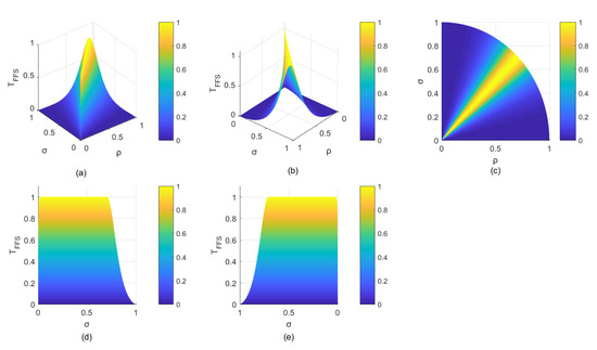
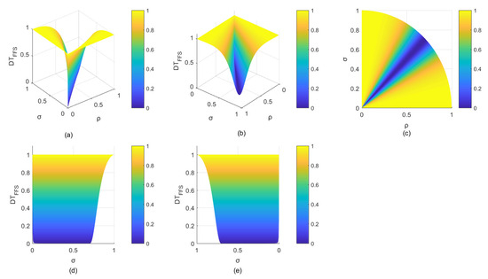
Within the set Z, two FFSs and are identified, characterized by and , respectively. In the present example, the membership and non-membership degrees of and are alternatively denoted by variables ρ and σ, respectively. The variables ρ and σ fall within the interval , and these parameters satisfy condition . The similarity and distance between and are measured by Equations (21) and (26), respectively. Figure 1 and Figure 2 illustrate the trends of similarity and distance between and as the parameters ρ and σ vary within a range of values, respectively.

Figure 1.
Tanimoto similarity measure between and . (a) ; (b) Opposite side of ; (c) Variations of and ; (d) Variations of and ; (e) Variations of and .

Figure 2.
Tanimoto distance measure between and . (a) ; (b) Opposite side of ; (c) Variations of and ; (d) Variations of and ; (e) Variations of and .
According to Figure 1 and Figure 2, the similarity and distance values fall within the interval [0,1]. Notably, when ρ equals σ, the similarity measure between and attains its maximum value of 1. Conversely, when ρ is set to 1 while σ is zero (or vice versa), the similarity measure reaches its minimum value of 0. As parameters ρ and σ vary within the range of [0, 1], the corresponding similarity measure undergoes alterations within the identical interval [0, 1]. The change in distance measure is reversed. These results affirm that the Tanimoto similarity measures and the distance measures satisfy the boundedness Property (1) as stipulated in Definition 11 and Definition 15, respectively. The general direction shown in Figure 1 and Figure 2 is consistent with instinctive reasoning, indicating that the Tanimoto measures adhere to the requirements of Property (1) in Definition 11 and Definition 15.
Example 3.


In the present study, two FFSs, labeled as F and G, under various are examined, as detailed in Table 5. It is evident that the F values for 1 and 2 are identical, whereas the G values differ significantly. Consequently, the similarity measure for 1 is anticipated to be distinct from that of 2. Similarly, the similarity measures for 3, 4, 5, and 6 are also expected to exhibit distinct values from one another. The outcomes of employing diverse similarity measures are presented in Table 6.

Table 5.
FFSs F and G under different Cases.

Table 6.
The outcomes using different similarity measures. The counter-intuitive results in 1 and 2 are highlighted in red, the counter-intuitive results in 3 and 4 are highlighted in blue, and the counter-intuitive results in 5 and 6 are highlighted in green.
The findings reveal that counter-intuitive outcomes are consistently observed in each pair of . For instance, as previously mentioned, under reasonable assumptions, the for 1 would not be equal to that of 2; however, the same values(0.778) are obtained using . It is noteworthy that the majority of similarity measures yield counter-intuitive results. Specifically, , , , and produced counter-intuitive outcomes in Case 1 and Case 2; , and produced counter-intuitive outcomes in Case 3 and Case 4; and , , and produced counter-intuitive outcomes in Case 5 and Case 6. However, the introduced Tanimoto similarity measures exhibit high precision across all scenarios, demonstrating the superiority of our measures.
Example 4.


There are three FFSs in , denoted as and , and presented in Table 7. The data in Table 7 clearly indicate that , implying that the distance between F and , and the similarity between F and , must be distinct. In Table 8, the outcomes of the Tanimoto distance measures and those of the Hellinger distance measure and the triangular distance measure proposed by Deng [69] (indicated as and ) are compared. Obviously, the Tanimoto distance measures offer precise results that correspond well with expectations. Nevertheless, the other distance measures yield results that are at odds with intuition and may not effectively differentiate both FFSs correctly in practice. It can be concluded from this example that our proposed measures enhance accuracy and demonstrate superior performance compared to the Hellinger distance measure and the triangular distance measure.

Table 7.
FFSs F, and .

Table 8.
The outcomes using different distance measures. The counter-intuitive results are highlighted in red.
Example 5.
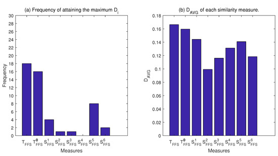
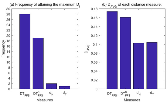
, and are three randomly generated FFSs under case . The current study employs the proposed similarity measures to quantify the resemblance between the two entities, subsequently calculating the discrepancy by taking the difference between the maximum and minimum values derived from these assessments, denoted as . We conducted 50 such experiments and averaged the final results to obtain the average difference between the minimum and maximum values of the similarity results in these 50 experiments, denoted as . Specifically, the and for FFSs can be calculated as follow:
Similarly, we compare the s and s obtained using other measures. Figure 3a presents the frequency of different similarity measures attaining the maximum in these 50 experiments, while Figure 3b depicts the s of different similarity measures across these 50 experiments. We conducted the same experiment using distance measures and the results are presented in Figure 4.

Figure 3.
Differences in results obtained from each similarity measure.

Figure 4.
Differences in results obtained from each distance measures.
Figure 3a illustrates that the Tanimoto similarity measures tend to maximize differences of the similarity between different FFSs while Figure 3b illustrates that the Tanimoto similarity reveals that they produce the maximum average differences between the maximum and minimum similarity values. These findings suggest that our proposed similarity measures generate similarity scores with greater variation, thereby endowing the Tanimoto similarity measures with a greater ability to discern differences across various levels of FFSs. Furthermore, it can exhibit better performance in discriminating FFSs with high similarity. The heightened differences in similarity scores assigned to different FFSs can bolster the trustworthiness of FFSs classification and facilitate more confident decision-making. However, and exhibit the smaller values in Figure 3a,b, indicating a tendency to assign similar values to diverse samples, potentially resulting in greater hesitation when making decisions within the same environment, thereby impeding efficient and confident decision-making. These outcomes underscore the preeminence of our proposed similarity measures over the extant ones under scrutiny. Similarly, we performed the identical analysis on distance measures and achieved the same outcomes, as depicted in Figure 4 corroborating the superiority of our proposed distance measures.
4. Applications
This section presents two models that are designed to tackle pattern recognition, medical diagnosis, and MADM, which are grounded in the suggested measures. To substantiate the efficiency of the models introduced, a series of experiments comparing with the existing measures were conducted.
4.1. A Novel Model for Pattern Recognition and Medical Diagnosis
In the presence of an attribute set , we aim to classify the test samples based on k patterns . Pattern instances are represented by FFSs, indicated as . Similarly, test samples are expressed as FFSs, indicated as . Our goal is to achieve precise classification of the test samples to the provided patterns. The process of recognition is outlined below:
- Step 1
- Compute the Tanimoto similarity(or distance) between and .
- Step 2
- Step 3
- If any pattern has the highest Tanimoto similarity between , then, and belong to the same category:If distance measure is used as the standard of measure, then the following form would be applied:
Example 6


([69]). This example pertains to the pattern recognition of unknown samples, where the domain of discourse consists of their attributes and three known sample categories are represented by FFS . Specifically,
There exists a sample S with unknown category, defined as:
and the proposed Tanimoto measures are employed to classify the unknown sample S into the appropriate category. The recognition process is as delineated below:
- Step 1
- Compute the Tanimoto similarity(or distance) between and S:
- Step 2
- Step 3
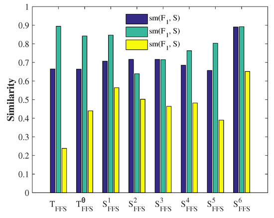
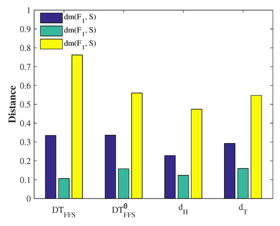
A comparative assessment is conducted with the existing similarity and distance measures mentioned in Section 2. The computational results are presented in Table 9 and Table 10, and the visualized outcomes are displayed in Figure 5 and Figure 6.

Table 9.
The outcomes of different similarity measures.

Table 10.
The outcomes of different distance measures.

Figure 5.
The outcome of different similarity measures.

Figure 6.
The outcomes of different distance measures.
According to the tenet of minimum distance, it was determined that sample S is most similar to sample , which is consistent with the findings in reference [69]. It should be noteworthy that similar recognition results have also been yielded by other distance measures. Furthermore, based on the principle of maximum similarity, similarity measures , , and yielded the same recognition results, classifying sample S into . Conversely, the results of and are different, as they classify sample S as . Therefore, the accuracy of and remains to be discussed. These findings effectively demonstrate the utility of our proposed Tanimoto similarity and distance measures.
Example 7.


This instance is about mineral categories in pattern recognition. Suppose that there are five typical mixed minerals represented by FFS , and each mineral is composed of six basic minerals which form the universe of discourse . Our objective is to use the proposed measures to identify the category to which an unknown mixed mineral S belongs. Table 11 shows the known FFSs and unknown S, while Table 12 and Table 13 summarize the results obtained from similarity and distance measures, respectively.

Table 11.
Known FFSs and a simple S.

Table 12.
The results of different similarity measures.

Table 13.
The results of different distance measures.
Table 12 reveals that the Tanimoto similarity of mineral S and is the highest, suggesting that mineral S belongs to . This is consistent with the results of other similarity measures. In addition, as depicted in Table 13, the Tanimoto distance between mineral S and is minimal, indicating that mineral S is the closest to . These findings align with the results obtained from other distance measures. The results of our experiments provide evidence for the effectiveness of the proposed measures.
Example 8


([77]). There are four individuals afflicted with the following symptoms: Headache, Acidity, Burning eyes, Back pain, and Depression. These patients, identified as Ragu, Mathi, Velu, and Karthi, are collectively referred to as . Their symptoms are encapsulated as . The set of possible diagnoses is denoted by , and includes: : Stress; : Ulcer; : Visual impairment (VI); : Spinal problem (SP); : Blood pressure (BP). The relationship is expressed by FFSs, as presented in Table 14, while the relationship is represented by FFSs and listed in Table 15. Every entry in both tables is determined through the FFS, with the values indicating the degrees of membership and non-membership, respectively. The introduced similarity and distance measures are employed to quantify the similarity and distance between each patient and potential diagnosis. Diagnoses are established for each patient aligning with the principles of maximum similarity or minimum distance. Table 16, Table 17 and Table 18 present the similarity measure outcomes and distance of patient I towards each diagnosis D, alongside the ultimate diagnosis results.

Table 14.
Symptomatic characteristic of the patients.

Table 15.
Symptomatic characteristic of the diagnosis.

Table 16.
Diagnostic results of the Tanimoto similarity measures.

Table 17.
Diagnostic results of the Tanimoto distance measures.

Table 18.
The results of different measures.
Based on the findings presented in Table 16 and Table 17, it is observed that exhibits the highest Tanimoto similarity measure and the smallest Tanimoto distance measure towards ; displays the highest Tanimoto similarity measure and the smallest Tanimoto distance measure towards ; demonstrates the highest Tanimoto similarity measure and the smallest Tanimoto distance measure towards , and showcases the highest Tanimoto similarity measure and the smallest Tanimoto distance measure towards . Thus, we can conclude that Ragu exhibits signs of stress, while Mathi is suffering from spinal issues, Velu is experiencing vision-related difficulties, and Karthi is under stress.
We compared and analyzed the proposed measures with other technologies to verify their effectiveness, and the outcomes have been outlined in Table 18. The information revealed in Table 18 reveals that our suggested measures yield diagnostic outcomes that align with those derived from Ding and Xiao’s method [77] and Deng’s method [69], indicating the potential of our measures to address medical diagnostic challenges. The experimental findings lend support to the viability of our introduced similarity and distance measures. These measures assist healthcare professionals in identifying the diagnosis that best matches the patient’s symptoms, thereby facilitating the formulation of the most appropriate treatment plan. By comparing the similarity between the patient’s symptoms and established diagnoses, a probabilistic diagnosis can be derived, which is particularly useful for cases characterized by atypical symptoms or multiple morbidities.
4.2. A Novel Model for MADM
Consider a discrete collection of options denoted by , along with an attribute set . Let represent the vector of attribute weights for (where ), where , . Consider that is the Fermatean fuzzy matrix, where represents the degree to which alternative fulfills attribute , and represents the degree to which alternative falls short of attribute , , , , , . The proposed model is described below:
- Step 1
- Introducing the Fermatean fuzzy positive ideal solution :When an attribute is a negative influence, we define the positive ideal solution as .
- Step 2
- Computing the weighted Tanimoto similarity measures(or the Tanimoto distance measures) between and through the following formula:or
- Step 3
- Evaluate and order all available options and determine the most preferable choice(s) based on their respective weighted Tanimoto similarity measures or the weighted Tanimoto distance measures. If an alternative exhibits a higher weighted Tanimoto similarity or the smaller weighted Tanimoto distance, it is a more important alternative. If any alternative has the highest weighted Tanimoto similarity value or the smallest Tanimoto distance value, then, it would be considered the most significant alternative.
Example 9.

A certain company intends to procure a set of computers from a pool of five alternative model options, denoted as . The company has identified four crucial attributes for selection, namely, manufacturing materials, response speed, service life, and after-sales quality . These attributes are allocated weights, denoted as ), where , which together form the Fermatean fuzzy decision matrix R:
We advocate for the application of the MADM model to identify the most suitable solution.
- Step 1
- Introducing the Fermatean fuzzy positive ideal solution :Here, all attributes are considered positive attributes, so they are defined as (1, 0)
- Step 2
 Table 19. The computational results derived from the Tanimoto similarity measures.
 Table 20. The computational results derived from the Tanimoto distance measures.
- Step 3
- For ease of observation, the results are presented as Figure 7 and Figure 8. We can find that the weighted similarity between and achieves its maximum level, similarly, the weighted distance between and is at its minimum, so we choose the best alternative.
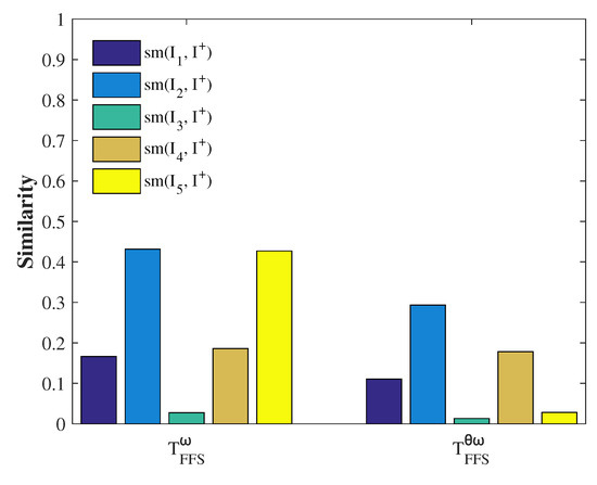 Figure 7. The computational results derived from the Tanimoto similarity measures.
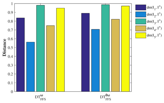 Figure 8. The computational results derived from the Tanimoto distance measures.
Furthermore, we obtained the same selection result using the TOPSIS method proposed by Murat [70], and the calculation outcomes are presented in Table 21. The closeness index γ and the positive ideal solution proposed by Murat are utilized in this study. As the γ gets smaller, is taken as the best alternative.

Table 21.
The results of Murat.
Example 10.
At present, there are five students available, from whom a certain company needs to select two interns. A suite of selection criteria has been developed, which considers the student’s academic performance, competition participation, school activities, mastery of professional knowledge related to the position and violations of discipline on campus. However, violations of discipline on campus are not considered positive attributes. Weights have been assigned to each attribute, resulting in the formation of a Fermatean fuzzy decision matrix R:
The proposed MADM model is being utilized for selecting the most suitable interns:
- Step 1
- Introducing the Fermatean fuzzy positive ideal solution :Here, campus disciplinary behavior is not considered a positive factor and is therefore defined as (0, 1).
- Step 2
 Table 22. The results of Tanimoto similarity measures.
 Table 23. The results of Tanimoto distance measures.
- Step 3
- Table 24 presents the sorted similarity measures and distance measures based on the obtained data, in accordance with the principles of maximum similarity and minimum distance. Adhering to the principles of maximum similarity and minimum distance, we choose and as the optimal choices.
 Table 24. Ranking of Tanimoto measures results.
5. Conclusions
Fermatean fuzzy sets (FFSs) are an effective tool for representing uncertain information. However, the accurate measure of similarity and distance between two FFSs remains a long-term research issue. In the present investigation, we present a suite of novel similarity and distance measures for FFSs, drawing upon the Tanimoto measure. Computational experiments validate that our proposed measures circumvent the counter-intuitive outcomes prevalent in many current measures while offering more discernible differentiation when distinguishing FFSs. Our measures exhibit enhanced efficacy and superiority when contrasted with certain existing FFSs measures. Furthermore, we utilized our measures in the context of pattern recognition, medical diagnostics, and multi-attribute decision-making within Fermatean fuzzy settings, yielding outcomes that are both effective and rational. Consequently, our methods are adeptly suited for assessing feature similarity and facilitating decision-making in intricate and uncertain situations. Moving forward, we intend to explore synergies with a variety of complementary methodologies, such as learning operators with coupled attention [78], the extension of the COPRAS method [79], complex cubic q-rung ortho-pair fuzzy sets [80], minimum weight optimization [81], Frank aggregation operators [82], and IVq-ROF weighted geometric operators [83]. We aim to apply these integrated approaches to address uncertainty within image segmentation, object recognition, and image classification tasks, as well as to tackle data analysis challenges in clustering, classification, and regression. By leveraging these advanced techniques, we aspire to enhance the robustness and accuracy of our methodologies in managing the intricacies of uncertainty across these diverse application domains.
Author Contributions
Conceptualization, H.W.; Methodology, H.W.; Visualization, H.W.; Software, Z.W.; Investigation, Z.W.; Data curation, C.T.; Writing—original draft, H.W.; Writing—review & editing, C.L.; Project administration, C.L.; Funding acquisition, C.L. and G.F. All authors have read and agreed to the published version of the manuscript.
Funding
This research was funded by National Natural Science Foundation of China grant number 62102235 and Natural Science Foundation of Shandong Province grant number ZR2020QF029.
Data Availability Statement
Both data and algorithms are listed in the article.
Conflicts of Interest
The authors declare no conflicts of interest.
References
- Yager, R.R. On using the Shapley value to approximate the Choquet integral in cases of uncertain arguments. IEEE Trans. Fuzzy Syst. 2017, 26, 1303–1310. [Google Scholar] [CrossRef]
- Wang, X.; Song, Y. Uncertainty measure in evidence theory with its applications. Appl. Intell. 2018, 48, 1672–1688. [Google Scholar] [CrossRef]
- Hariri, R.H.; Fredericks, E.M.; Bowers, K.M. Uncertainty in big data analytics: Survey, opportunities, and challenges. J. Big Data 2019, 6, 44. [Google Scholar] [CrossRef]
- Zadeh, L.A. Fuzzy sets. Inf. Control 1965, 8, 338–353. [Google Scholar] [CrossRef]
- Zadeh, L.A. Fuzzy sets as a basis for a theory of possibility. Fuzzy Sets Syst. 1978, 1, 3–28. [Google Scholar] [CrossRef]
- Torra, V. Hesitant fuzzy sets. Int. J. Intell. Syst. 2010, 25, 529–539. [Google Scholar] [CrossRef]
- Hung, W.L.; Yang, M.S. Fuzzy entropy on intuitionistic fuzzy sets. Int. J. Intell. Syst. 2010, 21, 443–451. [Google Scholar] [CrossRef]
- Pawlak, Z. Rough sets. Int. J. Comput. Inf. Sci. 1982, 11, 341–356. [Google Scholar] [CrossRef]
- Deng, Y. Uncertainty measure in evidence theory. Sci. China Inf. Sci. 2020, 63, 210201. [Google Scholar] [CrossRef]
- Kabir, S.; Papadopoulos, Y. A review of applications of fuzzy sets to safety and reliability engineering. Int. J. Approx. Reason. 2018, 100, 29–55. [Google Scholar] [CrossRef]
- Thong, N.T.; Son, L.H. HIFCF: An effective hybrid model between picture fuzzy clustering and intuitionistic fuzzy recommender systems for medical diagnosis. Expert Syst. Appl. 2015, 42, 3682–3701. [Google Scholar] [CrossRef]
- Haseli, G.; Sheikh, R.; Wang, J.; Tomaskova, H.; Tirkolaee, E.B. A novel approach for group decision making based on the best–worst method (G-bwm): Application to supply chain management. Mathematics 2021, 9, 1881. [Google Scholar] [CrossRef]
- Ma, Z.; Liu, Z.; Luo, C.; Song, L. Evidential classification of incomplete instance based on K-nearest centroid neighbor. J. Intell. Fuzzy Syst. 2021, 41, 7101–7115. [Google Scholar] [CrossRef]
- Mardani, A.; Hooker, R.E.; Ozkul, S.; Yifan, S.; Nilashi, M.; Sabzi, H.Z.; Fei, G.C. Application of decision making and fuzzy sets theory to evaluate the healthcare and medical problems: A review of three decades of research with recent developments. Expert Syst. Appl. 2019, 137, 202–231. [Google Scholar] [CrossRef]
- Hwang, G.J.; Tu, Y.F. Roles and research trends of artificial intelligence in mathematics education: A bibliometric mapping analysis and systematic review. Mathematics 2021, 9, 584. [Google Scholar] [CrossRef]
- Atanassov, K.T. Intuitionistic fuzzy sets. Fuzzy Sets Syst. 1986, 20, 87–96. [Google Scholar] [CrossRef]
- Shafer, G. A Mathematical Theory of Evidence; Princeton University Press: Princeton, NJ, USA, 1976; Volume 42. [Google Scholar]
- Wang, G. Rough reduction in algebra view and information view. Int. J. Intell. Syst. 2003, 18, 679–688. [Google Scholar] [CrossRef]
- Alcantud, J.C.R.; Khameneh, A.Z.; Kilicman, A. Aggregation of infinite chains of intuitionistic fuzzy sets and their application to choices with temporal intuitionistic fuzzy information. Inf. Sci. 2020, 514, 106–117. [Google Scholar] [CrossRef]
- Balasubramaniam, P.; Ananthi, V. Image fusion using intuitionistic fuzzy sets. Inf. Fusion 2014, 20, 21–30. [Google Scholar] [CrossRef]
- Ngan, R.T.; Ali, M.; Fujita, H.; Abdel-Basset, M.; Giang, N.L.; Manogaran, G.; Priyan, M. A new representation of intuitionistic fuzzy systems and their applications in critical decision making. IEEE Intell. Syst. 2019, 35, 6–17. [Google Scholar]
- Yager, R.R. Pythagorean fuzzy subsets. In Proceedings of the 2013 Joint IFSA World Congress and NAFIPS Annual Meeting (IFSA/NAFIPS), Edmonton, AB, Canada, 24–28 June 2013; IEEE: Piscataway, NJ, USA, 2013; pp. 57–61. [Google Scholar]
- Premalatha, R.; Dhanalakshmi, P. Enhancement and segmentation of medical images through Pythagorean fuzzy sets—An innovative approach. Neural Comput. Appl. 2022, 34, 11553–11569. [Google Scholar] [CrossRef]
- Naeem, K.; Riaz, M.; Karaaslan, F. Some novel features of Pythagorean m-polar fuzzy sets with applications. Complex Intell. Syst. 2021, 7, 459–475. [Google Scholar] [CrossRef]
- Li, L.; Zhang, R.; Wang, J.; Zhu, X.; Xing, Y. Pythagorean fuzzy power Muirhead mean operators with their application to multi-attribute decision making. J. Intell. Fuzzy Syst. 2018, 35, 2035–2050. [Google Scholar] [CrossRef]
- Ali, G.; Ansari, M.N. Multiattribute decision-making under Fermatean fuzzy bipolar soft framework. Granul. Comput. 2022, 7, 337–352. [Google Scholar] [CrossRef]
- Senapati, T.; Yager, R.R. Fermatean fuzzy sets. J. Ambient. Intell. Humaniz. Comput. 2019, 11, 663–674. [Google Scholar] [CrossRef]
- Kirisci, M. Correlation coefficients of fermatean fuzzy sets with a medical application. J. Math. Sci. Model. 2022, 5, 16–23. [Google Scholar]
- Ejegwa, P.; Muhiuddin, G.; Algehyne, E.; Agbetayo, J.; Al-Kadi, D. An Enhanced Fermatean Fuzzy Composition Relation Based on a Maximum-Average Approach and Its Application in Diagnostic Analysis. J. Math. 2022, 2022, 1786221. [Google Scholar] [CrossRef]
- Chang, K.H.; Chung, H.Y.; Wang, C.N.; Lai, Y.D.; Wu, C.H. A new hybrid Fermatean fuzzy set and entropy method for risk assessment. Axioms 2023, 12, 58. [Google Scholar] [CrossRef]
- Akram, M.; Shahzadi, G.; Davvaz, B. Decision-making model for internet finance soft power and sportswear brands based on sine-trigonometric Fermatean fuzzy information. Soft Comput. 2023, 27, 1971–1983. [Google Scholar] [CrossRef]
- Keshavarz-Ghorabaee, M.; Amiri, M.; Hashemi-Tabatabaei, M.; Zavadskas, E.K.; Kaklauskas, A. A new decision-making approach based on Fermatean fuzzy sets and WASPAS for green construction supplier evaluation. Mathematics 2020, 8, 2202. [Google Scholar] [CrossRef]
- Garg, H.; Shahzadi, G.; Akram, M. Decision-making analysis based on Fermatean fuzzy Yager aggregation operators with application in COVID-19 testing facility. Math. Probl. Eng. 2020, 2020, 7279027. [Google Scholar] [CrossRef]
- Aydemir, S.B.; Yilmaz Gunduz, S. Fermatean fuzzy TOPSIS method with Dombi aggregation operators and its application in multi-criteria decision making. J. Intell. Fuzzy Syst. 2020, 39, 851–869. [Google Scholar] [CrossRef]
- Shahzadi, G.; Akram, M. Group decision-making for the selection of an antivirus mask under fermatean fuzzy soft information. J. Intell. Fuzzy Syst. 2021, 40, 1401–1416. [Google Scholar] [CrossRef]
- Gul, M.; Lo, H.W.; Yucesan, M. Fermatean fuzzy TOPSIS-based approach for occupational risk assessment in manufacturing. Complex Intell. Syst. 2021, 7, 2635–2653. [Google Scholar] [CrossRef]
- Sergi, D.; Sari, I.U. Fuzzy capital budgeting using fermatean fuzzy sets. In Intelligent and Fuzzy Techniques: Smart and Innovative Solutions, Proceedings of the INFUS 2020 Conference, Istanbul, Turkey, 21–23 July 2020; Springer: Cham, Switzerland, 2021; pp. 448–456. [Google Scholar]
- Sivadas, A.; John, S.J. Fermatean Fuzzy Soft Sets and Its Applications; Springer: Singapore, 2021; pp. 203–216. [Google Scholar]
- Xu, C.; Shen, J. Multi-criteria decision making and pattern recognition based on similarity measures for Fermatean fuzzy sets. J. Intell. Fuzzy Syst. 2021, 41, 5847–5863. [Google Scholar] [CrossRef]
- Zeng, L.; Ren, H.; Yang, T.; Xiong, N. An Intelligent Expert Combination Weighting Scheme for Group Decision Making in Railway Reconstruction. Mathematics 2022, 10, 549. [Google Scholar] [CrossRef]
- Akram, M.; Shah, S.M.U.; Al-Shamiri, M.M.A.; Edalatpanah, S. Fractional transportation problem under interval-valued Fermatean fuzzy sets. AIMS Math. 2022, 7, 17327–17348. [Google Scholar] [CrossRef]
- Ye, J. Cosine similarity measures for intuitionistic fuzzy sets and their applications. Math. Comput. Model. 2011, 53, 91–97. [Google Scholar] [CrossRef]
- Salton, G. Introduction to Modern Information Retrieval; McGraw-Hill: New York, NY, USA, 1983. [Google Scholar]
- Garg, H.; Rani, D. Novel similarity measure based on the transformed right-angled triangles between intuitionistic fuzzy sets and its applications. Cogn. Comput. 2021, 13, 447–465. [Google Scholar] [CrossRef]
- Huang, J.; Jin, X.; Lee, S.J.; Huang, S.; Jiang, Q. An effective similarity/distance measure between intuitionistic fuzzy sets based on the areas of transformed isosceles right triangle and its applications. J. Intell. Fuzzy Syst. 2021, 40, 9289–9309. [Google Scholar] [CrossRef]
- Olgun, M.; Türkarslan, E.; Ünver, M.; Ye, J. A cosine similarity measure based on the Choquet integral for intuitionistic fuzzy sets and its applications to pattern recognition. Informatica 2021, 32, 849–864. [Google Scholar] [CrossRef]
- Kumar, R.; Kumar, S. A novel intuitionistic fuzzy similarity measure with applications in decision-making, pattern recognition, and clustering problems. Granul. Comput. 2023, 7, 1027–1050. [Google Scholar] [CrossRef]
- Duan, J.; Li, X. Similarity of intuitionistic fuzzy sets and its applications. Int. J. Approx. Reason. 2021, 137, 166–180. [Google Scholar] [CrossRef]
- Garg, H. A novel correlation coefficients between Pythagorean fuzzy sets and its applications to decision-making processes. Int. J. Intell. Syst. 2016, 31, 1234–1252. [Google Scholar] [CrossRef]
- Li, J.; Wen, L.; Wei, G.; Wu, J.; Wei, C. New similarity and distance measures of Pythagorean fuzzy sets and its application to selection of advertising platforms. J. Intell. Fuzzy Syst. 2021, 40, 5403–5419. [Google Scholar] [CrossRef]
- Hussian, Z.; Yang, M.S. Distance and similarity measures of Pythagorean fuzzy sets based on the Hausdorff metric with application to fuzzy TOPSIS. Int. J. Intell. Syst. 2019, 34, 2633–2654. [Google Scholar] [CrossRef]
- Mahmood, T.; Ur Rehman, U.; Ali, Z.; Mahmood, T. Hybrid vector similarity measures based on complex hesitant fuzzy sets and their applications to pattern recognition and medical diagnosis. J. Intell. Fuzzy Syst. 2021, 40, 625–646. [Google Scholar] [CrossRef]
- Thao, N.X.; Chou, S.Y. Novel similarity measures, entropy of intuitionistic fuzzy sets and their application in software quality evaluation. Soft Comput. 2022, 53, 2009–2020. [Google Scholar] [CrossRef]
- Farhadinia, B. Similarity-based multi-criteria decision making technique of pythagorean fuzzy sets. Artif. Intell. Rev. 2022, 55, 2103–2148. [Google Scholar] [CrossRef]
- Ilieva, G.; Yankova, T. Extension of interval-valued Fermatean fuzzy TOPSIS for evaluating and benchmarking COVID-19 vaccines. Mathematics 2022, 10, 3514. [Google Scholar] [CrossRef]
- Albaity, M.; Mahmood, T. Medical diagnosis and pattern recognition based on generalized dice similarity measures for managing intuitionistic hesitant fuzzy information. Mathematics 2022, 10, 2815. [Google Scholar] [CrossRef]
- Naeem, M.; Qiyas, M.; Al-Shomrani, M.M.; Abdullah, S. Similarity measures for fractional orthotriple fuzzy sets using cosine and cotangent functions and their application in accident emergency response. Mathematics 2020, 8, 1653. [Google Scholar] [CrossRef]
- Li, R.; Zhang, H.; Zhang, X.; Wu, Q. A similarity measure based on fuzzy entropy for image segmentation. Entropy 2019, 21, 610. [Google Scholar]
- Grzegorzewski, P. Distances between intuitionistic fuzzy sets and/or interval-valued fuzzy sets based on the Hausdorff metric. Fuzzy Sets Syst. 2004, 148, 319–328. [Google Scholar] [CrossRef]
- Gohain, B.; Dutta, P.; Gogoi, S.; Chutia, R. Construction and generation of distance and similarity measures for intuitionistic fuzzy sets and various applications. Int. J. Intell. Syst. 2021, 36, 7805–7838. [Google Scholar] [CrossRef]
- Mahanta, J.; Panda, S. A novel distance measure for intuitionistic fuzzy sets with diverse applications. Int. J. Intell. Syst. 2021, 36, 615–627. [Google Scholar] [CrossRef]
- Xiao, F. A distance measure for intuitionistic fuzzy sets and its application to pattern classification problems. IEEE Trans. Syst. Man Cybern. Syst. 2019, 51, 3980–3992. [Google Scholar] [CrossRef]
- Li, D.; Zeng, W. Distance measure of Pythagorean fuzzy sets. Int. J. Intell. Syst. 2018, 33, 348–361. [Google Scholar] [CrossRef]
- Zeng, W.; Cui, H.; Liu, Y.; Yin, Q.; Xu, Z. Novel distance measure between intuitionistic fuzzy sets and its application in pattern recognition. Iran. J. Fuzzy Syst. 2022, 19, 127–137. [Google Scholar]
- Talebi, S.P.; Godsill, S.J.; Mandic, D.P. Filtering structures for α-stable systems. IEEE Control Syst. Lett. 2022, 7, 553–558. [Google Scholar] [CrossRef]
- Li, Z.; Lu, M. Some novel similarity and distance measures of pythagorean fuzzy sets and their applications. J. Intell. Fuzzy Syst. 2019, 37, 1781–1799. [Google Scholar] [CrossRef]
- Zhang, X.; Xu, Z. Extension of TOPSIS to multiple criteria decision making with Pythagorean fuzzy sets. Int. J. Intell. Syst. 2014, 29, 1061–1078. [Google Scholar] [CrossRef]
- Ren, P.; Xu, Z.; Gou, X. Pythagorean fuzzy TODIM approach to multi-criteria decision making. Appl. Soft Comput. 2016, 42, 246–259. [Google Scholar] [CrossRef]
- Deng, Z.; Wang, J. New distance measure for Fermatean fuzzy sets and its application. Int. J. Intell. Syst. 2022, 37, 1903–1930. [Google Scholar] [CrossRef]
- Kirişci, M. New cosine similarity and distance measures for Fermatean fuzzy sets and TOPSIS approach. Knowl. Inf. Syst. 2023, 65, 855–868. [Google Scholar] [CrossRef] [PubMed]
- Sahoo, L. Similarity measures for Fermatean fuzzy sets and its applications in group decision-making. Decis. Sci. Lett. 2022, 11, 167–180. [Google Scholar] [CrossRef]
- Liu, D.; Liu, Y.; Wang, L. Distance measure for Fermatean fuzzy linguistic term sets based on linguistic scale function: An illustration of the TODIM and TOPSIS methods. Int. J. Intell. Syst. 2019, 34, 2807–2834. [Google Scholar] [CrossRef]
- Lipkus, A.H. A proof of the triangle inequality for the Tanimoto distance. J. Math. Chem. 1999, 26, 263–265. [Google Scholar] [CrossRef]
- Wikipedia Contributors. Jaccard Index—Wikipedia. The Free Encyclopedia. 2024. Available online: https://en.wikipedia.org/w/index.php?title=Jaccard_index&oldid=1196092673 (accessed on 16 January 2024).
- Bajusz, D.; Rácz, A.; Héberger, K. Why is Tanimoto index an appropriate choice for fingerprint-based similarity calculations? J. Cheminform. 2015, 7, 20. [Google Scholar] [CrossRef]
- Chung, N.C.; Miasojedow, B.; Startek, M.; Gambin, A. Jaccard/Tanimoto similarity test and estimation methods for biological presence-absence data. BMC Bioinform. 2019, 20, 644. [Google Scholar] [CrossRef]
- Xiao, F.; Ding, W. Divergence measure of Pythagorean fuzzy sets and its application in medical diagnosis. Appl. Soft Comput. 2019, 79, 254–267. [Google Scholar] [CrossRef]
- Kissas, G.; Seidman, J.H.; Guilhoto, L.F.; Preciado, V.M.; Pappas, G.J.; Perdikaris, P. Learning operators with coupled attention. J. Mach. Learn. Res. 2022, 23, 9636–9698. [Google Scholar]
- Akram, M.; Ramzan, N.; Feng, F. Extending COPRAS method with linguistic Fermatean fuzzy sets and Hamy mean operators. J. Math. 2022, 2022, 8239263. [Google Scholar] [CrossRef]
- Yu, Q. Hamacher Operations for Complex Cubic q-Rung Orthopair Fuzzy Sets and Their Application to Multiple-Attribute Group Decision Making. Symmetry 2023, 15, 2118. [Google Scholar] [CrossRef]
- Farid, M.; Lim, H.S.; Lee, C.P.; Latip, R. Scheduling Scientific Workflow in Multi-Cloud: A Multi-Objective Minimum Weight Optimization Decision-Making Approach. Symmetry 2023, 15, 2047. [Google Scholar] [CrossRef]
- Yang, X.; Mahmood, T.; Ali, Z.; Hayat, K. Identification and Classification of Multi-Attribute Decision-Making Based on Complex Intuitionistic Fuzzy Frank Aggregation Operators. Mathematics 2023, 11, 3292. [Google Scholar] [CrossRef]
- Yang, X.; Hayat, K.; Raja, M.S.; Yaqoob, N.; Jana, C. Aggregation and interaction aggregation soft operators on interval-valued q-rung orthopair fuzzy soft environment and application in automation company evaluation. IEEE Access 2022, 10, 91424–91444. [Google Scholar] [CrossRef]
Disclaimer/Publisher’s Note: The statements, opinions and data contained in all publications are solely those of the individual author(s) and contributor(s) and not of MDPI and/or the editor(s). MDPI and/or the editor(s) disclaim responsibility for any injury to people or property resulting from any ideas, methods, instructions or products referred to in the content. |
© 2024 by the authors. Licensee MDPI, Basel, Switzerland. This article is an open access article distributed under the terms and conditions of the Creative Commons Attribution (CC BY) license (https://creativecommons.org/licenses/by/4.0/).