Article

Semi-Symmetrical, Fully Convolutional Masked Autoencoder for TBM Muck Image Segmentation

Key Laboratory of Urban Underground Engineering of Ministry of Education, Beijing Jiaotong University, Beijing 100044, China
*
Author to whom correspondence should be addressed.
Symmetry 2024, 16(2), 222; https://doi.org/10.3390/sym16020222
Submission received: 18 January 2024 / Revised: 4 February 2024 / Accepted: 9 February 2024 / Published: 12 February 2024
(This article belongs to the Special Issue Symmetry Applied in Computer Vision, Automation, and Robotics)

Abstract

:
Deep neural networks are effectively utilized for the instance segmentation of muck images from tunnel boring machines (TBMs), providing real-time insights into the surrounding rock condition. However, the high cost of obtaining quality labeled data limits the widespread application of this method. Addressing this challenge, this study presents a semi-symmetrical, fully convolutional masked autoencoder designed for self-supervised pre-training on extensive unlabeled muck image datasets. The model features a four-tier sparse encoder for down-sampling and a two-tier sparse decoder for up-sampling, connected via a conventional convolutional neck, forming a semi-symmetrical structure. This design enhances the model’s ability to capture essential low-level features, including geometric shapes and object boundaries. Additionally, to circumvent the trivial solutions in pixel regression that the original masked autoencoder faced, Histogram of Oriented Gradients (HOG) descriptors and Laplacian features have been integrated as novel self-supervision targets. Testing shows that the proposed model can effectively discern essential features of muck images in self-supervised training. When applied to subsequent end-to-end training tasks, it enhances the model’s performance, increasing the prediction accuracy of Intersection over Union (IoU) for muck boundaries and regions by 5.9% and 2.4%, respectively, outperforming the enhancements made by the original masked autoencoder.

1. Introduction

Tunnel boring machines (TBMs) are essential in modern tunnel engineering, appreciated for their seamless construction process, outstanding boring efficiency, and relatively safe working conditions. Nonetheless, TBMs encounter several challenges in practical applications. Firstly, the efficiency and stability of TBM operations can be greatly compromised in the presence of complex and unpredictable surrounding rock. Secondly, the high integration level of TBM processes necessitates advanced technical skills and experience from operators, where improper handling could not only impair boring efficiency but also risk mechanical failures or accidents. Consequently, many researchers are now turning their attention to the development of automated and intelligent technologies for TBM operations [1,2,3,4,5].
The core idea of TBM intelligent tunneling technology is to collect real-time, multi-faceted information, such as the surrounding rock type, environmental conditions, and mechanical states, during the TBM advancement process. Subsequently, an intelligent decision-making model integrates this information to control the TBM, aiming to achieve efficient, safe, and automated tunnel construction [1]. Among these, the real-time perception technology of the surrounding rock is crucial. Accurate perception of the surrounding rock is a prerequisite for the intelligent decision-making model to produce reasonable results. Due to the requirement for real-time performance, traditional drilling test methods cannot be applied to intelligent tunneling; instead, non-direct detection methods that utilize mediums such as vibration [6], acoustics [7], and electromagnetism [8,9] have become a research focus. In addition, the analysis of muck chip morphology and gradation on the TBM conveyor belt through Computer Vision (CV) technology presents a viable technical route for this real-time perception.
During the TBM excavation process, the cutters induce the fracturing of the rock mass via wedging and squeezing, forming blocky or granular muck. The muck is subsequently transported out of the tunnel using conveyor belts. The morphology of the muck is closely related to the surrounding rock conditions [10,11,12]. Therefore, the characteristics of the surrounding rock can be inferred by capturing images of the muck on the conveyor belts and analyzing its shape, gradation, and other features. The method of analyzing the morphology of geomaterials through image recognition has been widely studied in the past few decades. Early studies typically employed Fourier transforms, Gabor filtering, and wavelet transforms to extract the primary features from digital images of geotechnical materials [13,14]. These were followed by rough estimations of particle size using classification algorithms like Support Vector Machine (SVM). An alternative approach seeks to directly delineate the contours of geotechnical particles by employing traditional image segmentation algorithms, including thresholding and watershed methods [15,16,17]. In recent years, the rapid advancement of deep learning technology has led to methods that use convolutional neural networks (CNNs) or vision transformers (ViTs) for geotechnical material image segmentation, which have achieved results that are far superior to traditional methods [18,19,20,21,22]. However, such neural network models usually require end-to-end training. The major bottleneck is their reliance on a large quantity of high-quality annotated data as training samples. Given the absence of large-scale public datasets, the cost of manually annotating data is prohibitively high, significantly limiting the development of this field.
To address the lack of annotated data, the adoption of self-supervised pre-training coupled with end-to-end fine-tuning presents a viable solution. Self-supervised training involves generating pseudo-labels directly from the input data to guide the learning process, thus allowing the model to train on a substantial volume of unlabeled data. While self-supervised training is well-established in Natural Language Processing (NLP), its progress in CV has been comparatively slow. Initial self-supervised training in CV focused on tasks like denoising and image restoration, employing generative autoencoders to reconstruct missing data from incomplete images and learn their latent features [23,24]. This approach, which involves artificially removing parts of the image information and learning the image features through generative tasks, can be categorized as masked image modeling (MIM) [25,26]. However, in the past decade, another CV self-supervised learning framework—the joint-embedding method, which involves learning features by aligning the embedded representations of augmented views of the same image through a discriminative task—has replaced MIM as the research focus of that time [27,28,29]. Following the success of masked self-supervised training in NLP [30], some studies [31,32] have attempted to adapt this approach to CV tasks, yielding superior results to joint-embedding methods and reviving the prominence of MIM. With the introduction of the masked autoencoder (MAE) [33] and SimMIM [34], the MIM paradigm has evolved and is now widely applied to various downstream tasks [35,36,37], becoming a leading method in CV self-supervised training. This study proposes a self-supervised training method for TBM muck chip segmentation tasks based on the MAE paradigm, aiming to reduce reliance on annotated data, enhance the accuracy of the segmentation model, and further the development of real-time perception of surrounding rock conditions and intelligent excavation technology for TBMs.

1.1. Challenges in TBM Muck Segmentation Task

Muck segmentation presents a highly challenging task. As depicted in Figure 1a, an image of muck chips is captured on the TBM conveyor belt. The rapid movement of muck through the TBM’s conveyor system poses significant challenges for image acquisition. Moreover, the construction site conditions, often compromised by dust and mist, frequently reduce the clarity of captured images. This results in unclear boundaries of the muck chips, complicating their identification. Additionally, as illustrated in Figure 1b (which corresponds to the green frame in Figure 1a), muck chips tend to accumulate naturally, with independent chips often sitting tightly together or overlapping, creating complex textures and structures in the image. These conditions make it difficult for traditional image segmentation algorithms to yield satisfactory results. However, the bodies of muck chips generally possess relatively simple geometric topologies and are limited in size within images (as indicated by the dark yellow frame in Figure 1a), suggesting that muck segmentation requires only low-order semantic features from specific local image areas, without necessitating an overall understanding of the image or long-range dependencies. Furthermore, Figure 1c displays local images within the purple and blue frames from Figure 1a and their rotated counterparts. It can be observed that any local part of the muck image exhibits self-similarity when translated or rotated, indicating that CNN can effectively extract features from muck images.

1.2. Innovation of Our Work

In our current work, we have created a comprehensive dataset of TBM muck images and developed a segmentation algorithm called MuckSeg. This algorithm employs a fully convolutional neural network trained end-to-end, complemented by post-processing algorithms. However, end-to-end training demands a vast quantity of high-quality, annotated data. The segmentation targets in muck images are densely packed; for example, the area depicted in Figure 1d contains 35 muck chips of various sizes and irregular shapes, requiring annotations with more than 500 vertices to delineate their contours—this annotation process is highly labor-intensive. The steep cost of annotation substantially restricts the amount of data available for end-to-end training. Conversely, acquiring unannotated raw muck images is relatively straightforward. Hence, this study introduces a semi-symmetrical, fully convolutional masked autoencoder, named MuckSeg-SS-FCMAE, aiming to improve MuckSeg’s performance. The MuckSeg-SS-FCMAE features two key innovations:
  • The lightweight decoder of the original MAE [33] has been replaced by a multi-tier sparse convolutional decoder. This modification permits the training errors brought forward by the detailed spatial location of low-level features in images to be accurately calculated and back-propagated through the decoder, thus improving the encoder’s feature extraction capabilities.
  • Histogram of Oriented Gradients (HOG) descriptors [38] and labels generated through Gauss–Laplace filtering of the original image—referred to as “Laplacian features” henceforth—have been incorporated as additional self-supervision targets. These enhancements furnish the model with extra training signals for contrast relationships and boundary features, preventing convergence on trivial solutions.
The MuckSeg-SS-FCMAE has been trained on a dataset containing over 40,000 unlabeled muck images. We conducted detailed experiments on its image reconstruction capability, feature extraction ability, and the improvement in instance segmentation task accuracy when transferred to downstream end-to-end training tasks. These experiments demonstrated the effectiveness of the semi-symmetric decoder design and the introduction of additional self-supervision targets for muck segmentation tasks.

1.3. Terms and Abbreviations

For better readability, a summary of the terms and abbreviations used in this article is compiled in Table 1, and they will not be reiterated in the following text.

2. Materials and Methods

2.1. Fundamentals of Fully Convolutional Masked Autoencoders

Masked autoencoders, a variant of masked image modeling methods, exhibit two main characteristics:
  • MAEs obscure a substantial portion (typically over 60%) of the input image on a patch-by-patch basis. A patch is a small, contiguous area within the image, typically measuring 16 × 16 pixels in size. This is the most salient feature distinguishing MAEs from denoising autoencoders. Such masking strategy prevents the model from merely replicating adjacent pixels in the masked areas to reconstruct the image, thereby compelling the model to capture more abstract image features.
  • MAEs generate training signals by comparing the pixel value differences between the model’s output and the original input image. In contrast, BeiT [31] initially pre-trains a dVAE [39] to map image patches to visual tokens and to build a codebook. This process turns the reconstruction of masked areas into a classification task over the codebook. However, experiments using MAEs have demonstrated that the tokenization step is not essential for pre-training in Computer Vision [33].
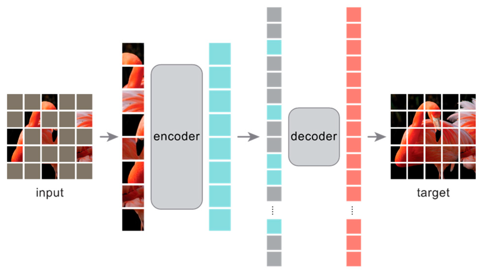
The original MAE structure [33], as depicted in Figure 2, comprises a ViT encoder and a standard transformer decoder. The input image is partitioned into uniform patches of 16 × 16 pixels, and only 25% of these patches are provided to the encoder to derive the masked feature map. A trainable vector, referred to as the ‘mask token’, substitutes the feature maps at the masked locations. Once combined with positional embeddings, these encoder-derived feature maps, along with the mask tokens, are reorganized by position to form a complete feature map that matches the input image’s dimensions. This full feature map is then decoded and reconstructed into an output image that retains the original size and channel count via a linear head.
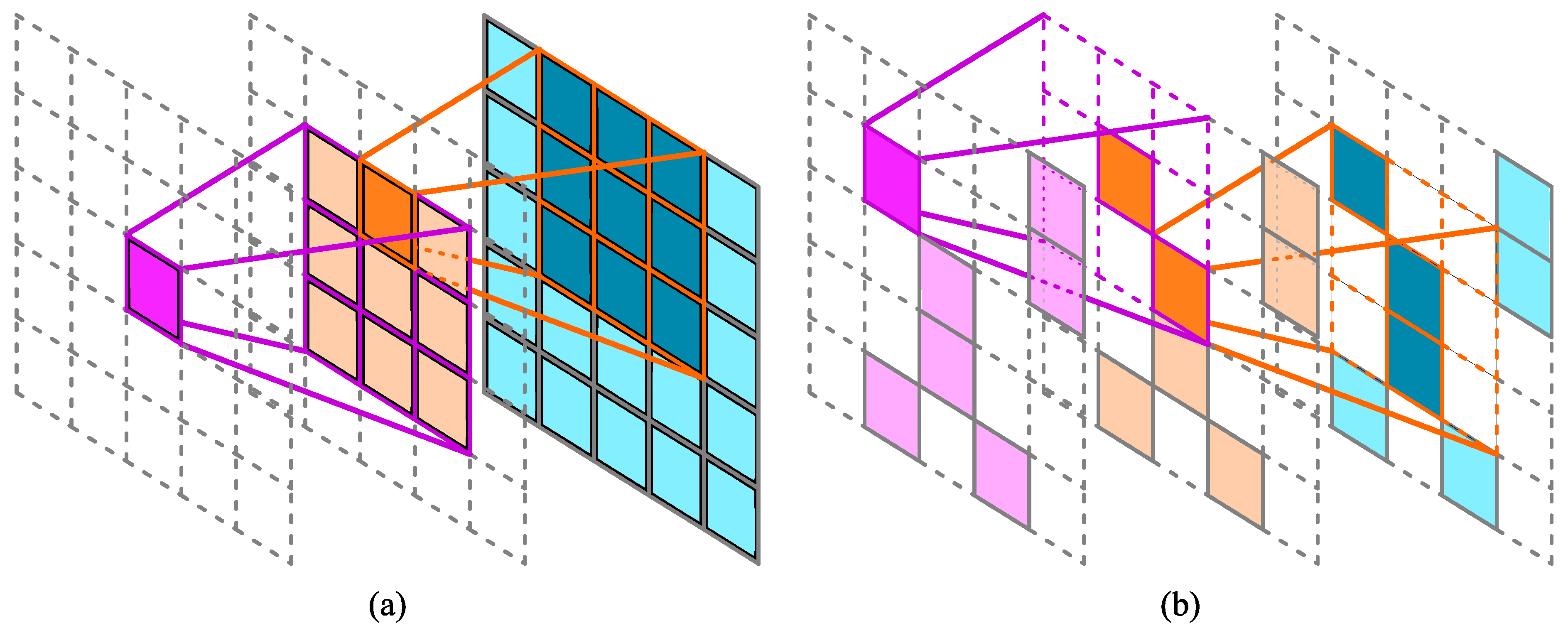
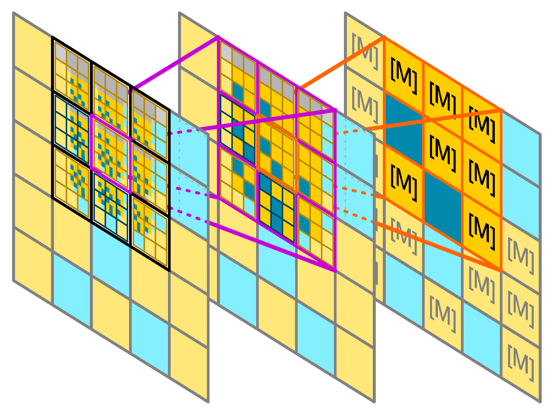
In the original MAE, only the unmasked portions of the input image are fed into the encoder. However, in downstream tasks, the encoder is presented with the entire image. The inherent advantage of the transformer architecture [40]—its ability to process variable-length sequence inputs—makes the implementation of MAE particularly straightforward. However, CNNs must maintain the image’s two-dimensional structure during convolution operations. Masking the input image disrupts this structure, posing challenges to the implementation of a similar process in CNNs. As illustrated in Figure 3a, convolution operations perform weighted summations across all data within the sliding window, traversing every possible spatial position of the input data. This approach is problematic when applied to masked images for two reasons: firstly, the masked sections still contribute to the computational cost despite their calculations being redundant. Secondly, these masked parts, initially zero values, may become non-zero following convolution operations, thus disrupting the masking structure. Repeatedly zeroing out the masked areas after each convolution can mitigate this issue, but it adds computational burden and fails to address the initial shortcoming.
To address this issue, the literature [41] has introduced a fully convolutional version of the MAE that utilizes sparse convolutions [42]. As depicted in Figure 3b, sparse convolution overlooks zero-value pixels at the operator level when an image is represented in a sparse format. As a result, the computation excludes the masked regions of the image, ensuring that the integrity of the masking structure is maintained after the operation. By incorporating sparse convolutions and substituting the transformer block with a ConvNeXt block [41], FCMAE replicates the effects of the original MAE using an entirely CNN-based architecture.

2.2. Design of Semi-Symmetrical, Fully Convolutional Masked Autoencoders

2.2.1. Challenges Associated with the Original MAE in Muck Segmentation Tasks

The original MAE and the SimMIM both utilize an asymmetric architecture, featuring a powerful encoder paired with a lightweight decoder. This configuration emphasizes learning within the encoder during training and ensures the model’s extensive adaptability to diverse downstream tasks, while also curtailing the total parameter count and enhancing training efficiency. Nonetheless, for TBM muck chip image segmentation a lightweight decoder might not be ideal. Muck chip images are predominantly single-channel grayscale, containing sparse high-level semantic content. Instead, crucial information resides in the medium and low-level geometric features, such as the muck chips’ shape, size, and edges. The lightweight decoder attempts to reconstruct the image straight from the high-dimensional feature vectors of individual patches but without the progressive up-sampling present in standard image segmentation decoders, thus it may fail to preserve the essential spatial relationships between pixels in each patch—relationships that are vital for accurate muck segmentation.
On the other hand, the MAE generates a training signal by calculating the pixel-level MSE loss between the reconstructed and original images within the masked region. However, for grayscale images, the pixel-level MSE loss can inadvertently steer the model towards trivial solutions. For instance, Figure 4 displays three 5 × 5 grayscale images, where each grid represents a pixel, with the numbers signifying the pixel values corresponding to their shades of gray. Although Figure 4b seems visually closer to Figure 4a its MSE is surprisingly higher than the MSE between Figure 4b and a uniform gray image (Figure 4c). More problematic is that each of these trivial solutions, like the one shown in Figure 4c, represents a local minima. This issue could lead the model to merely reconstruct basic monochromatic images or textures with clear repetitive patterns, failing to capture finer local nuances.

2.2.2. Self-Supervision Target

To address the aforementioned issue of trivial solution, MuckSeg-SS-FCMAE employs self-supervision objectives that differ from those of the original MAE, which include the following:
  • The input image after 4 × down-sampling.
  • The HOG feature map of the input image. The HOG descriptor, a feature descriptor widely employed in Computer Vision tasks, encapsulates local shape and texture information by calculating the distribution of gradient orientations within localized sections of an image. As depicted in Figure 5, the MuckSeg-SS-FCMAE computes HOG descriptors using 4 × 4 pixel cells across 8 directions. Block normalization is executed over an 8 × 8 pixel block using a 4 × 4 pixel stride, with the L2-Hys normalization method set to a threshold of 0.4. The block-level HOG descriptors are then reorganized into a cell-wise format, as illustrated in Figure 5b. Owing to the potential quadruple utilization of each cell’s HOG descriptor during normalization, this process yields 4 distinct sets of HOG feature vectors with dimensions (W/4) × (H/4) × 8, where W and H represent the width and height of the input image in pixels, respectively. These sets are subsequently concatenated to form a comprehensive HOG feature map with dimensions (W/4) × (H/4) × 32, which serves as the supervision target, as demonstrated in Figure 5c. It is important to note that the HOG feature vectors at the image’s periphery—specifically at the corners and edges—are only employed once or twice in block normalization and are, therefore, replicated to complete the feature map.
  • Boundary features extracted via Gauss–Laplace filtering. The Laplacian filter, a second-order derivative filter, is employed to enhance the edge features in images. Due to its sensitivity to noise, it is typically combined with Gaussian filtering to form Gauss–Laplace filtering. As depicted in Figure 6, the process begins with the input image being blurred with a Gaussian filter with a kernel size of 13. This step is followed by the application of a Laplacian filter with a kernel size of 5, after which the image is normalized. The filtered image is then binarized using a threshold of 0.8, and morphological opening operations are conducted to eliminate noise spots. Finally, the image is down-sampled by a factor of 4 to produce a binary image with dimensions (W/4) × (H/4) × 1, which is used for supervision.

2.2.3. Network Structure

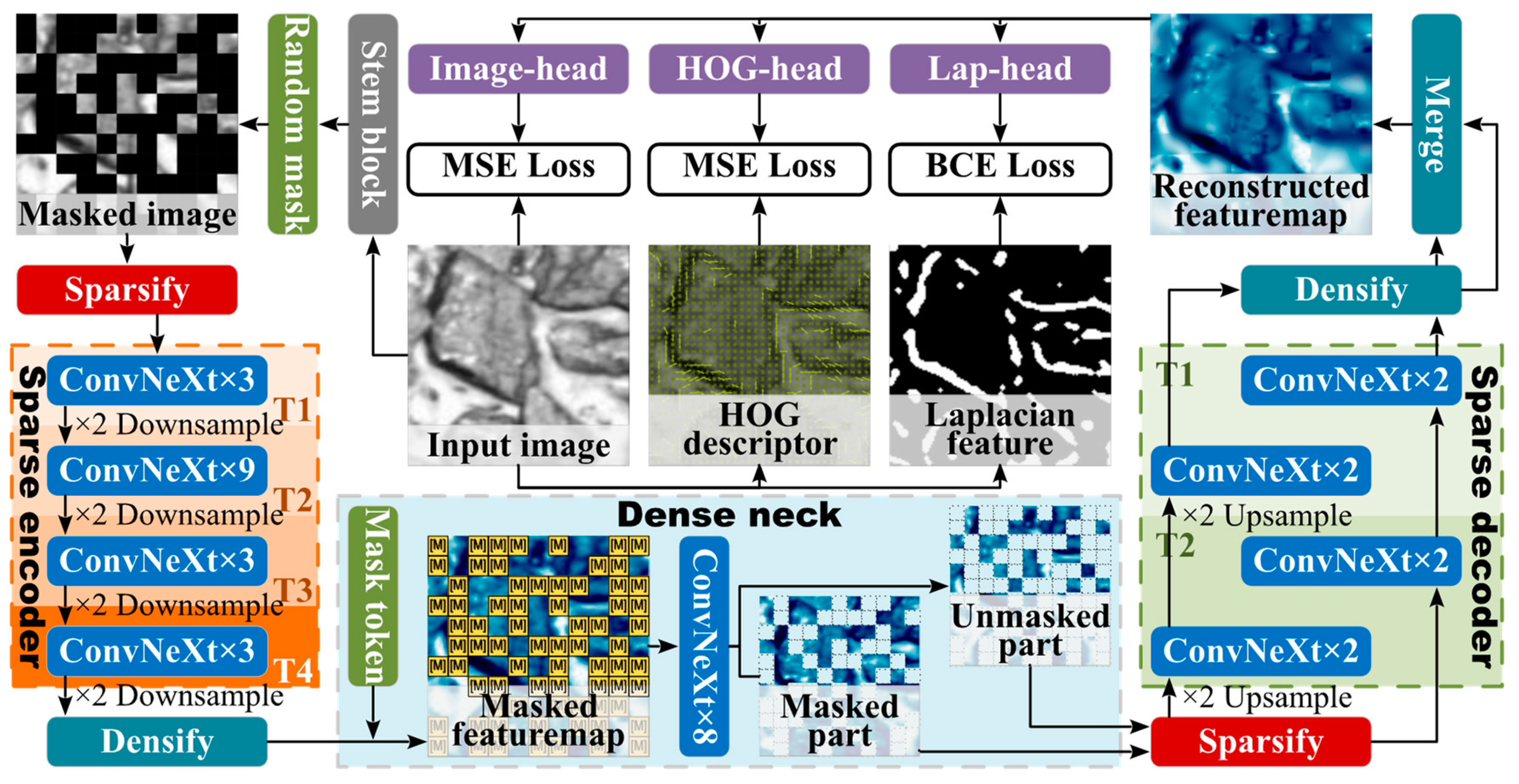
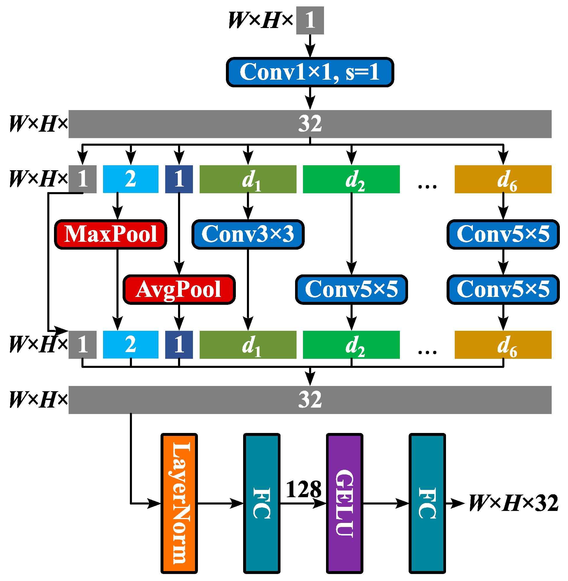
The overall structure of MuckSeg-SS-FCMAE is depicted in Figure 7, comprising a stem block, a sparse encoder, a dense neck, and a sparse decoder. The stem block maps pixel location information from the input image into high-dimensional feature vectors, as detailed in Figure 8. Initially, the image is mapped to a W × H × 32 feature map via a point-wise convolution layer. To reduce feature dimension similarity, the 32-dimensional features are divided into 9 uneven groups, processed by network units (Table 2), and reassembled into a W × H × 32 feature map. These features undergo normalization via LayerNorm and are outputted through an MLP.
Following this, the feature map is segmented into 32 × 32 pixel patches, with roughly 60% randomly masked, converted to a sparse format and input into the encoder. The encoder utilizes a conventional 4-tier pyramidal structure, where each tier comprises several stacked ConvNeXt blocks, a LayerNorm layer, and a convolutional layer with a 2 × 2 kernel size and stride for down-sampling while doubling the feature dimension. The encoder is configured using 3, 9, and 3 ConvNeXt blocks stacked for the 1st, 2nd, and 3rd/4th tiers, respectively. Experimentation revealed that this configuration more effectively extracts features critical for the muck segmentation task. The encoder outputs a 512-dimensional sparse feature map that only contains the unmasked regions, which has been down-sampled by a factor of 16.
Subsequently, the sparse feature map is transformed into a dense representation and compressed into a feature map with the same dimensions as the mask token, which, in our model, is precisely 512. Then, the masked regions within the feature map are substituted with a 512-dimensional mask token. With the encoder’s 16-fold down-sampling, each pixel in this feature map represents a 16 × 16 pixel patch of the original image, with the mask token embodying the semantics of a masked patch. The feature map, now integrated with mask tokens, passes through ConvNeXt blocks in the neck, enabling standard convolution operations and producing a (W/16) × (H/16) × 512 feature map. This process allows masked regions to gain information from unmasked areas. Within the entire MuckSeg-SS-FCMAE framework, the neck serves as the sole gateway for information exchange between masked and unmasked regions, assuming the role of the decoder in the original MAE. To maintain conceptual consistency with the general notion of an encoder–decoder structure, and to differentiate from the encoder and decoder that utilize sparse convolutional operators, this section is referred to as the “dense neck”.
Following the interaction, the feature map is then fed into the decoder. The MuckSeg-SS-FCMAE decoder employs an inverted pyramid design for semantic segmentation, aiming to gradually restore image details by enhancing feature map resolution. However, the decoder features only 2 tiers, with an up-sampling rate of 4, hence this model is termed “semi-symmetrical”. Each tier involves a bilinear up-sampling operation by a factor of 2, two ConvNeXt blocks for feature computation, and a point-wise convolution to reduce feature dimensions. This structure enables the decoder to build a (W/4) × (H/4) × 128 reconstructed feature map from the neck’s (W/16) × (H/16) × 512 output.
To maximize the encoder’s learning, it is crucial to prevent information leakage from unmasked to masked regions in the decoder. As Figure 9 illustrates, using the same convolution kernel for both masked and unmasked regions would cause the information from the unmasked areas (represented in cyan in Figure 9) to gradually spread across the feature map, allowing the decoder to infer masked area information. To avoid this, the decoder employs two independent pipelines. Before each up-sampling operation, the feature map’s masked and unmasked parts are merged in a dense format for up-sampling, and then separated and sparsified again after up-sampling to preventing information leakage.
Lastly, the decoder’s reconstructed feature maps are processed by three parallel convolutional heads, generating predictions for pixel values, HOG descriptors, and Laplacian features. These predictions are compared with self-supervision targets to compute the loss, establishing a complete self-supervised training loop.

2.2.4. Decoder Used for Downstream End-to-End Finetuning

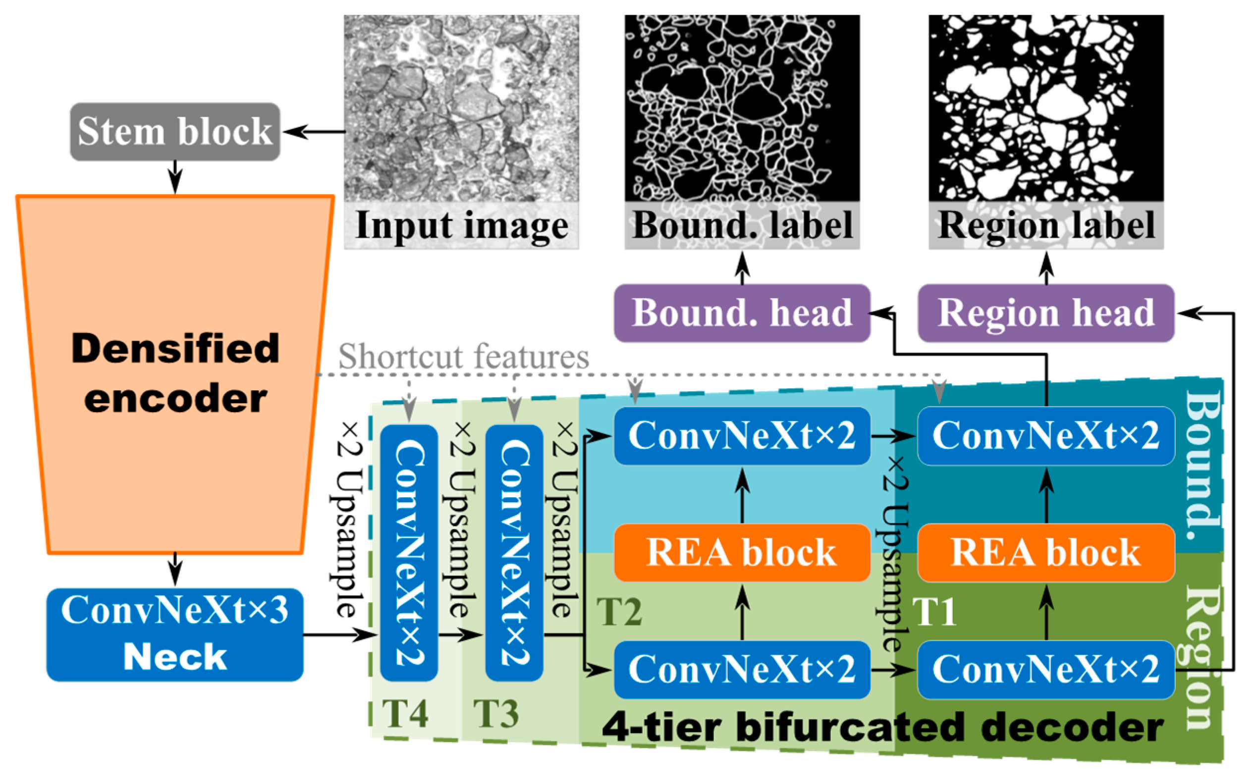
Following MAE training, the stem block and encoder parameters are transferred into the primary MuckSeg network and fine-tuned using labeled data. As depicted in Figure 10, the stem block and encoder of the MuckSeg network are completely identical to those of MuckSeg-SS-FCMAE, but the sparse network layers within the encoder have all been replaced with regular network layers. Following a neck composed of 3 cascaded ConvNeXt blocks is a bifurcated 4-tier decoder that outputs muck boundary and region labels for post-processing.

2.2.5. Loss Function

The training loss for MuckSeg-SS-FCMAE comprises three parts: the difference in pixel values between the network-reconstructed image and the down-sampled input image; the discrepancy between the HOG features predicted by the network and those directly computed from the input image; and the accuracy of the network-predicted Laplacian features. Both image reconstruction and HOG feature prediction are regression problems within the [0, 1] interval; hence, MSE loss is used:
MSE ( p , y ) = 1 n i = 1 n ( p i , y i ) 2
where p represents the model’s predictions and y is the ground truth, that is, the self-supervision target.
On the other hand, the prediction of Laplacian features is a pixel-level binary classification problem, for which BCE loss is utilized:
BCE ( p , y ) = 1 n i = 1 n [ y i log ( p i ) + ( 1 y i ) log ( 1 p i ) ]
The final training loss is a weighted combination of these three losses:
L = 0.5 M S E ( p I , y I ) + 0.3 M S E ( p H , y H ) + 0.2 B C E ( p L , y L )
where superscripts I, H, and L, respectively, denote the reconstructed image, HOG descriptor, and Laplacian feature. It should be noted that the loss is only computed over the masked regions.

2.3. Data Preparation

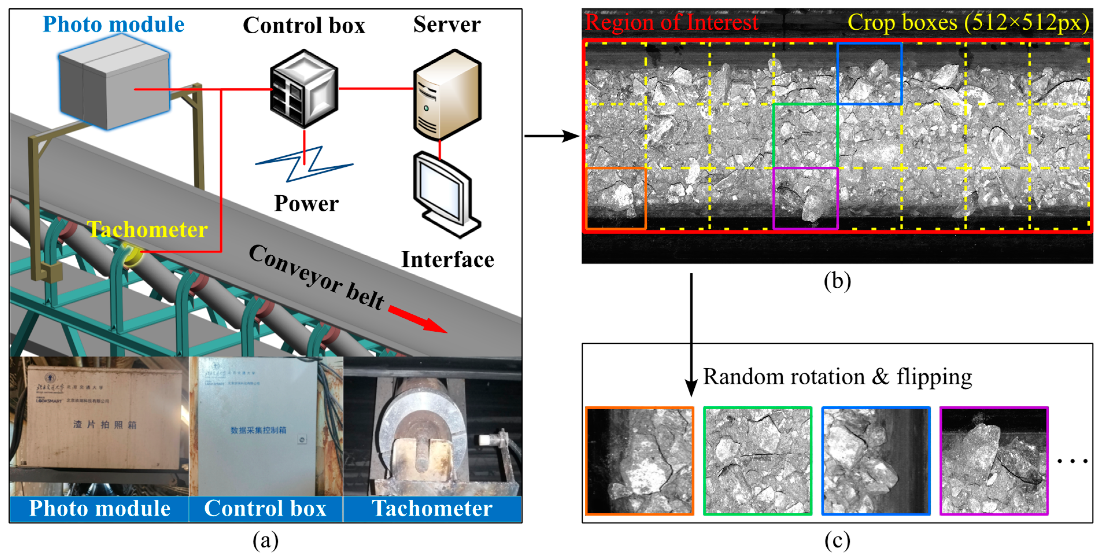
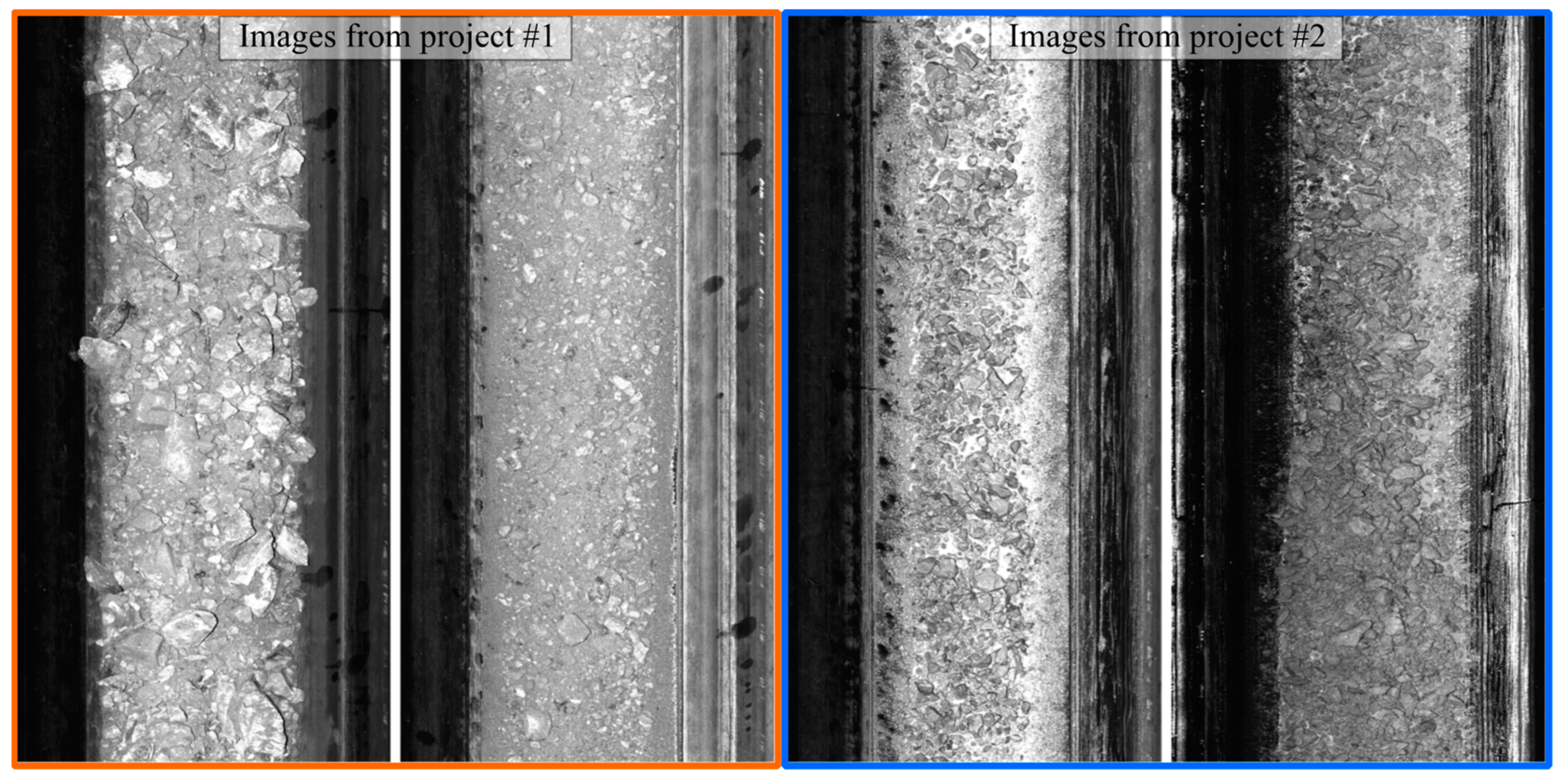
The muck images that had been used for training the MuckSeg-SS-FCMAE had been captured using a photography system depicted in Figure 11a. This system was primarily composed of a photo module, a control box, a tachometer, and a server. The linear array camera within the photo module could capture high-resolution, clear images of the high-speed moving muck chip on the conveyor belt, aided by a laser light source. The control box would adjust the camera’s line frequency in real-time, based on the conveyor belt’s speed as measured using the tachometer, to prevent size distortion. The muck images’ resolution along the camera’s scanning line direction was 2048 pixels, capturing and saving an 8-bit grayscale image every 4096 pixels. To enhance the generalization capability of the model, the muck images in the dataset were collected from two different projects, with specific details provided in Table 3, and examples of the collected muck images can be seen in Figure 12. In total, over 40,000 full-size muck images were used to establish the training dataset.
As shown in Figure 11b,c, once training commenced, the ROI in the middle of the full-size muck image, measuring 1536 × 4096 pixels, was divided into 24 crop boxes of 512 × 512. A single crop box was selected at random for extracting the training sample from the ROI. Given the already substantial volume of data, no additional data augmentation techniques were employed beyond random rotation and flipping.

3. Experiments and Results

3.1. Experiment Environment

3.1.1. Hardware Specifications

  • CPU: AMD Ryzen 9 5950X 16-core processor.
  • GPU: Nvidia GeForce RTX 4090.
  • RAM: 64GB DDR4 at 3200 MHz.

3.1.2. Software Environment

  • Operating system: Ubuntu 22.04.
  • Programming language: Python 3.9.13.
  • Deep Learning Framework: PyTorch 2.0.1 with Lightning 2.0.1.
  • Sparse convolution operator library: MinkowskiEngine 0.5.4.

3.2. Evaluation Criteria

In this section, we will thoroughly evaluate the MuckSeg-SS-FCMAE model’s effectiveness in three key areas:
  • Image reconstruction capability. The autoencoder’s ability to reconstruct images is a vital metric for determining if the learned representations hold enough information to replicate the original input. This reflects not only the model’s grasp of the input data’s structure but also its ability to identify essential features.
  • Feature extraction capability of the MAE encoder. The MAE is designed to empower the encoder to identify fundamental image features autonomously. This positions the model at a more advantageous starting point in the parameter space for downstream tasks, increasing the likelihood of optimal parameter convergence and reducing the risk of entrapment in local minima. Furthermore, exposing the encoder to a broader dataset enhances the model’s generalization and robustness. Thus, the MAE encoder’s proficiency in discerning target feature semantics is crucial for gauging MAE’s effectiveness.
  • Performance improvement when transferring to downstream tasks. The MAE’s impact on muck segmentation tasks is most directly observed by comparing the improvements in the IoU of boundary and region labels predicted by the pre-trained network against those trained from scratch. The IoU is calculated as follows:
    IoU = TP FP + TP + FN
    where TP denotes the total number of true positive samples, FP the false positives, and FN the false negatives.

3.3. Training Procedure

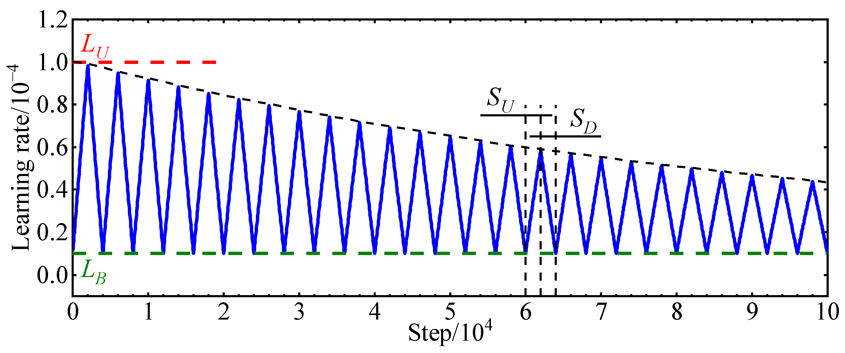
Before training commenced, all the weights in the model were initialized using a standard normal distribution with a standard deviation of 0.02, and the sampled values were constrained within the [−2, 2] interval. All biases were set to zero. To achieve better optimization effects, the model employed the AdamW optimizer [44]. Additionally, to maintain a balance between exploration and optimization in the parameter space throughout the training, a cyclic learning rate schedule [45] is employed. As illustrated in Figure 13, this scheduler modulates the learning rate between a lower limit LB and a gradually dampened upper limit LU. Starting from LB, the rate linearly increases to current LU’ = ζnLU over SU mini-batches, where ζ denotes the damping coefficient and n is the current step count, then decreases back to LB across SD batches, completing one cycle. This process is repeated, facilitating the network’s ability to escape local minima and explore various parameter spaces, ultimately improving the chances of reaching a superior solution and enhancing performance.
All training hyperparameters can be found in Table 4.
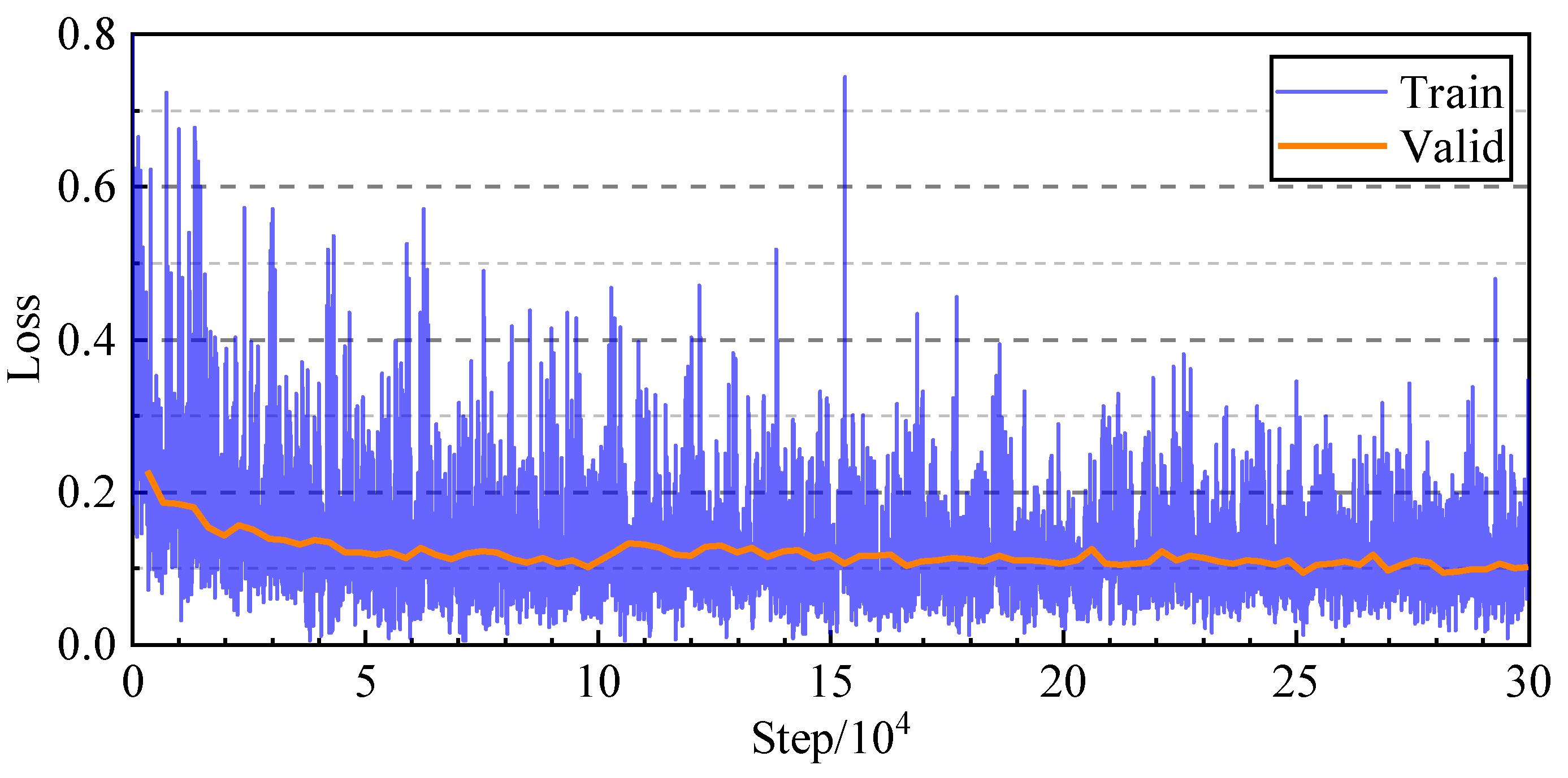
The loss curves during the training process are shown in Figure 14. To monitor whether the model was overfitting, the average loss was evaluated using a validation set comprising 100 muck images independent of the training dataset every 3000 steps during training, which is represented by a thick orange line in the figure. It can be observed from the graph that the learning speed of SS-FCMAE is relatively low, and there are large fluctuations in the loss. The downward trend of the loss curve becomes less apparent after approximately 100,000 steps, but experiments have shown that there is still considerable room for improvement in model performance at this point, which can also be confirmed by the slow downward trend of the training curve in the later stages. It is not difficult to notice that, even after more than 200,000 steps, the loss curves for the training and validation sets still highly overlap, indicating that SS-FCMAE is unlikely to overfit when applied to muck images. Conversely, underfitting is a more pressing issue that needs attention, and appropriately extending the training time is beneficial for model performance.

3.4. Image Reconstruction Capability

This section analyzes the image reconstruction capabilities of both the original FCMAE and the MuckSeg-SS-FCMAE, in addition to training an SS-FCMAE without the use of HOG descriptors and Laplacian feature supervision for further comparison.
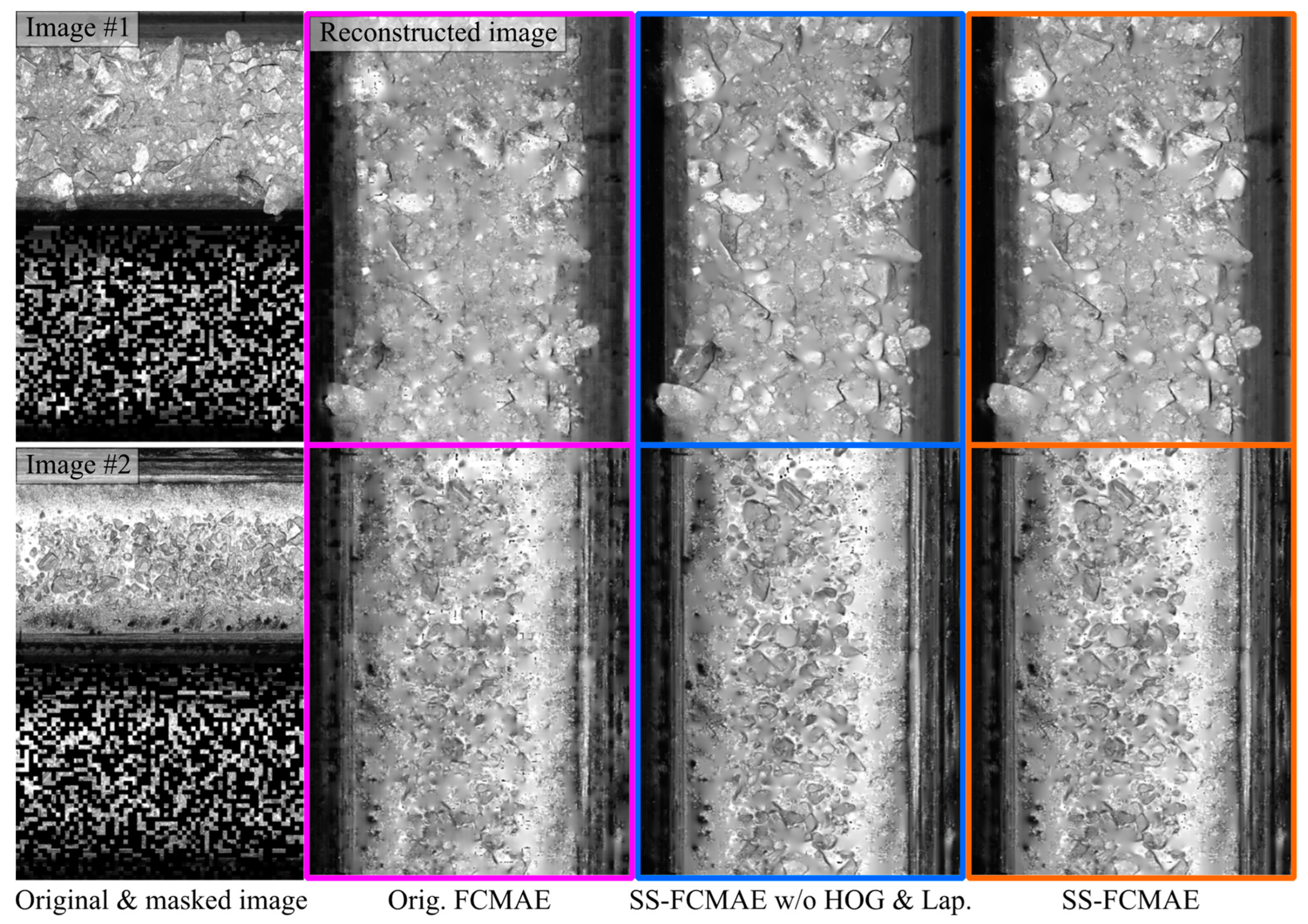
Figure 15 presents a comparative analysis of image reconstruction capabilities across the three models. It is evident that all three FCMAE schemes effectively restore the global contrast and the approximate contours of the main muck chip bodies, demonstrating FCMAE’s strong global comprehension of muck images and its ability to capture the images’ macroscopic characteristics. When examining the details within the masked areas, the SS-FCMAE notably excels in reconstructing muck boundaries that are partially obscured or nearly invisible, a critical aspect for subsequent muck segmentation tasks. The transitions between reconstructed masked areas and the original unmasked areas appear seamless with the SS-FCMAE, showcasing its superior capability in learning local texture features. In contrast, the original FCMAE tends to smooth over local pixel values in masked areas, leading to a vague, uniform texture in the reconstructions, which aligns with the trivial solutions mentioned in Section 3.4 and may account for the original FCMAE’s limited training performance.
The SS-FCMAE’s image reconstruction did not exhibit notable differences in the absence of HOG descriptors and Laplacian features, suggesting that the model’s convolutional structure alone might have sufficed for the general reconstruction of muck images. Nevertheless, it is important to recognize that both the original FCMAE and SS-FCMAE have their limitations in reconstructing large continuous masked areas and pixel-level details. Although increasing the network’s depth and width could potentially address this, the balance between model performance and computational cost must be considered. Despite these challenges, the image reconstruction capabilities of MuckSeg-SS-FCMAE are deemed satisfactory.

3.5. Feature Extraction Capability

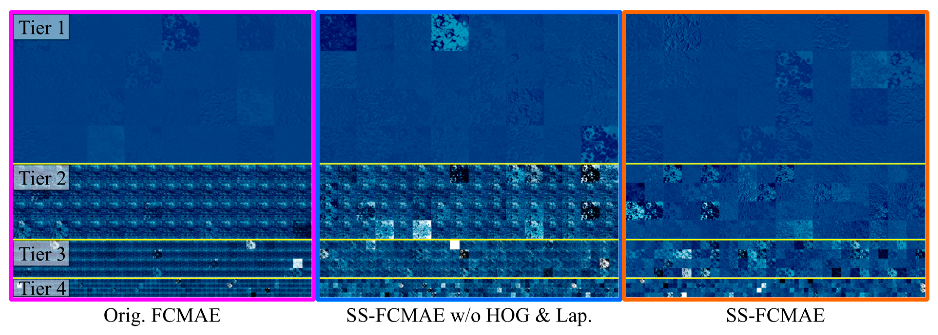
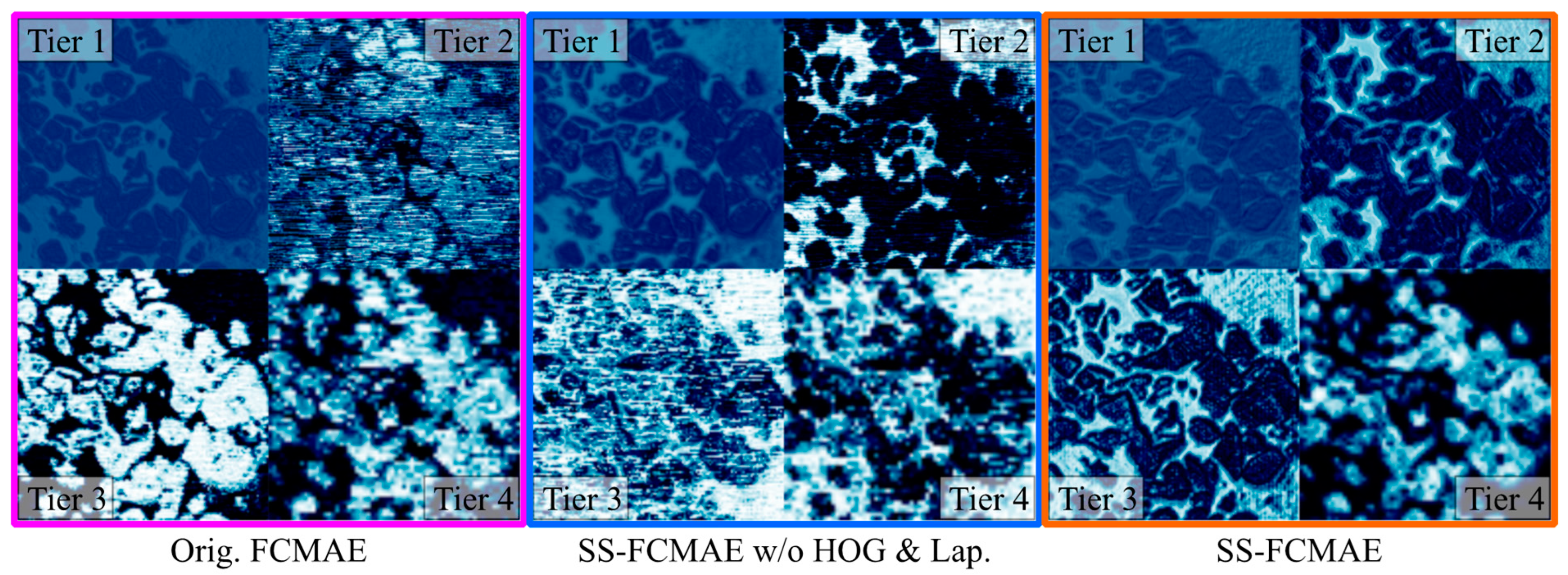
To assess the feature extraction capability of the FCMAE encoders, this section directly inputs an unmasked image into the FCMAEs and extracts the feature maps from the last ConvNeXt block of each of the four encoder tiers under each scheme. The visualization results are presented in Figure 16 and Figure 17. It is evident from these figures that the first encoder tier of all schemes has somewhat learned to differentiate between muck chip regions and the background, with the SS-FCMAE producing clearer feature maps than other schemes, thus capturing the image’s primary information more effectively. However, from the second tier onwards, the feature maps under the three schemes begin to diverge significantly. Figure 16 shows that the neurons in the second to fourth encoder tiers of the SS-FCMAE are effectively activated, demonstrating clear channel differentiation in the feature maps. This indicates that the encoder’s learning capabilities are maximized, facilitating the extraction of a richer and more varied feature set for describing the muck images.
Conversely, the SS-FCMAE encoder, which does not employ HOG descriptors and Laplacian features, exhibits noticeable noise in the outputs of the intermediate tiers, potentially disrupting subsequent muck segmentation tasks. Moreover, approximately 70% of the feature dimensions were highly similar, suggesting that many neurons have learned identical weights. Such redundancy not only demonstrates the model’s failure to capture sufficiently valuable information but also undermines its learning capacity. Noticeable saturation of neurons is observed in the third and fourth encoder tiers, adversely affecting network performance. The original MAE displays even more pronounced issues, with outputs on nearly 90% of the channels in the feature maps being almost entirely identical; even on the few valuable channels, the feature maps show noticeable noise and unidirectional textures.
In conclusion, the SS-FCMAE shows a greater aptitude for learning valuable information from muck images via self-supervised training compared to the original FCMAE. The addition of HOG descriptors and Laplacian features as training targets notably enhances the learning capability of the deeper encoder tiers and reduces feature channel redundancy.

3.6. Improvement on Segmentation Results

In this section, the pre-trained weights from the three previously mentioned schemes were transferred to the MuckSeg main network and fine-tuned using a dataset created from 70 finely annotated full-size muck images, using a base learning rate of 2 × 10⁻⁴ for 60 epochs. Additionally, another MuckSeg model was trained from scratch as a baseline to assess the performance improvements of various types of masked autoencoders on the downstream muck segmentation task. Moreover, the current state-of-the-art (SOTA) muck segmentation model—MSD-UNet [22]—was also replicated and trained on our dataset according to the original research methods for comparison with the approach presented in this paper. The average IoU was then calculated for these models using the test dataset.
Table 5 presents the average IoU of each model on the test dataset. The table indicates that, when using only the pixel values of input images for self-supervision, the SS-FCMAE’s predicted IoU for muck boundaries and regions increased by approximately 4.6% and 1.8%, respectively, compared to the baseline. Incorporating HOG descriptors and Laplacian features as additional supervision targets further enhanced the model’s performance, yielding improvements of 5.9% and 2.4% over the baseline. In contrast, the original FCMAE showed more modest gains of 1.9% and 1.2%. Furthermore, without the use of MAE pre-training, our model’s performance on the test set was only marginally better than that of MSD-UNet. However, after incorporating SS-FCMAE, MuckSeg achieved an improvement of 8.3% and 4.7% over MSD-UNet, which is crucial for enhancing the accuracy of muck gradation calculations.
Figure 18 illustrates the error maps of prediction results from the various models discussed in this section. It was observed that our model, when trained from scratch, performs similarly to MSD-UNet on relatively simple samples, such as image #2. However, for image #1, MSD-UNet experiences significant deficiencies in predicting muck regions and struggles to identify the complete boundaries of large muck chips, whereas our model shows relatively better performance. The addition of MAE pre-training further enhances the integrity of the model’s predictions for muck chip regions and boundaries to various extents. Specifically, the SS-FCMAE, which included HOG descriptors and Laplacian features, achieved very satisfactory results. However, some noise was noted in the SS-FCMAE’s output, suggesting that the model might have overfitted to the texture features of the muck to some extent. Despite this overfitting being undesirable, it also indirectly shows that SS-FCMAE pre-training has bolstered the model’s ability to discern smaller-scale features, without affecting the final segmentation results.

3.7. Hyperparameter Optimization

In the context of real-time surrounding rock perception technology, our model must address computational constraints and ensure processing efficiency within the TBM construction environment. This section will, therefore, examine how hyperparameter variations influence model performance and computational costs. Beyond hyperparameters pertaining to the loss function and training regimen, our model’s adjustable hyperparameters are broadly categorized as follows:
  • Non-independent hyperparameters include the following:
    • The dimension of the feature map produced by the stem block, denoted as D.
    • The count of ConvNeXt blocks in each encoder tier, denoted as Nei for i = 1, 2, 3, and 4.
Given that the stem block and encoder in MuckSeg-SS-FCMAE must align with the MuckSeg main network, alterations to these hyperparameters affect not only MAE performance but also the downstream end-to-end fine-tuning outcomes. Consequently, we use the IoU of the final end-to-end model on the test dataset as the metric for evaluating these hyperparameters. It is important to note that due to the time-intensive nature of MAE training, we base our evaluation and adjustment of these hyperparameters on models trained from scratch.
2.
Independent hyperparameters include the following:
  • The feature dimension of the mask token, denoted as Dm.
  • The count of ConvNeXt blocks in each MAE decoder tier, denoted as Ndi for i = 1 and 2.
  • The count of ConvNeXt blocks in the MAE neck, denoted as Nn.
These hyperparameters solely impact MAE performance. Therefore, we assess them using the IoU improvement on the test dataset when MAE pre-training is applied, as opposed to training from scratch.
On the other hand, computational costs are assessed from two perspectives:
  • The number of model parameters, measured in millions of parameters (MParams).
  • The computational cost of processing a single sample, measured in billions of floating-point operations (GFLOPs).
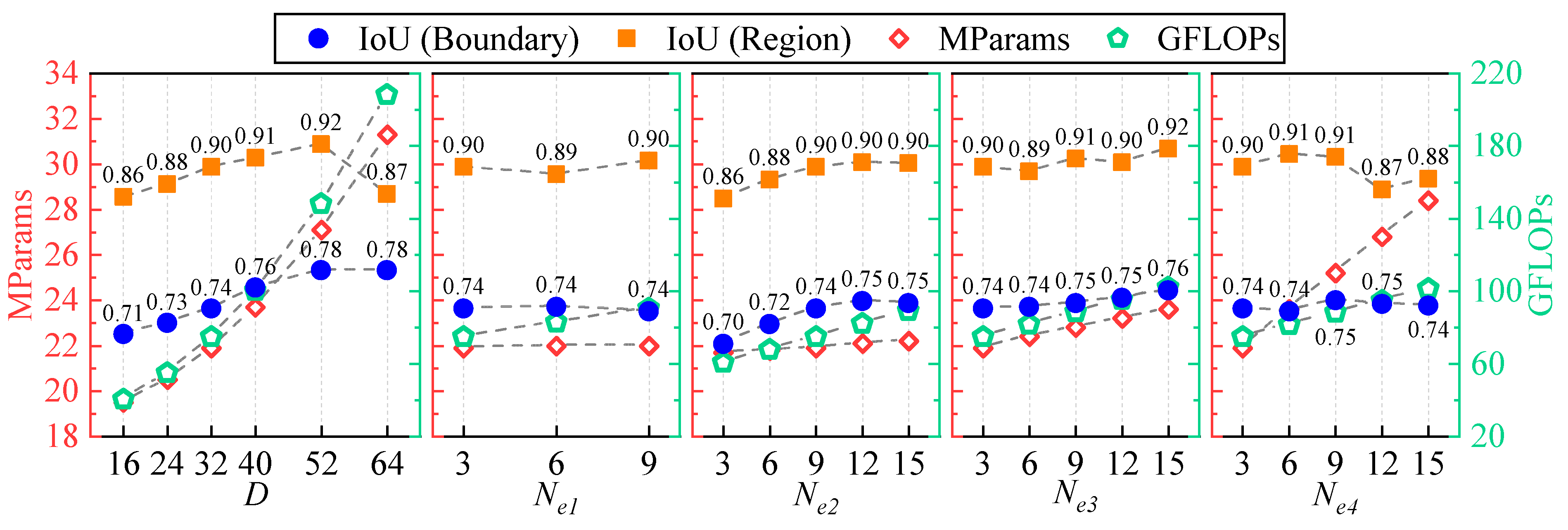
The analyzes in this section utilize the default configuration (D = 32, Nei = {3, 9, 3, 3}, Dm = 512, and Ndi = {2, 2}, Nn = 8) as a baseline. Figure 19 presents the performance and computational costs of MuckSeg-SS-FCMAE with various non-independent hyperparameters. It is evident that D significantly influences the computational cost of the model. Correspondingly, increasing D also notably improves the model’s performance, especially in the prediction accuracy of muck chip boundaries. When D exceeds 32, the computational cost rises steeply, while the enhancement in model performance becomes relatively modest. Conversely, variations in Nei do not generally affect model performance significantly, except for a marked improvement when Ne2 increases from 3 to 9. This suggests that features at this scale are crucial in muck segmentation tasks. The performance gains from increasing Nei at other tiers are not cost-effective. Thus, the final configuration selected for the proposed model is D = 32 and Nei = {3, 9, 3, 3}.
Figure 20 illustrates the changes in model performance and computational cost with different independent hyperparameters. It is apparent that incorporating only one ConvNeXt block in each tier of the SS-FCMAE decoder leads to a decline in its performance, and adding more than two layers does not significantly enhance performance, even causing degradation when increased to four layers. This suggests that an overly powerful decoder in the SS-FCMAE can actually impair the encoder’s learning ability. In contrast, the design of the neck in the SS-FCMAE is quite critical. Specifically, the number of ConvNeXt blocks in the neck, Nn, should be more than eight to ensure adequate feature interaction between masked and unmasked regions. The dimension of the mask token, Dm, should align with the feature map dimension, which is 512 in the default configuration, produced by the encoder. Reducing the feature dimension of the encoder’s output can lead to a decline in MAE performance and may even negatively impact downstream tasks, while the additional computational cost of expanding the feature dimension is almost negligible. In conclusion, the final configuration selected for the proposed model is Dm = 512, Nn = 8, and Ndi = {2, 2}.

4. Discussion

This study has highlighted the significant role of MAE self-supervised pre-training in muck segmentation tasks, as well as the notable performance gains achieved by the SS-FCMAE designed for this task. However, due to the limited sources of muck images, it is currently uncertain whether the model presented in this paper has general applicability to different types of rocks, different TBMs, and different photography equipment. It is hoped that in the future, more researchers will devote themselves to research in this field and achieve widespread data sharing to establish a more substantial and diverse muck image dataset. Furthermore, while self-supervised pre-training has somewhat mitigated the challenge of limited labeled data, the SS-FCMAE still relies on comprehensive end-to-end fine-tuning to function effectively. Consequently, the burdensome costs of annotation and the scarcity of labeled data in muck segmentation tasks remain pressing issues.
Recent developments underscore the importance of self-supervised learning techniques across various domains for the advancement and deployment of deep learning models. In the field of NLP, self-supervised learning has become foundational, enabling the construction of large models with robust generalization abilities. However, in the field of CV, despite the introduction of MAE and joint embedding methods enhancing the practicality of self-supervised training, these frameworks have yet to achieve the same level of autonomy as in NLP. Considering the distinct differences between image and natural language data, and the fact that current CV self-supervised training approaches have been largely inspired by NLP, there is a compelling need to develop self-supervised methods that are intrinsically suited to the unique demands of CV tasks.
Moreover, our research suggests that combining traditional image processing techniques with modern deep learning can lead to remarkably effective outcomes, especially in self-supervised learning contexts. Techniques such as HOG descriptors, previously central to feature engineering, can still offer valuable insights. Future research should continue to investigate how these once-prevalent methods can be reinvigorated within the deep learning paradigm.
Furthermore, the advent of multi-modal and large-scale CV models, such as Segment Anything [46], promises significant advancements in domain-specific tasks like muck segmentation through the use of these foundational models. The prospective fusion of CV tasks with such models could transcend conventional approaches, including knowledge distillation, representing a research avenue of substantial potential.

5. Conclusions

In this study, we introduce the MuckSeg-SS-FCMAE, a semi-symmetric, fully convolutional masked autoencoder tailored for TBM muck segmentation tasks. The model employs a multi-layer parallel sparse decoder to up-sample and decode masked feature maps, which enables it to capture the relative positional relationships between pixels, enhancing its extraction of low-level geometric features such as muck chip geometry and boundaries. By integrating HOG descriptors and Laplacian features—rapidly obtainable prior features through classical algorithms—as additional self-supervision targets, our approach effectively circumvents the trivial solution problem inherent in relying solely on pixel value MSE loss and diminishes network neuron redundancy. Our experiments demonstrate that the MuckSeg-SS-FCMAE outperforms the original MAE in learning from muck images and that the inclusion of HOG descriptors and Laplacian features bolsters self-supervised training, maximizing the encoder’s learning potential. Moreover, pre-training with MuckSeg-SS-FCMAE significantly enhances the accuracy, generalization, and robustness of the subsequently trained muck segmentation network compared to training from scratch.

Author Contributions

Conceptualization and project administration, Z.T. and X.W.; resources and funding acquisition, Z.T.; data curation and validation, Z.Z.; investigation, methodology, software, formal analysis, visualization, and writing—original draft, K.L.; writing—review and editing, X.W. All authors have read and agreed to the published version of the manuscript.

Funding

This research was funded by the Science and Technology Major Project of Xinjiang Uygur Autonomous Region [grant number: 2020A03003-5] and the China Postdoctoral Science Foundation [certificate number: 2023M730204].

Data Availability Statement

The source code for the project can be accessed at the following GitHub repository: https://github.com/leike0813/MuckSeg_FCMAE (accessed on 18 January 2024). For access to a detailed dataset, please contact [email protected].

Acknowledgments

The authors are grateful to China Railway 16th Bureau Group Co., Ltd., Beijing, China and CCCC Second Highway Engineering Co., Ltd., Xi’an, China for their cooperation in image acquisition.

Conflicts of Interest

The image acquisition device used in this study was developed by Beijing JiuRui Technology Co., Ltd. The authors declare that they have no financial interest in the company or in the commercialization of this equipment.

References

  1. Li, J.B.; Jing, L.J.; Zheng, X.F.; Li, P.Y.; Yang, C. Application and Outlook of Information and Intelligence Technology for Safe and Efficient TBM Construction. Tunn. Undergr. Space Technol. 2019, 93, 103097. [Google Scholar] [CrossRef]
  2. Li, J.B.; Chen, Z.Y.; Li, X.; Jing, L.J.; Zhang, Y.P.; Xiao, H.H.; Wang, S.J.; Yang, W.K.; Wu, L.J.; Li, P.Y.; et al. Feedback on a Shared Big Dataset for Intelligent TBM Part I: Feature Extraction and Machine Learning Methods. Undergr. Space 2023, 11, 1–25. [Google Scholar] [CrossRef]
  3. Liu, B.; Wang, J.W.; Wang, R.R.; Wang, Y.X.; Zhao, G.Z. Intelligent Decision-Making Method of TBM Operating Parameters Based on Multiple Constraints and Objective Optimization. J. Rock Mech. Geotech. Eng. 2023, 15, 2842–2856. [Google Scholar] [CrossRef]
  4. Guo, D.; Li, J.H.; Jiang, S.H.; Li, X.; Chen, Z.Y. Intelligent Assistant Driving Method for Tunnel Boring Machine Based on Big Data. Acta Geotech. 2022, 17, 1019–1030. [Google Scholar] [CrossRef]
  5. Zhang, Y.K.; Gong, G.F.; Yang, H.Y.; Chen, Y.X.; Chen, G.L. Towards Autonomous and Optimal Excavation of Shield Machine: A Deep Reinforcement Learning-Based Approach. J. Zhejiang Univ. Sci. A 2022, 23, 458–478. [Google Scholar] [CrossRef]
  6. Yokota, Y.; Yamamoto, T.; Shirasagi, S.; Koizumi, Y.; Descour, J.; Kohlhaas, M. Evaluation of Geological Conditions Ahead of TBM Tunnel Using Wireless Seismic Reflector Tracing System. Tunn. Undergr. Space Technol. 2016, 57, 85–90. [Google Scholar] [CrossRef]
  7. Li, C.S.; Gu, T.; Ding, J.F.; Yu, W.G.; He, F.L. Horizontal Sound Probing (HSP) Geology Prediction Method Appropriated to Tbm Construction. J. Eng. Geol. 2008, 16, 111–115. [Google Scholar]
  8. Li, S.C.; Nie, L.C.; Liu, B. The Practice of Forward Prospecting of Adverse Geology Applied to Hard Rock TBM Tunnel Construction: The Case of the Songhua River Water Conveyance Project in the Middle of Jilin Province. Engineering 2018, 4, 131–137. [Google Scholar] [CrossRef]
  9. Kaus, A.; Boening, W. BEAM—Geoelectrical Ahead Monitoring for TBM-Drives. Geomech. Tunn. 2008, 1, 442–449. [Google Scholar] [CrossRef]
  10. Mohammadi, M.; Khademi Hamidi, J.; Rostami, J.; Goshtasbi, K. A Closer Look into Chip Shape/Size and Efficiency of Rock Cutting with a Simple Chisel Pick: A Laboratory Scale Investigation. Rock Mech. Rock Eng. 2020, 53, 1375–1392. [Google Scholar] [CrossRef]
  11. Tuncdemir, H.; Bilgin, N.; Copur, H.; Balci, C. Control of Rock Cutting Efficiency by Muck Size. Int. J. Rock Mech. Min. Sci. 2008, 45, 278–288. [Google Scholar] [CrossRef]
  12. Heydari, S.; Khademi Hamidi, J.; Monjezi, M.; Eftekhari, A. An Investigation of the Relationship between Muck Geometry, TBM Performance, and Operational Parameters: A Case Study in Golab II Water Transfer Tunnel. Tunn. Undergr. Space Technol. 2019, 88, 73–86. [Google Scholar] [CrossRef]
  13. Barron, L.; Smith, M.L.; Prisbrey, K. Neural Network Pattern Recognition of Blast Fragment Size Distributions. Part. Sci. Technol. 1994, 12, 235–242. [Google Scholar] [CrossRef]
  14. Jemwa, G.T.; Aldrich, C. Estimating Size Fraction Categories of Coal Particles on Conveyor Belts Using Image Texture Modeling Methods. Expert Syst. Appl. 2012, 39, 7947–7960. [Google Scholar] [CrossRef]
  15. Rispoli, A.; Ferrero, A.M.; Cardu, M.; Farinetti, A. Determining the Particle Size of Debris from a Tunnel Boring Machine Through Photographic Analysis and Comparison Between Excavation Performance and Rock Mass Properties. Rock Mech. Rock Eng. 2017, 50, 2805–2816. [Google Scholar] [CrossRef]
  16. Abu Bakar, M.Z.; Gertsch, L.S.; Rostami, J. Evaluation of Fragments from Disc Cutting of Dry and Saturated Sandstone. Rock Mech. Rock Eng. 2014, 47, 1891–1903. [Google Scholar] [CrossRef]
  17. Al-Thyabat, S.; Miles, N.J.; Koh, T.S. Estimation of the Size Distribution of Particles Moving on a Conveyor Belt. Miner. Eng. 2007, 20, 72–83. [Google Scholar] [CrossRef]
  18. Chen, H.A.; Jin, Y.; Li, G.Q.; Chu, B. Automated Cement Fragment Image Segmentation and Distribution Estimation via a Holistically-Nested Convolutional Network and Morphological Analysis. Powder Technol. 2018, 339, 306–313. [Google Scholar] [CrossRef]
  19. Liu, H.Q.; Yao, M.B.; Xiao, X.M.; Xiong, Y.G. RockFormer: A U-Shaped Transformer Network for Martian Rock Segmentation. IEEE Trans. Geosci. Remote Sens. 2023, 61, 4600116. [Google Scholar] [CrossRef]
  20. Fan, L.L.; Yuan, J.B.; Niu, X.W.; Zha, K.K.; Ma, W.Q. RockSeg: A Novel Semantic Segmentation Network Based on a Hybrid Framework Combining a Convolutional Neural Network and Transformer for Deep Space Rock Images. Remote Sens. 2023, 15, 3935. [Google Scholar] [CrossRef]
  21. Liang, Z.Y.; Nie, Z.H.; An, A.J.; Gong, J.; Wang, X. A Particle Shape Extraction and Evaluation Method Using a Deep Convolutional Neural Network and Digital Image Processing. Powder Technol. 2019, 353, 156–170. [Google Scholar] [CrossRef]
  22. Zhou, X.X.; Gong, Q.M.; Liu, Y.Q.; Yin, L.J. Automatic Segmentation of TBM Muck Images via a Deep-Learning Approach to Estimate the Size and Shape of Rock Chips. Autom. Constr. 2021, 126, 103685. [Google Scholar] [CrossRef]
  23. Vincent, P.; Larochelle, H.; Bengio, Y.; Manzagol, P.-A. Extracting and Composing Robust Features with Denoising Autoencoders. In Proceedings of the 25th International Conference on Machine Learning, Helsinki, Finland, 5–9 July 2008; pp. 1096–1103. [Google Scholar]
  24. Pathak, D.; Krahenbuhl, P.; Donahue, J.; Darrell, T.; Efros, A.A. Context Encoders: Feature Learning by Inpainting. In Proceedings of the IEEE Conference on Computer Vision and Pattern Recognition, Las Vegas, NV, USA, 26 June–1 July 2016; pp. 2536–2544. [Google Scholar]
  25. Baevski, A.; Hsu, W.N.; Xu, Q.; Babu, A.; Gu, J.; Auli, M. Data2vec: A General Framework for Self-Supervised Learning in Speech, Vision and Language. In Proceedings of the 39th International Conference on Machine Learning; PMLR, Baltimore, MD, USA, 28 June 2022; pp. 1298–1312. [Google Scholar]
  26. Assran, M.; Caron, M.; Misra, I.; Bojanowski, P.; Bordes, F.; Vincent, P.; Joulin, A.; Rabbat, M.; Ballas, N. Masked Siamese Networks for Label-Efficient Learning. In Proceedings of the Computer Vision—ECCV, Tel Aviv, Israel, 23–27 October 2022; Avidan, S., Brostow, G., Cissé, M., Farinella, G.M., Hassner, T., Eds.; Springer Nature: Cham, Switzerland, 2022; pp. 456–473. [Google Scholar]
  27. He, K.M.; Fan, H.Q.; Wu, Y.X.; Xie, S.N.; Girshick, R. Momentum Contrast for Unsupervised Visual Representation Learning. In Proceedings of the IEEE/CVF Conference on Computer Vision and Pattern Recognition, Seattle, WA, USA, 13–19 June 2020; pp. 9729–9738. [Google Scholar]
  28. Chen, T.; Kornblith, S.; Norouzi, M.; Hinton, G. A Simple Framework for Contrastive Learning of Visual Representations. In Proceedings of the 37th International Conference on Machine Learning; PMLR, Virtual Event, 13–18 July 2020; pp. 1597–1607. [Google Scholar]
  29. Dong, X.Y.; Bao, J.M.; Zhang, T.; Chen, D.D.; Zhang, W.M.; Yuan, L.; Chen, D.; Wen, F.; Yu, N.H.; Guo, B.N. PeCo: Perceptual Codebook for BERT Pre-Training of Vision Transformers. In Proceedings of the AAAI Conference on Artificial Intelligence, Washington, DC, USA, 7–14 February 2023; Volume 37, pp. 552–560. [Google Scholar] [CrossRef]
  30. Kenton, J.D.M.-W.C.; Toutanova, L.K. Bert: Pre-Training of Deep Bidirectional Transformers for Language Understanding. In Proceedings of the Naacl-HLT, Minneapolis, MN, USA, 2–7 June 2019; Volume 1, p. 2. [Google Scholar]
  31. Bao, H.B.; Dong, L.; Piao, S.H.; Wei, F.R. BEiT: BERT Pre-Training of Image Transformers. arXiv 2023, arXiv:2106.08254. [Google Scholar] [CrossRef]
  32. Dong, X.Y.; Bao, J.M.; Zhang, T.; Chen, D.D.; Zhang, W.M.; Yuan, L.; Chen, D.; Wen, F.; Yu, N.H. Bootstrapped Masked Autoencoders for Vision BERT Pretraining. In Proceedings of the Computer Vision—ECCV, Tel Aviv, Israel, 23–27 October 2022; Avidan, S., Brostow, G., Cissé, M., Farinella, G.M., Hassner, T., Eds.; Springer Nature: Cham, Switzerland, 2022; pp. 247–264. [Google Scholar]
  33. He, K.M.; Chen, X.L.; Xie, S.N.; Li, Y.H.; Dollár, P.; Girshick, R. Masked Autoencoders Are Scalable Vision Learners. In Proceedings of the IEEE/CVF Conference on Computer Vision and Pattern Recognition, New Orleans, LA, USA, 18–24 June 2022; pp. 16000–16009. [Google Scholar]
  34. Xie, Z.D.; Zhang, Z.; Cao, Y.; Lin, Y.T.; Bao, J.M.; Yao, Z.L.; Dai, Q.; Hu, H. SimMIM: A Simple Framework for Masked Image Modeling. In Proceedings of the 37th International Conference on Machine Learning, Virtual Event, 13–18 July 2022; pp. 9653–9663. [Google Scholar]
  35. Cai, Z.X.; Ghosh, S.; Stefanov, K.; Dhall, A.; Cai, J.F.; Rezatofighi, H.; Haffari, R.; Hayat, M. MARLIN: Masked Autoencoder for Facial Video Representation LearnINg. In Proceedings of the IEEE/CVF Conference on Computer Vision and Pattern Recognition, Vancouver, BC, Canada, 17–24 June 2023; pp. 1493–1504. [Google Scholar]
  36. Pang, Y.T.; Wang, W.X.; Tay, F.E.H.; Liu, W.; Tian, Y.H.; Yuan, L. Masked Autoencoders for Point Cloud Self-Supervised Learning. In Proceedings of the Computer Vision—ECCV, Tel Aviv, Israel, 23–27 October 2022; Avidan, S., Brostow, G., Cissé, M., Farinella, G.M., Hassner, T., Eds.; Springer Nature: Cham, Switzerland, 2022; pp. 604–621. [Google Scholar]
  37. Reed, C.J.; Gupta, R.; Li, S.; Brockman, S.; Funk, C.; Clipp, B.; Keutzer, K.; Candido, S.; Uyttendaele, M.; Darrell, T. Scale-MAE: A Scale-Aware Masked Autoencoder for Multiscale Geospatial Representation Learning. In Proceedings of the IEEE/CVF International Conference on Computer Vision, Vancouver, BC, Canada, 17–24 June 2023; pp. 4088–4099. [Google Scholar]
  38. Dalal, N.; Triggs, B. Histograms of Oriented Gradients for Human Detection. In Proceedings of the 2005 IEEE Computer Society Conference on Computer Vision and Pattern Recognition (CVPR’05), San Diego, CA, USA, 25–26 June 2005; Volume 1, pp. 886–893. [Google Scholar]
  39. Ramesh, A.; Pavlov, M.; Goh, G.; Gray, S.; Voss, C.; Radford, A.; Chen, M.; Sutskever, I. Zero-Shot Text-to-Image Generation. In Proceedings of the 38th International Conference on Machine Learning; PMLR, Virtual Event, 18–24 July 2021; pp. 8821–8831. [Google Scholar]
  40. Vaswani, A.; Shazeer, N.; Parmar, N.; Uszkoreit, J.; Jones, L.; Gomez, A.N.; Kaiser, Ł.; Polosukhin, I. Attention Is All You Need. In Proceedings of the Advances in Neural Information Processing Systems, Long Beach, CA, USA, 4–9 December 2017; Guyon, I., Luxburg, U.V., Bengio, S., Wallach, H., Fergus, R., Vishwanathan, S., Garnett, R., Eds.; Curran Associates, Inc.: New York, NY, USA, 2017; Volume 30. [Google Scholar]
  41. Woo, S.; Debnath, S.; Hu, R.H.; Chen, X.L.; Liu, Z.; Kweon, I.S.; Xie, S.N. ConvNeXt V2: Co-Designing and Scaling ConvNets with Masked Autoencoders 2023. In Proceedings of the IEEE/CVF Conference on Computer Vision and Pattern Recognition, New Orleans, LA, USA, 18–24 June 2022; pp. 11976–11986. [Google Scholar]
  42. Graham, B.; van der Maaten, L. Submanifold Sparse Convolutional Networks. arXiv 2023, arXiv:1706.01307. [Google Scholar] [CrossRef]
  43. Deng, M.J. Challenges and Thoughts on Risk Management and Control for the Group Construction of a Super-Long Tunnel by TBM. Engineering 2018, 4, 112–122. [Google Scholar] [CrossRef]
  44. Loshchilov, I.; Hutter, F. Decoupled Weight Decay Regularization. arXiv 2023, arXiv:1711.05101. [Google Scholar] [CrossRef]
  45. Smith, L.N. Cyclical Learning Rates for Training Neural Networks. In Proceedings of the 2017 IEEE Winter Conference on Applications of Computer Vision (WACV), Santa Rosa, CA, USA, 17–24 March 2017; pp. 464–472. [Google Scholar]
  46. Kirillov, A.; Mintun, E.; Ravi, N.; Mao, H.; Rolland, C.; Gustafson, L.; Xiao, T.; Whitehead, S.; Berg, A.C.; Lo, W.-Y.; et al. Segment Anything. arXiv 2023, arXiv:2304.02643. [Google Scholar] [CrossRef]
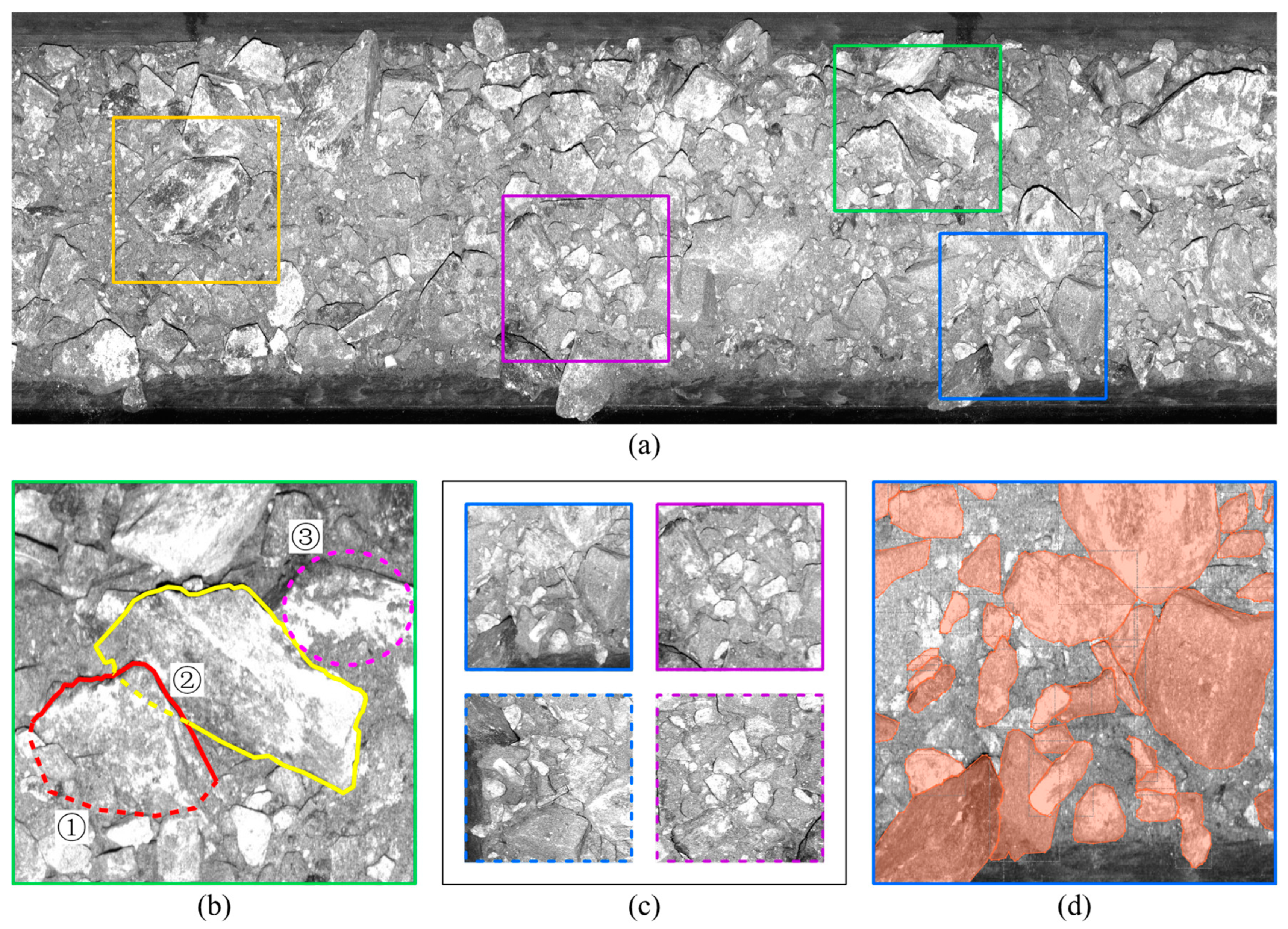
Figure 1. Characteristics of TBM muck image. (a) A sample muck image collected during TBM advancing. (b) The muck chips may present unfavorable characteristics such as the following: ① Invisible boundary; ② Overlapping; ③ Confusing texture. (c) The local image indicated by the blue and violet boxes, with the dashed boxes showing the results after rotation. (d) Muck chip annotations in blue box.
Symmetry 16 00222 g001
Figure 2. Overview of masked autoencoders using the figure borrowed from the original work [33].
Symmetry 16 00222 g002
Figure 3. Schematic diagram of sparse convolution operator. (a) Dense convolution; (b) Sparse convolution.
Symmetry 16 00222 g003
Figure 4. Schematic diagram of trivial solution derived from MSE loss. (a) A grayscale image with resolution of 5 × 5; (b) Another visually similar image; (c) A trivial solution.
Symmetry 16 00222 g004
Figure 5. Schematic diagram of calculation steps for HOG descriptor. (a) Cell-wise HOG descriptor with 8 bins; (b) Block-wise normalization by sliding window; (c) Filling and concatenation.
Symmetry 16 00222 g005
Figure 6. Schematic diagram of calculation steps for Laplacian feature.
Symmetry 16 00222 g006
Figure 7. Macrostructure of MuckSeg-SS-FCMAE.
Symmetry 16 00222 g007
Figure 8. Structure of stem block in MuckSeg-SS-FCMAE.
Symmetry 16 00222 g008
Figure 9. Schematic diagram of information leakage phenomenon.
Symmetry 16 00222 g009
Figure 10. Structure of MuckSeg for formal segmentation task.
Symmetry 16 00222 g010
Figure 11. Data preparation procedure: (a) Image acquisition system; (b) ROI and crop boxes; (c) Training samples.
Symmetry 16 00222 g011
Figure 12. Sample muck images.
Symmetry 16 00222 g012
Figure 13. Learning rate graph under a cyclic schedule.
Symmetry 16 00222 g013
Figure 14. Loss curve during training process.
Symmetry 16 00222 g014
Figure 15. Comparison of image reconstruction capabilities under various schemes.
Symmetry 16 00222 g015
Figure 16. Overview of feature maps generated by an un-masked input under various schemes.
Symmetry 16 00222 g016
Figure 17. Most valuable feature map in each encoder tier under various schemes.
Symmetry 16 00222 g017
Figure 18. Error map generated by various schemes.
Symmetry 16 00222 g018
Figure 19. Model performance and computational cost curves across non-independent hyperparameters.
Symmetry 16 00222 g019
Figure 20. Model performance and computational cost curves across independent hyperparameters.
Symmetry 16 00222 g020
Table 1. List of terms and abbreviations.
AbbreviationFull PhraseDescription
BCEBinary Cross-EntropyA loss function for binary classification problems
BERTBidirectional Encoder Representations from TransformersA self-supervised training framework for natural language processing
BEiTBidirectional Encoder representation from Image TransformersA BERT-like self-supervised training framework for image processing
CNNConvolutional Neural NetworkA class of neural networks centered around convolutional operations
ConvNeXtA modern CNN design concept, which also refers to a specific convolutional module structure
CVComputer VisionA field of study that enables computers to understand visual information from the world
dVAEDiscrete Variational AutoencoderA type of generative model that learns to encode data into a discrete latent space
FCMAEFully Convolutional Masked
Autoencoder
An alternative version of MAE which uses CNN instead of transformer as the encoder
HOGHistogram of Oriented GradientsA classical image feature descriptor
IoUIntersection over UnionA metric used to evaluate the conformity of two sets of spatial positions
MAEMasked AutoencoderA self-supervised training framework for image processing which directly regresses the masked pixels
MIMMasked Image ModelingA category of algorithms that learn image features by artificially removing parts of the information in images
MLPMulti-Layer PerceptronA basic neural network structure
MSEMean Squared ErrorA loss function for regression problems
NLPNatural Language ProcessingA branch of artificial intelligence that focuses on the interaction between computers and humans through natural language
ROIRegion Of InterestA selected subset of samples within an image dataset
SimMIMAnother masked image modeling method that is very similar to the MAE
TBMTunnel Boring MachineA piece of highly integrated heavy machinery equipment used for tunnel construction
UCSUniaxial Compressive StrengthA measure of the maximum stress that a rock specimen can withstand under uniaxial loading conditions before failure occurs
ViTVision TransformerA transformer-based neural network architecture for image processing
Table 2. Components of stem block in MuckSeg-SS-FCMAE.
Network UnitsKernel SizePaddingNumber of Feature Dimensions
Identity1
Maximum pooling3 × 31 × 12
Average pooling3 × 31 × 11
Depth-wise convolution3 × 31 × 18
Depth-wise convolution5 × 52 × 24
Depth-wise convolution7 × 73 × 34
Depth-wise convolution9 × 94 × 44
Depth-wise convolution × 23 × 31 × 14
Depth-wise convolution × 25 × 52 × 24
Table 3. Information on the source of the muck image data.
#Project NamePrimary Rock TypesEstimate Range of UCS/MPaTotal Image Count
1Xi-Er tunnel of project [43]granite, gneiss, and quartzite30~150over 32,000
2Tianshan Shengli tunnelgranite, gneiss, diorite, and sandstone50~120over 8000
Table 4. List of training hyperparameters.
SymbolDescriptionValue
BBatch size2
ntotalTotal training steps300,000
β11st rank momentum coefficient of AdamW0.9
β22nd rank momentum coefficient of AdamW0.99
λWeight decay coefficient of AdamW0.01
LBBase learning rate10−5
LULearning rate limit10−4
ζDamping coefficient1−10−5
SULearning rate increase period2000
SDLearning rate decrease period2000
Table 5. Performance metric comparison on test dataset for different schemes.
MetricMSD-UNetScratchOrig. FCMAESS-FCMAE w/o HOG & Lap.SS-FCMAE
IoU (Boundary)0.7250.7410.7550.7750.785
IoU (Region)0.8780.8970.9080.9130.919
Disclaimer/Publisher’s Note: The statements, opinions and data contained in all publications are solely those of the individual author(s) and contributor(s) and not of MDPI and/or the editor(s). MDPI and/or the editor(s) disclaim responsibility for any injury to people or property resulting from any ideas, methods, instructions or products referred to in the content.