1. Introducion
Differential equations of the same form often appear in the case of different natural processes in fields of science that are quite far apart. Mathematical identity means we experience the same type of motion in the phenomena. Klein–Gordon (K-G) equations with a negative mass term appear naturally in some movements in some physical disciplines. Is there any reason to doubt that they can exist in all the others? Can we find the mathematical construction? Do they perhaps have a realistic physical meaning? We can think that nature has such a symmetry that stretches across physics systems with different axiom systems and belongs to a unified framework in the deep background.
Generalization of the K-G equations began somewhere in the study of super-dimensional spaces by Wess and Zumino [
1,
2]. Bollini and Giambiagi extended the Wess–Zumino model in a higher dimension, which explicitly involves the generalized K-G equations [
3]. In the solution of the equations, the tachyon solution (a hypothetical particle that moves faster than light) [
4], already proposed in special relativity, appears. Historically, Sommerfeld was the first, even before the theory of special relativity, to suggest the concept of faster-than-light particles [
5]. After that, the problem of faster-than-light particles became a topic only much later, now on the basis of relativity [
6,
7]. The particle hypothesized in this way was then associated with the Čerenkov radiation of an accelerating electric charge [
8]. They can play a crucial role in the interaction of spaces [
9,
10]. Today, we view tachyons as non-freely moving particles which are the mediators of the repulsive effect. In the current work, the important matter for us is that the K-G equations with a negative mass term have relevance. The starting idea is that there are processes in nature in which these occur.
In the fields of mechanics [
11] and thermodynamics [
12], we pointed out that the existence of K-G equations with a negative mass term is relevant. We arrived at equations of similar forms from two completely different directions. Yet, we can recognize similar movements. The related change in dynamics appeared in both cases. We can interpret this dynamic change as a wave (non-wave) or non-dissipative (dissipative) phase transition [
13]. The latter is a crucial moment because the dissipative behavior could appear organically in the field theories.
Encouraged by these two successful examples, the question arises of whether such a K-G equation can exist in the case of electrodynamics. What conditions must exist to reach the desired equation? Since there is no experimental motivation or verification, we can limit ourselves to the mathematical construction [
14]. We have shown what change must be made in one of Maxwell’s equations to achieve this goal [
15].
In the current article, we deal with the appearance and consequences of repulsive interaction operating in three K-G equations. This article is structured as follows to discuss the issues raised.
Section 2 deals with the case appearing in mechanics. We see that the appearance of a K-G equation with a negative mass term is not related to special relativity but rather just simple classical systems. We can see that the negative mass term expresses a repulsive effect. We show how the dynamics change at the critical point. In
Section 3, we deal with a thermal case. Here, we proceed from the Lorentz-invariant Lagrange function and field equation to the classical equation. Similar to the mechanical example, the dynamic change appears here as well. The critical value plays the same role. The dynamic transition in the direction of Fourier heat conduction gives a good impression of dissipation and irreversibility. We can identify this as a consequence of the repulsive effect. We can draw interesting conclusions through the discussion of experimental data. In
Section 4, we show how the K-G equation with a negative mass term can appear. We assume that it must exist. Thus, according to this, we modify Maxwell’s equation by adding a term. The consequence of the new term is the repulsive effect, which generates a charge peak from the initially homogeneous electric charge density. Thus far, there is no experimental experience with this phenomenon, but we may think that a high-intensity light effect can trigger the process. The explanation for this is that the repulsive effect at a certain distance scale (∼
m) is natural. The attractive Coulomb potential compensates for the repulsion. The combination of the two effects creates a high-frequency vibration, as shown in
Section 5.
Section 6 summarizes the main claims of this article.
2. The Negative Mass Term Mechanical Klein–Gordon Equation
In mechanics, the K-G equation has been known for a long time [
16]. The stretched string, which is also acted upon by a linear field perpendicular to it, is described by this equation. In the present chapter, we show how to derive the equation with a negative mass term.
2.1. Klein–Gordon-Type Equations of Motions
The kinetic energy of the stretched string is
where
is the perpendicular deviation from the equilibrium position at a given place and time,
is the mass density, and
A is the cross-section of the string. The potential energy appearing due to the tension (elongation) of the string is
where
F is the magnitude of the tension (stretching) force. The potential energy appearing due to the linear force field (formed along the longitudinal axis) is
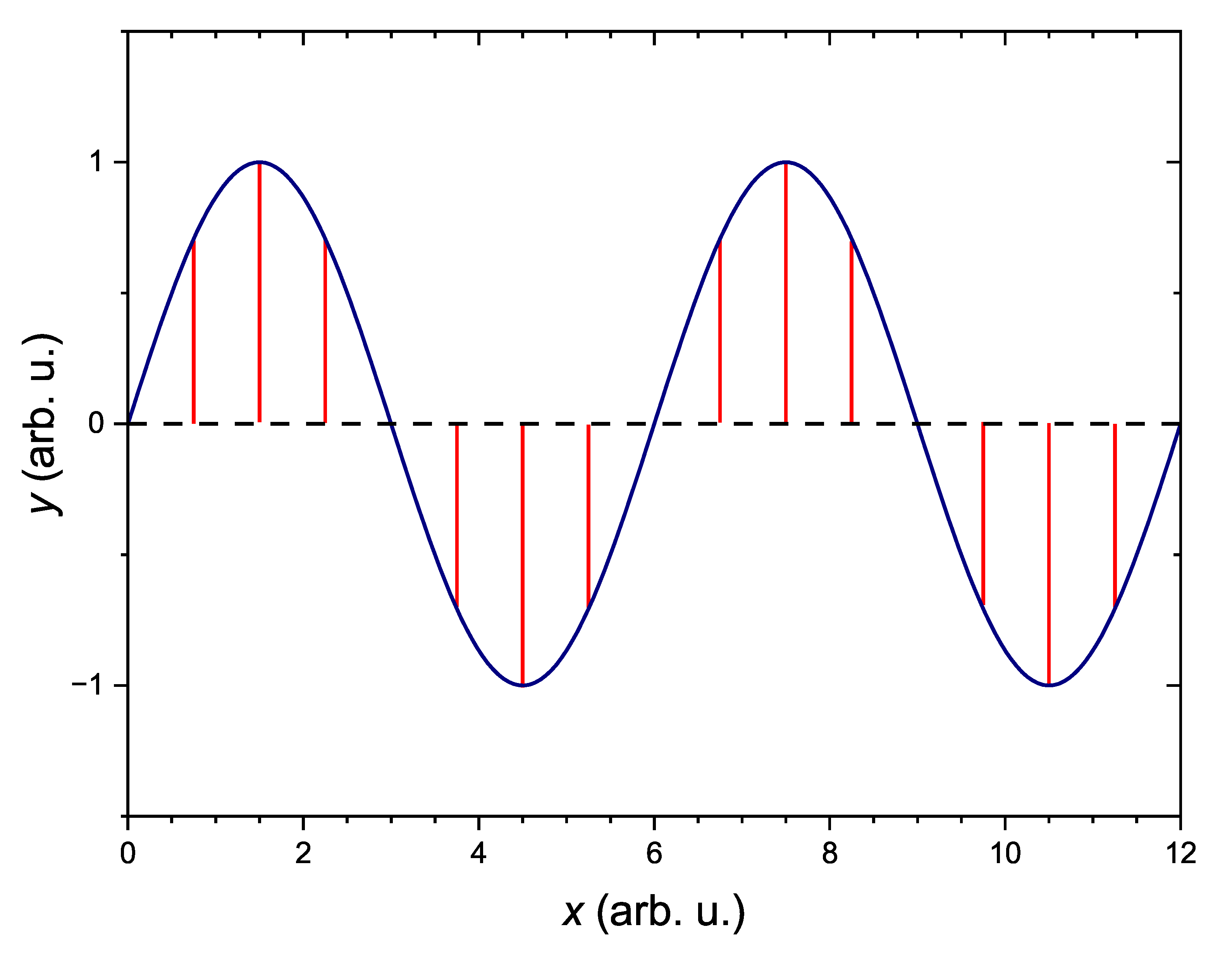
The blue line demonstrates the stretched string, and the red lines illustrate the attractive elastic interaction in
Figure 1.
By knowing these, we can specify the Lagrange function:
By applying Hamilton’s principle and performing variation along the fixed boundaries (such that only the “volume term” remains), we obtain the following Euler–Lagrange differential equation:
This equation is the well-known Klein–Gordon equation. By introducing the free propagation speed (without springs)
and the angular frequency
we can write the above equation in the following form:
Now, we consider an arrangement where the tiny springs pull the string points further away from the equilibrium position. This effect is equivalent to a repulsive interaction. In this case, the potential energy associated with the repulsive force field is
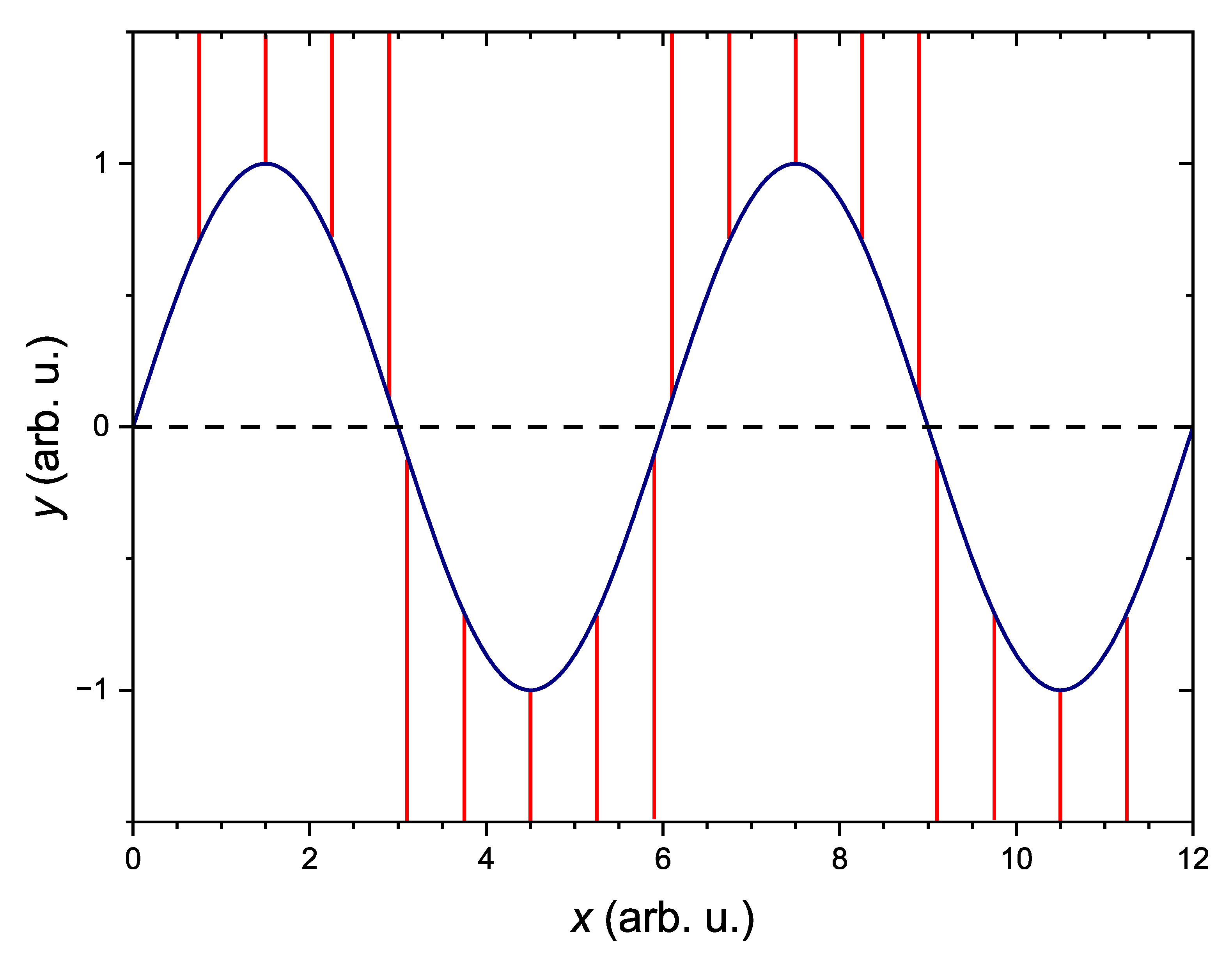
The blue line demonstrates the stretched string, and the red lines illustrate the repulsive elastic interaction in
Figure 2.
Then, the Euler–Lagrange equation becomes the following:
This repulsive interaction (by the
springs) cannot be realized technically. However, we can achieve an equivalent effect by imagining the traveling wave on a circular surface. If the angular velocity of the rotating disc is
, then the potential energy associated with the centrifugal force is a good approximation:
By applying this potential, the form of the Lagrange function is
Finally, we can derive the equation of motion as a Euler–Lagrange equation:
which is a “tachyon” Klein–Gordon equation controlled by the introduced repulsive interaction [
11]. The quotation marks indicate that this is not the case for a particle exceeding the speed of light. We apply the “tachyon” name due to the similarity of the mathematical equations and the structure of the related solutions.
2.2. Dynamic Transition
We focus on the dynamic consequences of the equation, including the repulsive effect. For this, by applying the canonical calculus [
17], we can express the momentum of the wave as
through which the Hamilton function is
The Hamiltonian is conserved. If we consider a part of a harmonic wave
with a finite length of
L (
is the amplitude,
k is the wave number, and
is the angular frequency), then we can calculate the Hamiltonian (entire energy) of a wave packet:
From here, the amplitude of
can be expressed:
When the angular velocity of the rotation reaches the value
then the amplitude will be unlimited:
The repulsive effect overcomes the attraction associated with the tension force.
If the angular velocity of
is small enough, then the string vibrates around its equilibrium position. However, above a certain threshold angular velocity, the string stretches to an increasingly large extension without oscillation due to the centrifugal force. This is the point when the dynamics alter. We can therefore find a critical angular velocity value below which all points of the string oscillate as a mode of wave propagation and above which the points of the string do not vibrate. This is a transition between the vibrational and the dissipative state (i.e., a dynamic phase transition). We can examine the above statement in detail with the help of dispersion relations:
We can express the phase velocity of the wave formed on a string with the formula
The wavelength does not alter. The angular frequency of
and the phase velocity of
decrease and tend toward zero with the increase in the angular velocity of
. The amplitude of
of the initial wave changes to
during the transition. This is due to the conservation of mechanical energy.
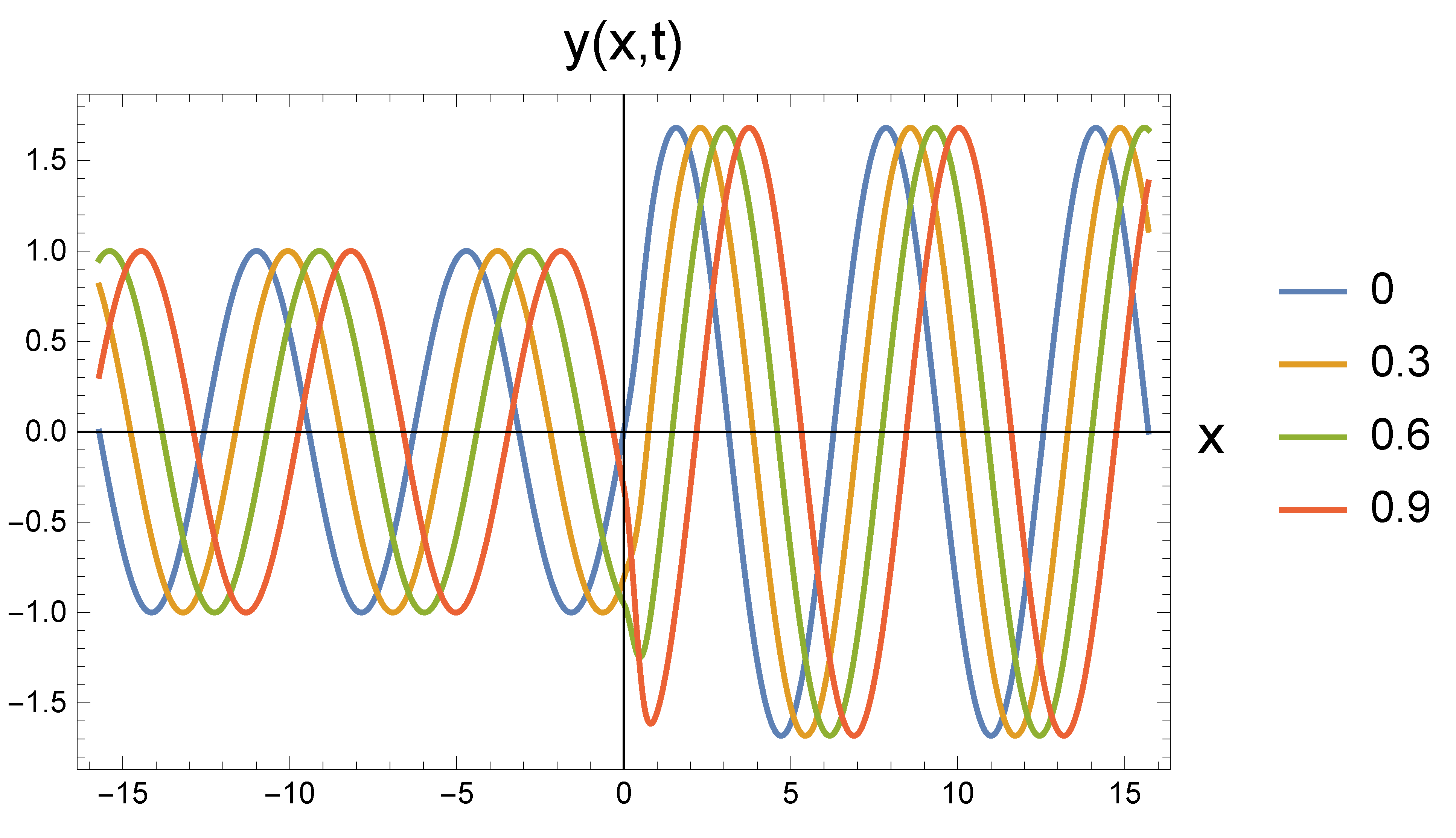
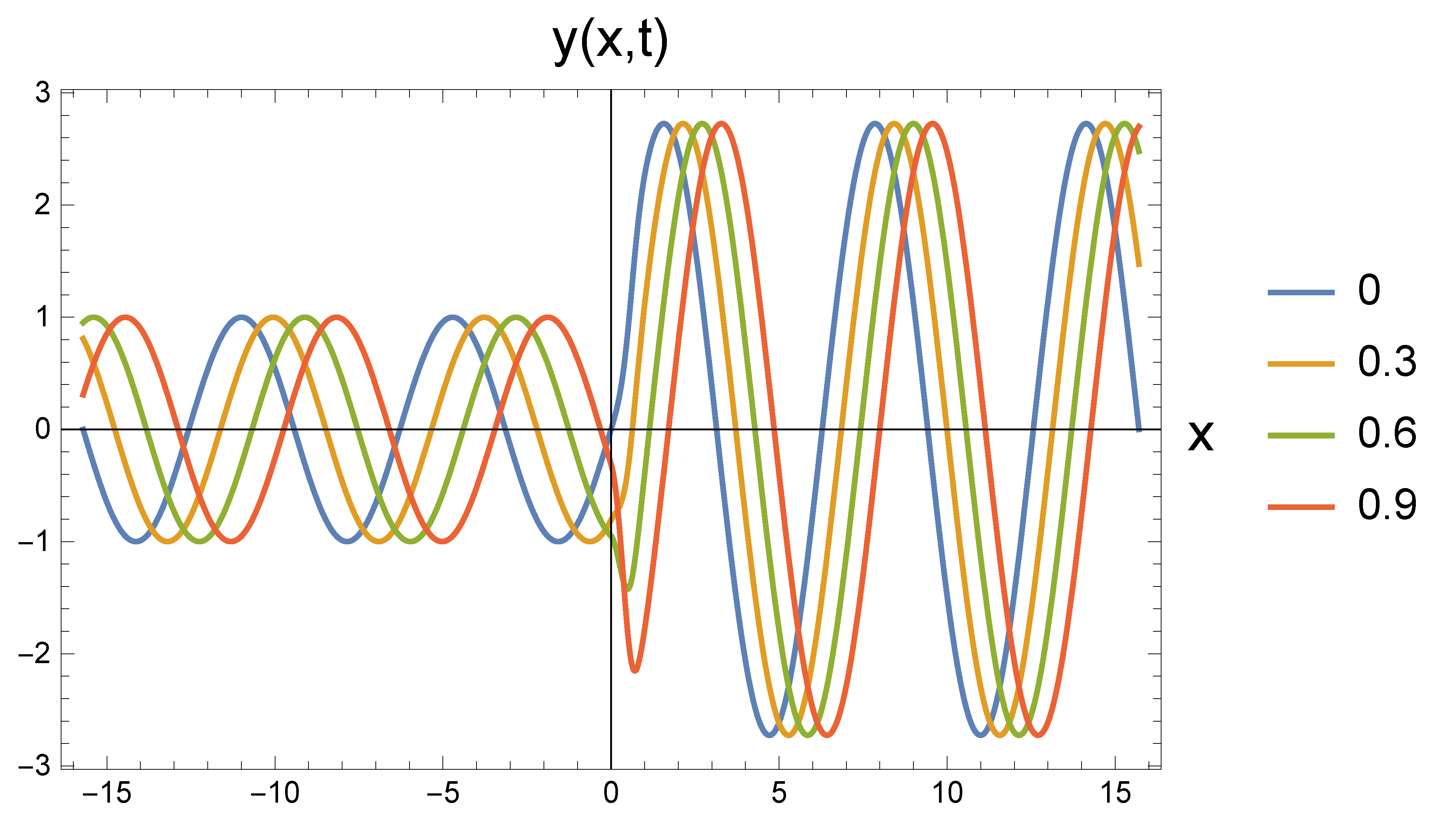
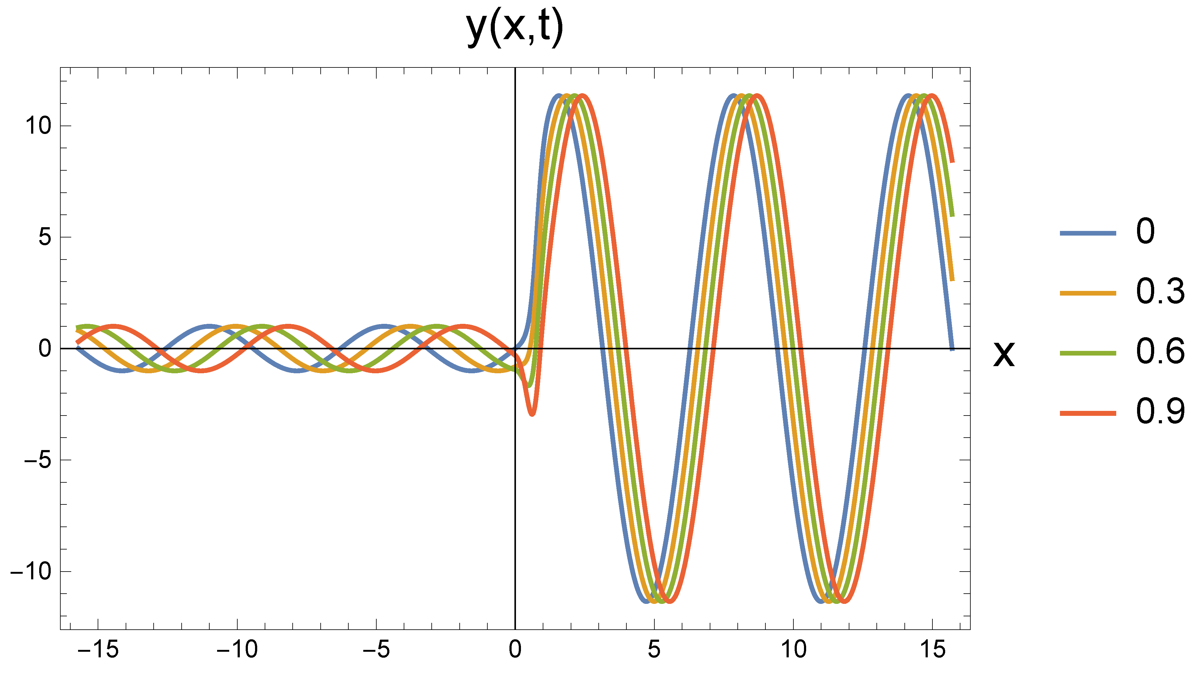
Figure 3,
Figure 4 and
Figure 5 clearly show that, in contrast to the angular frequency and amplitude, the wavelength did not change. A change in the angular frequency led to a decrease in the wave propagation speed near the critical point. This is the phenomenon of the critical value slowing down [
18] in the dynamic transitions. With the present parameterization, the dynamics change
(in natural units) occurred at this value. At that time, and for the subsequent
values, the deflection in the y direction in the repulsive potential space followed the exponentially increasing function sequence
The complex solution of displays this. There was no wave propagation in the x direction and only exponential decay in the y direction. This resulted from a change in the symmetry of the system. A crucial consequence was that the ordered wave propagation passed into an irreversible spreading motion in the y direction. This dispersion was related to the dissipation and had an immediate connection with the concept of irreversibility. The repulsive potential embodying a negative mass term was the source of the symmetry violation.
The authors currently do not know any mechanical experiments confirming the results of the presented calculations, but their reality is acceptable. It is easy to achieve a high angular velocity in small (microscopic) systems. However, wave propagation measurement can be problematic. In large-scale (m- or km-scale) systems, detecting wave propagation is not a problem, but a high angular velocity is.
3. The Negative Mass Term Thermal Klein–Gordon Equation
The second example of the Klein–Gordon equation with a negative mass term can be found in the thermal propagation [
12]. Here, we assume that the classical Fourier equation is the limiting case of a Lorentz invariant equation. Therefore, we formulate such an equation, which includes the repulsive effect condition. However, with this step, we shift directly to the K-G equation with a negative mass term.
3.1. Equations of Motion
To study thermal phenomena, let us start from the classical Fourier heat conduction equation:
This is such slow energy transport that we do not require the finite propagation speed of the physical action. This means that the propagation speed of the physical action (the action) is infinite. This should not be confused with the fact that heat propagation itself is a slow process. Here,
is the classical (local equilibrium) temperature,
is the heat conductivity coefficient, and
is the specific heat. It is known that if the equation of motion contains a first derivative, then the Lagrange function cannot be specified directly using the given variable [
16]. For this reason, we introduce a suitable potential function of
capable of generating the temperature field:
With the help of this, the expression of the Lagrange function can already be obtained:
After substituting the definition in Equation (
28) into the Euler–Lagrange equation calculated for
, we arrive at the Fourier heat propagation in Equation (
26).
If we want to describe fast energy transport, then we cannot ignore the limitation that at most, the effect can spread with the propagation speed of light of
c according to the theory of special relativity. In the case of such processes, we must interpret a so-called dynamic temperature of
, which is also defined by
, a Lorentz-invariant scalar field, and which also produces a Lorentz-invariant thermal field:
The equation describing such a fast process must be relativistically invariant. In this case, let the following be the Lagrangian density function:
Considering the above relationship between the potential and temperature, we obtain the equation describing the thermal field:
By substituting
this expression is the exact equivalent of Equation (
13):
Of course, here, c denotes the speed of light. Since this is a relativistically invariant equation, it does indeed have a tachyon solution.
3.2. Dispersion Relations, Symmetry Breaking, Dynamic Transition, and Classical Limits
The Lorentz-invariant equation must include the Fourier solution as a classical limiting case. However, we cannot drive this limit from a simple comparison of these equations. Differential equations cannot be reduced by omitting or reinterpreting individual terms. We can make the comparison at the level of dispersion relations. This is why we need to examine them.
The dispersion relations are obtained through a Fourier transformation of Equations (
26) and (
31) in order:
and
Here,
is the angular frequency, while
k is the wave number. By introducing the diffusivity parameter
, the group velocity corresponding to Equation (
35) is
If we move toward infinity with the speed of light, then the relation in Equation (
36) leads to
, which is the classical group velocity if we apply the
differentiation for the expression in Equation (
34). Therefore, the limiting case of the process (described by Equation (
31)) is the well-known Fourier thermal conduction. Furthermore, we know that Equation (
31) belongs to a non-dissipative process, and it has a wave solution. Now that we see the relationship between the two thermal propagations, for deeper insight, let us calculate the phase velocity from Equation (
35):
Let us introduce the
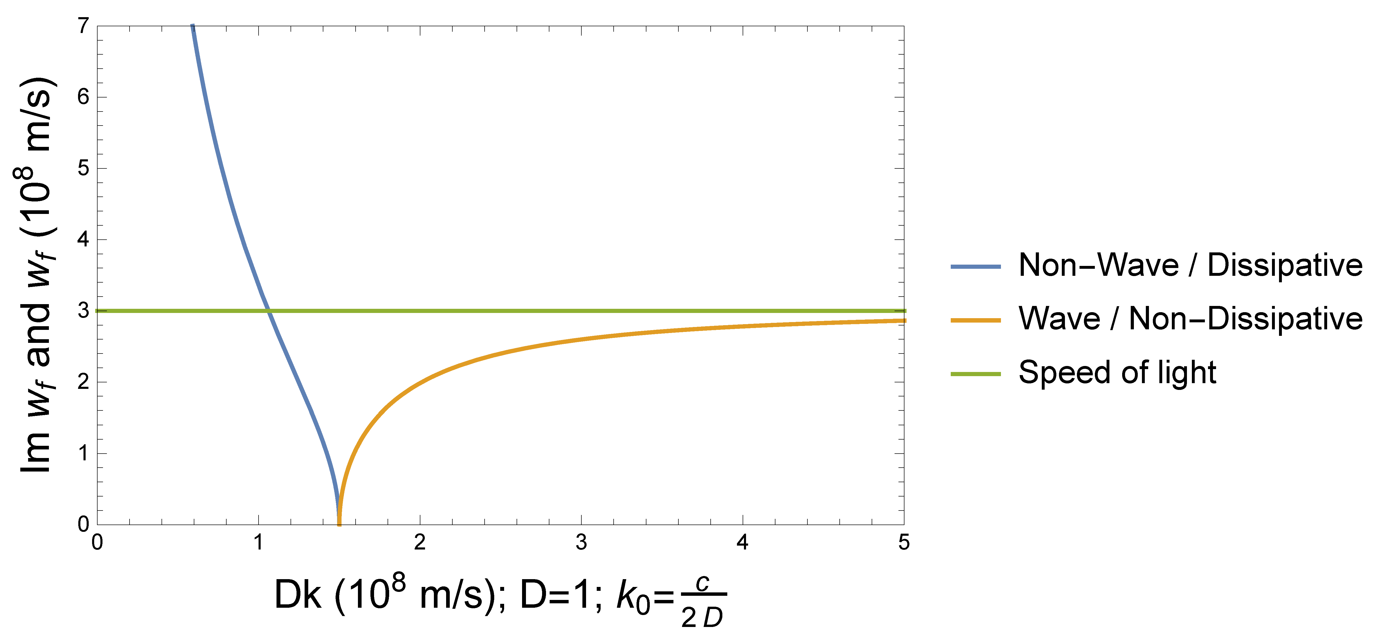
notation. We can see in
Figure 6 that if
, then
is real and a wave solution. If
, then
is imaginary and a non-wave solution. This is the breaking point of symmetry in the thermal process. We plotted
and
as a function of
, and we can see that the critical slowdown [
18] occurred in the vicinity of the value of
. This change in dynamics fully corresponds to what we experienced in the case of the presented mechanical wave. Thus, we can say that the appearance of motion equations with a negative mass term is natural in two major physical disciplines.
Let us return to Equation (
35) for a brief quantitative discussion. If
then non-dissipative wave propagation takes place. This means that the wavelength modes
propagate reversibly. The equality belongs to the symmetry breaking of the dynamics. Since the heat conduction coefficient is 2–3 orders of magnitude smaller for most materials, thermal conduction is always irreversible, according to past experience. Carbon nanotubes [
19,
20] can be said to be exceptional, for which
W/m·K (this may be an underestimated value) and
J/kg·K, with which
nm (i.e., these are phonons in the UV range). For larger
values [
21],
can reach up to 1000 nm. From a technical point of view, this can have many possibilities.
We see that the fit of the K-G equation with a negative mass term to the classical limit case (Fourier heat conduction) works well. However, using a Lorentz invariant thermal equation may be more likely to be relevant in field theories. One example is the coupling of the Friedmann equation and this space [
22].
3.3. Lagrangian Reloaded
The Lorentz invariant thermal Klein–Gordon equation formulated in Equation (
31) involves only self-adjoint operators (simply, there are no odd-order derivatives in the equation of motion), and thus we can express the Lagrange function using the physical variable temperature of
directly:
We do not forget here that the temperature T is for a more abstract physical field.
4. The Negative Mass Term Electrodynamic Klein–Gordon Equation
In the previous sections, we showed in the case of two classical physical fields that we naturally found a Klein–Gordon equation with a negative mass term. Now, we turn the thought process around a bit. We start from the assumption that there is also a K-G equation with a negative mass term in electrodynamics. The question is what we should change in Maxwell’s equations to achieve this goal. This concern raises whether such a step is possible at all. We conduct a calculation experiment for now, and we can say more once we know the final result.
4.1. Introducing a Repulsive Interaction in the Electromagnetism
Inspired by the previous two examples, the question arises of whether there is a Klein–Gordon equation with a negative mass term in the case of electrodynamics. To answer this, let us start from the well-known form of Maxwell’s equations [
23]:
By applying these relations, we can deduce the usual wave equations with the relevant source terms on the right-hand side of the expressions:
What effect do we assume exists to answer the above question? We add a term
to the right side of Equation (
42). Here, the parameter of
refers to the hypothesized interaction. Then, the modified form of Maxwell’s equation is
To solve the equations, we introduce the vector potential of
with the usual relation
and the scalar potential of
, which take into account the modified form in the electric field:
By considering the Lorenz condition
and applying the relation
, we arrive at the equation
Learning from Equations (
13) and (
33), we can identify
. With the third (negative) term, the K-G equation in Equation (
50) involves a repulsive potential. The structure of the equation is similar to that of the equations discussed in the previous chapters, and thus it contains a dynamic phase transition depending on the parameter of
. An equation with a similar structure can be derived for the vector potential of
as well as for the fields of
and
[
15]:
In this way, the desired equations appear for the potential fields of
and
. At the same time, we also obtain equations that are similar in structure to measurable physical fields:
4.2. Spontaneous Peak Effect
The subject of our further investigation is what kind of physical dynamics the obtained equations describe. Let us start with the following assumption. Initially, we imagined an electrically conductive field with zero for the charge density. This means the electric charges can move freely if even a weak disturbance affects the considered medium. We assumed a small perturbation of a Gaussian charge distribution. Now, we can examine the appearing electrical field dynamics given by Equation (
52). Here, we can eliminate the last two terms of this equation to simplify the problem to
We remark that it has been shown that the contribution of the current and its time derivative result in a value of zero [
15]. We can solve this equation by applying the Green function method, and thus the evolution of the electric field of
can be expressed from an initial charge distribution of
:
The expression in
is the Green function
. (The integration runs in the four-dimensional spacetime.) The calculated Green function for the present physical dynamics is called the Wheeler propagator
[
24,
25]. The effect of the Wheeler propagator is generation of the electric state
at a later time
t from the initial charge density at time
.
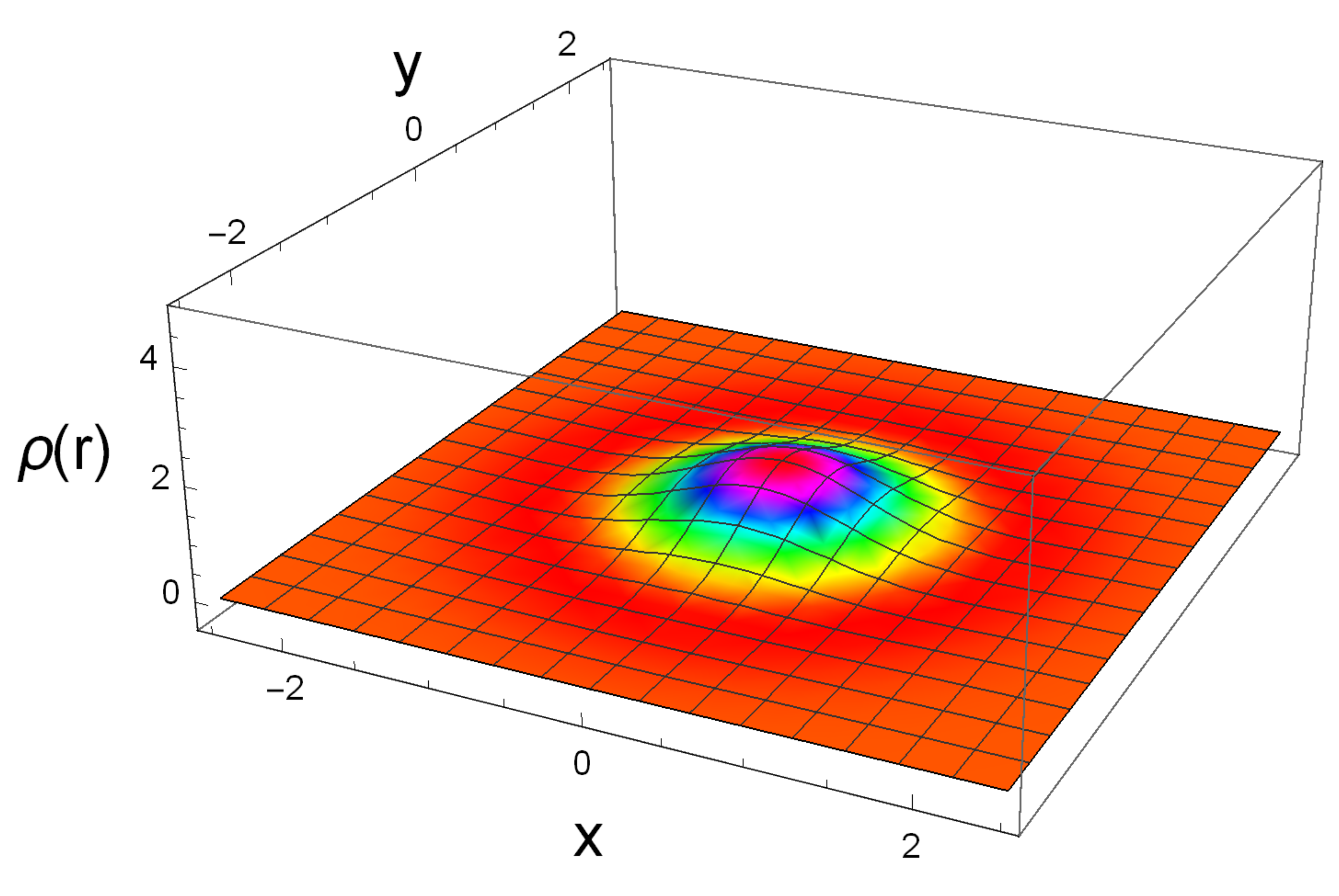
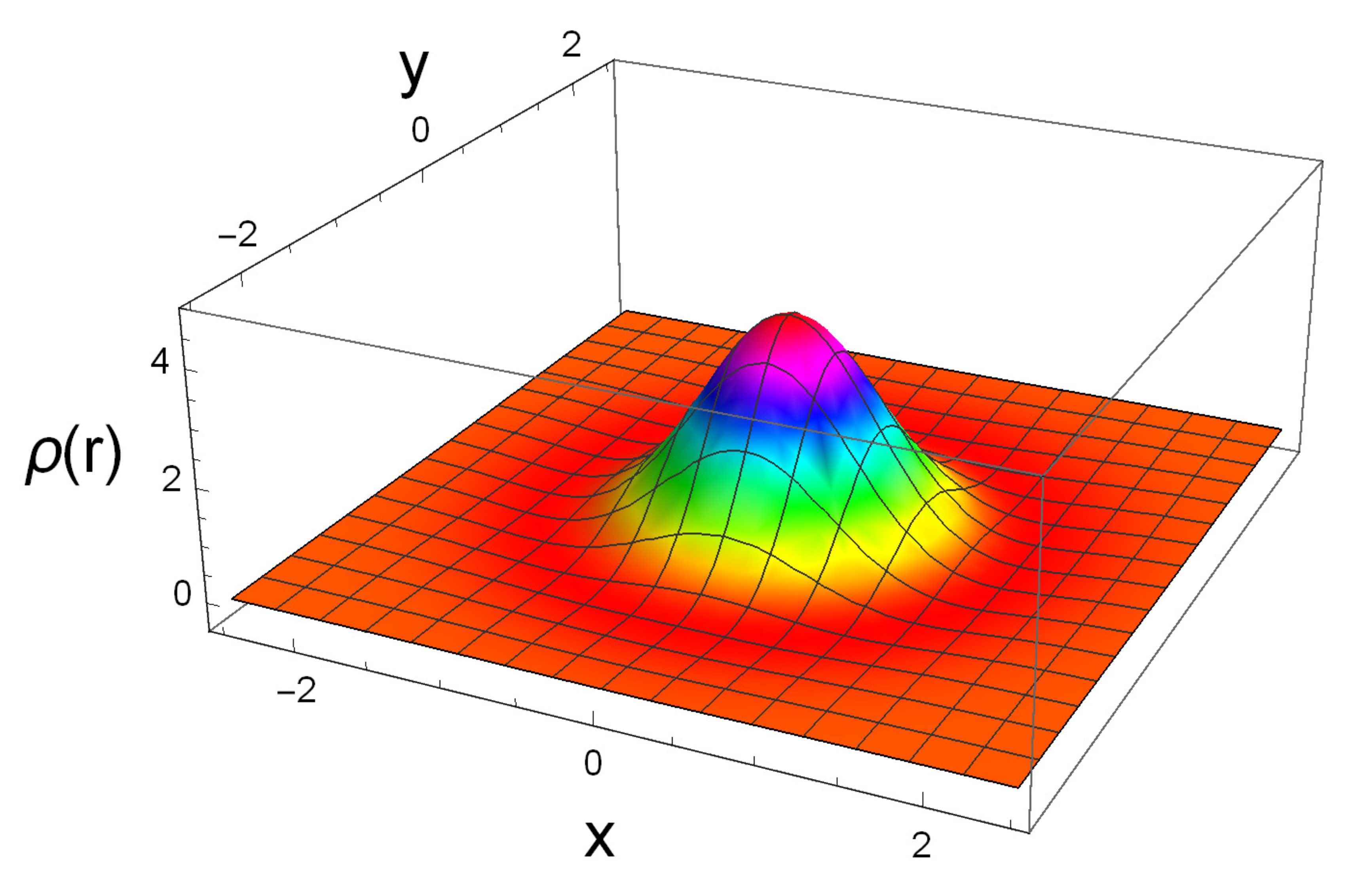
Figure 7,
Figure 8 and
Figure 9 show the distribution of the charge density peaks at different moments in time.
4.3. Simplified Electric Potential (Charge and Electric Current Density) Vector Potential Relations
We can find the relationship between the spontaneous charge density and the electric potential, and similarly the relationship between the associated current density and the vector potential from Equations (
50) and (
51), in two simple equations:
and
The meaning of the equations can be considered trivial in a physical sense. In the next section, we primarily need the relationship between the charge density and the electric potential.
5. Charge Density Oscillations
The previous three examples discussed cases of repulsive interaction. The amplitude of the oscillation increased in the mechanical example in
Section 2, the temperature spread in the thermal case in
Section 3, and a charge peak formed in the electromagnetism in
Section 4. However, the electromagnetic charge density peak, being the charge separation caused by the repulsive electromagnetic effect, cannot be unlimited. The Coulomb attractive effect plays an essential role in this.
We can define a characteristic wavelength of
for the movement of charged particles from the vibration of
under the influence of electromagnetic repulsion in Equations (
56) and (
57):
The movement of charged particles depends on their mass. We may assume that the mass
m consists of
N electrons expressed by
. Then, we can derive the charge density in Equation (
56) for this set of particles:
The resulting vibration indicates the separation of
N positively and
N negatively charged particles. The Coulomb potential perceptible to electrons from a set of positively charged particles
is
where
r is the distance between the charged entities and
e is the elementary charge. One packet of the particles (e.g., the positive charges) has the charge density
. We may assume a sphere-like symmetric distribution, and thus the integral can be applied for the potential-charge density relation in Equation (
59):
where
a is the maximal extension of the charged packet. By substituting the right-hand side of Equation (
59), we obtain
We compare Equations (
61) and (
62), from which we obtain a relation for the maximal displacement of
a as a function of the charged particles:
The maximal distance of the spontaneous charge distinction may be in the case of
. If the characteristic wavelength of
we introduced is identified with the Compton wavelength of
m as a typical value on this scale, then we obtain
m. The minimal time period is
s. The related (maximal) angular frequency is
1/s, which almost equals the angular frequency of the Zitterbewegung
1/s [
26,
27,
28]. The Zitterbewegung effect has been experimentally verified [
29,
30,
31]. It can also be seen that the chance of creating a large number of particle groups decreases with the reciprocal of N.
This phenomenon perhaps justifies the term added to Maxwell’s equation, which creates the repulsive effect. We are sure that the K-G equation with a negative mass term is part of all three classical disciplines, and we can assign an acceptable physical meaning to all three. At the same time, a similar change in dynamics and a breaking of the internal symmetry appear in all three. This may not be just a coincidence after all.
6. Conclusions
In the present article, we dealt with the appearance of Klein–Gordon equations with a negative mass term in different physical problems. In all three classical disciplines, we showed how it appears, what kind of interpretation pertains to the equations, and what dynamic changes and symmetry violations hide in the background. In the different sections, we discussed the phenomena one by one. In mechanics, the K-G equation with a positive mass term is well known concerning wave propagation. Here, in addition to the force stretching the string, one only has to imagine the existence of a transverse force field in an elastic medium. Our idea is to replace the attractive, flexible space with a repulsive one. The experimental proof is not easy in an elastic environment. However, if we imagine that the elastic wave travels on a rotating disc, the centrifugal potential corresponds to a repulsive effect. At the level of the equations, only one sign change takes place, but the effect is undoubtedly significant. For the dynamics of wave propagation change, instead of vibration modes, in the vertical (y) direction, an exponentially time-dependent movement appears. At the same time, the velocity of the wave in the horizontal (x) direction tends toward zero. These new results were plotted on graphs, and the phenomenon of critical slowdown was visible. This is one of the most characteristic features of critical dynamic phenomena. The description of thermal propagation is the second major topic of the present paper. Against the previous mechanical phenomenon, the “slowed down” process is known as Fourier heat conduction. The task was to show the equation from which we could derive it, taking into account the finite propagation speed of the effect. To fulfill these requirements, we created a Lorentz-invariant Lagrange function, which led to a similarly Lorentz-invariant equation of motion. This equation is a K-G equation with a negative mass term. After that, we showed through the dispersion relations that the description given in this way led to classical heat conduction in the limiting case . The change in dynamics can be followed in the wave vs. non-wave transition consistently at the level of the parameters. We could identify the phenomenon of critical slowdown. Thermal wave propagation may exist under certain conditions, and the possibility of reversible behavior of nanoscale thermal processes also arises. We feel a sense of loss, wondering what the situation is in electrodynamics. The examples of mechanics and thermodynamics inspired us to believe that in this case too, there must be a K-G equation with a negative mass term. Although there is no experimental proof of this motion, it is still worth trying to find the related mathematical construction. For this purpose, we added a term to the equation involving Faraday’s law of induction. We emphasize that this is only a mathematical assumption. The equations derived for the quantities describing the electromagnetic fields in this way are all K-G equations with a negative mass term. The effect of this term in the theory is that it causes a spontaneous charge peak in the initially homogeneous zero charge density distribution. The Coulomb interaction is against the charge separation. The two physical effects may cause a high-frequency vibration that may appear as a combination of the two effects.
To summarize, we can say that those phenomena governed by K-G equations with negative mass terms involve repulsive interactions. Consequently, these interactions change the dynamics of the physical processes, which in this nature are not unusual. The similarity of the equations suggests that on the one hand, the coupling of the phenomena is possible at this mathematical level, and on the other hand, the phenomenon of dissipation may be an integral part of the theory.
Author Contributions
The authors contributed equally to this work. Conceptualization, F.M. and K.G.; methodology, F.M. and K.G; validation, K.G.; visualization, F.M.; writing—original draft, F.M. and K.G. All authors have read and agreed to the published version of the manuscript.
Funding
This research was supported by the National Research, Development and Innovation Office (NKFIH) (grant no. K137852) and by the Ministry of Innovation and Technology and NKFIH within the Quantum Information National Laboratory of Hungary. Supported by the V4-Japan Joint Research Program (BGapEng), financed by the National Research, Development and Innovation Office (NKFIH) under grant no. 2019-2.1.7-ERA-NET-2021-00028. Project no. TKP2021-NVA-16 was implemented with the support provided by the Ministry of Innovation and Technology of Hungary from the National Research, Development and Innovation Fund.
Data Availability Statement
Data are contained within the article.
Conflicts of Interest
The authors declare no conflicts of interest.
References
- Wess, J.; Zumino, B. Supergage Transformations in Four Dimensions. Nucl. Phys. B 1974, 70, 39. [Google Scholar] [CrossRef]
- Wess, J.; Zumino, B. Supergage Invariant Extension of Quantum Electrodynamics. Nucl. Phys. B 1974, 78, 1. [Google Scholar] [CrossRef]
- Bollini, C.G.; Giambiagi, J.J. Generalized Klein-Gordon equations in d dimensions from supersymmetry. Phys. Rev. D 1985, 32, 3316. [Google Scholar] [CrossRef]
- Recami, E. Classical Tachyons and Possible Applications. Riv. Nuovo Cimento 1986, 9, 1. [Google Scholar] [CrossRef]
- Sommerfeld, A. Simplified Deduction of the Field and the Forces of an Electron Moving in Any Given Way. K. Akad. Wet. Amst. Proc. 1904, 7, 345. [Google Scholar]
- Bilaniuk, O.M.P.; Deshpande, V.K.; Sudarshan, E.C.G. “Meta” Relativity. Am. J. Phys. 1962, 30, 718. [Google Scholar] [CrossRef]
- Feinberg, G. Possibility of Faster-Than-Light Particles. Phys. Rev. 1967, 159, 1089. [Google Scholar] [CrossRef]
- Agudin, J.L.; Platzeck, A.M. Tachyons and the Radiation of an Accelerated Charge. Phys. Rev. D 1982, 26, 1923. [Google Scholar] [CrossRef]
- Barci, D.G.; Bollini, C.G.; Rocca, M. The Tachyon Propagator. II Nuovo C. A 1993, 106, 603. [Google Scholar] [CrossRef][Green Version]
- Barci, D.G.; Bollini, C.G.; Oxman, L.E.; Rocca, M. Higher Order Equations and Constituent Fields. Int. J. Mod. Phys. A 1994, 23, 4169. [Google Scholar] [CrossRef]
- Gambár, K.; Márkus, F. A Simple Mechanical Model to Demonstrate a Dynamical Phase Transition. Rep. Math. Phys. 2008, 62, 219. [Google Scholar] [CrossRef]
- Márkus, F.; Gambár, K. Wheeler Propagator of the Lorentz Invariant Thermal Energy Propagation. Int. J. Theor. Phys. 2010, 49, 2065. [Google Scholar] [CrossRef]
- Ma, S.-K. Modern Theory of Critical Phenomena; Addison-Wesley: Redwood City, CA, USA, 1982. [Google Scholar]
- Wei, C.; Li, A. Existence and multiplicity of solutions for Klein–Gordon–Maxwell systems with sign-changing potentials. Adv. Diff. Eq. 2019, 72. [Google Scholar] [CrossRef]
- Gambár, K.; Rocca, M.C.; Márkus, F. A Repulsive Interaction in Classical Electrodynamics. Acta Polytechn. Hung. 2020, 17, 175. [Google Scholar] [CrossRef]
- Morse, P.M.; Feshbach, H. Methods of Theoretical Physics; McGraw-Hill: New York, NY, USA, 1953. [Google Scholar]
- Courant, R.; Hilbert, D. Methods of Mathematical Physics; Interscience: New York, NY, USA, 1966. [Google Scholar]
- Scheffer, M.; Carpenter, S.R.; Lenton, T.M.; Bascompte, J.; Brock, W.; Dakos, V.; van de Koppel, J.; van de Leemput, I.A.; Levin, S.A.; van Nes, E.H.; et al. Anticipating Critical Transitions. Science 2012, 338, 344. [Google Scholar] [CrossRef] [PubMed]
- Berber, S.; Kwon, Y.-K.; Tománek, D. Unusually High Thermal Conductivity of Carbon Nanotubes. Phys. Rev. Lett. 2000, 84, 4613. [Google Scholar] [CrossRef]
- Cao, J.X.; Yan, X.H.; Xiao, Y. Specific heat of Single-Walled Carbon Nanotubes: A Lattice Dynamics Study. J. Phys. Soc. Jpn. 2003, 72, 2256. [Google Scholar] [CrossRef]
- Cao, J.X.; Yan, X.H.; Xiao, Y.; Ding, J.W. Thermal Conductivity of Zigzag Single-Walled Carbon Nanotubes: Role of the Umklapp Process. Phys. Rev. B 2004, 69, 073407. [Google Scholar] [CrossRef]
- Márkus, F.; Vázquez, F.; Gambár, K. Time Evolution of Thermodynamic Temperature in the Early Stage of Universe. Phys. A Stat. Mech. Appl. 2009, 388, 2122. [Google Scholar] [CrossRef]
- Jackson, J.D. Classical Electrodynamics; John Wiley & Sons: Hoboken, NJ, USA, 1999. [Google Scholar]
- Bollini, C.G.; Rocca, M.C. Wheeler Propagator. Int. J. Theor. Phys. 1998, 37, 2877. [Google Scholar] [CrossRef]
- Bollini, C.G.; Oxman, L.E.; Rocca, M.C. Coupling of Tachyons to Electromagnetism. Int. J. Theor. Phys. 1999, 38, 777. [Google Scholar] [CrossRef]
- Breit, G. An Interpretation of Dirac’s Theory of the Electron. Proc. Nat. Acad. Sci. USA 1928, 14, 553. [Google Scholar] [CrossRef] [PubMed]
- Schrödinger, E. Über die kräftefreie Bewegung in der relativistischen Quantenmechanik. Sitzungsber. Preuss. Akad. Wiss. Phys. Math. Kl. 1930, 24, 418. (In German) [Google Scholar]
- Roy, C.L.; Basu, C.; Roy, A. On the Derivation of Zitterbewegung. Phys. Lett. A 1989, 137, 319. [Google Scholar] [CrossRef]
- Wang, Y.-X.; Yang, Z.; Xiong, S.-J. Study of Zitterbewegung in Graphene Bilayer with Perpendicular Magnetic Field. Europhys. Lett. 2010, 89, 17007. [Google Scholar] [CrossRef]
- LeBlanc, L.J.; Beeler, M.C.; Jiménez-García, K.; Perry, A.R.; Sugawa, S.; Williams, R.A.; Spielman, I.B. Direct Observation of Zitterbewegung in a Bose–Einstein Condensate. New J. Phys. 2013, 15, 073011. [Google Scholar] [CrossRef]
- Lovett, S.; Walker, P.M.; Osipov, A.; Yulin, A.; Naik, P.O.; Whittaker, C.E.; Shelykh, I.A.; Skolnick, M.S.; Krizhanovskii, D.N. Observation of Zitterbewegung in Photonic Microcavities. Light Sci. Appl. 2023, 12, 126. [Google Scholar] [CrossRef]
Figure 1.
Mechanical Klein–Gordon wave propagation, with a string of density stretched by a force F. The red lines demonstrate the attractive linear force field. This force field is proportional to the vertical displacement . This is the “extra” interaction compared with the usual transverse wave.
Figure 1.
Mechanical Klein–Gordon wave propagation, with a string of density stretched by a force F. The red lines demonstrate the attractive linear force field. This force field is proportional to the vertical displacement . This is the “extra” interaction compared with the usual transverse wave.
Figure 2.
Mechanical Klein–Gordon wave propagation, with a string of a density stretched by a force F. The red lines demonstrate the repulsive linear force field. This force is proportional to the vertical displacement .
Figure 2.
Mechanical Klein–Gordon wave propagation, with a string of a density stretched by a force F. The red lines demonstrate the repulsive linear force field. This force is proportional to the vertical displacement .
Figure 3.
Wave transition between force-free and repulsive potential field. The latter is implemented with a rotating disk with an angular velocity of in natural units.
Figure 3.
Wave transition between force-free and repulsive potential field. The latter is implemented with a rotating disk with an angular velocity of in natural units.
Figure 4.
Wave transition between force-free and repulsive potential field. The latter is implemented with a rotating disk with an angular velocity of in natural units.
Figure 4.
Wave transition between force-free and repulsive potential field. The latter is implemented with a rotating disk with an angular velocity of in natural units.
Figure 5.
Wave transition between force-free and repulsive potential field. The latter is implemented with a rotating disk with an angular velocity of in natural units.
Figure 5.
Wave transition between force-free and repulsive potential field. The latter is implemented with a rotating disk with an angular velocity of in natural units.
Figure 6.
Dynamic transition between non-wave (dissipative) and wave-like (non-dissipative) propagation. The critical transition point is at . The diffusivity parameter is D = 1. The phase velocity of of the wave-like propagation is always less than the speed of light.
Figure 6.
Dynamic transition between non-wave (dissipative) and wave-like (non-dissipative) propagation. The critical transition point is at . The diffusivity parameter is D = 1. The phase velocity of of the wave-like propagation is always less than the speed of light.
Figure 7.
A 2D plot of the charge density as a function of the radius over time, where . Red color means zero charge density. The colors red, yellow, green, blue, and magenta, in that order, show the increasing charge density. The charge density and radius are understood in natural units.
Figure 7.
A 2D plot of the charge density as a function of the radius over time, where . Red color means zero charge density. The colors red, yellow, green, blue, and magenta, in that order, show the increasing charge density. The charge density and radius are understood in natural units.
Figure 8.
A 2D plot of the charge density as a function of the radius over time, where . Red color means zero charge density. The colors red, yellow, green, blue, and magenta, in that order, show the increasing charge density. The charge density and radius are understood in natural units.
Figure 8.
A 2D plot of the charge density as a function of the radius over time, where . Red color means zero charge density. The colors red, yellow, green, blue, and magenta, in that order, show the increasing charge density. The charge density and radius are understood in natural units.
Figure 9.
A 2D plot of the charge density as a function of the radius over time, where . Red color means zero charge density. The colors red, yellow, green, blue, and magenta, in that order, show the increasing charge density. The charge density and radius are understood in natural units.
Figure 9.
A 2D plot of the charge density as a function of the radius over time, where . Red color means zero charge density. The colors red, yellow, green, blue, and magenta, in that order, show the increasing charge density. The charge density and radius are understood in natural units.
| Disclaimer/Publisher’s Note: The statements, opinions and data contained in all publications are solely those of the individual author(s) and contributor(s) and not of MDPI and/or the editor(s). MDPI and/or the editor(s) disclaim responsibility for any injury to people or property resulting from any ideas, methods, instructions or products referred to in the content. |
© 2024 by the authors. Licensee MDPI, Basel, Switzerland. This article is an open access article distributed under the terms and conditions of the Creative Commons Attribution (CC BY) license (https://creativecommons.org/licenses/by/4.0/).


