Detecting Phase Transitions through Non-Equilibrium Work Fluctuations

Abstract

We show how averages of exponential functions of path-dependent quantities, such as those of Work Fluctuation Theorems, detect phase transitions in deterministic and stochastic systems. State space truncation—the restriction of the observations to a subset of state space with prescribed probability—is introduced to obtain that result. Two stochastic processes undergoing first-order phase transitions are analyzed both analytically and numerically: a variant of the Ehrenfest urn model and the 2D Ising model subject to a magnetic field. In the presence of phase transitions, we prove that even minimal state space truncation makes averages of exponentials of path-dependent variables sensibly deviate from full state space values. Specifically, in the case of discontinuous phase transitions, this approach is strikingly effective in locating the transition value of the control parameter. As this approach works even with variables different from those of fluctuation theorems, it provides a new recipe to identify order parameters in the study of non-equilibrium phase transitions, profiting from the often incomplete statistics that are available.

1. Introduction

Exponentials of microscopically expressed variables have been used for a long time in statistical physics and molecular dynamics. Bennett’s formulae for the free energy [1], Widom’s relation [2], and Zwanzig’s relation [3], are among them. More recently, they have become popular in non-equilibrium statistical mechanics in the form of Fluctuation Relations [4,5,6], which constitute a step in the direction of generalizing linear response theory and the Fluctuation Dissipation Relation, and in the form of Work Fluctuation Theorems (WFT) [7,8,9,10], which focus on equilibrium properties derived from non-equilibrium processes. See [11,12] for comprehensive reviews and [13,14,15,16,17,18,19,20,21,22,23,24,25] for further discussion.

Exponential observables, such as $e^{-\mathit{\beta }\mathit{\sigma }}$, with $\mathit{\sigma }$ denoting a kind of dissipation functional of the system trajectories, may provide useful insight into the properties of non-equilibrium systems but need to be handled with care. At the very least, the amount of data for accurate calculations may be prohibitively large because substantial contributions to the statistical properties of such observables pertain to the (low probability) tails of the relevant distributions, e.g., [7]. The problem is often enhanced by high energy barriers that keep trajectories from accessing specific regions. The problem is well known. For instance, in the context of free energy differences estimation [1,26], numerous ad hoc techniques and procedures have been developed to deal with it [27,28,29]. In general, many challenges remain. Moreover, the recent work [30], concerning the canonical ensemble of classical Hamiltonian systems shows how exponential variables can be strongly affected by finite-size effects or lack of ergodicity [30]. This must be considered, in particular, when dealing with small systems because ensembles were originally conceived to treat specific observables of large systems that (a) are not affected by finite-size effects and (b) their time averages equal their phase space averages.

In this paper, we will show how the above difficulties can actually be leveraged to recover important information about the system behavior. This way, often unavoidable hindrances in the investigation of the objects of modern interest may turn profitable under some conditions.

We start by concisely recalling the theoretical background of WFT for Markov processes [31,32,33] and the notion of absolute irreversibility [34,35,36,37]. Then, we introduce the concepts of state space truncation, which can be interpreted both as a result of incomplete information on the system of interest, or as the representation of a system with finitely many degrees of freedom, interacting with only a portion of its environment. This is of interest, for instance, when the system is subjected to rapid transformations, which is common in present-day bio- and nano-technologies. We find that the corresponding ensemble averages of $e^{-\mathit{\beta }{W}_d}$, $W_d$ being the dissipated work, may detect phase transitions and locate them in parameter space.

This is shown by analyzing a variant of the celebrated Ehrenfest urn model in detail, derived from a deterministic 2D model of particle transport [38], and a classical 2D Ising model with periodic boundary conditions in a magnetic field. For both, it is found that the ensemble average of $e^{-\mathit{\beta }{W}_d}$ as a function of the driving control parameter, computed over trajectories starting in the lowest energy states (thus, with highest stationary probability), manifests a discontinuity in the thermodynamic limit whenever the system undergoes a first-order phase transition. A smooth dependence is instead found in the case of the Ising model at supercritical temperatures.

This paper is structured as follows: in Section 2 we introduce the theoretical background and the ensemble averages over relevant subsets of the state space, along with the notion of absolute irreversibility. Section 3 analyzes in detail the systems undergoing phase transitions mentioned above, using a suitably amended version of the Jarzynski Equality. Conclusions are drawn in Section 4.

2. Theory and Methods

2.1. Work and Free Energy for Markov Chains

Here, we concisely recall some basic concepts referring to discrete time Markov chains [39,40]. A Markov chain is a finite set of random variables $\mathbf{X}={\left(X_i\right)}_{i=0}^{\mathit{\tau }}$, with $\mathit{\tau }\in \mathbb{N}$, taking values on a finite state space S, such that

$$P\left(X_i=x_i|X_0=x_0,\dots ,X_{i-1}=x_{i-1}\right)=P\left(X_i=x_i|X_{i-1}=x_{i-1}\right)$$

for every $0<i\le \mathit{\tau }$ and every sequence $x_0,\dots ,x_{i-1}$ for which $P\left(X_0=x_0,\dots ,X_{i-1}=x_{i-1}\right)>0$. The elements of S correspond to the possible states of the system, with $X_i$ representing the state at time i. The transition matrix $Q=\left(Q_{xy}\right)$ has entries $Q_{xy}=P(X_i=y|X_{i-1}=x)$, for all $x,y\in S$ and $0<i\le \mathit{\tau }$, representing the transition probabilities from the state x to the state y, which obey ${\sum }_{y\in S}{Q}_{xy}=1$, for all $x\in S$. A specific realization of the sequence $X_0,\dots ,X_{\mathit{\tau }}$ is characterized by the probability of the path ${\mathcal{P}}_{{\mathit{\mu }}_0}\left(\mathbf{x}\right)={\mathit{\mu }}_0\left(x_0\right)\mathcal{P}\left(\mathbf{x}\right|x_0)={\mathit{\mu }}_0\left(x_0\right){\prod }_{i=0}^{\mathit{\tau }-1}{Q}_{x_i{x}_{i+1}}$, where ${\mathit{\mu }}_0\left(x\right)=P(X_0=x)$ is an assigned discrete probability distribution and $\mathbf{x}=(x_0,x_1,\dots ,x_{\mathit{\tau }})\in S^{\mathit{\tau }+1}$. We recall that a Markov chain admits a unique invariant distribution $\mathit{\mu }$ on S, such that $\mathit{\mu }Q=\mathit{\mu }$ (where $\mathit{\mu }$ is conceived as a row vector) if it is irreducible and its states are ergodic, i.e., they are aperiodic and persistent with a finite mean recurrence time [41]. An explicit time dependence is sometimes introduced in the definition of the transition matrices to mimic the effect of an external drive affecting the evolution of the system. The action of the drive is expressed by the protocol $\mathit{\lambda }\left(i\right)={\mathit{\lambda }}_i$, $i=0,1,\dots ,\mathit{\tau }$. This way, the Markov chain turns inhomogeneous, namely ${\left(Q_i\right)}_{xy}=P(X_i=y|X_{i-1}=x)$ depends on time. One may then introduce the following path-dependent quantity, called work [42]:

$$W=\sum _{i=0}^{\mathit{\tau }-1}\left[E_{i+1}\left(x_i\right)-E_i\left(x_i\right)\right]$$

where the function $E_i\left(x_i\right)$ is related to a distribution ${\mathit{\mu }}_i\left(x\right)$ supported on S via:

$${\mathit{\mu }}_i\left(x\right)=\frac{1}{Z_i}{e}^{-\mathit{\beta }{E}_i\left(x\right)},x\in S,i=0,1,\dots ,\mathit{\tau },$$

(1)

with $Z_i={\sum }_{x\in S}exp\{-\mathit{\beta }{E}_i\left(x\right)\}$, for some $\mathit{\beta }>0$. Correspondingly, the quantity $F=-{\mathit{\beta }}^{-1}logZ$ is called the free energy of the system. Therefore, letting $\Delta F\equiv F_{\mathit{\tau }}-F_0=-{\mathit{\beta }}^{-1}log{Z}_{\mathit{\tau }}/Z_0$ be the free energy difference between the states $x_{\mathit{\tau }}$ and $x_0$ [31] and introducing $W_d=W-\Delta F$ as the dissipated work, the Jarzynski Equality (JE) [7] attains the form:

$$〈e^{-\mathit{\beta }{W}_d\left(\mathbf{x}\right)}〉=1,$$

(2)

where, for a generic path-dependent observable $\mathcal{A}:S^{\mathit{\tau }+1}\to \mathbb{R}$, the angular brackets represent the following average with respect to the initial distribution:

$$\langle \mathcal{A}\left(\mathbf{x}\right)\rangle =\sum _{\mathbf{x}\in S^{\mathit{\tau }+1}}\mathcal{A}\left(\mathbf{x}\right){\mathit{\mu }}_0\left(x_0\right)\mathcal{P}\left(\mathbf{x}\right|x_0).$$

For the quantity of interest in Equation (2), the following can be established:

$$\begin{array}{ccc}\hfill e^{-\mathit{\beta }{W}_d}& =& e^{-\mathit{\beta }(W-\Delta F)}=\frac{Z_0}{Z_{\mathit{\tau }}}{e}^{-\mathit{\beta }W}=\hfill \\ & =& \frac{Z_0}{Z_{\mathit{\tau }}}\frac{e^{-\mathit{\beta }{E}_1\left(x_0\right)}}{e^{-\mathit{\beta }{E}_0\left(x_0\right)}}\frac{e^{-\mathit{\beta }{E}_2\left(x_1\right)}}{e^{-\mathit{\beta }{E}_1\left(x_1\right)}}\dots \frac{e^{-\mathit{\beta }{E}_{\mathit{\tau }}\left(x_{\mathit{\tau }-1}\right)}}{e^{-\mathit{\beta }{E}_{\mathit{\tau }-1}\left(x_{\mathit{\tau }-1}\right)}}.\hfill \end{array}$$

(3)

which, toghether with Equation (1), yields:

$$e^{-\mathit{\beta }{W}_d}=\frac{Z_0}{Z_{\mathit{\tau }}}\frac{Z_1{\mathit{\mu }}_1\left(x_0\right)}{Z_0{\mathit{\mu }}_0\left(x_0\right)}\frac{Z_2{\mathit{\mu }}_2\left(x_1\right)}{Z_1{\mathit{\mu }}_1\left(x_1\right)}\dots \frac{Z_{\mathit{\tau }}{\mathit{\mu }}_{\mathit{\tau }}\left(x_{\mathit{\tau }-1}\right)}{Z_{\mathit{\tau }-1}{\mathit{\mu }}_{\mathit{\tau }-1}\left(x_{\mathit{\tau }-1}\right)}=\frac{{\mathit{\mu }}_1\left(x_0\right)}{{\mathit{\mu }}_0\left(x_0\right)}\frac{{\mathit{\mu }}_2\left(x_1\right)}{{\mathit{\mu }}_1\left(x_1\right)}\dots \frac{{\mathit{\mu }}_{\mathit{\tau }}\left(x_{\mathit{\tau }-1}\right)}{{\mathit{\mu }}_{\mathit{\tau }-1}\left(x_{\mathit{\tau }-1}\right)}$$

(4)

This result applies as long as the distribution ${\mathit{\mu }}_i\left(x\right)$ is stationary for the process at fixed $\mathit{\lambda }={\mathit{\lambda }}_i$ and is supported on S, for all $i=0,\dots ,\mathit{\tau }$. For N-step transformations within this framework, with $N>1$, the validity of the JE was established in [31].

Let us now take one-step evolutions going from a state $x_0$ to a state $x_1$, which means $\mathit{\tau }=1$ in Equation (4). Under the above assumption that the support of ${\mathit{\mu }}_0$ and ${\mathit{\mu }}_1$ is the same $\mathcal{S}$, we obtain the identity:

$$〈e^{-\mathit{\beta }{W}_d\left(x\right)}〉=\sum _{x\in S}\frac{{\mathit{\mu }}_1\left(x\right)}{{\mathit{\mu }}_0\left(x\right)}{\mathit{\mu }}_0\left(x\right)=\sum _{x\in S}{\mathit{\mu }}_1\left(x\right)=1.$$

(5)

Note that the sum in Equation (5) is performed over states x that belong to the state space $\mathcal{S}$ of the Markov chain associated with the initial value $\mathit{\lambda }\left(0\right)={\mathit{\lambda }}_0$ of the protocol, and that such states are eventually weighted with the distribution ${\mathit{\mu }}_1(·)$, which is invariant for the final value $\mathit{\lambda }\left(1\right)={\mathit{\lambda }}_1$ of the protocol. In other words, the result follows from sampling the states x belonging to the initial state space $\mathcal{S}$, with the probability corresponding to final distribution ${\mathit{\mu }}_1(·)$. It is important to remark that the last sum in Equation (5) would not equal 1, in general, if the initial and final state spaces do not coincide. If they do, Equation (5) shows that the JE holds regardless of the specific protocol. In particular, it holds even if the stationary states undergo a phase transition between the initial and final values of $\mathit{\lambda }$. In the next subsection, we will investigate variations of the ensemble averages considered above, obtained by restricting the set of observed states to a subset of the whole state space $\mathcal{S}$.

2.2. State Space Truncation and Absolute Irreversibility

We now show how state space truncation, which may be due to insufficient statistic or to finite-size effects, affects the ensemble averages of the exponential of path-dependent observables such as $W_d$. We define the important state space as the restriction of the state space to the subset of states $\mathit{\eta }\subset \mathcal{S}$ that can be accessed with probability larger than a certain threshold $\overline{\mathit{\mu }}$ [43]:

$$\mathit{\eta }=\{x\in \mathcal{S}|\mathit{\mu }\left(x\right)\ge \overline{\mathit{\mu }}\}$$

(6)

One consequently has

$$\sum _{x\in \mathit{\eta }}\mathit{\mu }\left(x\right)=1-\mathit{\delta },\mathrm{where}\mathit{\delta }=\sum _{x\in S\setminus \mathit{\eta }}\mathit{\mu }\left(x\right)$$

(7)

and a probability measure with support on $\mathit{\eta }$ is obtained from $\mathit{\mu }$ dividing it by $1-\mathit{\delta }$:

$${\mathit{\mu }}_{\mathit{\delta }}\left(x\right)=\frac{\mathit{\mu }\left(x\right)}{{\sum }_{x\in \mathit{\eta }}\mathit{\mu }\left(x\right)}=\frac{\mathit{\mu }\left(x\right)}{1-\mathit{\delta }}$$

(8)

Let us now study how the average in (5) is affected by this restriction of the state space to the subset $\mathit{\eta }$. Following [43], we denote ${\mathit{\eta }}_0=\{x\in S|{\mathit{\mu }}_0\left(x\right)\ge \overline{\mathit{\mu }}\}$ and ${\mathit{\eta }}_1=\{x\in S|{\mathit{\mu }}_1\left(x\right)\ge \overline{\mathit{\mu }}\}$, with the same cutoff probability $\overline{\mathit{\mu }}$ for both ${\mathit{\eta }}_0$ and ${\mathit{\eta }}_1$. Correspondingly, we introduce the symbols ${\mathit{\delta }}_0\equiv 1-{\sum }_{x\in {\mathit{\eta }}_0}{\mathit{\mu }}_0\left(x\right)$ and ${\mathit{\delta }}_1\equiv 1-{\sum }_{x\in {\mathit{\eta }}_1}{\mathit{\mu }}_1\left(x\right)$. Next, we call $\mathcal{I}={\mathit{\eta }}_0\bigcap {\mathit{\eta }}_1$, so that the sets ${\mathit{\eta }}_0=\mathcal{I}\bigcup \left({\mathit{\eta }}_0\setminus \mathcal{I}\right)$ and ${\mathit{\eta }}_1=\mathcal{I}\bigcup \left({\mathit{\eta }}_1\setminus \mathcal{I}\right)$ are conveniently written as the union of disjoint subsets. This way, we can write

$$\begin{array}{ccc}\hfill {〈e^{-\mathit{\beta }{W}_d\left(x\right)}〉}_{{\mathit{\eta }}_0}& =& \sum _{x\in {\mathit{\eta }}_0}\frac{{\mathit{\mu }}_1\left(x\right)}{{\mathit{\mu }}_0\left(x\right)}{\mathit{\mu }}_{0,{\mathit{\delta }}_0}\left(x\right)=\frac{1}{1-{\mathit{\delta }}_0}\sum _{x\in {\mathit{\eta }}_0}{\mathit{\mu }}_1\left(x\right).\hfill \end{array}$$

(9)

A careful rewriting of Equation (9) yields

$${〈e^{-\mathit{\beta }{W}_d\left(x\right)}〉}_{{\mathit{\eta }}_0}=\frac{1-{\mathit{\delta }}_1}{1-{\mathit{\delta }}_0}+\frac{1}{1-{\mathit{\delta }}_0}\left(\sum _{x\in {\mathit{\eta }}_0\setminus \mathcal{I}}{\mathit{\mu }}_1\left(x\right)-\sum _{x\in {\mathit{\eta }}_1\setminus \mathcal{I}}{\mathit{\mu }}_1\left(x\right)\right),$$

(10)

where we used the identity $\mathcal{I}={\mathit{\eta }}_1\setminus ({\mathit{\eta }}_1\setminus \mathcal{I})$. The second term in (10) vanishes, yielding ${\langle exp(-\mathit{\beta }{W}_d)\rangle }_{{\mathit{\eta }}_0}=1$, even in the presence of a reduction in the state space, if ${\mathit{\mu }}_0$ and ${\mathit{\mu }}_1$ coincide, so that ${\mathit{\eta }}_0={\mathit{\eta }}_1$ and ${\mathit{\delta }}_0={\mathit{\delta }}_1$. The latter equality does not hold, in general, when ${\mathit{\mu }}_0\ne {\mathit{\mu }}_1$. Deviations from unity are small, as long as ${\mathit{\mu }}_0$ and ${\mathit{\mu }}_1$ differ little from one another. This is the case, for instance, when the initial and the final stationary states, corresponding to the initial and final values of the protocol, fall within the same macroscopic phase, as will be evidenced in the next section.

Two different cases are worth investigating when ${\mathit{\mu }}_0\ne {\mathit{\mu }}_1$. Consider first the case with ${\mathit{\eta }}_1\subseteq {\mathit{\eta }}_0$, which implies $\mathcal{I}={\mathit{\eta }}_1$, ${\mathit{\eta }}_1\setminus \mathcal{I}=\varnothing$ and ${\mathit{\eta }}_0\setminus \mathcal{I}={\mathit{\eta }}_0\setminus {\mathit{\eta }}_1$. Then, Equation (10) yields:

$$\begin{array}{c}\hfill {〈e^{-\mathit{\beta }{W}_d\left(x\right)}〉}_{{\mathit{\eta }}_0}=\frac{1-{\mathit{\delta }}_1}{1-{\mathit{\delta }}_0}+\frac{1}{1-{\mathit{\delta }}_0}\left(\sum _{x\in {\mathit{\eta }}_0\setminus {\mathit{\eta }}_1}{\mathit{\mu }}_1\left(x\right)\right)=\frac{1-(1-A){\mathit{\delta }}_1}{1-{\mathit{\delta }}_0}\end{array}$$

(11)

where $A={\sum }_{x\in {\mathit{\eta }}_0\setminus {\mathit{\eta }}_1}{\mathit{\mu }}_1\left(x\right)/{\mathit{\delta }}_1$ obeys $A\in [0,1]$. It appears that for A close to 1, the value ${〈e^{-\mathit{\beta }{W}_d}〉}_{{\mathit{\eta }}_0}$ can exceed 1, depending on the values of ${\mathit{\mu }}_0\left(x\right)$ and ${\mathit{\mu }}_1\left(x\right)$, with $x\in {\mathit{\eta }}_0$. For simplicity, we illustrate this fact with hypothetical Gaussian distributions with standard deviations ${\mathit{\sigma }}_0$ and ${\mathit{\sigma }}_1$, centered at $x=\overline{x}$, for which analytical results are readily obtained (Figure 1). While such Gaussians are not directly related to our finite state Markov chains, they may arise as limit cases of finite state processes, which will lead to analogous results. In the case of Gaussians, the state space is $\mathcal{S}=\mathbb{R}$, and the initial truncated space we consider is one interval, ${\mathit{\eta }}_0=[\overline{x}-\Delta ,\overline{x}+\Delta ]$, of width $|{\mathit{\eta }}_0|=2\Delta$. The top right panel of the figure shows that, for different values of $\overline{\mathit{\mu }}$ (which is the same for both the initial and the final distributions, as generally assumed throughout this work), values of ${\mathit{\sigma }}_1/{\mathit{\sigma }}_0<1$ yield ${〈e^{-\mathit{\beta }{W}_d}〉}_{{\mathit{\eta }}_0}>1$.

Another scenario concerns distributions ${\mathit{\mu }}_0$ and ${\mathit{\mu }}_1$ for which ${\mathit{\eta }}_1\ne {\mathit{\eta }}_0$ and $\mathcal{I}=\varnothing$. In this case, the following bound is found:

$$\begin{array}{c}\hfill {〈e^{-\mathit{\beta }{W}_d\left(x\right)}〉}_{{\mathit{\eta }}_0}=\frac{1-{\mathit{\delta }}_1}{1-{\mathit{\delta }}_0}+\frac{1}{1-{\mathit{\delta }}_0}\left(\sum _{x\in {\mathit{\eta }}_0}{\mathit{\mu }}_1\left(x\right)-\sum _{x\in {\mathit{\eta }}_1}{\mathit{\mu }}_1\left(x\right)\right)=\frac{1}{1-{\mathit{\delta }}_0}\sum _{x\in {\mathit{\eta }}_0}{\mathit{\mu }}_1\left(x\right)<1\end{array}$$

(12)

The inequality follows from the fact that ${\mathit{\mu }}_1<\overline{\mathit{\mu }}$ on ${\mathit{\eta }}_0$, because $\mathcal{I}=\varnothing$, hence,

$$\sum _{x\in {\mathit{\eta }}_0}{\mathit{\mu }}_1\left(x\right)<\left|{\mathit{\eta }}_0\right|\overline{\mathit{\mu }}\le \sum _{x\in {\mathit{\eta }}_0}{\mathit{\mu }}_0\left(x\right)=1-{\mathit{\delta }}_0$$

where $|{\mathit{\eta }}_0|$ now represents the cardinality of ${\mathit{\eta }}_0$. It is useful to comment on the behavior of the quantity ${\langle e^{-\mathit{\beta }{W}_d}\rangle }_{{\mathit{\eta }}_0}$ as a function of $|{\mathit{\eta }}_0|$, whose value can be tuned by varying the cutoff probability $\overline{\mathit{\mu }}$. For simplicity, we refer again to Gaussian distributions, taking ${\mathit{\eta }}_0=[\overline{x}-\Delta ,\overline{x}+\Delta ]$, and $\overline{\mathit{\mu }}$ and $\Delta$ in a range that allows $\mathcal{I}=\varnothing$, so that Equation (12) applies. In the bottom-left panel of Figure 1, the distributions ${\mathit{\mu }}_0$ and ${\mathit{\mu }}_1$ are Gaussian densities centered at ${\overline{x}}_1$ and ${\overline{x}}_1\ne {\overline{x}}_0$, with standard deviations ${\mathit{\sigma }}_0$ and ${\mathit{\sigma }}_1$, respectively. The bottom right panel of Figure 1 shows that, for values of $\Delta$ guaranteeing $\mathcal{I}=\varnothing$, a decrease of $\Delta$ leads to a decrease of ${\langle e^{-\mathit{\beta }{W}_d}\rangle }_{{\mathit{\eta }}_0}$ to values substantially smaller than 1.

One possible mechanism leading to a reduction in the available state space is known as absolute irreversibility [34], which is also investigated within the realm of Ising models [43]. Essentially, absolute irreversibility occurs if the probability of a certain “forward” path in the state space is zero, whereas the probability of the corresponding “reverse” path (tracing back in opposite order all the states visited along the forward bath) is non-zero. This phenomenon is experimentally realized when an external field keeps the system first trapped inside a sub-region of the state space, and then the constraint is released and the system can explore the whole state space. This is also the case of, e.g., the free expansion of a gas, in which particles are initially confined by a wall inside a fraction of the volume of the box and then, after the swift removal of the wall, they can eventually fill up the entire volume. We denote by ${\mathit{\mu }}_1\left(x\right)$ and ${\mathit{\mu }}_0\left(x\right)$ the probability distributions describing the final and initial states, respectively, which are supported on ${\mathcal{S}}_1$ and ${\mathcal{S}}_0\subset {\mathcal{S}}_1$. In such cases, Equation (5) yields

$$\begin{array}{ccc}\hfill 〈e^{-\mathit{\beta }{W}_d\left(x\right)}〉& =& \sum _{x\in {\mathcal{S}}_0}{\mathit{\mu }}_1\left(x\right)<1.\hfill \end{array}$$

(13)

The key aspect of these processes—which encodes much of the physics of the model—is that the state space in the initial state is intrinsically smaller than that in the final state. At times, absolute irreversibility and the state space truncation appear to be interwoven. In Section 3.1 we shall discuss a model in which the two phenomena in fact mingle, while $\mathcal{I}=\varnothing$. In this case, one finds that

$${〈e^{-\mathit{\beta }{W}_d\left(x\right)}〉}_{{\mathit{\eta }}_0}<〈e^{-\mathit{\beta }{W}_d\left(x\right)}〉<1,$$

(14)

where the first inequality holds provided that

$$\sum _{x\in {\mathcal{S}}_0\setminus {\mathit{\eta }}_0}{\mathit{\mu }}_0\left(x\right)\sum _{x\in {\mathit{\eta }}_0}{\mathit{\mu }}_1\left(x\right)<\sum _{x\in {\mathit{\eta }}_0}{\mathit{\mu }}_0\left(x\right)\sum _{x\in {\mathcal{S}}_0\setminus {\mathit{\eta }}_0}{\mathit{\mu }}_1\left(x\right)$$

Note, indeed, that the latter inequality can be rewritten as

$$0<-{\mathit{\delta }}_0\sum _{x\in {\mathit{\eta }}_0}{\mathit{\mu }}_1\left(x\right)+(1-{\mathit{\delta }}_0)\sum _{x\in {\mathcal{S}}_0\setminus {\mathit{\eta }}_0}{\mathit{\mu }}_1\left(x\right)$$

Next, adding ${\sum }_{x\in {\mathit{\eta }}_0}{\mathit{\mu }}_1\left(x\right)$ on both sides, one obtains

$$\sum _{x\in {\mathit{\eta }}_0}{\mathit{\mu }}_1\left(x\right)<(1-{\mathit{\delta }}_0)\left(\sum _{x\in {\mathit{\eta }}_0}{\mathit{\mu }}_1\left(x\right)+\sum _{x\in {\mathcal{S}}_0\setminus {\mathit{\eta }}_0}{\mathit{\mu }}_1\left(x\right)\right)$$

hence

$$\frac{1}{1-{\mathit{\delta }}_0}\sum _{x\in {\mathit{\eta }}_0}{\mathit{\mu }}_1\left(x\right)<\sum _{x\in {\mathcal{S}}_0}{\mathit{\mu }}_1\left(x\right)$$

which yields the result.

3. The Models

In this section, we investigate different models for which an explicit analytical solution can be provided. The Jarzynski relation, revisited with the notions of state space reduction and absolute irreversibility introduced in Section 2.2, is used to detect possible discontinuous behaviors of an order parameter as a function of an external control parameter. First, a probabilistic urn model, described by a Markov chain, is considered, in which a threshold parameter allows to tune between different steady states. The second model is the classical 2D Ising model subject to an external magnetic field.

3.1. The Urn Model

The modification of the classical Ehrenfest urn model [41,44] that we analyze was originally introduced in [38] to understand billiard dynamics comprising a Maxwell demon [45,46,47], and is embedded in a long history of urn models studied in statistical mechanics [48,49,50,51,52,53,54,55,56,57,58,59]. It refers to N particles initially distributed inside two urns. At each discrete time step, one of the two urns is selected with a probability proportional to the number of particles contained in it, and then one of such particles is moved to the other urn, unless a clogging phenomenon stops it. To represent this process, let $n\left(t\right)\in \mathcal{S}=\{0,1,\dots ,N\}$ denote the number of particles in one selected urn at time $t\in \mathbb{N}$, and introduce a parameter $\mathit{\lambda }\in [0,1]$ to define a threshold $T=\lfloor \mathit{\lambda }N\rfloor \in \{0,1,\dots ,N\}$, which implements the clogging mechanism together with another parameter $\mathit{ϵ}\in [0,1]$. We then consider the discrete time Markov chain $\left\{n\right(t):t\ge 0\}$ that obeys the following transition rules:

$$p_{n,n+1}^{\left(t\right)}\left(T\right)=\frac{N-n}{N}{\mathit{ϵ}}_1\left(T\right),p_{n,n-1}^{\left(t\right)}\left(T\right)=\frac{n}{N}{\mathit{ϵ}}_2\left(T\right)$$

(15)

where

$${\mathit{ϵ}}_1\left(T\right)=\left\{\begin{array}{cc}\mathit{ϵ},\hfill & n<N-T\hfill \\ 1,\hfill & n\ge N-T\hfill \end{array}\right.,{\mathit{ϵ}}_2=\left\{\begin{array}{cc}1,\hfill & n\le T\hfill \\ \mathit{ϵ},\hfill & n>T\hfill \end{array}\right.$$

(16)

The stationary distributions ${\mathit{\mu }}_{\mathit{\lambda }}\left(n\right)$ of the process take the form [38]:

$${\mathit{\mu }}_{\mathit{\lambda }}\left(n\right)=\frac{1}{C_{\mathit{\lambda }}}\left(\genfrac{}{}{0pt}{}{N}{n}\right)\left\{\begin{array}{cc}{\mathit{ϵ}}^n\hfill & \mathit{if}n\le T\hfill \\ {\mathit{ϵ}}^T\hfill & \mathit{if}T+1\le n\le N-T-1\hfill \\ {\mathit{ϵ}}^{N-n}\hfill & \mathit{if}n\ge N-T\hfill \end{array}\right.$$

(17)

when $T<N/2$, and

$${\mathit{\mu }}_{\mathit{\lambda }}\left(n\right)=\frac{1}{C_{\mathit{\lambda }}}\left(\genfrac{}{}{0pt}{}{N}{n}\right)\left\{\begin{array}{cc}{\mathit{ϵ}}^n\hfill & \mathit{if}n\ge N-T+1\hfill \\ {\mathit{ϵ}}^{N-T+1}\hfill & \mathit{if}N-T+2\le n\le T-1\hfill \\ {\mathit{ϵ}}^{N-n}\hfill & \mathit{if}n\le T\hfill \end{array}\right.$$

(18)

when $T>N/2$, where $C_{\mathit{\lambda }}$ is the normalization coefficient associated to ${\mathit{\mu }}_{\mathit{\lambda }}$. We only analyze the case $T<N/2$, as the case $T>N/2$ trivially follows. The dependence of the stationary state on the parameters $\mathit{ϵ}$ and $\mathit{\lambda }$, along with the stationary distribution $\mathit{\mu }\left(n\right)$ evaluated in different regions of the parameter space are shown in Figure 2, showing that $\mathit{\mu }$ concentrates about different states for different values $\mathit{\lambda }$. In particular, the left panel of Figure 2 reveals the presence, in parameter space, of equilibrium as well as non-equilibrium phases, portrayed as white and brown regions, respectively [38]. While in the equilibrium region the stationary distribution peaks at $n=N/2$ (second panel from left), in the non-equilibrium ones the distribution concentrates around the two states $n=n^{*}=(\mathit{\epsilon }N-1)/(\mathit{\epsilon }+1)$ and $n=N-n^{*}$ (right panel). Moreover, in the light blue region, shown in the left panel, the states $n=n^{*}$ and $n=N-n^{*}$ are metastable while $n=N/2$ is stable. The distribution corresponding to the latter case shows a global maximum at $n=N/2$ and two symmetric local maxima at $n=n^{*}$ and $n=N-n^{*}$ (third panel).

Let us now calculate the normalization coefficient $C_{\mathit{\lambda }}$ and analyze its dependence on the threshold parameter to highlight its singular behavior. First, observe that

$$\begin{array}{ccc}\hfill C_{\mathit{\lambda }}& =& \sum _{n=0}^T{\mathit{ϵ}}^n\left(\genfrac{}{}{0pt}{}{N}{n}\right)+\sum _{n=T+1}^{N-T-1}{\mathit{ϵ}}^T\left(\genfrac{}{}{0pt}{}{N}{n}\right)+\sum _{n=N-T}^N{\mathit{ϵ}}^{N-n}\left(\genfrac{}{}{0pt}{}{N}{n}\right)=2\sum _{n=0}^T{\mathit{ϵ}}^n\left(\genfrac{}{}{0pt}{}{N}{n}\right)+\sum _{n=T+1}^{N-T-1}{\mathit{ϵ}}^T\left(\genfrac{}{}{0pt}{}{N}{n}\right)\hfill \\ & \approx & 2\sum _{n=0}^N{\mathit{ϵ}}^n\left(\genfrac{}{}{0pt}{}{N}{n}\right)+\sum _{n=0}^N{\mathit{ϵ}}^T\left(\genfrac{}{}{0pt}{}{N}{n}\right)=2{(1+\mathit{ϵ})}^N+2^N{\mathit{ϵ}}^T\hfill \end{array}$$

(19)

where the last equality follows from the binomial theorem. Therefore, for $\mathit{ϵ}<1$ and $T>1$, $C_{\mathit{\lambda }}$ is an exponentially decaying function of $\mathit{\lambda }$. Moreover, the term ${(1+\mathit{ϵ})}^N$ is negligible with respect to $2^N{\mathit{ϵ}}^T$ if

$$T<Nlog\left(\frac{1+\mathit{ϵ}}{2}\right){(log\mathit{ϵ})}^{-1}$$

while $2^N{\mathit{ϵ}}^T$ is negligible with respect to ${(1+\mathit{ϵ})}^N$ if

$$T>Nlog\left(\frac{1+\mathit{ϵ}}{2}\right){(log\mathit{ϵ})}^{-1}$$

In the large N limit, the separation between these two regimes becomes sharp, and defines the critical value [38]

$${\mathit{\lambda }}^{*}=log\left(\frac{1+\mathit{ϵ}}{2}\right){(log\mathit{ϵ})}^{-1}$$

(20)

of a phase transition, implying

$$\begin{array}{ccc}\hfill C_{\mathit{\lambda }<{\mathit{\lambda }}^{*}}& \approx & 2^N{\mathit{ϵ}}^T,\hfill \\ \hfill C_{\mathit{\lambda }>{\mathit{\lambda }}^{*}}& \approx & 2{(1+\mathit{ϵ})}^N.\hfill \end{array}$$

(21)

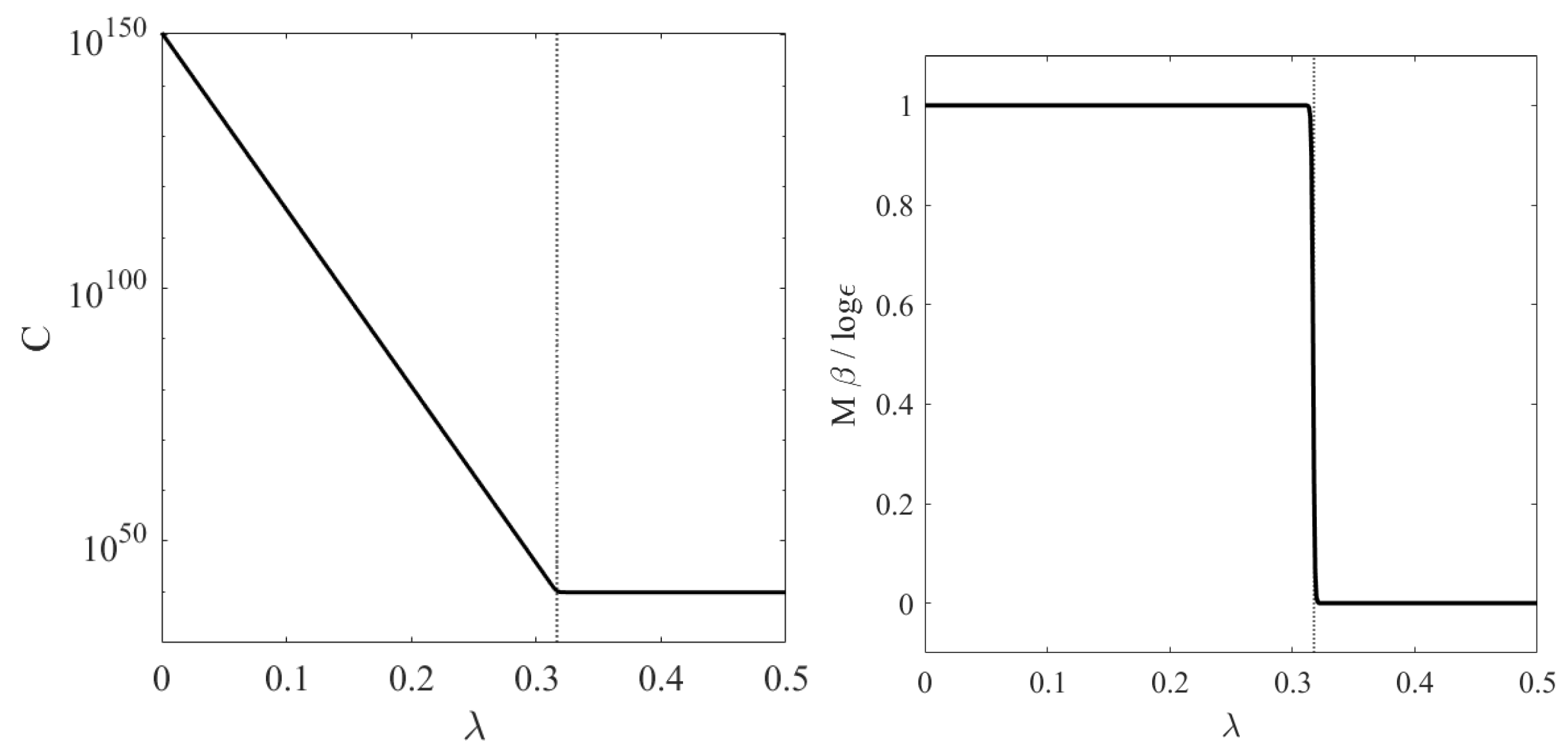
The behavior of $C_{\mathit{\lambda }}$ as a function of the normalized threshold $\mathit{\lambda }$ is illustrated in Figure 3.

Mimicking the theory of phase transitions, let us now look at the first derivative with respect to $\mathit{\lambda }$ of the quantity $\mathcal{F}=-{\mathit{\beta }}^{-1}logC$:

$$M:=-\frac{1}{N}\frac{\mathit{\partial }}{\mathit{\partial }\mathit{\lambda }}\mathcal{F}=-\frac{1}{N}\frac{\mathit{\partial }}{\mathit{\partial }\mathit{\lambda }}\left(-\frac{1}{\mathit{\beta }}logC(\mathit{\lambda })\right)$$

(22)

which, using Equation (19), and taking large N so that $T\approx \mathit{\lambda }N$, writes

$$M=\frac{log\mathit{ϵ}}{\mathit{\beta }}\frac{2^N{\mathit{ϵ}}^{\mathit{\lambda }N}}{{(1+\mathit{ϵ})}^N+2^N{\mathit{ϵ}}^{\mathit{\lambda }N}}=\frac{log\mathit{ϵ}}{2\mathit{\beta }}\left[1+tanh\left(\frac{N}{2}\left(\mathit{\lambda }-{\mathit{\lambda }}^{*}\right)log\mathit{ϵ}\right)\right]$$

(23)

The graph of $M(\mathit{\lambda })$, which acts as an order parameter for this model, is shown in the right panel of Figure 3 for $N=500$. At such moderate N, hence even more sharply in the large N limit, M undergoes a jump discontinuity at $\mathit{\lambda }={\mathit{\lambda }}^{*}$, which in statistical mechanics is typically associated with first-order phase transitions.

Suppose now that the threshold depends on time, so that $\mathit{\lambda }=\mathit{\lambda }\left(t\right)$, with $t=0,1$, constitutes a protocol in accord with the theory illustrated in Section 2.1, and ${\mathit{\mu }}_{\mathit{\lambda }\left(t\right)}$ is understood as the stationary distribution corresponding to a fixed value of t [31]. In particular, take the one-step transformation expressed by the protocol ${\mathit{\lambda }}_0\to {\mathit{\lambda }}_1$, with ${\mathit{\lambda }}_0\equiv \mathit{\lambda }\left(0\right)=0$ and ${\mathit{\lambda }}_1\equiv \mathit{\lambda }\left(1\right)\in [0,0.5]$. The associated stationary distributions can be computed using Equations (17) and (21). Specifically, denoting by ${\mathit{\mu }}_0\left(n\right)\equiv {\mathit{\mu }}_{{\mathit{\lambda }}_0}\left(n\right)$ the distribution evaluated at $\mathit{\lambda }={\mathit{\lambda }}_0$, we find

$${\mathit{\mu }}_0\left(n\right)=\frac{1}{2^N}\left(\genfrac{}{}{0pt}{}{N}{n}\right),$$

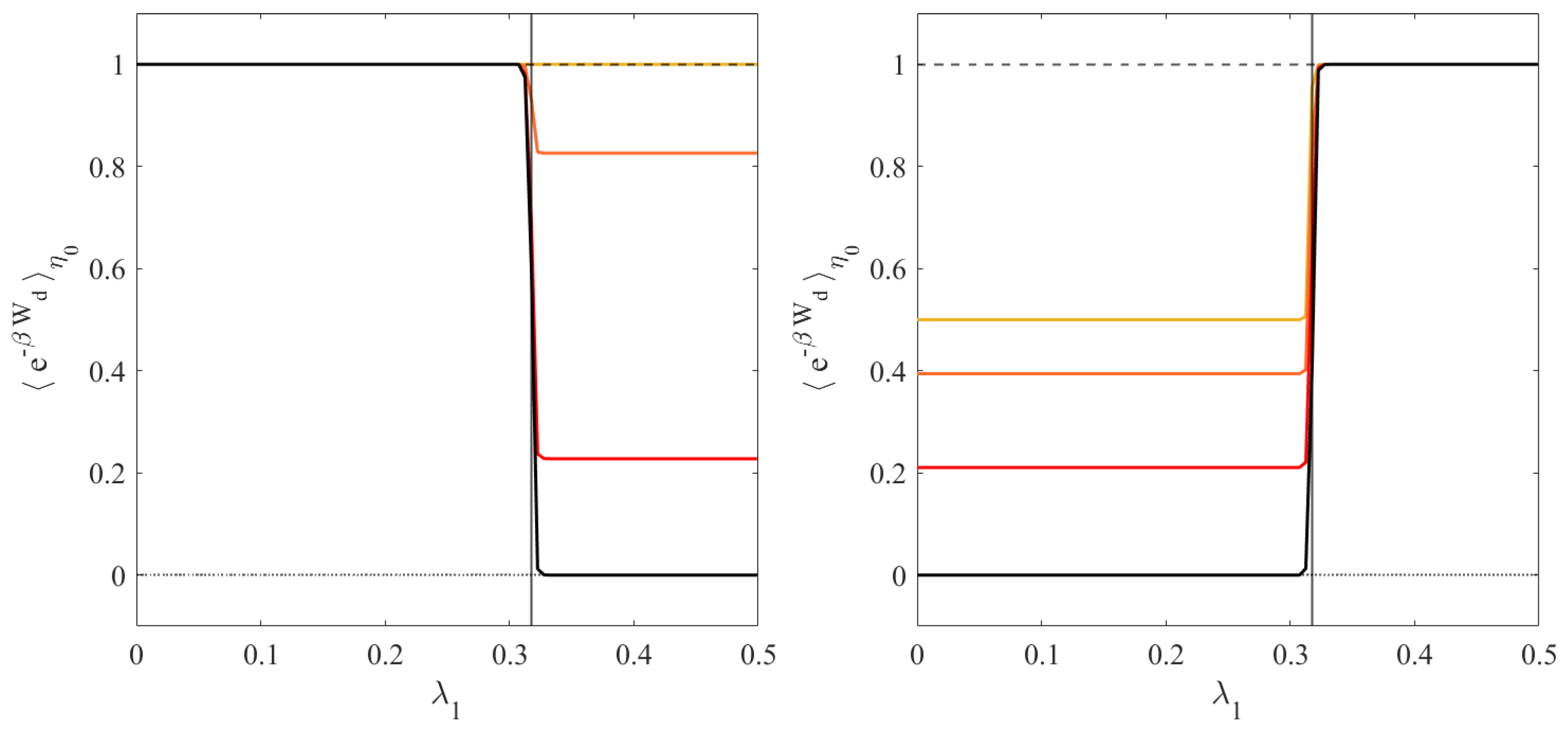
whereas ${\mathit{\mu }}_1\left(n\right)\equiv {\mathit{\mu }}_{{\mathit{\lambda }}_1}\left(n\right)$ depends on the final value ${\mathit{\lambda }}_1$ of the protocol. As discussed earlier in Section 2.2, a summation over all possible initial states $n\in {\mathcal{S}}_0=\{0,1,\dots ,N\}$ in Equation (10), which corresponds to no state space reduction ($\overline{\mathit{\mu }}=0$), yields the JE, regardless of the chosen value of ${\mathit{\lambda }}_1$. Specifically, for ${\mathit{\lambda }}^{*}<{\mathit{\lambda }}_1\le 0.5$, two symmetric steady states $n=n^{*}$ and $n=N-n^{*}$ appear. Indeed, we have ${\mathcal{S}}_0={\mathcal{S}}_1=\{0,1,\dots ,N\}$, and Equation (5) applies, independently of ${\mathit{\lambda }}_1$. Therefore, the JE does not reveal the jump discontinuity portrayed in the right panel of Figure 3, because it is not affected by that. The situation is different if the state space is reduced to a subset ${\mathit{\eta }}_0$ by a cutoff probability $\overline{\mathit{\mu }}>0$, see Equation (9). The left panel of Figure 4 shows indeed that ${〈e^{-\mathit{\beta }{W}_d}〉}_{{\mathit{\eta }}_0}\simeq 1$ for ${\mathit{\lambda }}_1<{\mathit{\lambda }}^{*}$, while a sudden drop to a value ${〈e^{-\mathit{\beta }{W}_d}〉}_{{\mathit{\eta }}_0}<1$ occurs for ${\mathit{\lambda }}_1>{\mathit{\lambda }}^{*}$. In fact, $\overline{\mathit{\mu }}$ as small as ${10}^{-20}$ suffices to get ${〈e^{-\mathit{\beta }{W}_d}〉}_{{\mathit{\eta }}_0}\simeq 0$ for ${\mathit{\lambda }}_1>{\mathit{\lambda }}^{*}$. This behavior signals the sudden separation of the state space regions occupied by the sets ${\mathit{\eta }}_0$ and ${\mathit{\eta }}_1$, in Equation (10), occurring at ${\mathit{\lambda }}_1={\mathit{\lambda }}^{*}$. While for ${\mathit{\lambda }}_1<{\mathit{\lambda }}^{*}$ the sets ${\mathit{\eta }}_0$ and ${\mathit{\eta }}_1$ overlap consistently, for ${\mathit{\lambda }}_1>{\mathit{\lambda }}^{*}$ one can safely consider $\mathcal{I}=\varnothing$, provided $\overline{\mathit{\mu }}$ is large enough. Thus, following the discussion of Section 2.2, for ${\mathit{\lambda }}_1>{\mathit{\lambda }}^{*}$ one expects not only that ${〈e^{-\mathit{\beta }{W}_d}〉}_{{\mathit{\eta }}_0}<1$, but also that, this average decreases for growing $\overline{\mathit{\mu }}$. This is indeed demonstrated in the left panel of Figure 4.

Consider now the one-step transformations with ${\mathit{\lambda }}_0=0.5$, which is larger than ${\mathit{\lambda }}^{*}$, and any ${\mathit{\lambda }}_1\in [0,1]$. In this case, the translational symmetry is broken because the initial condition selects only one of the two non-equilibrium states, say, the one with $n=n^{*}$. Then, taking $T=N/2$ in Equation (17) yields

$${\mathit{\mu }}_{\mathit{\lambda }=0.5}=\frac{1}{C_{0.5}}\left(\genfrac{}{}{0pt}{}{N}{n}\right){\mathit{ϵ}}^n,n<N/2.$$

where the second row of Equation (21) turns $C_{0.5}\approx {(1+\mathit{ϵ})}^N$, because only half of the state space $\mathcal{S}$ is involved. One obtains

$$\begin{array}{c}\hfill {\mathit{\mu }}_{\mathit{\lambda }\left(0\right)}\left(n\right)=\left\{\begin{array}{c}\frac{{\mathit{ϵ}}^n}{{(1+\mathit{ϵ})}^N}\left(\genfrac{}{}{0pt}{}{N}{n}\right)\mathrm{for}n<N/2\hfill \\ 0\mathrm{for}n\ge N/2\hfill \end{array}\right.\end{array}$$

which is supported on ${\mathcal{S}}_0=\{0,\dots ,N/2-1\}$, while the support of the distribution ${\mathit{\mu }}_{\mathit{\lambda }\left(1\right)}$ is ${\mathcal{S}}_1={\mathcal{S}}_0$ for ${\mathit{\lambda }}^{*}<{\mathit{\lambda }}_1\le 0.5$ (non-equilibrium phase) and ${\mathcal{S}}_1=\{0,\dots ,N\}$ for $0\le {\mathit{\lambda }}_1<{\mathit{\lambda }}^{*}$ (equilibrium phase). Consequently, Equation (5) holds for ${\mathit{\lambda }}^{*}<{\mathit{\lambda }}_1\le 0.5$ whereas Equation (13) applies for $0\le {\mathit{\lambda }}_1<{\mathit{\lambda }}^{*}$, because ${\mathcal{S}}_0\subset {\mathcal{S}}_1$, which implies:

$$\begin{array}{ccc}\hfill 〈e^{-\mathit{\beta }{W}_d\left(n\right)}〉& =& \sum _{n\in {\mathcal{S}}_0}{\mathit{\mu }}_1\left(n\right)=\sum _{n=0}^{T-1}\frac{{\mathit{ϵ}}^n}{2^N{\mathit{ϵ}}^T}\left(\genfrac{}{}{0pt}{}{N}{n}\right)+\sum _{n=T}^{N/2-1}\frac{1}{2^N}\left(\genfrac{}{}{0pt}{}{N}{n}\right)\hfill \\ & \simeq & \sum _{n=T}^{N/2-1}\frac{1}{2^N}\left(\genfrac{}{}{0pt}{}{N}{n}\right)\simeq 1/2,\hfill \end{array}$$

(24)

where the approximations turn exact for $T=0$ and $N\to \infty$. The violation of the JE stems from the “absolute irreversibility” of the process ${\mathit{\lambda }}_0\to {\mathit{\lambda }}_1$. This is illustrated by the numerical results reported in the right panel of Figure 4, which also clarifies the effect of reducing the state space with a cutoff probability $\overline{\mathit{\mu }}$. The effect is a $\overline{\mathit{\mu }}$ dependent further decrease of the average of $e^{-\mathit{\beta }{W}_d}$ for $0\le {\mathit{\lambda }}_1<{\mathit{\lambda }}^{*}$, visible in the left panel of Figure 4, cf. Equation (14).

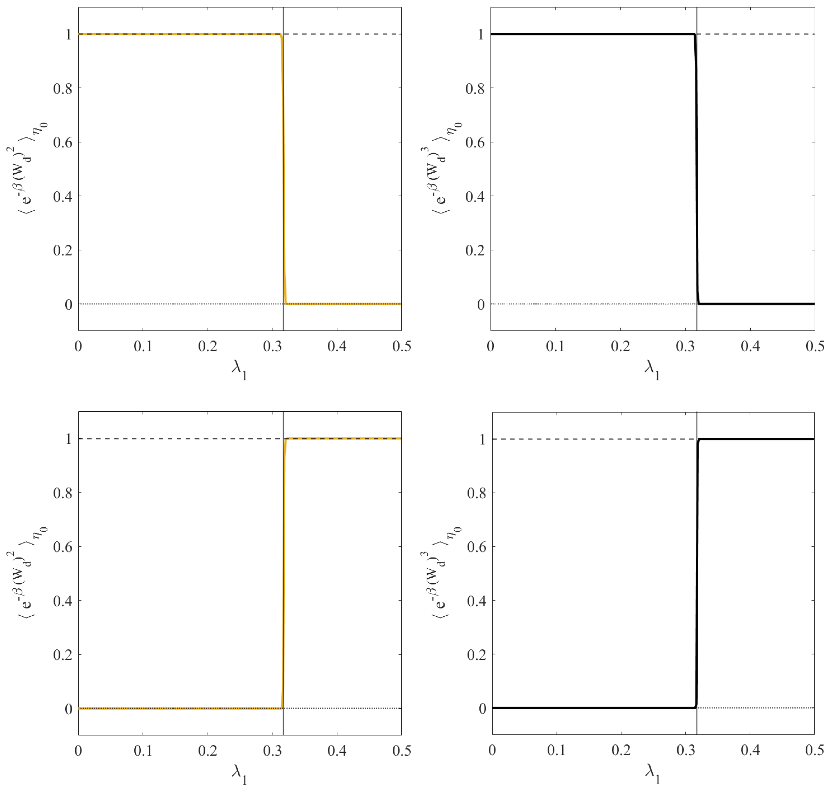
We conclude this Section observing that different exponential variables may be used to efficiently identify phase transitions. For instance, we considered $exp\{-\mathit{\beta }{\left(W_d\right)}^p\}$, with $p\in \mathbb{N}$, and numerically studied the cases $p=2$ and $p=3$. The numerical evaluation of ${\langle exp\{-\mathit{\beta }{\left(W_d\right)}^p\}\rangle }_{{\mathit{\eta }}_0}$ for the two different values of p and for different initial values of ${\mathit{\lambda }}_0$ is represented in Figure 5. It is important to note that, unlike the standard expression, corresponding to $p=1$, the quantity ${\langle e^{-\mathit{\beta }{\left(W_d\right)}^2}\rangle }_{{\mathit{\eta }}_0}$ displays a sharp transition at $\mathit{\lambda }={\mathit{\lambda }}^{*}$ even for $\overline{\mathit{\mu }}=0$, and not only for the truncated distributions. Moreover, ${\left(W_d\right)}^2$ is a quantity substantially different from $W_d$, because it only takes non-negative values, while negative values are fundamental for the usual fluctuation relations. This indicates that our approach may result effective with variables of quite different nature. Let us also note that taking higher odd powers of $W_d$, the calculation of the full state space averages may become prohibitive, from a computational point of view. Indeed, the negative values of $W_d$, raised to a large odd power and exponentiated, may result in being non-computable. However, our method based on truncated distributions may remain effective ( Figure 5 right panel) for $p=3$.

3.2. The 2D Ising Model

The second example we tackle is the classical 2D Ising model under an external magnetic field h, defined on a 2D lattice $\Lambda ={\{1,\dots ,L\}}^2$, with the state space $\mathcal{S}={\{-1,+1\}}^{\Lambda }$. Here, $\mathit{\beta }={\left(k_{B}T\right)}^{-1}$ denotes the inverse temperature. Let $\mathit{\sigma }\in \mathcal{S}$ denote a generic spin configuration, and introduce the Ising Hamiltonian, which reads

$$H(\mathit{\sigma })=-J\sum _{\begin{array}{c}\langle j,k\rangle \\ j,k\in \Lambda \end{array}}{\mathit{\sigma }}_j{\mathit{\sigma }}_k-h\sum _{j\in \Lambda }{\mathit{\sigma }}_j,$$

where ${\mathit{\sigma }}_j=\{-1,+1\}$ for $j\in \Lambda$, $J>0$ denotes the ferromagnetic coupling constant and the first sum is taken over pairs of adjacent spins (every pair is counted only once). Periodic boundary conditions are imposed along the horizontal and vertical directions. The model exhibits a critical value ${\mathit{\beta }}_c=ln(1+\sqrt{2})/2J$, marking the transition from a disordered (paramagnetic) to an ordered (ferromagnetic) phase. We then let the magnetic field depend on time and define a protocol $\mathit{\lambda }\left(t\right)=h\left(t\right)$. In [43], a similar problem is investigated, taking $\mathit{\lambda }\left(t\right)=J\left(t\right)$. We denote by $H_i(\mathit{\sigma })$ and $H_f(\mathit{\sigma })$ the Hamiltonians evaluated at the initial and the final values of the protocol, respectively, and we identify ${\mathit{\mu }}_k(\mathit{\sigma })=exp(-\mathit{\beta }{H}_k(\mathit{\sigma }))/Z_i$ as the Gibbs measure at the inverse temperature $\mathit{\beta }$, with $k=0,1$ and $Z_k={\sum }_{\mathit{\sigma }\in \mathcal{S}}exp(-\mathit{\beta }{H}_k(\mathit{\sigma }))$. So both ${\mathit{\mu }}_0$ and ${\mathit{\mu }}_1$ are supported on $\mathcal{S}$.

We now introduce the reduced state spaces ${\mathit{\eta }}_0=\{\mathit{\sigma }|{\mathit{\mu }}_0(\mathit{\sigma })\ge \overline{\mathit{\mu }}\}$ and ${\mathit{\eta }}_1=\{\mathit{\sigma }|{\mathit{\mu }}_1(\mathit{\sigma })\ge \overline{\mathit{\mu }}\}$ and we correspondingly denote ${\overline{Z}}_0={\sum }_{\mathit{\sigma }\in {\mathit{\eta }}_0}exp(-\mathit{\beta }{H}_0(\mathit{\sigma }))$ and ${\overline{Z}}_1={\sum }_{\mathit{\sigma }\in {\mathit{\eta }}_1}$$exp(-\mathit{\beta }{H}_1(\mathit{\sigma }))$. With the notation of Section 2.2, we have

$$1-{\mathit{\delta }}_k=\sum _{\mathit{\sigma }\in {\mathit{\eta }}_k}{\mathit{\mu }}_k(\mathit{\sigma })=\frac{{\sum }_{\mathit{\sigma }\in {\mathit{\eta }}_k}exp(-\mathit{\beta }{H}_k(\mathit{\sigma }))}{{\sum }_{\mathit{\sigma }\in \mathcal{S}}exp(-\mathit{\beta }{H}_k(\mathit{\sigma }))}=\frac{{\overline{Z}}_k}{Z_k},k=0,1,$$

(25)

which yields

$$\begin{array}{c}\hfill \frac{{\overline{Z}}_0}{{\overline{Z}}_1}=\frac{Z_0}{Z_1}\frac{1-{\mathit{\delta }}_0}{1-{\mathit{\delta }}_1}.\end{array}$$

Furthermore, for a function $f(\mathit{\sigma }):\mathcal{S}\to \mathbb{R}$, we set

$${\langle f\rangle }_{{\mathit{\eta }}_0}=\sum _{\mathit{\sigma }\in {\mathit{\eta }}_0}f(\mathit{\sigma })\frac{e^{-\mathit{\beta }{H}_0(\mathit{\sigma })}}{{\overline{Z}}_0}=\frac{1}{1-{\mathit{\delta }}_0}\sum _{\mathit{\sigma }\in {\mathit{\eta }}_0}f(\mathit{\sigma }){\mathit{\mu }}_0(\mathit{\sigma }).$$

(26)

Then, taking

$$f(\mathit{\sigma })=e^{-\mathit{\beta }{W}_d}=e^{-\mathit{\beta }(W-\Delta F)}=e^{-\mathit{\beta }(H_1(\mathit{\sigma })-H_0(\mathit{\sigma }))}\frac{Z_0}{Z_1},\mathrm{where}\mathit{\beta }\Delta F=log\frac{Z_0}{Z_1},$$

we find

$$f(\mathit{\sigma }){\mathit{\mu }}_0(\mathit{\sigma })=\frac{e^{-\mathit{\beta }{H}_1(\mathit{\sigma })}}{Z_0}\frac{Z_0}{Z_1}={\mathit{\mu }}_1(\mathit{\sigma }),$$

and

$$\begin{array}{ccc}\hfill {〈e^{-\mathit{\beta }{W}_d}〉}_{{\mathit{\eta }}_0}& =& \frac{1}{1-{\mathit{\delta }}_0}\sum _{\mathit{\sigma }\in {\mathit{\eta }}_0}{\mathit{\mu }}_1(\mathit{\sigma }).\hfill \end{array}$$

(27)

The latter equation coincides with Equation (10) and recovers Equation (14) [43]. We are interested in studying the application of Equation (27) to evolutions in which the magnetic field changes from ${\mathit{\lambda }}_0=h_0$ to ${\mathit{\lambda }}_1=h_1$. Setting $J=1$, which yields ${\mathit{\beta }}_c\approx 0.4406$, we consider different scenarios. We first choose $\mathit{\beta }>{\mathit{\beta }}_c$, so that the 2D Ising model undergoes a first-order phase transition when the magnetic field h changes sign, and we study the behavior of ${\langle e^{-\mathit{\beta }{W}_d}\rangle }_{{\mathit{\eta }}_0}$ as a function of $h_1$. Later, we study the case with $\mathit{\beta }<{\mathit{\beta }}_c$, where no phase transition takes place. The computation of ${\langle e^{-\mathit{\beta }{W}_d}\rangle }_{{\mathit{\eta }}_0}$ can be conveniently carried out by sampling configurations $\mathit{\sigma }\in \mathcal{S}$, with a prescribed magnetization density $m=N^{-1}{\sum }_{j\in \Lambda }{\mathit{\sigma }}_j$, from the distribution [43]:

$$P\left(m\right)=\sum _{\mathit{\sigma }\in \mathcal{S}}\mathit{\mu }(\mathit{\sigma })\mathit{\delta }\left(m-\frac{1}{N}\sum _{j\in \Lambda }{\mathit{\sigma }}_{j\in \Lambda }\right)$$

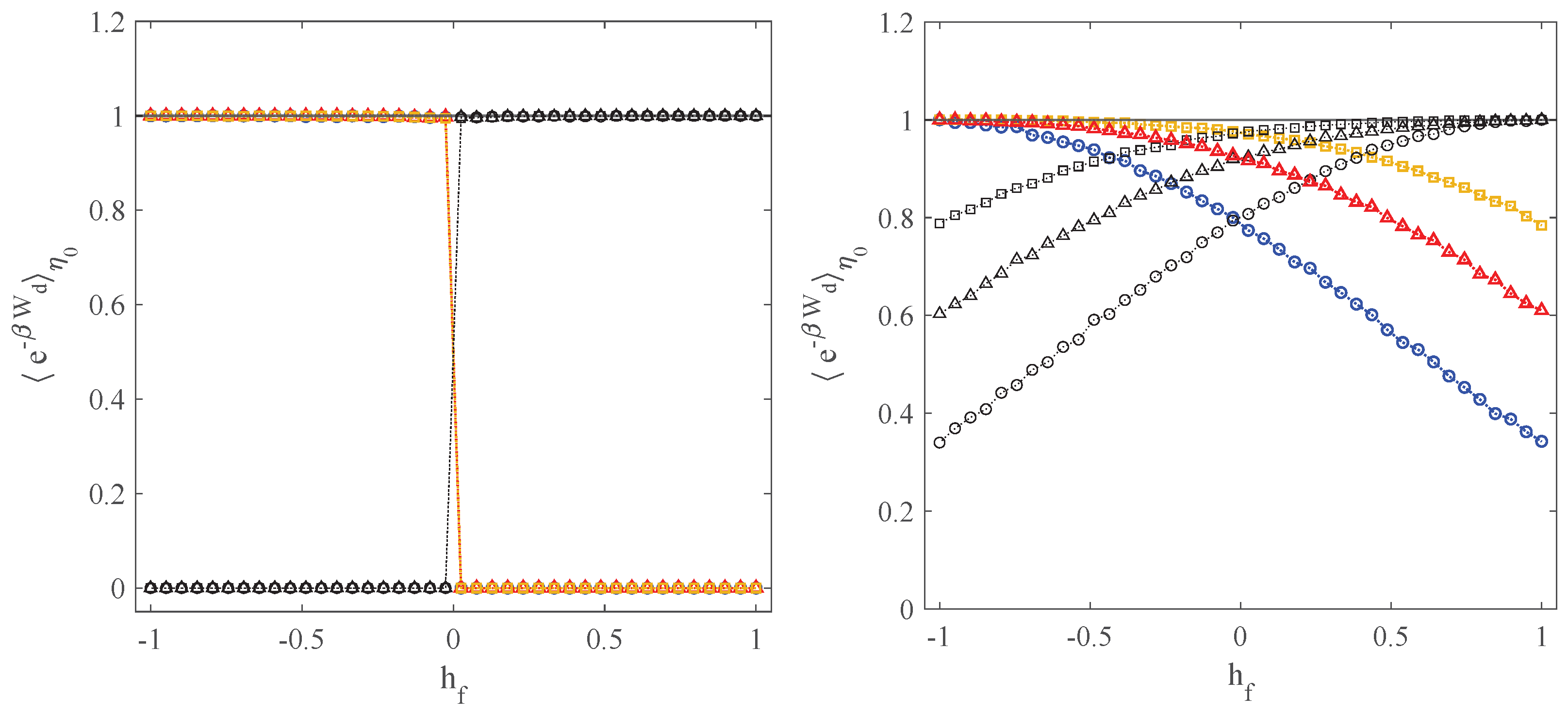
Figure 6 shows that $\langle e^{-\mathit{\beta }{W}_d}\rangle =1$ when $\overline{\mathit{\mu }}=0$, for both $\mathit{\beta }<{\mathit{\beta }}_c$ and $\mathit{\beta }>{\mathit{\beta }}_c$, cf. Equation (5). Therefore, the phase transition in the Ising model is not detected by the JE in one-step transformations. For the reduced state spaces, corresponding to cutoffs $\overline{\mathit{\mu }}>0$, the situation changes, as evidenced by the left panel of Figure 6. The phase transition is properly captured by ${\langle e^{-\mathit{\beta }{W}_d}\rangle }_{{\mathit{\eta }}_0}$, which drops abruptly from the value 1 to a value close to 0 when crossing $h_1=0$, for $h_0=-1$ and with $h_1\in [-1,1]$. An analogous behavior is also observed when $h_0=1$ and $h_1$ is varied in the same interval. It is worth recalling that, in the Curie–Weiss approximation of the Ising model, the value of the magnetization density m is obtained from the solution of the mean field equation $m=tanh[\mathit{\beta }(m+h\left)\right]$, which, for $\mathit{\beta }>{\mathit{\beta }}_c$, gives rise to metastable branches [60]. One such branch corresponds to positive values of m in the interval $[-h_c,0]$, and another branch corresponds, symmetrically, to negative values of m in the interval $[0,h_c]$, with $h_c>0$. This is not visible in the left panel of Figure 6, which shows that for $h_0=\pm 1$ the discontinuity occurs in both cases sharply at $h_1=0$. This is a consequence of our choice of initial datum for the Monte Carlo simulations, that mitigates the effects of the two metastable branches. More precisely, as initial datum we took ${\mathit{\sigma }}_j=-1$ for $h_1<0$ and ${\mathit{\sigma }}_j=1$ for $h_1>0$, for all $j\in \Lambda$, producing a distribution $P\left(m\right)$ sharply concentrated near $m=-1$ for $h_1<0$ and near $m=1$ for $h_1>0$. The discontinuity at $h_1=0$, therefore, stems from Equation (12), which rules the behavior of ${\langle e^{-\mathit{\beta }{W}_d}\rangle }_{{\mathit{\eta }}_0}$ for $\mathit{\beta }>{\mathit{\beta }}_c$, where one can assume $\mathcal{I}=\varnothing$. In the left panel, it is also interesting to note that, for $\mathit{\beta }=2.5>{\mathit{\beta }}_c$, the different sets of data points corresponding to different values of $\overline{\mathit{\mu }}$ fully overlap with one another and display the same discontinuity at $h_1=0$.

For $\mathit{\beta }<{\mathit{\beta }}_c$ the phase transition in the Ising model is instead absent, and the magnetization density m solving the mean field equation becomes a continuous function of h, which vanishes at $h=0$. As a result, the data points shown in the right panel of Figure 6 show that ${\langle e^{-\mathit{\beta }{W}_d}\rangle }_{{\mathit{\eta }}_0}$ no longer presents a sharp discontinuity at $h_1=0$, as this quantity decreases in a continuous fashion while increasing the difference $|h_0-h_1|$. The effect of varying the value of $\overline{\mathit{\mu }}$ is clearly visible in the right panel. Again, the JE is not affected by the variation of $h_1$.

4. Conclusions

In this study, we propose one way of benefiting from incomplete statistics or finite-size effects, which result in a reduction in the state space. As this is often an unavoidable fact, we show that it can provide valuable insight, if associated with exponential observables. In particular, we have considered the Jarzynski Equality and its instantaneous transformation variant (also known as Free Energy Perturbation), to identify the critical values of the parameters corresponding to a first-order phase transition. Smooth variations of states have also been characterized. This is due to the sensitivity of exponentials of extensive quantities, when averaged over the available subsets of the system state space, which is usually considered a hindrance. Interestingly enough, our study shows that reducing the amount of available information about the system can enhance our understanding of its critical behaviors. In fact, this is not obtained from a perfect sampling of states. The JE, in particular, results are insensitive to parameters variations, hiding interesting features of the system at hand.

We illustrated our theoretical findings by numerically analyzing two stochastic models: a modified Ehrenfest urn model and a classical 2D Ising model subject to an external magnetic field. In both cases, we observed a jump discontinuity in the quantity ${\langle e^{-\mathit{\beta }{W}_d}\rangle }_{{\mathit{\eta }}_0}$ occurring at the same value of the control parameter distinguishing different macroscopic phases in the thermodynamic limit of the model, remaining quite far from that limit. Similarly, when the phase transition is absent, as in the case of the Ising model at supercritical temperatures, the variation of state with the control parameter, is still revealed by a continuous variation of ${\langle e^{-\mathit{\beta }{W}_d}\rangle }_{{\mathit{\eta }}_0}$.

Studying the behavior of powers of $W_d$ we also found that our approach works even with variables different from those of fluctuation theorems. Indeed, it provides a new recipe to identify order parameters in the study of non-equilibrium phase transitions, which is particularly effective with truncated distributions.

Future works are intended to develop this approach, so that incomplete information on a given system may be used beyond the problem of discovering phase transitions.

References

1. Bennett, C.H. Efficient estimation of free energy differences from monte carlo data. J. Comput. Phys. 1976, 22, 245–268. [Google Scholar] [CrossRef]
2. Widom, B. Some topics in the theory of fluids. J. Chem. Phys. 1963, 39, 2808–2812. [Google Scholar] [CrossRef]
3. Zwanzig, R.W. High-temperature equation of state by a perturbation method. ii. Polar gases. J. Chem. Phys. 1955, 23, 1915–1922. [Google Scholar] [CrossRef]
4. Evans, D.J.; Searles, D.J. The fluctuation theorem. Adv. Phys. 2002, 52, 1529. [Google Scholar] [CrossRef]
5. Evans, D.J.; Cohen, E.G.D.; Morriss, G.P. Probability of second law violations in shearing steady states. Phys. Rev. Lett. 1993, 71, 2401. [Google Scholar] [CrossRef] [PubMed]
6. Jepps, O.G.; Rondoni, L. A dynamical-systems interpretation of the dissipation function, T-mixing and their relation to thermodynamic relaxation. J. Phys. A Math. Theor. 2016, 49, 154002. [Google Scholar] [CrossRef]
7. Jarzynski, C. Non-equilibrium equality for free energy differences. Phys. Rev. Lett. 1997, 78, 2690. [Google Scholar] [CrossRef]
8. Crooks, G.E. Non-equilibrium measurements of free energy differences for microscopically reversible markovian systems. J. Stat. Phys. 1998, 90, 1481–1487. [Google Scholar] [CrossRef]
9. Crooks, G.E. Path-ensemble averages in systems driven far from equilibrium. Phys. Rev. E 2000, 61, 2361–2366. [Google Scholar] [CrossRef]
10. Hatano, T.; Sasa, S. Steady-state thermodynamics of langevin systems. Phys. Rev. Lett. 2001, 86, 3463. [Google Scholar] [CrossRef]
11. Marconi, U.M.B.; Puglisi, A.; Rondoni, L.; Vulpiani, A. Fluctuation–dissipation: Response theory in statistical physics. Phys. Rep. 2008, 461, 111–195. [Google Scholar] [CrossRef]
12. Seifert, U. Stochastic thermodynamics, fluctuation theorems and molecular machines. Rep. Prog. Phys. 2012, 75, 126001. [Google Scholar] [CrossRef]
13. Cohen, E.G.D.; Mauzerall, D. A note on the jarzynski equality. J. Stat. Mech. Theory Exp. 2004, 2004, P07006. [Google Scholar] [CrossRef]
14. Vilar, J.M.G.; Rubi, J.M. Failure of the work-hamiltonian connection for free-energy calculations. Phys. Rev. Lett. 2008, 100, 020601. [Google Scholar] [CrossRef] [PubMed]
15. Talkner, P.; Hänggi, P. Open system trajectories specify fluctuating work but not heat. Phys. Rev. E 2016, 94, 022143. [Google Scholar] [CrossRef] [PubMed]
16. Peliti, L. On the work—Hamiltonian connection in manipulated systems. J. Stat. Mech. Theory Exp. 2008, 2008, P05002. [Google Scholar] [CrossRef]
17. Vilar, J.M.G.; Rubi, J.M. Vilar and rubi reply. Phys. Rev. Lett. 2008, 101, 098902. [Google Scholar] [CrossRef]
18. Ciliberto, S. Experiments in stochastic thermodynamics: Short history and perspectives. Phys. Rev. X 2017, 7, 021051. [Google Scholar] [CrossRef]
19. Liphardt, J.; Dumont, S.; Smith, S.B.; Tinoco, I.; Bustamante, C. Equilibrium information from non-equilibrium measurements in an experimental test of jarzynski’s equality. Science 2002, 296, 1832–1835. [Google Scholar] [CrossRef]
20. Monge, A.M.; Manosas, M.; Ritort, F. Experimental test of ensemble inequivalence and the fluctuation theorem in the force ensemble in dna pulling experiments. Phys. Rev. E 2018, 98, 032146. [Google Scholar] [CrossRef]
21. Peliti, L. Comment on “failure of the work-hamiltonian connection for free-energy calculations”. Phys. Rev. Lett. 2008, 101, 098903. [Google Scholar] [CrossRef] [PubMed]
22. Bustamante, C.; Liphardt, J.; Ritort, F. The Non-equilibrium Thermodynamics of Small Systems. Phys. Today 2005, 58, 43–48. [Google Scholar] [CrossRef]
23. Lua, R.C.; Grosberg, A.Y. Practical applicability of the jarzynski relation in statistical mechanics: A pedagogical example. J. Phys. Chem. B 2005, 109, 6805–6811. [Google Scholar] [CrossRef] [PubMed]
24. Crooks, G.E.; Jarzynski, C. Work distribution for the adiabatic compression of a dilute and interacting classical gas. Phys. Rev. E 2007, 75, 021116. [Google Scholar] [CrossRef] [PubMed]
25. Jarzynski, C. Stochastic and macroscopic thermodynamics of strongly coupled systems. Phys. Rev. X 2017, 7, 011008. [Google Scholar] [CrossRef]
26. Hansen, N.; Van Gunsteren, W.F. Practical aspects of free-energy calculations: A review. J. Chem. Theory Comput. 2014, 10, 2632–2647. [Google Scholar] [CrossRef]
27. Torrie, G.M.; Valleau, J.P. Nonphysical sampling distributions in monte carlo free-energy estimation: Umbrella sampling. J. Comput. Phys. 1977, 23, 187–199. [Google Scholar] [CrossRef]
28. Pohorille, A.; Jarzynski, C.; Chipot, C. Good practices in free-energy calculations. J. Phys. Chem. B 2010, 114, 10235–10253. [Google Scholar] [CrossRef]
29. Wu, D.; Kofke, D.A. Phase-space overlap measures. ii. Design and implementation of staging methods for free-energy calculations. J. Chem. Phys. 2005, 123, 084109. [Google Scholar] [CrossRef]
30. Colangeli, M.; Di Francesco, A.; Rondoni, L. Finite Reservoirs Corrections to Hamiltonian Systems Statistics and Time Symmetry Breaking. Symmetry 2023, 15, 1268. [Google Scholar] [CrossRef]
31. Hack, P.; Gottwald, S.; Braun, D.A. Jarzyski’s Equality and Crooks’ Fluctuation Theorem for General Markov Chains with Application to Decision-Making Systems. Entropy 2022, 42, 1731. [Google Scholar] [CrossRef]
32. Ge, H.; Qian, M. Generalized Jarzynski’s equality in inhomogeneous Markov chains. J. Math. Phys. 2007, 48, 053302. [Google Scholar] [CrossRef]
33. Horowitz, J.M.; Vaikuntanathan, S. Non-equilibrium detailed fluctuation theorem for repeated discrete feedback. Phys. Rev. E 2010, 82, 061120. [Google Scholar] [CrossRef] [PubMed]
34. Murashita, Y.; Funo, K.; Ueda, M. Non-equilibrium equalities in absolutely irreversible processes. Phys. Rev. E 2014, 90, 042110. [Google Scholar] [CrossRef] [PubMed]
35. Murashita, Y.; Ueda, M. Gibbs paradox revisited from the fluctuation theorem with absolute irreversibility. Phys. Rev. Lett. 2017, 118, 060601. [Google Scholar] [CrossRef] [PubMed]
36. Funo, K.; Murashita, Y.; Ueda, M. Quantum non-equilibrium equalities with absolute irreversibility. New J. Phys. 2015, 17, 075005. [Google Scholar] [CrossRef]
37. Manikandan, S.K.; Elouard, C.; Jordan, A.N. Fluctuation theorems for continuous quantum measurements and absolute irreversibility. Phys. Rev. A 2019, 99, 022117. [Google Scholar] [CrossRef]
38. Cirillo, E.N.; Colangeli, M.; Muntean, A.; Richardson, O.; Rondoni, L. Deterministic reversible model of non-equilibrium phase transitions and stochastic counterpart. J. Phys. A Math. Theor. 2020, 53, 305001. [Google Scholar] [CrossRef]
39. Stroock, D.J. An Introduction to Markov Processes; Springer: Berlin/Heidelberg, Germany, 2005. [Google Scholar]
40. Billingsley, P. Probability and Measures; John Wiley & Sons: Hoboken, NJ, USA, 1995. [Google Scholar]
41. Feller, W. An Introduction to Probability. Theory and Applications; John Wiley & Sons: Hoboken, NJ, USA, 1968. [Google Scholar]
42. Sekimoto, K. Stochastic Energetics; Springer: Berlin/Heidelberg, Germany, 2010. [Google Scholar]
43. Hoang, D.-T.; Venkatesh, B.P.; Han, S.; Jo, J.; Watanabe, G.; Choi, M.-S. Scaling law for irreversible entropy production in critical systems. Sci. Rep. 2016, 6, 27603. [Google Scholar] [CrossRef]
44. Kac, M. Probability and Related Topics in Physical Sciences, 1 of Lectures in Applied Mathematics; Interscience Publishers: Geneva, Switzerland, 1959. [Google Scholar]
45. Cirillo, E.N.; Colangeli, M.; Richardson, O.; Rondoni, L. Deterministic model of battery, uphill currents, and nonequilibrium phase transitions. Phys. Rev. E 2021, 103, 032119. [Google Scholar] [CrossRef]
46. Cirillo, E.N.; Colangeli, M.; Di Francesco, A.; Kröger, M.; Rondoni, L. Transport and nonequilibrium phase transitions in polygonal urn models. Chaos Interdiscip. J. Nonlinear Sci. 2022, 32, 093127. [Google Scholar] [CrossRef] [PubMed]
47. Cirillo, E.N.; Colangeli, M.; Kröger, M.; Rondoni, L. Nonequilibrium phase transitions in feedback-controlled three-dimensional particle dynamics. Phys. Rev. Res. 2023, 5, 043063. [Google Scholar] [CrossRef]
48. Godreche, C.; Luck, J.M. Non-equilibrium dynamics of urn models. J. Phys. Condens. Mat. 2002, 14, 1601–1615. [Google Scholar] [CrossRef]
49. Dette, H. On a generalization of the Ehrenfest urn model. J. Appl. Prob. 1994, 31, 930–939. [Google Scholar] [CrossRef]
50. Ohkubo, J.; Yasuda, M.; Tanaka, K. Preferential urn model and nongrowing complex networks. Phys. Rev. E 2005, 72, 065104. [Google Scholar] [CrossRef] [PubMed]
51. Siegmund, D.; Yakir, B. An urn model of diaconis. Annal. Prob. 2005, 33, 2036–2042. [Google Scholar] [CrossRef]
52. Chen, M.-R.; Hsiau, S.-R. On a generalized q-urn model. Prob. Eng. Sci. 2015, 29, 99–115. [Google Scholar] [CrossRef]
53. Idriss, S. Nonlinear unbalanced urn models via stochastic approximation. Meth. Comput. Appl. Prob. 2022, 24, 413–430. [Google Scholar] [CrossRef]
54. Zhang, L.-X.; Hu, F.; Cheung, S.H.; Chan, W.S. Asymptotic properties of multicolor randomly reinforced Pólya urns. Adv. Appl. Prob. 2014, 46, 585–602. [Google Scholar] [CrossRef]
55. Kao, Y.M.; Luan, P.G. Poincare cycle of a multibox Ehrenfest urn model with directed transport. Phys. Rev. E 2003, 67, 031101. [Google Scholar] [CrossRef]
56. Chen, M.-R.; Kuba, M. On generalized Pólya urn models. J. Appl. Prob. 2013, 50, 1169–1186. [Google Scholar] [CrossRef]
57. Bai, Z.D.; Hu, F.F.; Zhang, L.X. Gaussian approximation theorems for urn models and their applications. Annal. Appl. Prob. 2002, 12, 1149–1173. [Google Scholar] [CrossRef]
58. Klein, M.J. Entropy and the Ehrenfest urn model. Physica 1956, 22, 569–575. [Google Scholar] [CrossRef]
59. Thornblad, E. The dominating colour of an infinite Pólya urn model. J. Appl. Prob. 2016, 53, 914–924. [Google Scholar] [CrossRef]
60. Presutti, E. Scaling Limits in Statistical Mechanics and Microstructures in Continuum Mechanics; Springer: Berlin/Heidelberg, Germany, 2009. [Google Scholar]
Figure 1. Top row: Gaussian distributions centered at x ¯ 0 = 4 (left panel): μ 0 ( x ) has standard deviation σ 0 = 0.5 (black), while the standard deviation of μ 1 ( x ) is σ 1 = 0.3 (red) and 0.7 (blue). The horizontal dashed line denotes the value μ ¯ , which determines η 0 = [ x ¯ 0 Δ , x ¯ 0 + Δ ] . (right panel): behavior of e β W d η 0 as a function of σ 1 / σ 0 for different values of Δ , computed using Equation (12). Bottom row, (left panel): μ 0 ( x ) is a Gaussian centered at x ¯ 0 = 3 with standard deviation σ 0 = 0.5 (black curve), while μ 1 ( x ) is a Gaussian function centered at x ¯ 1 = 5 with standard deviations σ 1 = 0.3 (blue), 0.5 (green), 0.7 (red). (right panel): graph of e β W d η 0 as a function of Δ / ( x ¯ 0 x ¯ 1 ) for different values of σ 1 , computed using Equation (12).
Symmetry 16 00125 g001
Figure 2. Stationary distributions for N = 500 . Right panel: stability regions in the ϵ - λ parameter space. White corresponds to stable equilibrium ( n = N / 2 ); cyan to two metastable non-equilibrium states ( n = n * , N n * ) and stable equilibrium; and brown to two stable non-equilibrium states and metastable equilibrium. The remaining three panels, from left to right, plot with vertical log-scale the stationary distributions (17) referring to the points A = ( 0.2 , 0.1 ) , B = ( 0.2 , 0.25 ) and C = ( 0.2 , 0.4 ) .
Symmetry 16 00125 g002
Figure 3. Left panel: Normalization constant C λ as a function of λ , Equation (19), with vertical axis in logarithmic scale. Dotted vertical line indicates the critical value λ * defined in Equation (20). Right panel: M ( λ ) β / log ϵ obtained through Equation (23), with dotted vertical line indicating the critical value λ * . Both plots are obtained for N = 500 , β = 1 and ϵ = 0.2 .
Symmetry 16 00125 g003
Figure 4. Numerical estimation of e β W d η 0 , as a function of λ 1 , given by Equation (10). The yellow, orange, red, and black lines correspond to cutoffs μ ¯ = 0 , 10 60 , 10 50 , 10 20 , respectively. The vertical solid black lines lie at λ = λ * . The dashed black lines correspond to Equation (5). N, β and ϵ are set to the same values considered in Figure 3. Left panel: The process starts in a homogeneous state with λ 0 = 0 . The yellow line is always at 1; the phase transition is only revealed by the truncated distributions. Right panel: The process starts in a non-homogeneous state with λ 0 = 0.5 . The values for μ ¯ = 0 and λ < λ * do not equal 1, as prescribed by Equation (24). Even the full distribution reveals the phase transition.
Symmetry 16 00125 g004
Figure 5. Numerical estimation of e β ( W d ) p η 0 as a function of λ 1 for p = 2 and p = 3 (left and right column, respectively), with the parameters N, β , and ϵ set to the same values as in Figure 3. The plots refer to a process starting in a homogeneous state with λ 0 = 0 (top row) or in a non-homogeneous state with λ 0 = 0.5 (bottom row). In the left panels, the yellow line refers to the cutoff μ ¯ = 0 , whereas the curves corresponding to cutoff values μ ¯ > 0 are not shown in the plots, as they are graphically indistinguishable from the yellow line. In the right panels, the solid black line refers to the cutoff μ ¯ = 10 15 .
Symmetry 16 00125 g005
Figure 6. e β W d η 0 as a function of h f , Equation (27), from Monte Carlo simulations of a 2D Ising model on a square grid of linear size L = 10 . Here, J = 1 , hence β c 0.4406 , and periodic boundary conditions are applied in both horizontal and vertical directions. Simulations have been performed with h i = 1 (colored symbols) and h i = 1 (black symbols), for β = 2.5 > β c (left panel) and β = 0.1 < β c (right panel). Circles, triangles, and squares correspond to μ ¯ = ( max { μ 0 } + max { μ 1 } ) / ( 2 k ) with k = 5 , 25 , 100 , respectively. The horizontal black line at 1 represents in both panels the case with μ ¯ = 0 .
Symmetry 16 00125 g006
Disclaimer/Publisher’s Note: The statements, opinions and data contained in all publications are solely those of the individual author(s) and contributor(s) and not of MDPI and/or the editor(s). MDPI and/or the editor(s) disclaim responsibility for any injury to people or property resulting from any ideas, methods, instructions or products referred to in the content.