Abstract
Traditional numerical methods often provide local solutions for initial value problems of differential equations, even though these problems may have solutions over larger intervals. Current neural network algorithms and deep learning methods also struggle to ensure solutions across these broader intervals. This paper introduces a novel approach employing piecewise neural networks to address this issue. The method involves dividing the solution interval into smaller segments and utilizing neural networks with a uniform structure to solve sub-problems within each segment. These solutions are then combined to form a piecewise expression representing the overall solution. The approach guarantees continuous differentiability of the obtained solution over the entire interval, except for finite end points of those sub-intervals.To enhance accuracy, parameter transfer and multiple rounds of pre-training are employed. Importantly, this method maintains a consistent network size and training data scale across sub-domains, unlike existing neural network algorithms. Numerical experiments validate the efficiency of the proposed algorithm.
1. Introduction
As we know, constrained by convergence requirements, various traditional numerical solution methods, such as Picard approximation and Runge–Kutta methods, for initial value problems (IVPs) of differential equations or dynamic systems (ODEs) are typically suitable only for local solutions within a neighborhood interval of the initial value point, even if the problem possesses larger interval (global) solutions. Consequently, extending a local solution to a larger interval remains a fundamental challenge in the field of numerical solutions to ODE problems, which has yet to be fully addressed [1,2].
Currently, the artificial neural network (ANN) algorithm, as a novel numerical solution method for solving differential equation problems, is rapidly evolving and attracting attention and exploration from many researchers [3]. Although the ANN algorithm, like traditional methods, performs well mainly in the neighborhood of the initial value point and lacks inherent learning capability on large intervals, it offers numerous advantages in solving IVPs of ODEs. For instance, the neural network-based solution to a differential equation is differentiable and presented in closed analytic form, suitable for subsequent calculations. It is independent of discrete schemes and the shape of the variable domain. Therefore, it is anticipated that the aforementioned solution extension problem can be effectively addressed through the enhancement and efficient utilization of the ANN algorithm. In this paper, we propose a piecewise neural network (PWNN) method to tackle this problem.
Before describing our algorithm, let us briefly review the development profile of ANN algorithms for solving differential equation problems.
The theoretical foundation supporting the use of ANN algorithms for solving differential equation problems lies in the general approximation theorems provided by Hornik, Womik, and Li X et al. [4,5,6], which theoretically establish that any continuous function can be approximated by a neural network. Subsequently, a widely utilized ANN algorithm for solving differential equations with initial boundary value conditions was introduced by Lagaris et al. [7]. However, for problems involving more complex initial boundary values, this method faces difficulties in constructing the necessary trial solutions for the underlying problems.
Another significant development in ANN algorithms for solving differential equation problems is the implementation of automatic differentiation technology [8,9,10,11], which has led to the proliferation of ANN methods for solving differential equation problems and their broader application. Building upon this technique, Justin Sirignano and Konstantinos Spiliopoulos proposed the Deep Galerkin Method (DGM), a deep neural network method for solving (partial) differential equation problems in higher dimensions [12]. Anitescu et al. introduced an ANN method utilizing adaptive configuration strategies to enhance method robustness and reduce computational costs in solving boundary value problems of differential equations [13].
A landmark advancement in ANN algorithms for solving differential equation problems was the introduction of physical information neural networks (PINN) by Raissi et al. [14]. In this method, the initial boundary conditions of the differential equation are incorporated into the loss function, allowing the ANN to directly express an approximate solution to the differential equation. This eliminates the need to construct a trial solution according to equations and initial boundary value conditions, as required by Lagaris’s method. Subsequently, numerous ANN algorithms based on PINN have been developed rapidly. For example, Lei Yuan and Ni et al. introduced the Auxiliary PINN (A-PINN), capable of bypassing limitations in integral discretization and solving forward and inverse problems of nonlinear integral differential equations [15]. Chiu et al. proposed novel PINN methods for coupling neighboring support points and their derivative terms obtained by automatic differentiation [16]. Huang et al. combined PINN with the homotopy continuation method, proposing Homotopy PINN (HomPINN) for solving multiple solutions of nonlinear elliptic differential equations, overcoming the limitation of PINN in finding only the flattest solution in most cases [17]. Yin et al. utilized PINN to address a range of femtosecond optical soliton solutions pertaining to the high-order nonlinear Schrdinger equation [18]. Based on the PINN method, Yuexing et al. proposed an enhanced version of PINN called IPINN, introducing localized adaptive activation functions to improve performance, successfully applying the method to solve several differential equation models in finance [19]. Meng et al. introduced a modified PINN method called PPINN, dividing a long-period problem into a series of short-period ones to accelerate the training of ANN algorithms [20].
Moreover, there are numerous other analogs of PINN-based studies and various types of ANN methods. For instance, convolutional ANN methods [21,22,23] and theoretically guided ANN methods [24,25] have also been employed to explore new solution methods for (partial) differential equations. Particularly noteworthy is the work of Run-Fa Zhang and Sudao Bilige, who proposed bilinear neural networks, the first attempt to obtain analytical solutions to nonlinear partial differential equations using the ANN method [26,27].
Importantly, a general observation from this literature is that ANN algorithms for solving IVPs of differential equations perform well in relatively small domains near the initial value point but sometimes exhibit poor convergence over large intervals. To obtain a large interval solution, it is often necessary to enhance the training data and expand the network size (depth and width). However, doing so not only reduces computational efficiency but also makes it challenging to guarantee obtaining a large interval solution to the problem. Therefore, alternative strategies are being explored to enhance the efficiency of ANN algorithms. For example, various adaptive activation functions [19,28,29,30] and adaptive weights [31,32] have been proposed. The key feature of these studies is the introduction of hyperparameters into traditional activation functions to adjust ANN convergence. Studies by Jaftap et al. have shown that these methods are primarily effective in the early stages of network training [33]. Adaptive weights leverage gradient statistics to optimize the interplay between various components in the loss function by incorporating additional weighting during the training process. While these solutions alleviate the convergence difficulties of neural networks in complex problems from different perspectives, there is insufficient evidence to demonstrate that simultaneously using different optimization schemes can still reduce network training difficulty and achieve large interval solutions. To solve the IVP of dynamic systems, Wen et al. proposed an ANN algorithm based on the Lie symmetry of differential equations [34,35,36,37]. This novel approach combines Lie group theory and neural network methods. Fabiani et al. proposed a numerical method [38] for IVPs of stiff ODEs and index-1 differential algebraic equations (DAEs) using random projections with Gaussian kernels and PINNs, demonstrating its efficiency against standard solvers and deep learning approaches.
Given the aforementioned challenges, this paper proposes an innovative approach for obtaining large interval approximate solutions to IVPs of ODEs. In this algorithm, the interval is divided into several small compartments, and a neural network solution is learned on each compartment using PINN. Consequently, the trained ANNs generate fragments of the large interval solution to the IVP of an ODE on those sub-intervals, respectively. For each specific sub-interval, the ANN training requires neither complex structure nor dependence on large-scale training data, significantly reducing computational overhead. Subsequently, by assembling these neural network solutions, a piecewise expression of the large interval solution to the problem is constructed, termed the piecewise neural network solution. The compatibility of these sub-interval network solutions and the continuity and differentiability of the piecewise solution over the entire interval are investigated theoretically. Transfer learning techniques of network parameters between adjacent neural networks and multiple rounds of pre-training approaches in the training procedure are utilized.
The innovative contributions of this paper are threefold. First, a new ANN method for solving the extension problem of the local solution to the initial value problem of differential equations is presented. Second, a novel method of generalizing ANN and its application is introduced. Third, a new approach is explored in which modern algorithms (artificial neural networks, deep learning) are used to overcome the shortcomings of traditional methods for solving numerical solutions to differential equation problems. Our work aims to provide a more comprehensive understanding of the ANN method to solve ODE problems in both theoretical and practical aspects.
The structure of this paper is organized as follows. For completeness, Section 2 briefly reviews the PINN method for IVPs of ODE systems; Section 3 details the PWNN algorithm proposed in this paper; Section 4 presents the theoretical analysis of PWNN solutions and implementation of the proposed method; and Section 5 demonstrates the applications of the proposed method in solving several specific IVPs of ODEs. Concurrently, comparisons between the results of our method and those of the PINN method and the Runge–Kutta method are presented to demonstrate the efficiency of the proposed algorithm. Finally, Section 6 summarizes the work.
2. A Brief Recall of PINN
Consider an IVP of a system of differential equations
with independent variable , dependent variable , and initial value (or initial condition, IC) . We assume through the article that the right-hand-side function satisfies the condition [1]
(H1):
is continuous in for a domain Ω and Lipschitz continuous on y.
The condition guarantees the existence of a unique local solution to the problem (1).
In addition, since the present article works on the large interval solution to IVP (1), we also use the default assumption below:
(H2):
The solution to IVP (1) exists on large interval I of x (called large interval solution).
Thus, the PINN is an ANN algorithm for solving the solution to problem (1) with a fully connected structure that consists of one-dimensional input layer (0the layer), M hidden layers, nonlinear active neurons for ith layer with and , and output layer (th layer) with n linear output neurons. The output of the network is denoted as
for an input sample , which mathematically has the form of
for selected activation functions , weights matrix between ith and th layer and bias vector for th layer neurons with and .
The collection of all trainable parameters of the ANN, denoted as , is consisted of weights with in which the components () are the weights connected the neurons in th layer to jth neuron in ith layer, and layer biases . Hence, is a matrix. Let denote the set of all weights and biases parameters of the network. The unsupervised learning (training) method is used. That is, the optimal solution at optimal parameters is searched such that the loss function to be given below is minimized.
Usually, the mean square error (MSE) is used to define the loss function for training the network as follows:
where
and is a training data set sampled by a distribution sense from the solution interval I, and is the derivative of the approximate solution with respect to the independent variable x. In training the network, the automatic differentiation operation ∇ is used to realize . One of initialization methods [39] is performed on the neural network parameters when starting the training. A optimization technique [40] is used to adjust the network parameters in order to minimize the loss function (3) and carry out the backpropagation of errors. After completing the training of the network by minimizing the loss function () or sufficient iterative parameter refinement (learning, training) (), we obtain the network pattern (2) with a optimal parameter set , which represents the approximate solution to problem (1). The basic structure of above mentioned ANN (e.g, PINN) is shown in Figure 1.
Figure 1.
Network structure of PINN for solving IVP (1).
Particularly, what should be especially mentioned here is that the experiences of applying an ANN to solving the IVP of a (partial) differential equations show that it often yields high-accuracy approximate solutions merely near the initial value point rather than the entire interval [1]. That is, generally, there exists a constant such that the output , called a PINN solution, converges to the exact solution over with high accuracy. We denote the approximation as
In other words, as the training point gradually moves away from the starting point , the learning ability or generalization ability of the ANN gradually weakens. There are two main potential reasons for this phenomenon. First, the requirement of in network training is only a necessary condition for to solve IVP (1). Second, with the expansion of the sampling data interval, the support of initial value information to the training ANN may gradually decline [7].
Therefore, in order to obtain the large interval solution to problem (1) by the ANN method, it is often necessary to construct a neural network with a large number of neurons and deep layers so that the influence of the initial value is deep and wide, which may make the network learn the solution as accuracy as possible [3]. However, the increase in network scale significantly increases the training difficulty of the neural network, and even makes it impossible to get normal training. In view of this problem, based on the advantage of PINN’s high-precision learning ability in a neighborhood of initial value points, we propose a PWNN method in the next section to obtain the large interval solution. In the method, the solution interval I is split into several intercell compartments, and a related small-scale-sized neural network is applied on each sub-interval to solve a sub-IVP corresponding to (1). Finally the neural network solutions of the sub-intervals are stitched together to obtain the approximate solution to problem (1) over the whole interval I.
3. A Piecewise ANN Method
In this section, based on the default assumptions ()–() and good learning ability of a PINN, we present the PWNN method for finding the large interval approximate solution to IVP (1).
Method
The basic framework of the method is described as follows.
First, we divide the interval into p sub-intervals, namely insert points in interval making
and suppose that sub-interval is relatively small so that the good performance of the PINN is guaranteed. Then, we construct p ANNs (e.g., PINNs) with identical structures, as given in Section 2. Corresponding to the splitting of the interval , denoted as . Each neural network is used to solve a sub-IVP of the same differential equations in (1) on the ith sub-interval with a well-defined initial value at . The output of the network is denoted as , which has a composite expression like (2) and represents the approximation of the exact solution to the sub-IVP, denoted as . Particularly, component is the output of j-th neuron of network in the output layer for an input , representing the approximation of for . The network is illustrated in Figure 2.

Figure 2.
Network structure of PWNN for solving IVP (1).
Specifically, first, a PINN is trained to solve the sub-IVP of the system in (1) on interval with initial value . The loss function used for the network is defined as
Here, the training data points are taken from the interval by some distribution sense (the follow-up data samplings are similar). The training of the network is completed when the termination (convergence) conditions of the network training (generally the loss function value drops to near zero, or the iteration step size is sufficient) are satisfied. As a result, due to the approximation property of ANN, the ANN is an approximate solution to the sub-IVP, denoted by , i.e., it is the approximation of the exact solution to the sub-IVP over . Notably, compared with a neural network that solves IVP (1) over the entire interval I, network requires only a structure of relatively small scale and is trained well on because it is a small neighborhood of the initial value point . This gives full play to the strong local learning ability, faster convergence speed, and high approximation accuracy of PINN.
After obtaining the first network on , we train and use the next network to approximately solve the sub-IVP of the system in (1) with an initial value of in terms of the previous trained network on the interval . The corresponding loss function for is defined as follows:
Here, the training data points are taken from the interval . The second term on the right-hand side of the loss function ensures that network approximates as closely as possible at the initial point . When the termination conditions are satisfied, network has been trained and yields approximate solution of the exact solution to the sub-IVP.
Inductively, suppose we have already trained network and obtained approximate solution of the exact solution to the sub-IVP of system in (1) with initial value on the interval for . Now, network is trained and used to approximate the exact solution to the sub-IVP of the same system in (1) on the interval with initial value in terms of previous network . The training data points are taken from the interval . The corresponding loss function for network is defined as
When the termination conditions are satisfied, network has been trained and yields approximate solution of the exact solution to the sub-IVP.
In this way, we train and use all ANNs or, equivalently, , subsequently to approximate the exact solution to the sub-IVP over sub-intervals with initial value for .
Finally, we construct a piecewise function over with the PINN’s solutions, given by
where
4. Theoretical Analysis and a Parameter Transfer Method
In the section, we theoretically demonstrate that the function given in last section is an approximation of the large interval solution of IVP (1) we are looking for. Meanwhile, we give a parameter transfer method and multiple rounds of pre-training approach to train PWNN.
4.1. Approximation of Large Interval Solution
In fact, the network , or equivalently with , presented in the last section, approximately solved the following sub-IVP of the system in (1):
for dependent variable and for each , inductively, we have
In addition, we also set a sub-IVP of (1) on each sub-interval as
with and for . Due to the uniqueness of the solution to the IVP of an ODE under assumption () given in the last section, we know that solution to sub-IVP (8) is the restriction of the exact solution to IVP (1) on . That is,
and particularly, Hence, noticing (7), approximation
holds on .
For , we have
Hence, on sub-interval the initial values of IVP (6) and IVP (8) are approximate. Consequently, by the qualitative property that the solution to the IVP of an ODE with assumption () continuously depends on the initial value, approximation
holds on .
Similarly, we can inductively prove
hold on intervals for . This shows that approximation holds on each .
Furthermore, from the construction of PINN (see the multiple composite structure of the PINN’s output expression (2)), we see that function is continuous and differential over each sub-interval . Therefore, except for the end points of , function is continuous and differential over large interval . Although we do not confirm the continuity of on those end points, we, from (6) and (7), know approximation
implying the approximation of the two side limitations
hold for . This indicates that there may exist just a small ’jump’ in the value of function at an end point. However, in numerical solutions, the errors can be controlled within the tolerable error range by improving the convergence accuracy of PINN solutions .
To sum up the above procedure, we proved the following conclusions.
Theorem 1.
On the solution interval , the piecewise function satisfies the approximation and is continuously differentiable except for the finite points , where the approximation (13) holds.
The Theorem is the theoretical basis of our PWNN method.
4.2. Transfer of Network Parameters
According to the research by Xavier et al., the parameter initialization of a neural network directly affects whether the network can be trained successfully [39]. In the proposed PWNN method, we need to train p interrelated PINNs. Therefore, the parameter initialization and transfer of the PWNNs in training them are key steps to successfully obtain large interval approximate solution . In order to assess and improve the stability and performance in certain cases, there are some additional network parameter transfer and multiple rounds of pre-training techniques that we employ beyond the basic setup.
1. A parameter transfer technique. In fact, we already used a parameter initialization technique in the training and theoretical analysis of PWNN. This is shown in IVP (6) and the procedure of constructing ANNs , which is explained in more detail in the following steps.
Start with . By the standard steps of PINN, initializing network parameters with the Xavier technique or some other ones, we then train first PINN on to solve IVP (6) for and determine .
For , initializing parameters of using parameters obtained in , we then train the kth PINN on to solve IVP (6) and determine . That is, once network has completed training, we pass parameters to network as initialization of parameters of , as shown in Figure 2.
It is worth noting here that since network inherits the parameters of , the computational effort of loss function will be greatly reduced, thus speeding up the training of the network.
2. Multiple rounds of pre-training method. In the first time training PINN, there is not always satisfactory performance from the network being trained due to the random parameter initialization. In this case, it is common to train the network in several rounds (pre-training) based on the latest obtained parameters. That is, the obtained parameters after completing the training of an ANN are used as initialization of the network to train again, and so on, until the end of the training round. This multi-round pre-training gradually optimizes the parameter initialization, avoids the uncertainty caused by random initialization, and guides the improvement of training quality.
In our PWNN case, the above parameter transfer method (see above the case ) is used in the first round of training, and then the multi-round pre-training method is used after the second round. Specifically, each neural network receives the parameters of as parameter initialization in the first round of training. For subsequent rounds, in training a network, it receives the network parameters obtained from the latest training round of this network as its initialization. This multi-round pre-training will progressively improve the approximation of to the exact solution to IVP (1). To further improve the approximation accuracy of to exact solution , we even apply the two kinds of techniques interactively in training PWNNs.
4.3. Implementation of PWNN
Let denote the training parameter set of network in the ith round and denote the maximum number of iterations. represents the loss value of the neural network, which is determined by Equation (5), and represents a pre-specified error limitation.
Now, summarizing the above statement of the PWNN method, we have the following Algorithm 1 as an implementation of our proposed PWNN method.
| Algorithm 1 PWNN |
|
5. Experiment
In this section, we give several numerical experiments using the PWNN algorithm and compare the results with those of the PINN method and Runge–Kutta method to show the validity of our proposed method.
5.1. Example 1
Consider the following IVP of an ODE
with dependent variable on interval . We first use normal PINN to find the ANN solution to the problem. We construct a 3-layer neural network with 1 input neuron, 2 output neurons, and 2 hidden layers of 20 neurons each. We uniformly sampled 1000 points on the interval as the training data set. The learning rate is set to , and the number of iterations is 10,000. The training results of the network are shown in Figure 3.
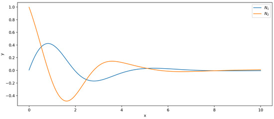
Figure 3.
PINN results for IVP (14) with final loss function value .
Then, we use PWNN to solve the problem with less training data and the same structure as PINN above on each sub-interval. Interval is divided into five equidistant sub-intervals . The neural network employed in each sub-interval consists of two hidden layers, with each hidden layer containing 20 neurons. In order to compare it with PINN, we uniformly sample 200 data points from each sub-interval as the training data. The learning rate is set to 0.01, and each neural network performed 2000 iterations. The results of training PWNNs are shown in Figure 4. The first five graphs represent the PWNNs on each interval, as well as loss function values, and the last graph is their combination .

Figure 4.
Result figures of PWNNs: the first five is with final loss function value on each sub-interval . The last one is their combination, and .
We also solve the problem using the fourth-order Runge–Kutta method to compare the results with those of using the above methods.
In Figure 5, the results obtained by using the PINN method, PWNN approach, and fourth-order Runge–Kutta method (RK4) are presented. It can be observed that the overall results of the three methods are similar. However, compared with PINN, the results of PWNN and RK4 are closer.
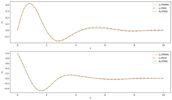
Figure 5.
Comparisons of the results of solving IVP (14) using PINN, PWNN, and RK4 methods.
It shows that PWNN is more efficient than PINN in the sense of numerical solution.
5.2. Example 2
Consider the following IVP of a SIR model of epidemic dynamics
We use PINN to find its solution over the interval . The used PINN consists of 1 input neuron, 3 hidden layers of 20 neurons each, and 3 output neuron. The 200 training points are taken from equidistantly. The network adopts Xavier initialization, employs the Adam optimization algorithm with a learning rate , and runs for 10,000 iterations. Figure 6 illustrates the solutions given by the PINN for IVP (15) over the interval . Observably, the PINN successfully computes solutions merely within the intervals (left graph) instead of large interval (right graph). That is, as the solution interval further extends the learning results of PINN notably deviate from the real case.
Figure 6.
Results of PINN to solve IVP (15) that failed to get large interval solutions.
We now solve the problem over a large interval using the PWNN method with a smaller size structure than the PINN above. Divide interval into 10 equally sized sub-intervals and Take 100 training points in each sub-interval by uniform distribution. Construct a neural network for each segment, where each network consists of 1 input neuron, 1 hidden layer with 20 neurons, and 3 output neurons. Utilize Xavier initialization and Adam optimization algorithms for each network with learning rate and 10,000 iterations to train on interval .
Figure 7 illustrates the training results of PWNNs for all sub-intervals. The titles of the figures specify the names of the networks for each interval along with the respective values of the loss function after the completion of network training. Figure 8 displays the comparisons between the results of both PWNNs and the RK4 method. The solid lines represent the solutions obtained from PWNNs, while the discrete points depict the solutions obtained using the RK4 method. Obviously, PWNN gives a large interval solution to problem (15) that is highly consistent with RK4.

Figure 7.
Results of PWNNs on for and loss function values for each PWNN.
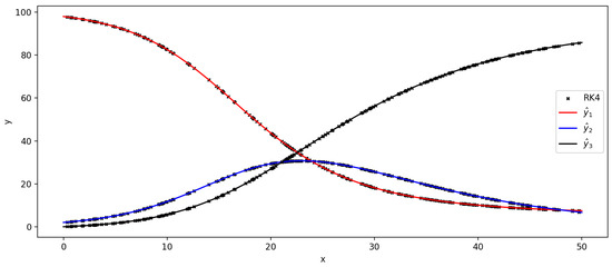
Figure 8.
Comparison of the results of using PWNN and RK4 methods.
Example 2 shows that the direct application of conventional PINN can only obtain the intercell solution (local solution) of the problem, while PWNN directly gives a large interval solution consistent with RK4, which demonstrates the effectiveness of the given PWNN algorithm.
5.3. Example 3
The Lotka–Volterra system describes the interaction between predator and prey, where the predator depends on the prey for food, and the prey is threatened by the predator. The model can be mathematically expressed as
We take , , considering initial condition , on interval [0, 20] to solve it. We first solve it with a [1, 20, 20, 2] PINN, where [1, 20, 20, 2] refers to the network having one input neuron, with two hidden layers in the middle, each with 20 neurons, and the output layer with two neurons. The network is trained for 10 rounds with 10,000 iterations in each round, the learning rate is and the optimizer is Adam. The training results are shown in the Figure 9, which shows that PINN has a large gap with the results predicted by RK4 after 10 rounds of training. Furthermore, we also attempted to separately increase the width and depth of the PINN and conduct training with the same training settings. The network’s prediction results are presented in the Figure 9, and the loss results are shown in the Table 1. It can be found that, in the broader interval [0, 20], the increase in the depth of the PINN failed to enhance the performance of the model (the loss after 10 rounds of training was not lower than that of the shallow PINN). The PINN with increased depth, although the loss was decreasing, did not have a high accuracy after 10 rounds of training.
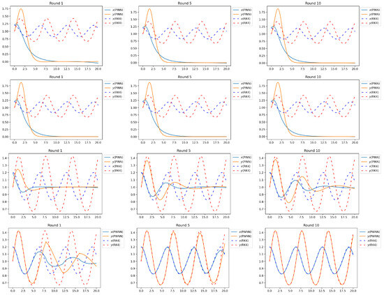
Figure 9.
Row 1 is the result of [1, 20, 20, 2] PINN, row 2 is the result of [1, 20, 20, 20, 2] PINN, row 3 is the result of [1, 50, 50, 2] PINN, and row 4 is the result of PWNN.

Table 1.
The loss value for problem (16) in PINN.
We now uniformly divide the interval into five segments, training each sub-interval with a PINN. The training configuration remains consistent with the previously described settings, with network prediction results presented in the accompanying Figure 9 and loss outcomes summarized in the Table 2. It is evident that from the first to the fifth iteration, as well as from the fifth to the tenth iteration, the loss for each sub-network shows a significant reduction, with the network predictions closely approximating those obtained using the high-accuracy RK4 method. Let us denote the parameter count of a PINN as . The parameter count for a deeper PINN is approximately , while the parameter count for a wider PINN is about . In comparison, the parameter number of PWNN with the added number of networks is . This indicates that, without increasing the overall parameter count, enhancing the number of networks is more effective than augmenting their depth or width.
Table 2.
The loss value for problem (16) in PWNN.
For a clearer comparison with the accepted traditional methods, we calculate the mean square error between each network and RK4. From the Table 3, it can be seen quantitatively that among the various networks, our proposed piecewise neural network method is the closest to the results of RK4.
Table 3.
The mean square error between the predicted results of each network and the RK4 results.
5.4. Example 4
Consider the following IVP:
As in previous examples, we first use PINN to find the numerical solutions of the problem in the interval . We perform four rounds of training for PINN, with 10,000 iterations per round. The learning rate is set to 0.001 for the first round and 0.0001 for the subsequent rounds. In these experiments, the values of the loss function remains around for different rounds. This indicates that further increasing the number of training rounds and iterations does not significantly reduce the loss function value. The training results are shown in Figure 10.
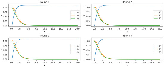
Figure 10.
PINN solutions of problem (17) in different rounds.
When using PWNN, we divide the solution interval into five equal parts and construct corresponding PWNNs. Then, train each PWNN for four rounds, with each round consisting of 10,000 iterations on each sub-interval. The learning rate for the first round of training is set to , while for the remaining rounds, it is set to . The training results of the PWNNs are shown in Figure 11.
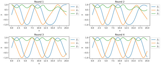
Figure 11.
PWNN solutions of IVP (17) in different rounds.
The values of the loss function corresponding to each round of PWNN are shown in Table 4. It can be observed that as the number of training rounds increases, the loss function values of the PWNNs gradually decreases. In Figure 12, we show the comparisons of results of the PWNN in the fourth round with those of RK4. It can be seen that the results of the PWNN method are in good agreement with those of the RK4 method.
Table 4.
Comparisons of the results obtained by PWNN and RK4 for solving IVP (17).

Figure 12.
Comparison of solving results of PWNN and RK4 methods for IVP (17).
6. Discussion and Conclusions
The neural network-based method for solving differential equations provides solutions with excellent generalization properties. Models based on neural networks offer opportunities to theoretically and practically tackle differential equation problems across various sciences and engineering applications, while most other techniques offer discrete solutions, solutions with limited differentiability, or strongly depend on the discrete scheme of the variable domain. Effectively using the advantages of the nonlinear approximation of artificial neural networks and overcoming the shortcomings of traditional numerical methods is a hot research direction at present.
In this paper, based on the advantages of PINN local strong convergence, we propose a piecewise neural network method for solving initial value problems of ODEs over large intervals of the independent variable. This method not only provides an approach for the coordination of multiple networks to solve an IVP of ODEs but also introduces a parameter transfer and multiple rounds of pre-training technique to effectively enhance the accuracy of network solutions in training multi-correlation ANN models. On one hand, we offer a new method to address the solution extension problem of initial value problems of differential equations. On the other hand, our work aims to contribute to both the theoretical and practical aspects of applying ANNs, providing deep insights into the application of modern methods to traditional mathematical problems.
Through comparative experiments, we prove that under almost the same network training environment, the training time of piecewise neural networks is shorter, the convergence speed to the solution to the studied problem is faster, and it can also make up for the defects of the basic ANN algorithm. Furthermore, in Section 5.2, when PINN is used to solve the Equation (15) over a large solution domain, although the final loss value obtained by PINN training is very low, the approximate solution obtained does not match the actual solution. This may be attributed to two reasons. On the one hand, it shows that the optimization of the residual loss function is only a necessary condition for the artificial neural network output to be an approximate solution to the problem, but not a sufficient condition. On the other hand, this is due to small numerical instabilities during backpropagation because of the complexity of the loss hypersurface, where the ANN can settle on a local minimum with a small value for the loss function [2]. The piecewise neural network method proposed in this paper solves these problems effectively to some extent.
Certainly, there are some limitations to this study. We have not yet compared it with some newer methods, such as in [38]. We did not consider applying the proposed method to partial differential equation problems, which would involve partitioning high-dimensional domains of independent variables. The successful application of this method strongly depends on the effective training of sub-neural networks on each corresponding interval. In other words, if an ANN in a certain link cannot be effectively trained in the training of a PWNN, the whole algorithm may not complete the solving task. Furthermore, the continuity and differentiability of network solution over the entire interval have yet to be guaranteed theoretically. These are topics for further study in the future.
Author Contributions
C.T. played a key role in conceptualizing the project, developing the methodology, providing supervision throughout the process, and contributing to writing, reviewing, and editing the content. D.H. was responsible for programming, result validation, and visualization tasks and contributed to the preparation of the original draft through writing. Both authors made significant contributions to the project, ensuring its accuracy and quality. All authors have read and agreed to the published version of the manuscript.
Funding
This project is supported by the National Natural Science Foundation of China (no.11571008).
Data Availability Statement
No new data were created or analyzed in this study. Data sharing is not applicable to this article.
Acknowledgments
The authors would like to thank the editor and reviewers for their valuable suggestions and comments.
Conflicts of Interest
The authors declare no conflicts of interest.
References
- Braun, M. Differential Equations and Their Applications; Springer: Berlin/Heidelberg, Germany, 1993. [Google Scholar]
- Piscopo, M.L.; Spannowsky, M.; Waite, P. Solving differential equations with neural networks: Applications to the calculation of cosmological phase transitions. Phys. Rev. D. 2019, 100, 016002. [Google Scholar] [CrossRef]
- Yadav, N.; Yadav, A.; Kumar, M. An Introduction to Neural Network Methods for Differential Equations; Springer: Berlin/Heidelberg, Germany, 2015; pp. 43–100. [Google Scholar]
- Hornik, K.; Stinchcombe, M.; White, H. Multilayer feedforward networks are universal approximators. Neural Netw. 1989, 2, 359–366. [Google Scholar] [CrossRef]
- Kurt, H.; Maxwell, S.; Halbert, W. Universal approximation of an unknown mapping and its derivatives using multilayer feedforward networks. Neural Netw. 1990, 3, 551–560. [Google Scholar] [CrossRef]
- Li, X. Simultaneous approximations of multivariate functions and their derivatives by neural networks with one hidden layer. Neurocomputing 1996, 12, 327–343. [Google Scholar] [CrossRef]
- Lagaris, I.E.; Likas, A.; Fotiadis, D.I. Artificial neural networks for solving ordinary and partial differential equations. IEEE Trans. Neural Netw. 1998, 9, 987–1000. [Google Scholar] [CrossRef]
- Paszke, A.; Gross, S.; Massa, F.; Lerer, A.; Bradbury, J.; Chanan, G.; Killeen, T.; Lin, Z.; Gimelshein, N.; Antiga, L.; et al. PyTorch: An Imperative Style, High-Performance Deep Learning Library. In Proceedings of the 33rd International Conference on Neural Information Processing Systems, Vancouver, BC, Canada, 8–14 December 2019; Curran Associates Inc.: Red Hook, NY, USA, 2019; p. 12. [Google Scholar] [CrossRef]
- Louis, B.R. Automatic Differentiation: Techniques and Applications. In Lecture Notes in Computer Science; Springer: Berlin/Heidelberg, Germany, 1981. [Google Scholar]
- Arun, V. An introduction to automatic differentiation. Curr. Sci. 2000, 78, 804–807. [Google Scholar]
- Atilim, G.B.; Barak, A.P.; Alexey, A.R.; Jeffrey, M.S. Automatic Differentiation in Machine Learning: A Survey. J. Mach. Learn. Res. 2018, 18, 1–43. [Google Scholar]
- Justin, S.; Konstantinos, S. DGM: A deep learning algorithm for solving partial differential equations. J. Comput. Phys. 2018, 375, 1339–1364. [Google Scholar] [CrossRef]
- Anitescu, C.; Atroshchenko, E.; Alajlan, N.; Rabczuk, T. Artificial Neural Network Methods for the Solution of Second Order Boundary Value Problems. Comput. Mater. Contin. 2019, 59, 345–359. [Google Scholar] [CrossRef]
- Raissi, M.; Perdikaris, P.; Karniadakis, G.E. Physics-informed neural networks: A deep learning framework for solving forward and inverse problems involving nonlinear partial differential equations. J. Comput. Phys. 2019, 378, 686–707. [Google Scholar] [CrossRef]
- Yuan, L.; Ni, Y.-Q.; Deng, X.-Y.; Hao, S. A-PINN: Auxiliary physics informed neural networks for forward and inverse problems of nonlinear integro-differential equations. J. Comput. Phys. 2022, 462, 111260. [Google Scholar] [CrossRef]
- Chiu, P.-H.; Wong, J.C.; Ooi, C.; Dao, M.H.; Ong, Y.-S. CAN-PINN: A fast physics-informed neural network based on coupled-automatic–numerical differentiation method. Comput. Methods Appl. Mech. Eng. 2022, 395, 114909. [Google Scholar] [CrossRef]
- Huang, Y.; Hao, W.; Lin, G. HomPINNs: Homotopy physics-informed neural networks for learning multiple solutions of nonlinear elliptic differential equations. Comput. & Math. Appl. 2022, 121, 62–73. [Google Scholar] [CrossRef]
- Fang, Y.; Wu, G.-Z.; Wang, Y.-Y.; Dai, C.-Q. Data-driven femtosecond optical soliton excitations and parameters discovery of the high-order NLSE using the PINN. Nonlinear Dyn. 2021, 105, 603–616. [Google Scholar] [CrossRef]
- Bai, Y.; Chaolu, T.; Bilige, S. The application of improved physics-informed neural network (IPINN) method in finance. Nonlinear Dyn. 2022, 107, 3655–3667. [Google Scholar] [CrossRef]
- Meng, X.; Li, Z.; Zhang, D.; Karniadakis, G.E. PPINN: Parareal physics-informed neural network for time-dependent PDEs. Comput. Methods Appl. Mech. Eng. 2020, 370, 113250. [Google Scholar] [CrossRef]
- Long, Z.; Lu, Y.; Dong, B. PDE-Net 2.0: Learning PDEs from data with a numeric-symbolic hybrid deep network. J. Comput. Phys. 2019, 399, 108925. [Google Scholar] [CrossRef]
- Zha, W.; Zhang, W.; Li, D.; Xing, Y.; He, L.; Tan, J. Convolution-Based Model-Solving Method for Three-Dimensional, Unsteady, Partial Differential Equations. Neural Comput. 2022, 34, 518–540. [Google Scholar] [CrossRef]
- Han, G.; Luning, S.; Jian-Xun, W. PhyGeoNet: Physics-informed geometry-adaptive convolutional neural networks for solving parameterized steady-state PDEs on irregular domain. J. Comput. Phys. 2021, 428, 110079. [Google Scholar] [CrossRef]
- Wang, N.; Zhang, D.; Chang, H.; Li, H. Deep learning of subsurface flow via theory-guided neural network. J. Hydrol. 2020, 584, 124700. [Google Scholar] [CrossRef]
- Wang, N.; Chang, H.; Zhang, D. Theory-guided Auto-Encoder for surrogate construction and inverse modeling. Comput. Methods Appl. Mech. Eng. 2021, 385, 114037. [Google Scholar] [CrossRef]
- Zhang, R.-F.; Bilige, S. Bilinear neural network method to obtain the exact analytical solutions of nonlinear partial differential equations and its application to p-gBKP equation. Nonlinear Dyn. 2019, 95, 3041–3048. [Google Scholar] [CrossRef]
- Zhang, R.; Bilige, S.; Chaolu, T. Fractal Solitons, Arbitrary Function Solutions, Exact Periodic Wave and Breathers for a Nonlinear Partial Differential Equation by Using Bilinear Neural Network Method. J. Syst. Sci. Complex. 2021, 34, 122–139. [Google Scholar] [CrossRef]
- Yu, C.C.; Tang, Y.C.; Liu, B.D. An adaptive activation function for multilayer feedforward neural networks. In Proceedings of the 2002 IEEE Region 10 Conference on Computers, Communications, Control and Power Engineering, TENCOM ’02. Proceedings. Beijing, China, 28–31 October 2002; IEEE: Piscataway, NJ, USA, 2002; pp. 645–650. [Google Scholar]
- Dushkoff, M.; Ptucha, R. Adaptive Activation Functions for Deep Networks. Electron. Imaging 2016, 28, 1–5. [Google Scholar] [CrossRef]
- Qian, S.; Liu, H.; Liu, C.; Wu, S.; Wong, H.S. Adaptive activation functions in convolutional neural networks. Neurocomputing 2018, 272, 204–212. [Google Scholar] [CrossRef]
- Wang, S.; Yu, X.; Perdikaris, P. When and why PINNs fail to train: A neural tangent kernel perspective. J. Comput. Phys. 2022, 449, 110768. [Google Scholar] [CrossRef]
- Xiang, Z.; Peng, W.; Liu, X.; Yao, W. Self-adaptive loss balanced Physics-informed neural networks. Neurocomputing 2022, 496, 11–34. [Google Scholar] [CrossRef]
- Jagtap, A.D.; Kawaguchi, K.; Karniadakis George, E. Adaptive activation functions accelerate convergence in deep and physics-informed neural networks. J. Comput. Phys. 2020, 404, 109136. [Google Scholar] [CrossRef]
- Wen, Y.; Chaolu, T. Learning the Nonlinear Solitary Wave Solution of the Korteweg–De Vries Equation with Novel Neural Network Algorithm. Entropy 2023, 25, 704. [Google Scholar] [CrossRef]
- Wen, Y.; Chaolu, T. Study of Burgers–Huxley Equation Using Neural Network Method. Axioms 2023, 12, 429. [Google Scholar] [CrossRef]
- Wen, Y.; Chaolu, T.; Wang, X. Solving the initial value problem of ordinary differential equations by Lie group based neural network method. PLoS ONE 2022, 17, e0265992. [Google Scholar] [CrossRef] [PubMed]
- Ying, W.; Temuer, C. Lie Group-Based Neural Networks for Nonlinear Dynamics. Int. J. Bifurc. Chaos 2023, 33, 2350161. [Google Scholar] [CrossRef]
- Fabiani, G.; Galaris, E.; Russo, L.; Siettos, C. Parsimonious Physics-Informed Random Projection Neural Networks for Initial Value Problems of ODEs and Index-1 DAEs. Chaos Interdiscip. J. Nonlinear Sci. 2023, 33, 043128. [Google Scholar] [CrossRef] [PubMed]
- Glorot, X.; Bengio, Y. Understanding the difficulty of training deep feedforward neural networks. J. Mach. Learn. Res.-Proc. Track 2010, 9, 249–256. [Google Scholar]
- Kingma, D.P.; Ba, J. Adam: A Method for Stochastic Optimization. arXiv 2017, arXiv:1412.6980. [Google Scholar] [CrossRef]
Disclaimer/Publisher’s Note: The statements, opinions and data contained in all publications are solely those of the individual author(s) and contributor(s) and not of MDPI and/or the editor(s). MDPI and/or the editor(s) disclaim responsibility for any injury to people or property resulting from any ideas, methods, instructions or products referred to in the content. |
© 2024 by the authors. Licensee MDPI, Basel, Switzerland. This article is an open access article distributed under the terms and conditions of the Creative Commons Attribution (CC BY) license (https://creativecommons.org/licenses/by/4.0/).