A Novel Two-Lane Lattice Model Considering the Synergistic Effects of Drivers’ Smooth Driving and Aggressive Lane-Changing Behaviors

Abstract

Most existing two-lane traffic flow lattice models fail to fully consider the interactions between drivers’ aggressive lane-changing behaviors and their desire for smooth driving, as well as their combined effects on traffic dynamics. To fill this research gap, under symmetric lane-changing rules, this paper proposes a novel two-lane lattice model that incorporates these two factors as co-influencers. Based on linear and nonlinear stability analyses, we derive the linear stability conditions of the new model, along with the density wave equation and its solutions describing traffic congestion propagation near critical points. Numerical simulations validate the theoretical findings. The results indicate that in the two-lane framework, enhancing either drivers’ lane-changing aggressiveness or introducing the desire for smooth driving alone can somewhat improve traffic flow stability. However, when considering their synergistic effects, traffic flow stability is enhanced more significantly, and the traffic congestion is suppressed more effectively.

1. Introduction

Currently, macroscopic and microscopic models have emerged as two typical traffic flow models for studying the mechanisms of traffic congestion. Macroscopic traffic flow models primarily aim to reveal the spatiotemporal evolution patterns of overall traffic flow and typically include lattice models [1,2,3] and continuous models [4,5,6]. Microscopic traffic flow models, on the other hand, focus on elucidating the movement patterns of individual vehicles within road systems, mainly including cellular automaton models [7,8,9] and car-following models [10,11,12,13]. Among these traffic flow models, lattice models have garnered significant attention from scholars due to their integration of the advantages of both macroscopic and microscopic models, as well as their convenience in deriving density wave equations that describe the propagation of traffic congestion. In 1998, Nagatani [1] pioneered a lattice model suitable for describing the operational laws of single-lane macroscopic traffic flow and successfully uncovered the propagation and evolution of traffic congestion near critical points. Subsequently, to align the lattice model closer to real-world traffic conditions, Nagatani [2] extended the original single-lane lattice model to a two-lane framework by introducing lane-changing rules. However, due to oversimplified assumptions, the model has limitations in simulating complex traffic environments. To precisely reproduce and simulate the nonlinear phenomena of complex traffic systems at a higher level, subsequent researchers have conducted a series of extensions based on Nagatani’s single-lane or two-lane frameworks. By incorporating various influencing factors such as driver anticipation effects [14,15,16,17], traffic jerk effects [18], overtaking on curves effects [19,20], honking effects [21,22], and backward-looking effects [23,24,25], they have successfully constructed a series of lattice models that are more aligned with actual traffic conditions. These models not only provide powerful tools for the study of traffic flow theory but also offer important references for practical traffic management and planning.

In two-lane systems, the lane-changing behavior plays a pivotal role in reducing congestion and optimizing traffic flow. However, traditional two-lane lattice models assume lane changes occur when the lateral space on the neighboring lane is slightly larger than the headway on the current lane, ignoring safety distance requirements. In reality, within actual road environments, drivers consider multiple factors when deciding whether to change lanes. Especially when the lateral space in the adjacent lane is only marginally larger than the headway in the current lane, they often refrain from lane changes for safety reasons. Addressing this deficiency, Li et al. [26] proposed a more realistic lane-changing rule, which emphasizes that lane changes should occur based on the condition that the lateral space in the target lane is significantly greater than the headway in the current lane, sometimes even requiring this space to be multiple times the headway, thereby ensuring the safety of lane-changing operations. Simultaneously, they innovatively introduced a parameter to describe the level of aggressiveness in drivers’ lane-changing decisions, which we refer to as aggressive lane-changing behaviors. This parameter precisely characterizes the risk preferences of different drivers by quantifying the multiple relationship between the headway of the current vehicle and its lateral distance. The research results indicate that this improved lane-changing assumption not only enhances the model’s ability to explain actual traffic behavior but also reveals the profound impact of drivers’ lane-changing aggressiveness on the stability of traffic flow in two-lane systems.

In addition, current research [27,28,29] has confirmed that in real-world driving scenarios, apart from the influence of traffic conditions ahead on the operational state of the current vehicle, drivers’ desires for smooth driving, characterized by the difference between desired and actual speed, also affect the dynamic behavior of vehicles. In actual vehicle control, drivers flexibly adjust their driving strategies based on real-time road conditions, striving to achieve smooth driving to reduce energy losses and passenger discomfort resulting from rapid acceleration and deceleration. Despite the non-negligible impact of drivers’ smooth driving desires on the performance of transportation systems, this crucial factor has received relatively limited attention in two-lane system research. Especially after introducing the innovative lane-changing mechanism that considers drivers’ lane-changing aggressiveness, the mechanism of how drivers’ smooth driving desires and lane-changing aggressiveness jointly affect the traffic dynamics in a two-lane system remains unclear. Therefore, constructing a two-lane model that can accurately simulate the combined effects of drivers’ smooth driving desires and their lane-changing behaviors on actual traffic flow is of great significance for more closely approximating real-world driving scenarios, deepening our understanding of the interaction between these two factors, and comprehensively revealing the complex dynamic nature of two-lane systems.

However, to our knowledge, there is currently a lack of literature exploring how drivers’ desires for smooth driving and their lane-changing behaviors jointly influence the traffic dynamics of two-lane systems. To fill this research gap, this paper proposes a novel two-lane lattice model that integrates the combined effects of drivers’ smooth driving desires and aggressive lane-changing behaviors within the theoretical framework of lattice models. Subsequently, an in-depth theoretical analysis and numerical simulation study of the proposed model are conducted to reveal the synergistic effects of drivers’ smooth driving and aggressive lane-changing behaviors on traffic flow in a two-lane system. The objective of this innovative work is to more accurately simulate and analyze the synergistic effect between drivers’ smooth driving desires and their lane-changing behaviors in real-world traffic, aiming to provide an effective analytical model that allows us to precisely understand and grasp the evolution patterns of macroscopic traffic flow in a two-lane system. Compared with previous research results, this paper provides a more profound insight into the synergistic effects between drivers’ aggressive lane-changing behaviors and their desire for smooth driving, emphasizing its positive role in enhancing the stability of two-lane systems and improving traffic operational efficiency.

The structure of the paper is as follows: A novel two-lane lattice model that takes into account the combined effects of drivers’ aggressive lane-changing and smooth driving is presented in Section 2. In Section 3, criteria for stabilizing traffic flow in two-lane systems are derived through linear stability analysis. To gain a better understanding of traffic congestion in two-lane systems, Section 4 presents nonlinear analysis and derives the mKdV density wave equation. Numerical simulations are presented in Section 5 to validate the theoretical findings from Section 3 and Section 4. The main findings are finally summed up in Section 6.

2. Models

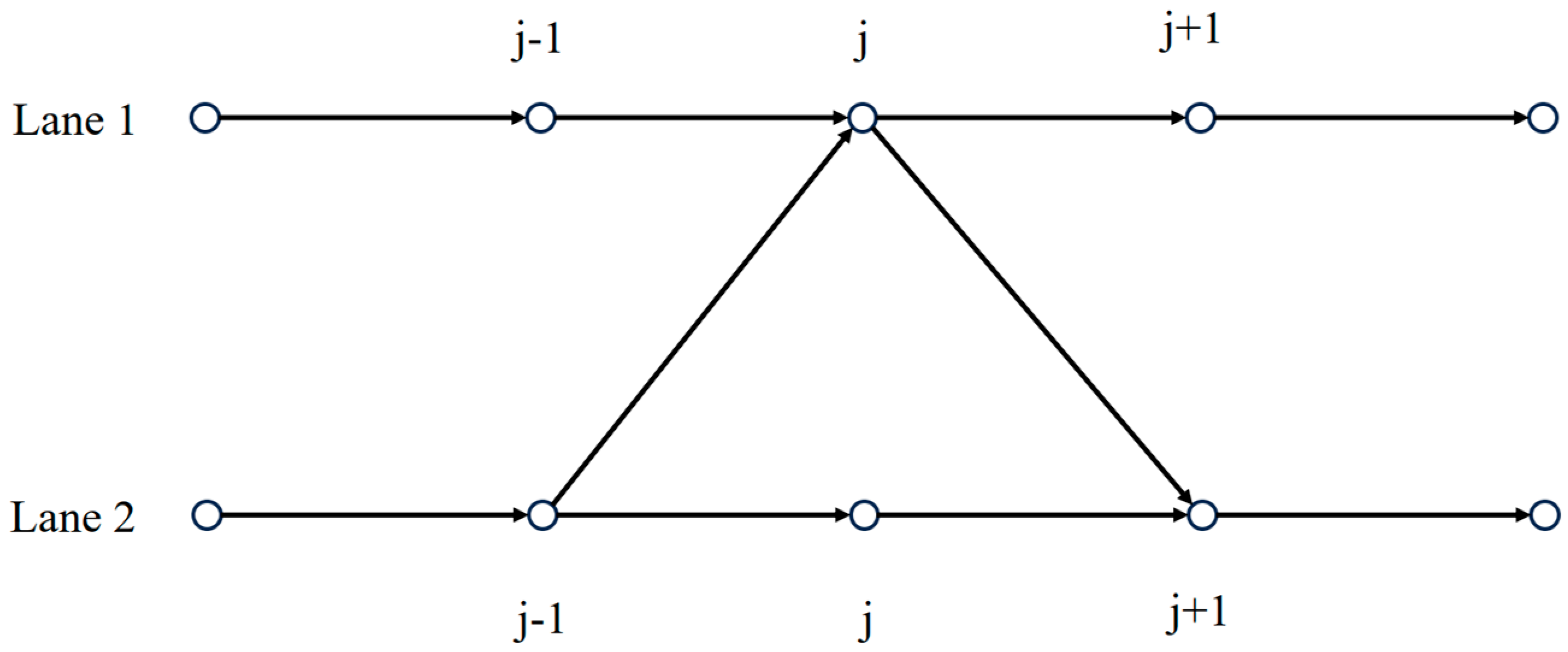
A schematic diagram of the operation of the traffic flow for a two-lane highway system is given in Figure 1. In this two-lane system, vehicles are free to change lanes between the two lanes. Since all lanes are homogeneous, the probability of a vehicle changing lanes between the two is equal. This lane-changing rule is referred to as the symmetric lane-changing rule. To describe the dynamic behavior of the traffic flow within the symmetric lane-changing rule depicted in Figure 1, in 1999, Nagatani [2] proposed the following lattice traffic flow model:

$${\partial }_t{\rho }_j(t)+{\rho }_0\left({\rho }_j(t)v_j(t)-{\rho }_{j-1}(t)v_{j-1}(t)\right)=\gamma \left|{\rho }_0^2{V}^{\prime }\left({\rho }_0\right)\right|\left({\rho }_{j+1}(t)-2{\rho }_j(t)+{\rho }_{j-1}(t)\right)$$

(1)

$${\partial }_t({\rho }_j{v}_j)=a[{\rho }_{0}V({\rho }_{j+1})-{\rho }_j{v}_j]$$

(2)

in which the variables ${\rho }_j\left(t\right)$ and $v_j\left(t\right)$ represent the local density and local velocity of the $j\mathrm{th}$ lattice site at time t, respectively. ${\rho }_0$ is the total average density of the traffic system. The constant $\gamma$ represents the lane-changing coefficient. The term $\gamma \left|{\rho }_0^2{V}^{\prime }\left({\rho }_0\right)\right|$ is introduced mainly for the dimensionless treatment of the conservation equations. Parameter $a$ represents the driver’s sensitivity coefficient. In the Nagatani two-lane lattice model, Equation (1) represents the conservation equation, while Equation (2) denotes the vehicle motion equation.

$V\left(\rho \right)$ is the optimized velocity function, which is expressed as follows [30]:

$$V({\rho }_j)=\tanh ({\displaystyle \frac{2}{{\rho }_0}}-{\displaystyle \frac{{\rho }_j(t)}{{\rho }_0^2}}-{\displaystyle \frac{1}{{\rho }_c}})+\tanh ({\displaystyle \frac{1}{{\rho }_c}})$$

(3)

where ${\rho }_c$ is the critical density. As ${\rho }_0={\rho }_c$, the optimized velocity function $V\left(\rho \right)$ has an inflection point at ${\rho }_j={\rho }_c$.

Based on the original Nagatani two-lane lattice model, researchers have developed a series of enhanced models by incorporating factors that better align with real-world conditions. In the original Nagatani two-lane lattice model and its subsequent improved versions [15,19,31,32,33,34], a common assumption for the lane-changing rule is that a vehicle will change lanes if the distance to the leading vehicle in its current lane (headway) was less than the distance to the leading vehicle in the adjacent lane (lateral distance). However, this lane-changing assumption ignores the need for a safe distance required to avoid inter-vehicle collisions during the lane-changing process, and thus these two-lane lattice models do not exactly match the rules of operation of actual two-lane systems. Recently, a more logical and practical modification to the lane-changing hypothesis has emerged: only when the lateral distance of the considered vehicle is significantly greater than its headway, the driver will perform the lane-changing operation under the premise of ensuring safety. Guided by this refined lane-changing assumption, Li et al. [26] have reconstructed the lane-changing rule for the two-lane system and derived a new conservation equation accordingly. Specifically, their modeling framework postulates that if the density of vehicles at site j − 1 on lane 2 exceeds $f$ times the density at site j on lane 1, then vehicles from lane 2 will switch to lane 1 with lane-changing flow rate $\gamma \left|{\rho }_0^2{V}^{\prime }\left({\rho }_0\right)\right|\left({\rho }_{2,j-1}-f{\rho }_{1,j}\right)$. Similarly, when the density of site $j$ on lane 1 is $f$ times higher than the density of site $j+1$ on lane 2, lane-changing behavior will occur, and the resulting lane-changing flow rate is $\gamma \left|{\rho }_0^2{V}^{\prime }\left({\rho }_0\right)\right|\left({\rho }_{1,j}-f{\rho }_{2,j+1}\right)$. Hence the conservation equation for lane 1 in the two-lane system under the refined lane-changing assumption is

$$\begin{array}{r}{\partial }_t{\rho }_{1,j}(t)+{\rho }_0({\rho }_{1,j}(t)v_{1,j}(t)-{\rho }_{1,j-1}(t)v_{1,j-1}(t))=\gamma |{\rho }_0^2{V}^{\prime }({\rho }_0)|[f{\rho }_{2,j-1}\\ -(1+f){\rho }_{1,j}+{\rho }_{2,j+1}]\end{array}$$

(4)

Similarly, lane 2 has conservation equations as follows:

$$\begin{array}{r}{\partial }_t{\rho }_{2,j}(t)+{\rho }_0({\rho }_{2,j}(t)v_{2,j}(t)-{\rho }_{2,j-1}(t)v_{2,j-1}(t))=\gamma |{\rho }_0^2{V}^{\prime }({\rho }_0)|[f{\rho }_{1,j-1}\\ -(1+f){\rho }_{2,j}+{\rho }_{1,j+1}]\end{array}$$

(5)

where ${\rho }_{k,j}$ and $v_{k,j}$ represents the density and velocity of $k\mathrm{th}$ ($k=1,2$) lane at site $j$, respectively.

To simplify the subsequent analysis, we add Equations (4) and (5) together, resulting in a new conservation equation for the two-lane lattice model [26].

$${\partial }_t{\rho }_j+{\rho }_0({\rho }_j{v}_j-{\rho }_{j-1}{v}_{j-1})=\gamma |{\rho }_0^2{V}^{\prime }({\rho }_0)|[{\rho }_{j-1}+f{\rho }_{j+1}-(f+1){\rho }_j]$$

(6)

where ${\rho }_j=\left({\rho }_{1,j}+{\rho }_{2,j}\right)/2$,${\rho }_j{v}_j=\left({\rho }_{1,j}{v}_{1,j}+{\rho }_{2,j}{v}_{2,j}\right)/2$.

It should be emphasized that in the two-lane system, the lateral distance and headway distance of the considered vehicle are the key factors that determine the driver’s lane-changing behavior. The proportional relationship $f$ between these two factors directly reflects the aggressiveness of the driver’s lane-changing behavior. Specifically, for a given local vehicle density (i.e., headway distance) of the current lane, a smaller value of $f$ indicates a higher local density in the target lane, where the driver requires less lateral space for lane changing, demonstrating a more aggressive lane-changing behavior. Conversely, a larger f indicates a more conservative lane-changing behavior. Therefore, the parameter f is an effective indicator for assessing the aggressiveness of lane-changing behavior in the two-lane system, and the aggressiveness is inversely proportional to this value.

Recently, studies in references [27,28,29] have shown that drivers’ desire to drive smoothly significantly contributes to the stability of traffic flow. However, this crucial factor has yet to be investigated in the context of two-lane traffic systems. Specifically, under complex scenarios involving aggressive lane-changing behaviors by drivers, the mechanism by which drivers’ willingness to drive smoothly affects the macroscopic evolution of traffic flow in two-lane systems remains unclear. To fill this research gap, we have incorporated the effect of drivers’ desire to drive smoothly into Equation (4), thereby deriving a new motion equation for the two-lane lattice model as follows,

$${\partial }_t({\rho }_j{v}_j)=a[{\rho }_{0}V({\rho }_{j+1})-{\rho }_j{v}_j]+\lambda {\rho }_0[V({\rho }_0)-V({\rho }_j)]$$

(7)

where $\lambda$ is the response coefficient to drivers’ desire to drive smoothly. $a=1/\tau$ represents the driver’s sensitivity coefficient, where $\tau$ denotes the delay time. Term ${\rho }_0\left[V\left({\rho }_0\right)-V\left({\rho }_j\right)\right]$ describes the driver’s willingness to pursue smooth driving in a two-lane system, where they dynamically adjust their vehicle speeds in response to the discrepancy between the current traffic flow velocity $V\left({\rho }_j\right)$ and the optimal steady-state velocity $V\left({\rho }_0\right)$. Specifically, if the vehicle speed $V\left({\rho }_j\right)$ exceeds the steady-state velocity, the driver will actively decelerate the vehicle in an attempt to approximate and maintain this ideal steady state. Conversely, when the vehicle velocity $V\left({\rho }_j\right)$ is below the steady-state velocity, acceleration measures will be taken to ensure that the vehicle velocity stabilizes around the steady-state velocity, thereby ensuring smooth traffic flow operation. Since then, composed of Equations (6) and (7), we have derived a novel two-lane lattice model that integrates the driver’s desire for smooth driving with the combined influence of aggressive lane-changing behaviors.

In particular, when the parameter $f=1$ and $\lambda =0$, the new model reduces to the classical Nagatani two-lane lattice model, signifying that the original Nagatani two-lane lattice model [2] is a special case within our proposed framework.

In the presented model, the driver’s perceptual ability [35] is described based on the time required for the driver to perceive the stimulus of deviation information (such as the discrepancy between the current traffic flow velocity and the optimal steady-state velocity) and adjust his or her speed accordingly. Thus, the parameters $a$ and $\lambda$ characterize the driver’s sensitivity and responsiveness to external stimuli or changes in traffic conditions. According to the literature [36], the sensitivity coefficient and response coefficient of drivers are closely related to factors such as driver categories and different driving environments, exhibiting significant heterogeneity. However, to simplify this study, we assume that the sensitivity coefficient and response coefficient of drivers are constant.

Eliminating the velocity variables in Equations (6) and (7), the evolution equation of traffic flow density in the two-lane scenario can be obtained as follows:

$$\begin{array}{l}{\rho }_j(t+2\tau )-{\rho }_j(t+\tau )+\tau {\rho }_0^2[(V({\rho }_{j+1}(t))-V({\rho }_j(t)))]-\tau k{\rho }_0^2[V({\rho }_j(t))-V({\rho }_{j-1}(t))]\\ -\gamma \tau \left|{\rho }_0^2{V}^{\prime }({\rho }_0)\right|[{\rho }_{j-1}(t+\tau )+f{\rho }_{j+1}(t+\tau )-(f+1){\rho }_j(t+\tau )]=0\end{array}$$

(8)

where $\lambda =k/\tau$.

3. Linear Stability Analysis

The steady-state solution of the density evolution Equation (8) in the two-way system is as follows:

$${\rho }_j(t)={\rho }_0, v_j(t)=V({\rho }_0)$$

(9)

Applying a small disturbance signal $y_j\left(t\right)$ to the steady-state solution, we have the following formula

$${\rho }_j(t)={\rho }_0+y_j(t)$$

(10)

Substituting Equation (10) into the density evolution Equation (8) and linearizing the equation can be obtained as follows:

$$\begin{array}{l}{y}_j(t+2\tau )-y_j(t+\tau )-\tau \gamma \left|{\rho }_0^2{V}^{\prime }({\rho }_0)\right|[y_{j-1}(t+\tau )+f{y}_{j+1}(t+\tau )\\ -(f+1)y_j(t+\tau )]+\tau {\rho }_0^2{V}^{\prime }({\rho }_0)[y_{j+1}(t)-y_j(t)]\\ +\tau k{\rho }_0^2{V}^{\prime }({\rho }_0)[y_{j-1}(t)-y_j(t)]=0\end{array}$$

(11)

where $V^{\prime }\left({\rho }_0\right)=\left[{\displaystyle \frac{dV\left({\rho }_j\right)}{d}}{\rho }_j\right]{|}_{{\rho }_j={\rho }_0}$. Expanding $y_j\left(t\right)$ in Equation (11) as a Fourier series form: $y_j\left(t\right)=\mathit{exp}(ikj+zt)$, one can obtain:

$$\begin{array}{l}{e}^{2\tau z}-e^{\tau z}+\tau {\rho }_0^2{V}^{\prime }({\rho }_0)(e^{ik}-1)+\tau k{\rho }_0^2{V}^{\prime }({\rho }_0)(e^{-ik}-1)\\ -\tau \gamma \left|{\rho }_0^2{V}^{\prime }({\rho }_0)\right|(e^{-ik}-(f+1)+f{e}^{ik})e^{\tau z}=0\end{array}$$

(12)

To obtain the first- and second-order terms with respect to parameter $ik$, the variable $z$ in Equation (12) is expanded into the form $z=z_{1}ik+z_2{(ik)}^2+\cdots$, from which we obtain

$$z_1=(f-1)\gamma \left|{\rho }_0^2{V}^{\prime }({\rho }_0)\right|+(k-1){\rho }_0^2{V}^{\prime }({\rho }_0)$$

(13)

$$\begin{array}{c}{z}_2=-{\displaystyle \frac{3\tau z_1^2}{2}}-{\displaystyle \frac{1+k}{2}}{\rho }_0^2{V}^{\prime }({\rho }_0)+{\displaystyle \frac{1}{2}}\gamma (1+f)\left|{\rho }_0^2{V}^{\prime }({\rho }_0)\right|\\ +\gamma (f-1)\left|{\rho }_0^2{V}^{\prime }({\rho }_0)\right|\tau z_1\end{array}$$

(14)

Based on the analytical framework of the long-wave expansion method, if $z_2<0$, it indicates that small perturbation signals will gradually amplify over time, leading to intensified traffic flow fluctuations and a tendency towards instability. Conversely, if $z_2>0$, it suggests that the two-lane system possesses an inherent self-regulating mechanism, where small perturbation signals are gradually absorbed and effectively suppressed, ultimately resulting in a stable traffic flow state. From this, we can derive the critical stability condition for the new model as follows:

$$\tau =-{\displaystyle \frac{1+k+(1+f)\gamma }{[3(1-k)+(f-1)\gamma ][1-k+(f-1)\gamma ]{\rho }_0^2{V}^{\prime }({\rho }_0)}}$$

(15)

The criterion for maintaining stability in two-lane highway traffic flow lattice model is:

$$\tau <-{\displaystyle \frac{1+k+(1+f)\gamma }{[3(1-k)+(f-1)\gamma ][1-k+(f-1)\gamma ]{\rho }_0^2{V}^{\prime }({\rho }_0)}}$$

(16)

In particular, when $f=1$,$k=0$ the stability conditions of the proposed model degenerate into stability conditions consistent with Nagatani’s two-lane lattice model [2] as follows:

$$\tau <-{\displaystyle \frac{1+2\gamma }{3{\rho }_0^2{V}^{\prime }({\rho }_0)}}$$

(17)

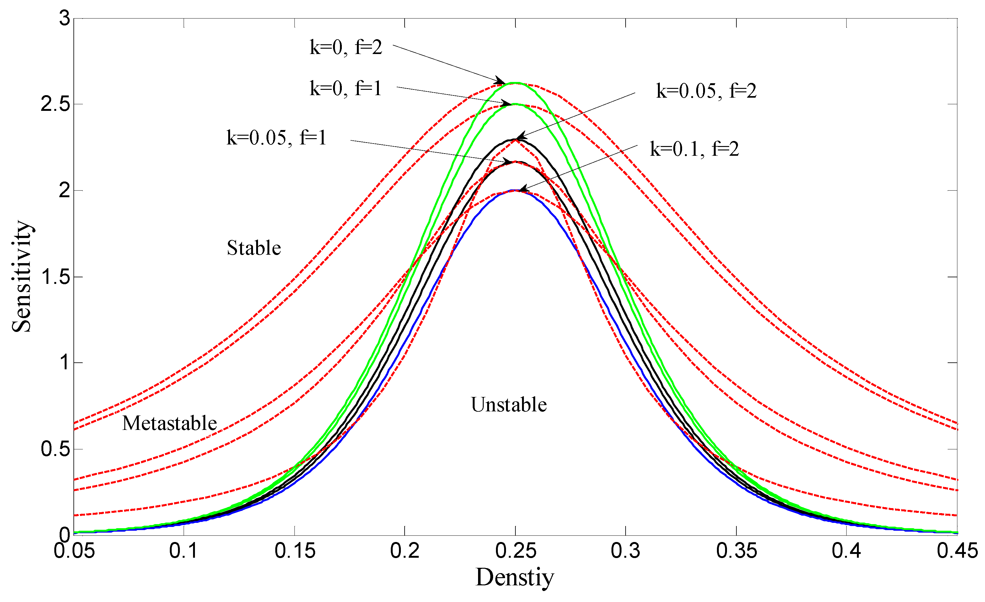
Based on the critical stability condition Equation (15), Figure 2 illustrates the critical stability curves of the new model under different combinations of the lane change adjustment intensity coefficient (LCAIC) $f$ and the reaction coefficient $k$, where the input parameter set $\gamma =0.1$. In Figure 2, the solid line depicts the neutral stability curve, while the dashed line represents the coexistence curve obtained through nonlinear analysis (discussed in detail in Section 4). Each pair of dashed and solid lines jointly divides the phase space into three regions: the stable region, the metastable region, and the unstable region. In the stable region, initially uniformly distributed traffic flow at a constant speed will, when subjected to small disturbances, see these disturbances gradually diminish over time and eventually disappear, allowing the traffic flow to revert to a stable state. However, in the metastable and unstable regions, when uniform traffic flow is perturbed slightly, these disturbances will gradually spread and amplify, ultimately leading to the stop-and-go traffic congestion phenomenon. Furthermore, it is noteworthy that on each curve in Figure 2, there exists a vertex, referred to as the critical stability point, with coordinates $\left({\rho }_c,a_c\right)$.

From Figure 2, we can find that the stability of traffic flow in the two-lane system is closely related to the values of the parameter $f$ and $k$. The following conclusions can be drawn from Figure 2:

(1) When the parameter f is fixed (for instance, at 1 or 2), the stable region in the phase diagram expands as the parameter k increases, indicating that drivers’ desire for smooth driving has a positive impact on the stability of traffic flow in the two-lane system. (2) When the parameter k is fixed (for example, at 0 or 0.05), the stability of traffic flow in the two-lane system enhances as the LCAIC parameter $f$ decreases, suggesting that in a two-lane system, drivers adopting proactive lane-changing strategies can effectively improve the stability of traffic flow. (3) Among the parameter combinations, when $k$ = 0.05 and f = 1, the corresponding curve exhibits a broader stable region compared to when $k$ = 0, $f$ = 1, and $k$ = 0, $f$ = 2. This phenomenon reveals that taking into account the synergistic effect between aggressive lane-changing behavior and the desire for smooth driving has a more pronounced effect on enhancing the stability of traffic flow in the two-lane system than considering either of these factors alone. This finding highlights the practical value and importance of the synergistic effect of these two factors in mitigating traffic congestion.

4. Nonlinear Analysis

In this section, we will examine how traffic flow evolves in the vicinity of a two-lane highway system’s critical stable point $\left({\rho }_c,a_c\right)$ using nonlinear analysis. To this end, we introduce the slow variables as follows:

$$X=\epsilon (j+bt), T={\epsilon }^{3}t,0<\epsilon \le 1$$

(18)

where parameter b is an undetermined quantity, and the parameters $j$ and $t$, respectively, represent the spatial and temporal variables. Let the density ${\rho }_j\left(t\right)$ satisfy the following equation.

$${\rho }_j(t)={\rho }_c+\epsilon R(X,T)$$

(19)

After carrying out a Taylor expansion up to the order of ${\epsilon }^5$ and substituting Equations (18) and (19) into Equation (8), the partial differential equation can be obtained as follows:

$$\begin{array}{l}{\epsilon }^2\{b+[1-k+\gamma (f-1)]{\rho }_c^2{V}^{\prime }\}{\partial }_{X}R+{\epsilon }^3\{{\displaystyle \frac{3}{2}}{b}^2\tau +{\displaystyle \frac{1}{2}}(1+k){\rho }_c^2{V}^{\prime }\\ +{\displaystyle \frac{1}{2}}\gamma {\rho }_c^2{V}^{\prime }[(f+1)+2b\tau (f-1)]\}{\partial }_X^{2}R+{\epsilon }^4\{{\partial }_{T}R+{\displaystyle \frac{1-k}{6}}{\rho }_c^2{V}^{‴}{\partial }_X{R}^3\\ +[{\displaystyle \frac{7b^3{\tau }^2}{6}}+{\displaystyle \frac{1-k}{6}}{\rho }_c^2{V}^{\prime }+{\displaystyle \frac{1}{6}}\gamma {\rho }_c^2{V}^{\prime }(3b\tau (f+1)+(3b^2{\tau }^2+1)(f-1))]{\partial }_X^{3}R\}\\ +{\epsilon }^5\{[3b\tau +\gamma {\rho }_c^2{V}^{\prime }(f-1)\tau ]{\partial }_X{\partial }_{T}R+[{\displaystyle \frac{5b^4{\tau }^3}{8}}+{\displaystyle \frac{1+k}{24}}{\rho }_c^2{V}^{\prime }\\ +{\displaystyle \frac{1}{24}}\gamma {\rho }_c^2{V}^{\prime }((f+1)+4b\tau (f-1)+6b^2{\tau }^2(f+1)+4b^3{\tau }^3(f-1))]{\partial }_X^{4}R\\ +{\displaystyle \frac{1+k}{12}}{\rho }_c^2{V}^{‴}{\partial }_X^2{R}^3\}=0\end{array}$$

(20)

where $V^{\prime }=\left[{\displaystyle \frac{dV\left({\rho }_j\right)}{d{\rho }_j}}\right]|{\rho }_j={\rho }_c$ and $V^{‴}=\left[{\displaystyle \frac{d^{3}V\left({\rho }_j\right)}{d{\rho }_j^3}}\right]|{\rho }_j={\rho }_c$. At the critical point $\left({\rho }_c,a_c\right)$, near $\tau =\left(1+{\epsilon }^2\right){\tau }_c$, let $b=-\left[1-k+\gamma \left(f-1\right)\right]{\rho }_c^2{V}^{\prime }$, then the second and third order terms of $\epsilon$ in Equation (20) can be eliminated, resulting in the following simplified equation:

$${\epsilon }^4[{\partial }_{T}R-g_1{\partial }_X^{3}R+g_2{\partial }_X{R}^3]+{\epsilon }^5[g_3{\partial }_X^{2}R+g_4{\partial }_X^{4}R+g_5{\partial }_X^2{R}^3]=0$$

(21)

which is, $g_1=-[{\displaystyle \frac{7b^3{\tau }_c^2}{6}}+{\displaystyle \frac{1-k}{6}}{\rho }_c^2{V}^{\prime }+{\displaystyle \frac{1}{6}}\gamma {\rho }_c^2{V}^{\prime }(3b{\tau }_c(f+1)+(3b^2{\tau }_c^2+1)(f-1))]$, $g_2={\displaystyle \frac{1-k}{6}}{\rho }_c^2{V}^{‴}$, $g_3={\displaystyle \frac{3b^2{\tau }_c+2\gamma (f-1)b{\tau }_c{\rho }_c^2{V}^{\prime }}{2}}$, $\begin{array}{l}{g}_4={\displaystyle \frac{5b^4{\tau }_c^3}{8}}+{\displaystyle \frac{1+k}{24}}{\rho }_c^2{V}^{″}+{\displaystyle \frac{1}{24}}\gamma {\rho }_c^2{V}^{\prime }[(f+1)+4b{\tau }_c(f-1)\\ +6b^2{\tau }_c^2(f+1)+4b^3{\tau }_c^3(f-1)]+[3b{\tau }_c+\gamma {\rho }_c^2{V}^{\prime }(f-1){\tau }_c]g_1\end{array}$ $g_5={\displaystyle \frac{1+k-(1-k)[6b{\tau }_c+2\gamma {\tau }_c(f-1){\rho }_c^2{V}^{\prime }]}{12}}{\rho }_c^2{V}^{‴}$.

Introducing the subsequent mathematical transformation:

$$T^{\prime }=g_{1}T, R=\sqrt{{\displaystyle \frac{g_1}{g_2}}}{R}^{\prime }$$

(22)

Equation (21) can be changed by adding correction terms $o\left(\epsilon \right)$ to create the mKdV equation.

$${\partial }_{T^{\prime }}{R}^{\prime }-{\partial }_X^3{R}^{\prime }+{\partial }_X{R^{\prime }}^3+\epsilon M[R^{\prime }]=0$$

(23)

where:

$$M[R^{\prime }]={\displaystyle \frac{1}{g_1}}[g_3{\partial }_X^2{R}^{\prime }+g_4{\partial }_X^4{R}^{\prime }+{\displaystyle \frac{g_1{g}_5}{g_2}}{\partial }_X^2{R^{\prime }}^3]$$

(24)

Ignoring the $O\left(\epsilon \right)$ term, the kink-antikink solution is given by:

$$R_0^{\prime }(X,T^{\prime })=\sqrt{c}\tanh \sqrt{{\displaystyle \frac{c}{2}}}(X-c{T}^{\prime })$$

(25)

The parameter $c$, which represents the traffic density wave propagation speed near the critical point $\left({\rho }_c,a_c\right)$, must satisfy the following solvability condition in order to be computed:

$$(R_0^{\prime },M[{R^{\prime }}_0])={\displaystyle {\int }_{-\infty }^{+\infty }dX}{R}_0^{\prime }(X,T^{\prime })M[{R^{\prime }}_0(X,T^{\prime })]=0$$

(26)

The calculation formula for the parameter c can be obtained based on the method described in reference [37] as follows:

$$c=5g_2{g}_3/(2g_2{g}_4-3g_1{g}_5)$$

(27)

Consequently, the mKdV equation can be used to characterize the evolution law of the traffic congestion phase transition in the two-lane highway system close to the critical point $\left({\rho }_c,a_c\right)$. The kink-antikink density wave solution of this mKdV equation is provided by:

$${\rho }_j(t)={\rho }_c+\sqrt{{\displaystyle \frac{g_{1}c}{g_2}}({\displaystyle \frac{\tau }{{\tau }_c}}-1)}\tanh \sqrt{{\displaystyle \frac{c}{2}}({\displaystyle \frac{\tau }{{\tau }_c}}-1)}[j+(1-c{g}_1({\displaystyle \frac{\tau }{{\tau }_c}}-1))t]$$

(28)

The corresponding amplitude A can be calculated using the formula:

$$A=\sqrt{{\displaystyle \frac{g_{1}c}{g_2}}({\displaystyle \frac{\tau }{{\tau }_c}}-1)}$$

(29)

The density wave phenomenon reveals how the synergistic effect between aggressive lane-changing behavior and the desire for smooth driving influences the fluctuations and evolution of traffic flow density in the two-lane transportation system. Through nonlinear analysis, we have discovered that under this synergistic effect, traffic congestion near the critical point in the two-lane system propagates in a special form known as kink-antikink density waves, the process that can be accurately described by the modified Korteweg-de Vries (mKdV) equation. The kink-antikink waves can be depicted by a coexistence curve (see the dashed line in Figure 2), corresponding to the free-flow phase under low-density conditions and the jammed phase that emerges under high-density conditions. To verify this theoretically predicted propagation mechanism, we conducted detailed numerical simulations in Section 5. The results presented in Figures 3, 4, 6 and 7 strongly support our analysis, clearly exhibiting the propagation characteristics of kink-antikink waves. When unstable traffic flow is subjected to minor disturbances, transitions and conversions occur between these two phases, leading to the stop-and-go traffic phenomenon, which is also a common complex dynamic behavior observed in real-world road traffic.

5. Numerical Simulation

Based on Formula (8), we conducted numerical simulations on the two-lane system to verify the correctness of the above theoretical analysis. The simulations adopted periodic boundary conditions. The initial conditions are set as follows [31,32,33,34]:

$${\rho }_j\left(0\right)={\rho }_0=0.25,{\rho }_j\left(1\right)={\rho }_j\left(0\right)=0.25,j\ne 50,51,{\rho }_j\left(1\right)=0.25+0.1(j=50),{\rho }_j\left(1\right)=0.25-0.1(j=51).$$

The input parameters were defined as follows: total number of road cells $N=100$, lane changing rate γ = 0.1. To enhance clarity and readability, we have summarized the key parameters utilized in the simulation model, with specifics provided in

Table 1. The query table of main parameters.

Parameter	Expression	Value	Unit
N	total number of road cells	100	-
γ	lane changing rate	0.1	-
τ(1/a)	driver’s reaction delay time		s
a	driver’s sensitivity coefficient	2.35	1/s
f	lane change adjustment intensity coefficient		-
λ(1/k)	response coefficient to drivers’ desire of driving smoothly		1/s
V	optimized velocity function		km/h
ρ0	total average density of the two-lane traffic system		veh/km
ρc	critical density	0.25	veh/km
vj(t)	local velocity of the $j\mathrm{th}$ lattice site at time t		km/h
ρj(t)	local density of the $j\mathrm{th}$ lattice site at time t		veh/km
t	time		s
j	The $j\mathrm{th}$ segment of the two-lane roadway system		-

. The simulation results are illustrated in Figure 3, Figure 4, Figure 5, Figure 6, Figure 7, Figure 8 and Figure 9.

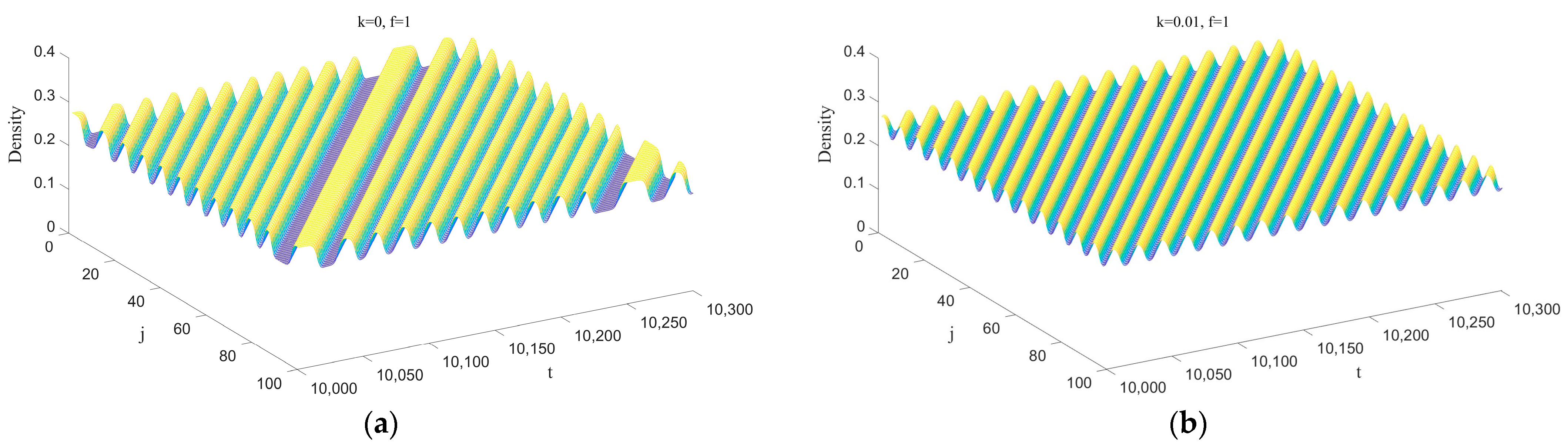
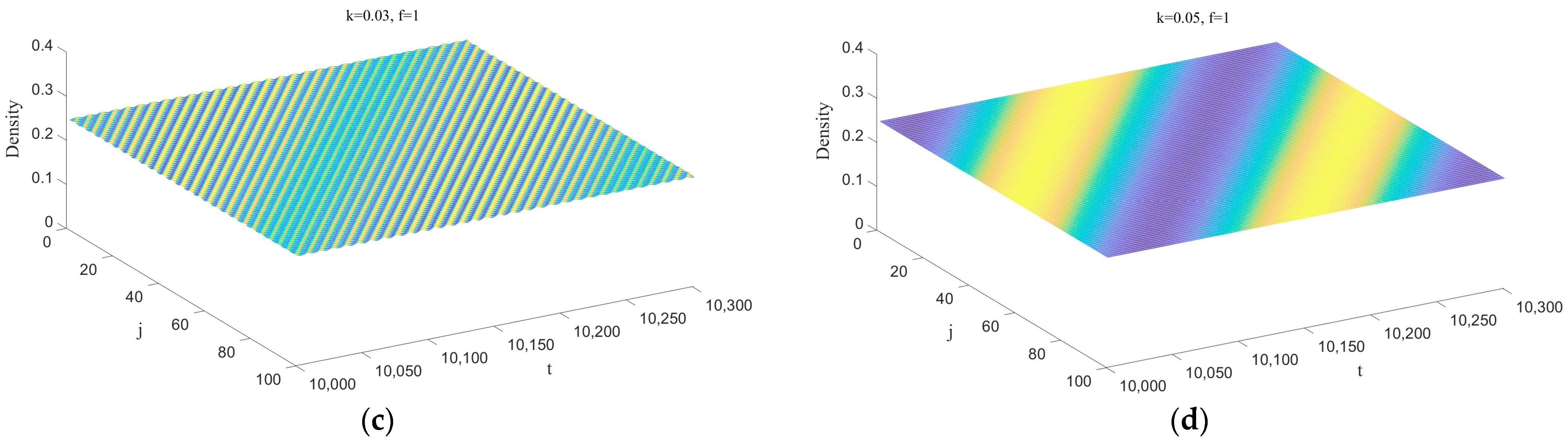
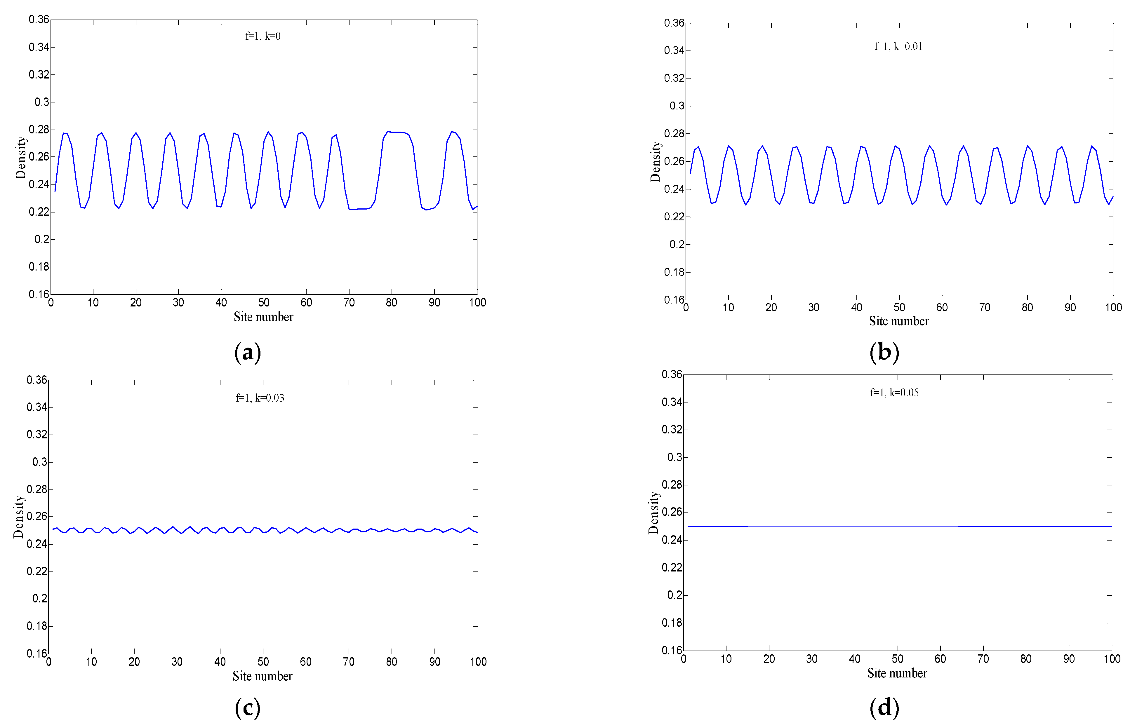
Figure 3 depicts the three-dimensional evolution of traffic density in the new model after 10,000 time steps, as the parameter k varies (taking values of 0, 0.01, 0.03, and 0.05). Here, the input parameter is set as f = 1. In Figure 3, subplots (a) to (d) correspond to the four different values of k. In subplot (a), when k = 0, the model degrades into the classic Nagatani two-lane lattice model. Since the desire effects of drivers’ smooth driving are not significantly considered at this point, disturbances gradually accumulate during propagation without being effectively suppressed, leading to the occurrence of stop-and-go traffic congestion. However, in subplots (b), (c), and (d), due to the notable incorporation of drivers’ desire for smooth driving, a remarkable contrast is observed compared to subplot (a), where traffic congestion is significantly alleviated, and traffic flow becomes smoother. Further observation reveals that as the parameter k gradually increases, the amplitude of traffic flow fluctuations gradually decreases. Especially when k = 0.05, corresponding to subplot (d), small disturbance signals are completely absorbed, and the traffic flow returns to its initial equilibrium state across the entire spatial range.

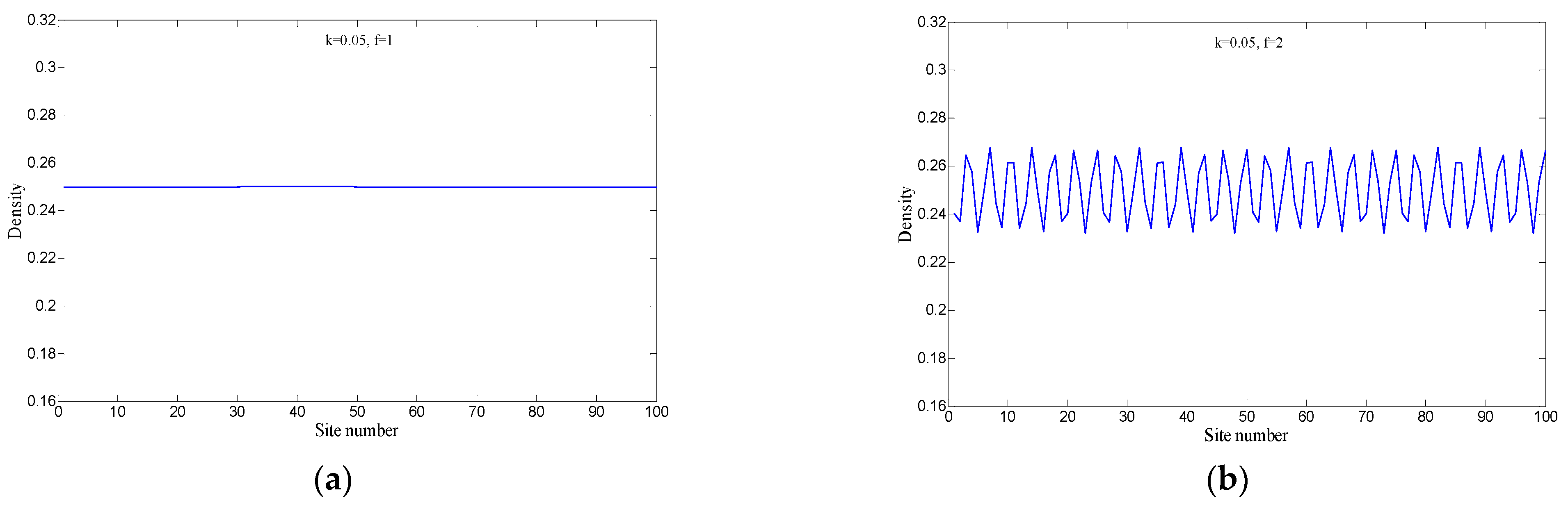
Corresponding to Figure 3 and Figure 4 depict the traffic density distribution across all lattice points in the new model at the 10,300 time step. From Figure 4, it is clearly visible that under the influence of small disturbances, the fluctuations of traffic flow amplify, forming kink-antikink density waves that lead to traffic congestion, with transitions occurring between the free-flow phase and the jammed phase. Meanwhile, as the parameter k increases, the fluctuation amplitude sharply decreases, gradually converging to the equilibrium state, and the frequency of transitions between the free-flow phase and the jammed phase also gradually decreases, resulting in smoother and more stable traffic flow. Especially in subplot (d), when the traffic density distribution reaches consistency across all lattice points, the traffic flow fully recovers to its initial steady state.

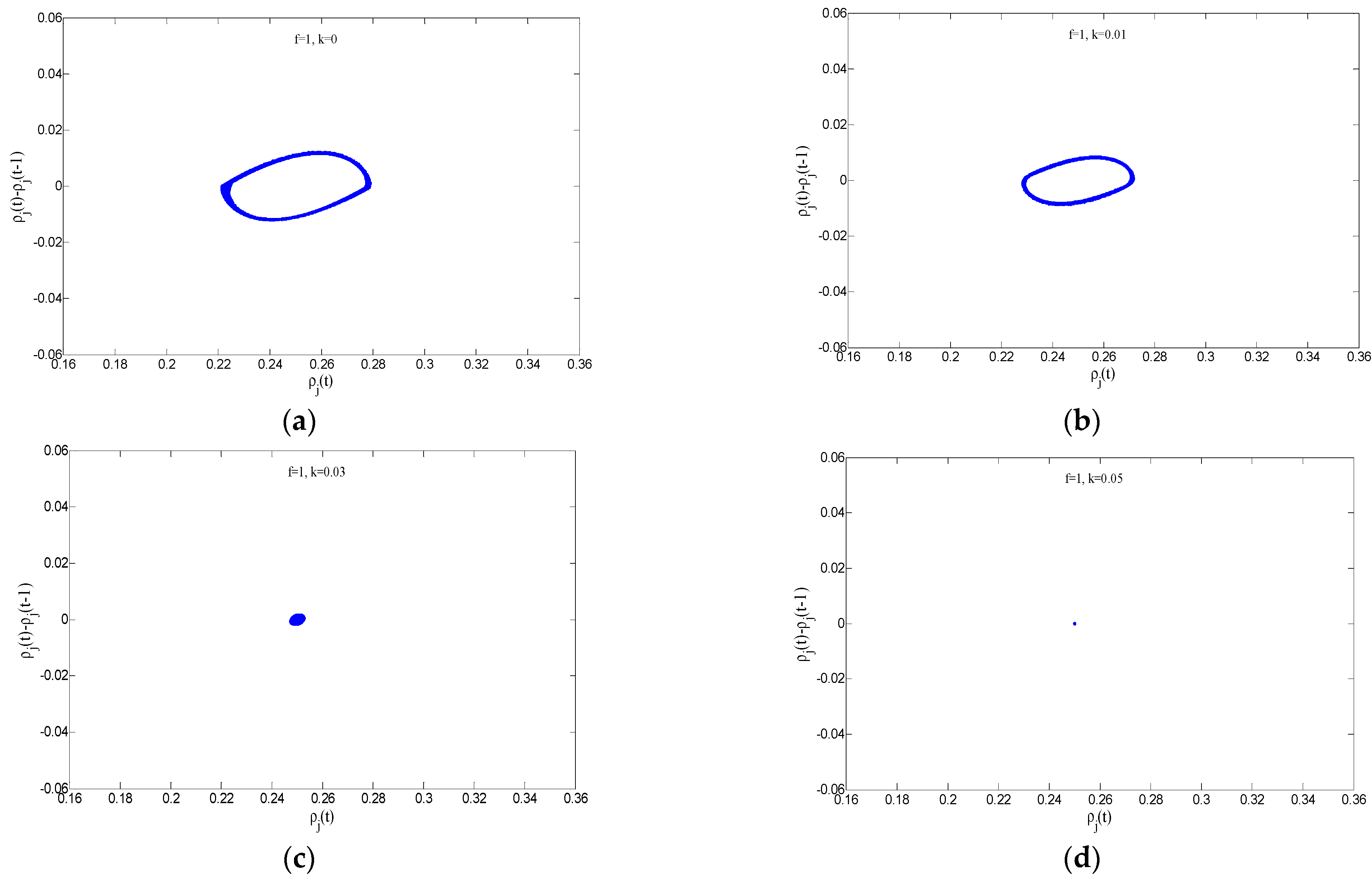
To more intuitively reveal the impact of the desire effects of drivers’ smooth driving on the stability of the transportation system in the two-lane system, Figure 5 plots the relationship between the density difference ${\rho }_j\left(t\right)-{\rho }_j\left(t-1\right)$ and the density ${\rho }_j\left(t\right)$ in the new model for different values of parameter k during a specific time period (from the 5000 to the 10,300 time step). The set of data points (${\rho }_j\left(t\right)-{\rho }_j\left(t-1\right)$) form a hysteresis loop. The area of the hysteresis loop intuitively reflects the stability of traffic operation: a smaller area indicates a more stable traffic operation. From Figure 5, it can be clearly observed that as the value of parameter k gradually increases, i.e., from subplots (a) to (d), the area of the hysteresis loop progressively decreases. Particularly noteworthy is that when the value of $k$ increases to 0.05, the hysteresis loop in Figure 5d almost degenerates into a single point, indicating that the density of all vehicles in the traffic flow is maintained at a stable state at this point.

In summary, the evolution processes of traffic flow in the two-lane system depicted in Figure 3, Figure 4 and Figure 5 consistently demonstrate that fully considering the desire effects of drivers’ smooth driving in actual traffic has a significant positive impact on the stability of traffic flow and can effectively suppress the formation of traffic congestion. This numerical simulation conclusion is fully consistent with the results of the linear stability theory analysis. Hence, the desire effects of drivers’ smooth driving are crucial for maintaining stable operation of traffic flow in two-lane systems.

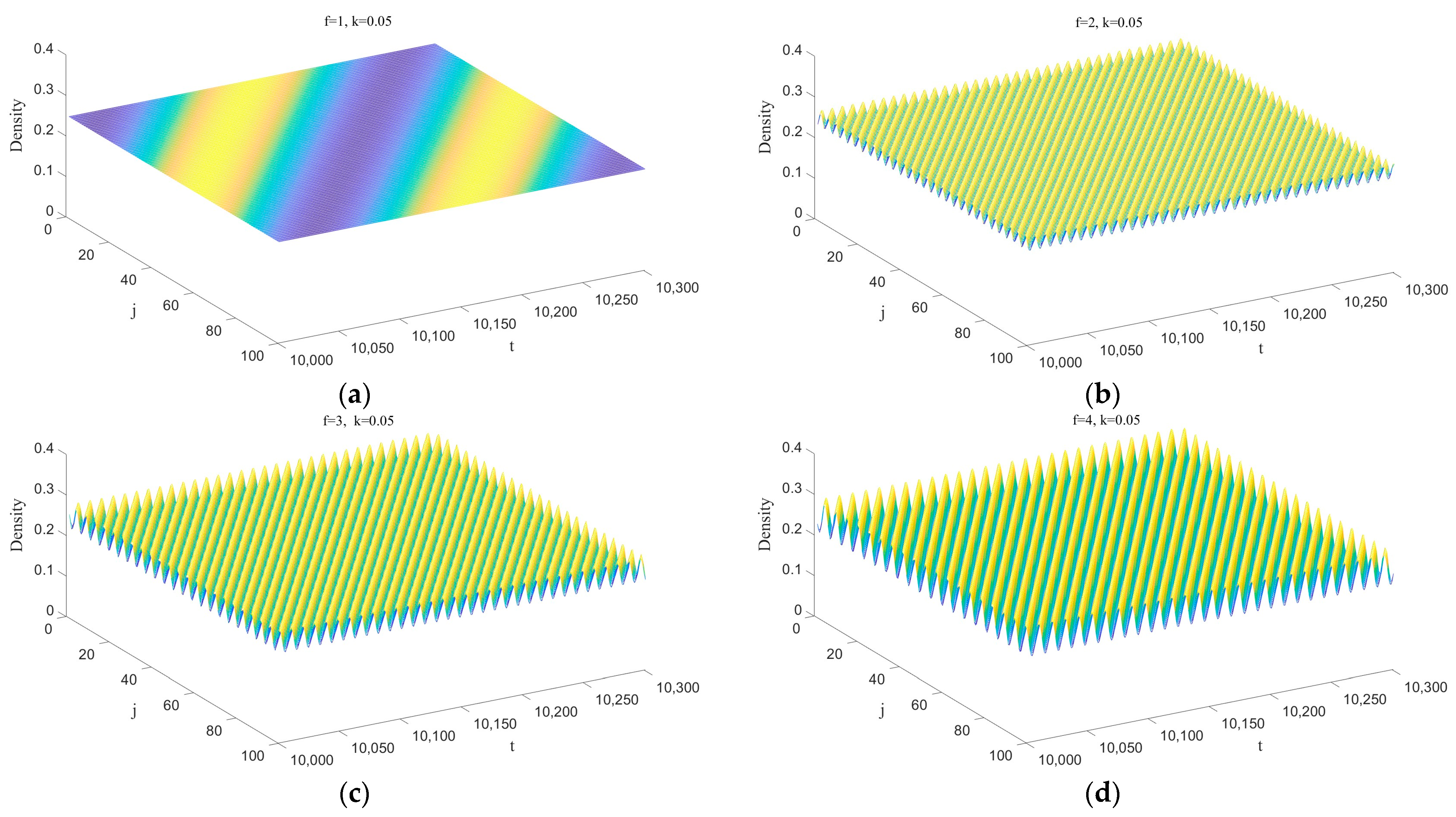
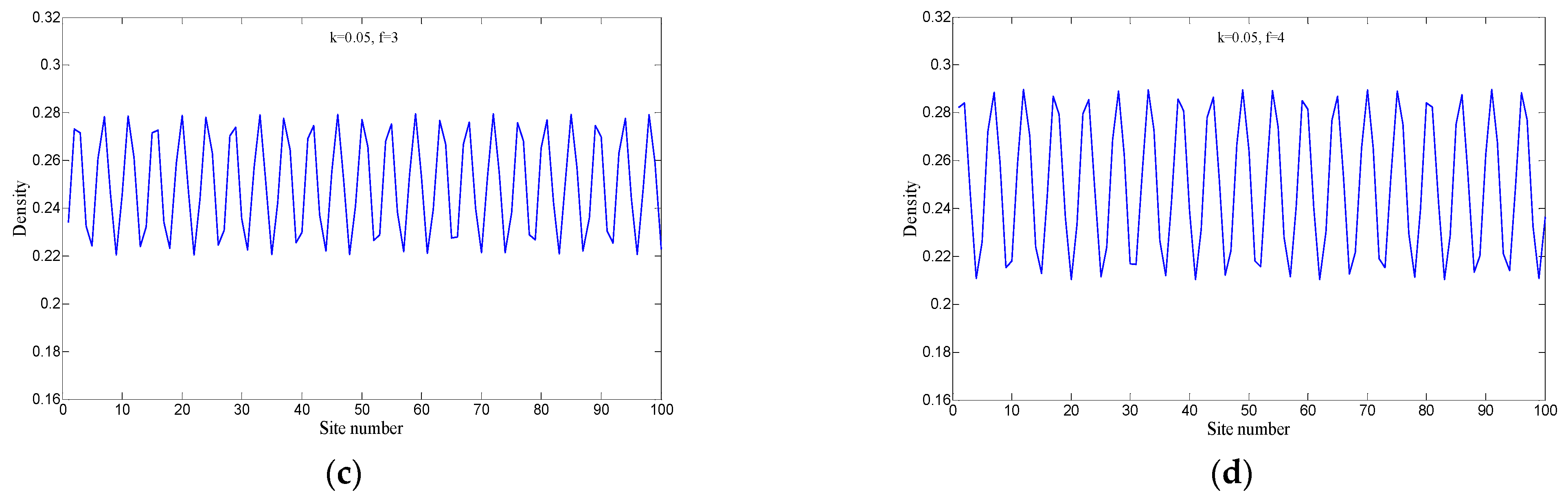
Figure 6 illustrates the three-dimensional evolution of traffic density corresponding to parameters f = 1, 2, 3, 4 after 10,000 time steps of evolution in the new model, with the input parameters set at k = 0.05. Corresponding to Figure 6 and Figure 7 display the traffic flow density distribution across all lattice points at the 10,300 time step. Through the traffic evolution processes depicted in Figure 6 and Figure 7, it is clearly observable that from subplot (d) to subplot (a), as parameter f decreases, the stability of the traffic flow in the two-lane system gradually improves. The alternation between sparse distributions of low-density traffic flow and clustered distributions of high-density traffic flow occurs less frequently, leading to smoother traffic operation. 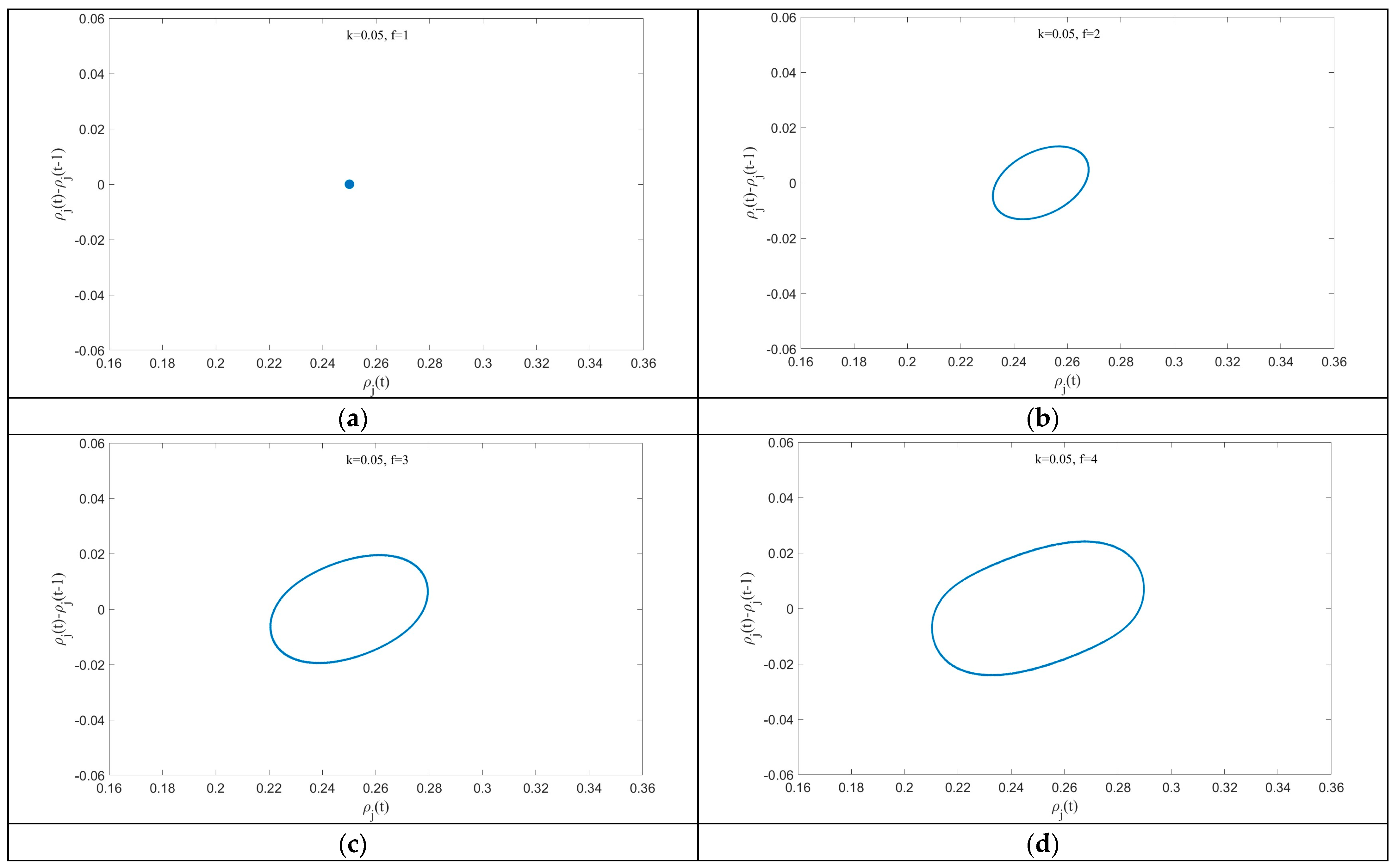Corresponding to Figure 6 and Figure 7, Figure 8 further presents the relationship between the density difference ${\rho }_j\left(t\right)-{\rho }_j\left(t-1\right)$ and the density ${\rho }_j\left(t\right)$ in the new model during the time period from t = 10,000 to 15,000. The figure reveals that as the value of parameter f decreases, from subplots (d) to (a), the area of the hysteresis loop becomes progressively smaller, with a smaller area indicating greater stability. Figure 6, Figure 7 and Figure 8 consistently demonstrate that the degree of driver lane-changing aggressiveness has a significant impact on the two-lane system, and as driver aggressiveness increases, the stability of the traffic flow is gradually enhanced. These simulation results are fully consistent with the findings of the linear stability theory analysis presented in Section 3.

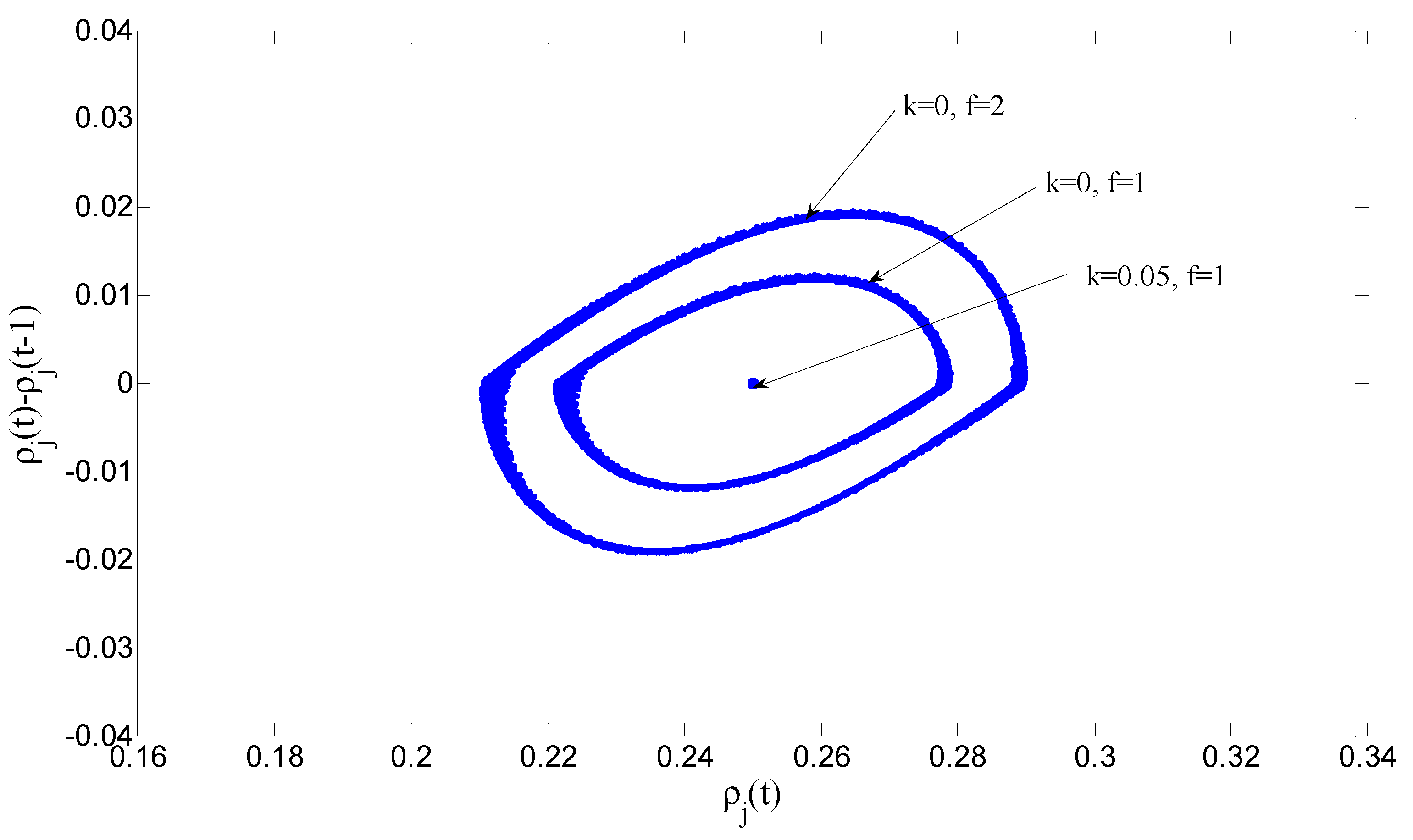
To further elucidate how the synergistic effect between drivers’ aggressive lane-changing behavior and their desire for smooth driving impacts traffic flow stability, Figure 9 shows the hysteresis loop phenomena generated by adjusting the parameters f (representing the aggressiveness of lane-changing behavior) and k (representing the intensity of the desire for smooth driving) to different levels in the new model. By closely comparing the curves under two specific parameter settings-specifically, when k = 0 and f = 1 versus k = 0 and f = 2—we observe that when k = 0, indicating that the model does not yet incorporate the driver’s desire for smooth driving, only the aggressive lane-changing behavior of drivers influences the stability of the two-lane system. Under these conditions, the area of the hysteresis loop decreases as the value of f decreases (i.e., as the lane-changing behavior becomes more aggressive), reflecting a certain degree of enhanced traffic flow stability. Nevertheless, it is noteworthy that the density difference ${\rho }_j\left(t\right)-{\rho }_j\left(t-1\right)$ does not consistently equal zero, signifying that variations in traffic density persist across consecutive time steps on the same road segment, and the system has not achieved complete stability. Furthermore, when we adjust the parameter k to 0.05, thereby introducing the driver’s desire for smooth driving, a notable shift occurs: the hysteresis loop phenomenon completely disappears, transforming into a single point. This transition indicates that the value of ${\rho }_j\left(t\right)-{\rho }_j\left(t-1\right)$ remains constantly zero, meaning that traffic density remains uniform at any two consecutive time points, marking a transition to a uniform and stable traffic flow state. This finding provides compelling evidence that when aggressive lane-changing behavior is combined with the driver’s desire for smooth driving, generating a synergistic effect, it can minimize fluctuations within traffic flow.

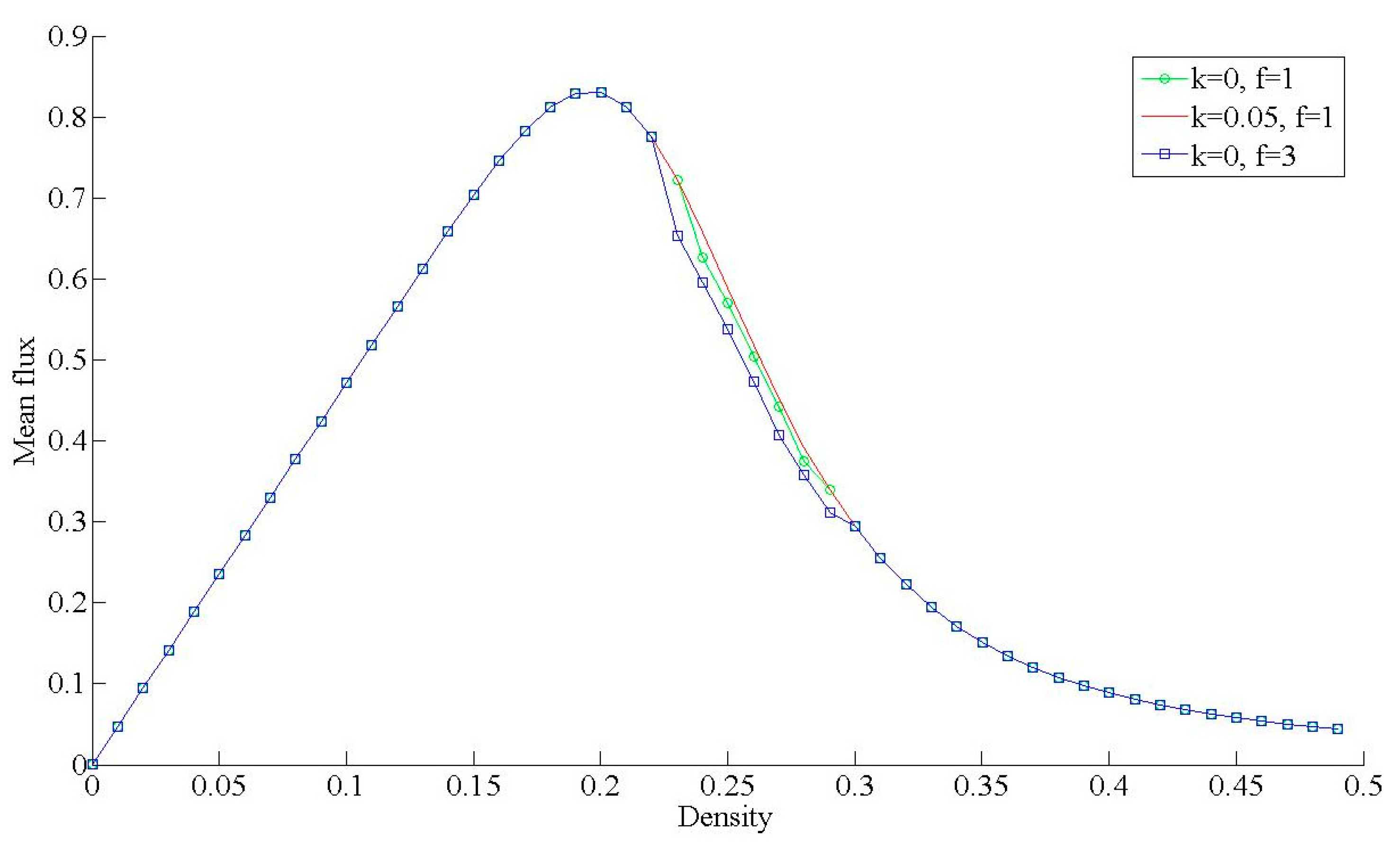
To investigate the synergistic effects of drivers’ smooth driving and aggressive lane-changing behaviors on traffic flux, we chose the 25th lattice site as the observation point. We collected flow data from this point during the time interval t = 10,000 – 10,300. Using these data, we performed statistical calculations to determine the mean flux value of the system. The total average density ${\rho }_0$ ranges from 0 to 0.5 in increments of 0.01. The initial conditions were set as follows:

$${\rho }_j\left(0\right)={\rho }_0, {\rho }_j\left(1\right)={\rho }_j\left(0\right)={\rho }_0, j\ne 50,51, {\rho }_j\left(1\right)={\rho }_0+0.1\mathrm{for}j=50{\rho }_j\left(1\right)=\max (0,{\rho }_0-0.1)\mathrm{for}j=51.$$

Figure 10 presents the simulation results.

Figure 10 shows the initial density versus mean traffic flow for different values of parameters $f$ and $k$ in the proposed model. Figure 10 indicates that in the low-density region (${\rho }_0<0.22$) and the high-density region (${\rho }_0>0.3$), the new factors considered in this paper have a relatively minor impact on the mean traffic flux of the two-lane system. However, in the intermediate-density region ($0.22\le {\rho }_0\le 0.3$), the influence of these new factors is more pronounced. When the parameters are set to k = 0 and f = 1, the proposed model corresponds to the classic Nagatani’s two-lane lattice model [2], in which the effect of drivers’ smooth driving is not taken into account, and only their aggressive lane-changing behavior is at play. It can be observed that in the intermediate-density region, the mean traffic flux under these conditions is higher than that when k = 0 and f = 3, suggesting that adopting a relatively aggressive lane-changing strategy can enhance the operational efficiency of the two-lane system to some extent. Furthermore, when we adjust the parameter $k$ to 0.05 (while keeping f = 1), the drivers’ aggressive lane-changing behavior and the smooth driving effect synergize, resulting in the maximum mean traffic flux of the two-lane system in the intermediate-density region. This finding fully demonstrates the importance and practical significance of the improvements made to the model in this paper.

In summary, the simulation results presented in Figure 4, Figure 5, Figure 6, Figure 7, Figure 8, Figure 9 and Figure 10 not only align closely with the linear stability theory analysis findings in Section 3, but the simulation experiments further confirm that, within a two-lane system, the synergistic strategy combining drivers’ aggressive lane-changing behaviors with their preference for smooth driving has a notable effect on enhancing traffic flow stability, optimizing overall traffic efficiency, and effectively alleviating traffic congestion. These significant findings provide valuable guidance for transportation management departments. Therefore, it is recommended to strengthen drivers’ maneuvering skills training and cognitive level enhancement, while also incorporating content on the synergistic strategy of aggressive lane-changing and smooth driving preferences into teaching materials and promotional efforts. This will ensure that drivers can apply these strategies in actual driving, thereby creating a more efficient traveling environment. Furthermore, when developing traffic simulation software, key factors such as drivers’ aggressive lane-changing behavior and their desire for smooth driving should be taken into account, in order to more accurately simulate and predict real-world road traffic flows, providing a more reliable basis for transportation planning and policy formulation.

6. Conclusions

In this paper, in order to address the deficiencies of the current two-lane lattice traffic flow model in considering driver behavior, we incorporate both drivers’ aggressive lane-changing behavior and their desire for smooth driving as co-acting factors into the model for the first time, proposing a novel two-lane lattice model. Through theoretical analysis, we not only derive the linear stability conditions of the new model but also obtain the density wave equation that describes the evolution of traffic congestion near the critical point, providing a theoretical foundation for the in-depth analysis of traffic flow dynamics. To verify the accuracy of the theoretical analysis, we conduct numerical simulation experiments under periodic boundary conditions, and the experimental results closely align with the theoretical analysis. The research findings indicate that in the two-lane system, increasing the drivers’ level of lane-changing aggressiveness alone or introducing the desired effect of smooth driving by drivers can both enhance traffic flow stability to a certain extent. However, when these two effects are considered in combination, i.e., exploring the synergistic effect of aggressive lane-changing behavior and the desire for smooth driving, we find that the stability of traffic flow is significantly improved, and the fluctuation amplitude of traffic congestion is further effectively suppressed. This discovery fully reveals the important influence of drivers’ aggressive lane-changing behavior and their desire for smooth driving on the stability of traffic flow in the two-lane system, as well as the positive impact of their synergistic effect. This provides new insights and directions for optimizing the management of two-lane traffic flow and mitigating traffic congestion.

However, the model developed in this paper only explores the dynamic characteristics of macroscopic traffic flow in two-lane scenarios. Recently, the modeling of macroscopic traffic flow in multi-lane systems (exceeding two lanes) has attracted the attention of scholars [38,39]. In our future work, we intend to extend the current model to multi-lane systems and take into consideration the impact of on- and off-ramps, in order to investigate the synergistic effect between drivers’ desires for smooth driving and their lane-changing behaviors in real-world traffic under more extensive conditions. Additionally, we also need to conduct calibration research on the model by measuring real-world traffic flow data, in order to further verify and refine our model.