Data-Driven Control Based on Information Concentration Estimator and Regularized Online Sequential Extreme Learning Machine

Abstract

Due to the complexity of digital equipment and systems, it is quite difficult to obtain a precise mechanism model in practice. For an unknown discrete-time nonlinear system, in this paper, a semi-parametric model is used to describe this discrete-time nonlinear system, and this semi-parametric model contains a parametric uncertainty part and a nonparametric uncertainty part. Based on this semi-parametric model, a novel data-driven control algorithm based on an information concentration estimator and regularized online sequential extreme learning machine (ReOS-ELM) is designed. The information concentration estimator estimates the parametric uncertainty part; The training data of ReOS-ELM network is obtained, based on symmetry and information concentration estimator, then the training of ReOS-ELM network and the estimate of nonparametric uncertainty part using ReOS-ELM network are carried out online, successively. A stability analysis and three simulation examples were performed, and the simulation results show that the proposed data-driven control algorithm is effective in improving the control accuracy.

1. Introduction

Data-driven control (DDC) algorithms rely on the input data and output data of control systems, and are very suitable for some nonlinear systems whose mechanism models cannot be established. After several years of development, some data-driven control techniques have been investigated, such as model free adaptive control (MFAC) [1,2,3,4,5], iterative learning control (ILC) [6,7,8,9], iterative feedback tuning (IFT) [10,11], unfalsified control (UC) [12,13], virtual reference feedback tuning (VRFT) [14], lazy learning control [15], some control algorithms based on neural networks [16,17,18,19], reinforcement learning [20,21,22,23,24], and so on. These DDC methods can be divided into two fundamental categories. The first one is that the controller structure is assumed to be known, then the controller design issue is transformed into a parametric synthesis, such as VRFT and IFT; the second one considers a system as an almost black-box model, it approaches the corresponding relationship between the input and output of systems as almost completely independent of the specific structure and parameters of systems, such as neural networks (NN) and MFAC.

For some nonlinear systems there is prior information about the control systems, these can be treated as linear systems to a certain extent, but this prior information is not enough for the first kind of DDC algorithm. NN do not consider prior information about control systems, but it is very difficult to explain their theory. In [25], a novel class of DDC algorithm was developed successfully for a simple first-order discrete-time nonlinear system. It is different from the previous two kinds of DDC algorithm, and divides a nonlinear system into a parametric uncertainty part and a nonparametric uncertainty part. The nonparametric uncertainty part was eliminated by the nearest-neighbor method. In [26], an extended version of an information concentration (IC) estimator was discussed for a second-order discrete-time nonlinear system. This IC estimator is effective when the parametric uncertainty part contains two unknown parameters. In [27], two independent IC estimators were adopted to estimate two unknown parameters of a speed control system of a robot arm. However, the nonparametric uncertainty part is assumed to be bounded, and this assumption is generally considered as a strict assumption. Furthermore, the stability of discrete-time nonlinear systems based on the extended version of the IC estimator was not guaranteed by theoretical analysis. In this paper, a data-driven control algorithm based on an IC estimator and regularized online sequential extreme learning machine (ReOS-ELM) is investigated for a discrete-time nonlinear system. Firstly, an improved IC estimator, which does not need the assumption that the nonparametric uncertainty part is bounded, is introduced. Secondly, a binary updating algorithm of ReOS-ELM is introduced, for stability analysis of the control system. Thirdly, the stability of the control system based on the proposed control algorithm is guaranteed by theoretical analysis. Finally, three simulation examples are performed. Compared with the existing results, there are two contributions. The first contribution is that this method does not need the assumption that the nonparametric uncertainty part is bounded. The second contribution is that the control system stability based on the proposed data-driven control algorithm based on the IC estimator is guaranteed by theoretical analysis.

This paper is structured as follows. The related knowledge is briefly introduced in Section 2. In Section 3, the proposed data-driven control algorithm based on an IC estimator and ReOS-ELM, including the parameter tuning for the data model as well as the stability issue, are stated. Simulation examples are stated in Section 4. Some conclusions are shown in Section 5.

2. Related Knowledge

2.1. Semi-Parametric Model

Modeling accurate mechanism models of actual systems is difficult due to their complex dynamic characteristics. Inspired by the research on the maximum capability and limitation of adaptive feedback mechanisms, some scholars designed a semi-parametric model. A semi-parametric model is different from a mechanism model; it is established depending on the historical data of a system and is used to describe discrete-time nonlinear systems. Semi-parametric models contain a parametric uncertainty part and a nonparametric uncertainty part. A semi-parametric model is described as

$$y_{k+1}={\mathsf{\varphi }}_k^T\mathsf{\theta }+u_k+g\left({\mathsf{\psi }}_k\right)+{\tau }_{k+1}$$

(1)

where $\mathsf{\theta }$ and $g(·)$:${\mathit{R}}^{d_2}\to \mathit{R}$ denote an unknown parameter vector and an unknown vector-valued function, respectively, and ${\tau }_k$ denotes random noise. Here, ${\mathsf{\varphi }}_k^T\mathsf{\theta }$ and $u_k+g\left({\mathsf{\psi }}_k\right)$ are considered as parametric uncertainty part and nonparametric uncertainty part, respectively. From Equation (1), it is derived that $y_{k+1}-{\mathsf{\varphi }}_k^T\mathsf{\theta }-{\tau }_{k+1}$ and nonparametric uncertainty part are symmetrical.

The regression vectors ${\mathsf{\varphi }}_k$ and ${\mathsf{\psi }}_k$, are composed of historical data,

$${\mathsf{\varphi }}_k={\left[y_k,y_{k-1},\cdots ,y_{k-p_1+1},u_{k-1},\cdots ,u_{k-q_1}\right]}^T$$

(2)

and

$${\mathsf{\psi }}_k=\left[y_k,y_{k-1},\cdots ,y_{k-p_2+1},u_{k-1},\cdots ,u_{k-q_2}\right]$$

(3)

Here, $d_1$ and $d_2$ are the dimensions of the regression vectors ${\mathsf{\varphi }}_k$ and ${\mathsf{\psi }}_k$,

$$d_1=q_1+p_1$$

(4)

and

$$d_2=q_2+p_2$$

(5)

2.2. Information Concentration Estimator

The classic self tuning regulator based on least squares (LS) can be applied to autoregressive exogenous systems, while the recursive least-squares algorithm can estimate unknown parameters of linear systems. The performance of traditional real-valued parameter identification on nonlinear systems which contain large nonparametric uncertainty is not very outstanding. Different from traditional real-valued parameter identification methods, the IC estimator regards prior knowledge at each step as some constraint on unknown parameters or functions, and reduces parameter or function uncertainties based on the prior knowledge step by step by using geometry knowledge. Its basic idea, which is depicted in Figure 1, is to test each vertex of $v_k$ to see whether to keep the original vertex or to generate a new vertex. At time k, the center point of the polygon domain $I_k$ is generally taken as ${\widehat{\mathsf{\theta }}}_k$. When the straight line intersects the polygon v, and splits it into two sub-polygons, the $n_k$ of the new polygon $v{}^{\prime }$ may become large or small. Figure 1b shows that $n_k$ will become large.

2.3. Regularized Online Sequential Extreme Learning Machine

The online sequential extreme learning machine (OS-ELM) [28] is an online learning algorithm, and it often is used to train single-hidden-layer feed forward neural (SLFN) networks online. ReOS-ELM [29] is an improved version of OS-ELM, and it adds a regular term to the cost function.

For a single-hidden-layer neural network which is composed of n input nodes, L hidden nodes, and one output node, the jth output corresponding to the jth input pattern can be represented by

$$o_j=\sum _{i=1}^L{\beta }_{i}G({\mathit{w}}_i,b_i,{\mathit{x}}_j),j=1,\cdots ,N_0$$

(6)

where ${\mathit{x}}_j$ and $o_j$ denote the jth input pattern and the jth output, respectively; $b_i$ is a bias of the active function $G(·)$; and ${\mathit{w}}_i$ and ${\beta }_i$ are two weights which are used to connect the input node and the ith hidden node, and the ith hidden node and the output node, respectively.

For an initial training dataset with $N_0$ training patterns $({\mathit{x}}_j,t_j)\in {\mathit{R}}^n\times \mathit{R}$, where ${\mathit{x}}_j={[x_{j1},x_{j1},\cdots ,x_{jn}]}^T$, OS-ELM adopts Equation (7) as the cost function for the goal of determining the output weights in the training process.

$$\parallel {\mathit{H}}_0{\mathit{\beta }}_0-{\mathit{T}}_0{\parallel }^2$$

(7)

The cost function (7) is sensitive to noise, and noise would lead to a poor generalization and over-fitting. In order to reduce the influence caused by noise, ReOS-ELM [30], which adds a regularization factor $\lambda$ to the cost function for the purpose of controlling the trade-off between the output weight norm and the training error, is proposed based on Tikhonov regularization. The improved cost function is

$$\parallel {\mathit{H}}_0{\mathit{\beta }}_0-{\mathit{T}}_0{\parallel }^2+\lambda {\parallel {\mathit{\beta }}_0\parallel }^2$$

(8)

where

$${\mathit{T}}_0={\left[t_1,\cdots ,t_{N_0}\right]}^T$$

(9)

and

$${\mathit{H}}_0={\left[\begin{array}{ccc}G({\mathit{w}}_1,b_1,{\mathit{x}}_1)& \cdots & G({\mathit{w}}_L,b_L,{\mathit{x}}_1)\\ ⋮& \cdots & ⋮\\ G({\mathit{w}}_1,b_1,{\mathit{x}}_{N_0})& \cdots & G({\mathit{w}}_L,b_L,{\mathit{x}}_{N_0})\end{array}\right]}_{N_0\times L}$$

(10)

The solution of ${\mathit{\beta }}_0$ is

$${\mathit{\beta }}_0={\mathit{P}}_0{\mathit{H}}_0^T{\mathit{T}}_0$$

(11)

where

$${\mathit{P}}_0={({\mathit{H}}_0^T{\mathit{H}}_0+\lambda {\mathit{I}}_L)}^{-1}$$

(12)

and ${\mathit{I}}_L$ is an identity matrix of size L (number of hidden nodes).

When the kth chunk of the dataset is received

$$N_k=\left\{({\mathit{x}}_i,t_i)\right\}{}_{i={\sum }_{j=0}^{k-1}{N}_j+1}^{i={\sum }_{j=0}^k{N}_j}$$

(13)

ReOS-ELM takes a similar form to recursive least squares (RLS) to update the weight connecting the hidden node and output node, and the weight updating algorithm is as follows:

$${\mathit{P}}_k={\mathit{P}}_{k-1}-\frac{{\mathit{P}}_{k-1}{\mathit{H}}_k^T{\mathit{H}}_k{\mathit{P}}_{k-1}}{{\mathit{I}}_{N_k}+{\mathit{H}}_k{\mathit{P}}_{k-1}{\mathit{H}}_k^T}$$

(14)

and

$${\mathit{\beta }}_k={\mathit{\beta }}_{k-1}+{\mathit{P}}_k{\mathit{H}}_k^T({\mathit{T}}_k-{\mathit{H}}_k{\mathit{\beta }}_{k-1})$$

(15)

where ${\mathit{T}}_k$ and ${\mathit{H}}_k$ indicate the target of the kth arriving training data and the hidden layer output for the kth arriving training data, respectively, and ${\mathit{I}}_{N_k}$ is an identity matrix of size $N_k$.

2.4. Problem Formulation

In this paper, the following second-order nonlinear system is considered:

$$y_{k+1}={\vartheta }_1{y}_k+{\vartheta }_2{y}_{k-1}+u_k+f(y_k,y_{k-1})$$

(16)

where $y_k$ and $u_k$ are the output signal and input signal of the system (16), respectively. ${\vartheta }_1$ and ${\vartheta }_2$ are two unknown parameters, $f(·)$ is an unknown nonlinear function, and $f(·)\in F\left(L\right)$, which indicates the nonparametric uncertainty part of the system (16). Here, $F\left(L\right)$ (the set $F\left(L\right)$ will be defined later) represents a priori knowledge on possible $f(·)$.

In this paper, the following assumptions need to be guaranteed for making further study.

Assumption 1. 

The reference signal $\left\{y_k^{*}\right\}$ is bounded, i.e.,

$$\left|y_k^{*}\right|⩽B_{\omega },\forall k⩾0$$

(17)

where $B_{\omega }$ is a positive constant.

Assumption 2. 

Each element of the unknown vector $\mathsf{\theta }$ is bounded by two known constants ${\overline{B}}_{\theta ,j}$ and ${\underline{B}}_{\theta ,j}$, i.e., for $j=1,2$

$${\underline{B}}_{\theta ,j}⩽{\vartheta }_j⩽{\overline{B}}_{\theta ,j}$$

(18)

Assumption 3. 

The unknown function f belongs to the following uncertainty set

$$F\left(L\right)=\{f:|f(x_1,y_1)-f(x_0,y_0)|\le L_M\parallel (x_1,y_1)-(x_0,y_0)\parallel +L_c\}$$

(19)

where $L_M<\frac{3}{2}+\sqrt{2}$.

3. The Design of Data-Driven Control Using the Proposed IC Estimator and ReOS-ELM

In [26], the nonparametric uncertainty part was supposed to be bounded. As time passes, $n_k$ may become very large, and so it takes a lot of time to calculate ${\widehat{\mathsf{\theta }}}_k$. In this paper, an improved IC estimator is introduced and used to estimate the unknown parameters of the parametric uncertainty part. The improved IC estimator adopts a constraint form which is from the constraint form in [26], but it consists of two steps of history data, which is different from the previous result, and the previous result needs step history data as well as the assumption that the nonparametric uncertainty part of the actual system is bounded. The improved IC estimator only needs to meet with Assumption 3. In addition, the problem that $n_k$ may be very large is considered, the number of vertexes is restricted to 10, and if $n_k>10$, the case of Figure 1b is ignored. Equation (16) can be rewritten as

$$y_{k+1}={\widehat{\vartheta }}_{1,k}{y}_k+{\widehat{\vartheta }}_{2,k}{y}_{k-1}+u_k+f_1(y_k,y_{k-1})$$

(20)

where

$$f_1(y_k,y_{k-1})={\tilde{\vartheta }}_{1,k}{y}_k+{\tilde{\vartheta }}_{2,k}{y}_{k-1}+f(y_k,y_{k-1})$$

(21)

and ${\tilde{\vartheta }}_{1,k}={\vartheta }_1-{\widehat{\vartheta }}_{1,k}$, ${\tilde{\vartheta }}_{2,k}={\vartheta }_2-{\widehat{\vartheta }}_{2,k}$, and ${\widehat{\vartheta }}_{1,k}$ and ${\widehat{\vartheta }}_{2,k}$ are the estimated values of ${\vartheta }_1$ and ${\vartheta }_2$ by the IC estimator at time k. As time passes and more data is accumulated, more and more constraints on the true parameters ${\vartheta }_1$ and ${\vartheta }_2$ can be obtained, and the parameter or function uncertainties become smaller, and finally the values ${\widehat{\vartheta }}_{1,k}$ and ${\widehat{\vartheta }}_{2,k}$ become fixed values.

Assumption 4. 

For $f_1(y_k,y_{k-1})$, suppose that there is ${\mathit{\beta }}^{*}$, then $f_1(y_k,y_{k-1})$ can be rewritten as

$$f_1(y_k,y_{k-1})={\mathit{H}}_k{\mathit{\beta }}^{*}+{▵}_k$$

(22)

where

$${\mathit{H}}_k{\mathit{\beta }}^{*}=\sum _{i=1}^L{\beta }_i^{*}G({\mathit{w}}_i,b_i,{\mathit{x}}_k)$$

(23)

$${\mathit{x}}_k=\left[y_k,y_{k-1}\right]$$

(24)

and $sup|{▵}_k|\le ▵$, $▵$ is a given upper bound, and ${\mathit{w}}_i$, $b_i$ can be randomly generated and kept constant.

In this paper, the unknown parameters ${\vartheta }_1$ and ${\vartheta }_2$ are estimated by the IC estimator, and the unknown nonlinear term $f_1(y_k,y_{k-1})$ is approached by a single-hidden-layer NN. The controller is developed by

$$u_k=u_k^l-u_k^c$$

(25)

where $u_k^l$ indicates the output of a controller which is used to stabilize linearized dynamics,

$$u_k^l=y_{k+1}^{*}-{\widehat{\vartheta }}_{1,k}{y}_k-{\widehat{\vartheta }}_{2,k}{y}_{k-1},$$

(26)

and here $u_k^c$ is the output of a single-hidden-layer NN.

$$u_k^c={\mathit{H}}_k{\widehat{\mathit{\beta }}}_k$$

(27)

where ${\widehat{\mathit{\beta }}}_k$ is the estimated value of the ideal weight vector ${\mathit{\beta }}^{*}$. The detailed design for the proposed improved IC estimator is shown in Section 3.1. The updating algorithm for the ideal weight vector connecting hidden nodes and output nodes adopts a binary form, and the detailed content of the binary form is introduced in Section 3.2.

3.1. The Design for the Proposed Improved IC Estimator

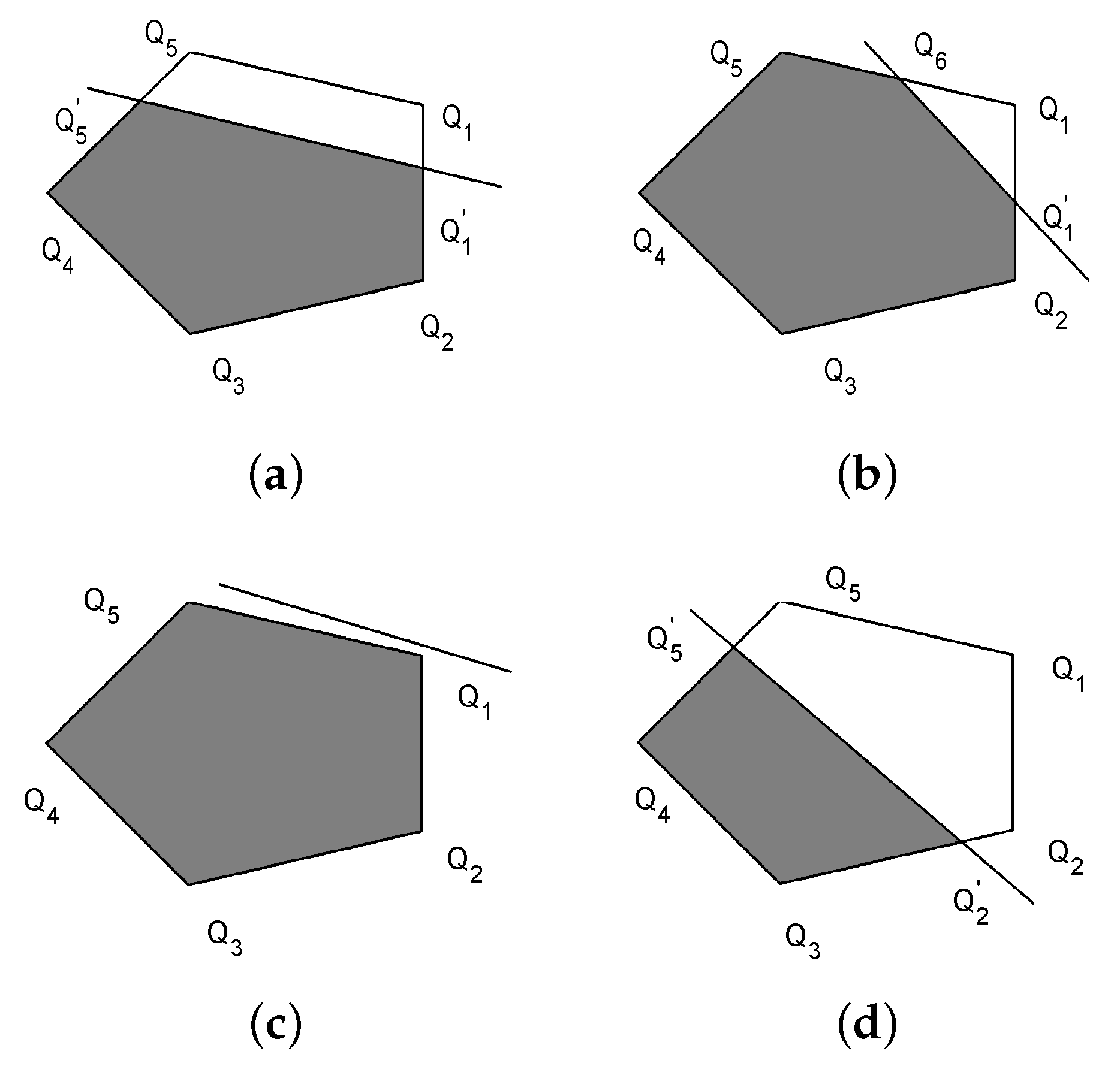
Define

$$J_k\triangleq y_k-u_{k-1}$$

(28)

For the discrete-time nonlinear system (16) with a priori knowledge $\mathsf{\theta }\in \Theta \subseteq {\mathit{R}}^2$, at the kth step ($k⩾0$), with the data $y_k$ coming, the so-called information set $I_k$ is defined as

$$I_k\triangleq \mathsf{\theta }\in \Theta :J_k-J_{k-1}-({\mathsf{\varphi }}_{k-1}^T-{\mathsf{\varphi }}_{k-2}^T)\mathsf{\theta }\in F$$

(29)

where the initial set $I_0=\Theta$.

Combined with Assumption 2, Assumption 3, and (29), we have the following form of parametric uncertainty at time k

$$\begin{array}{c}\hfill J_k-J_{k-1}-L_M\parallel (y_{k-1},y_{k-2})-(y_{k-2},y_{k-3})\parallel -L_c⩽({\mathsf{\varphi }}_{k-1}^T-{\mathsf{\varphi }}_{k-2}^T)\mathsf{\theta }\\ \hfill ({\mathsf{\varphi }}_{k-1}^T-{\mathsf{\varphi }}_{k-2}^T)\mathsf{\theta }⩽J_k-J_{k-1}+L_M\parallel (y_{k-1},y_{k-2})-(y_{k-2},y_{k-3})\parallel +L_c\end{array}$$

(30)

Hence, we can obtain the specific constraint form $I_k$ about parameter vector $\mathsf{\theta }$, and it consists of two independent inequalities:

$$({\mathsf{\varphi }}_{k-1}^T-{\mathsf{\varphi }}_{k-2}^T)\mathsf{\theta }⩽c_{k,1},-({\mathsf{\varphi }}_{k-1}^T-{\mathsf{\varphi }}_{k-2}^T)\mathsf{\theta }⩽c_{k,2}$$

(31)

where

$$\begin{array}{cc}\hfill c_{k,1}& =J_k-J_{k-1}+L_M\parallel (y_{k-1},y_{k-2})-(y_{k-2},y_{k-3})\parallel +L_c\hfill \\ \hfill c_{k,2}& =-(J_k-J_{k-1}-L_M\parallel (y_{k-1},y_{k-2})-(y_{k-2},y_{k-3})\parallel -L_c)\hfill \end{array}$$

(32)

Then, the so-called concentrated information set $C_k$ at step k is

$$C_k=\bigcap _{j=0}^k{I}_k=C_{k-1}\bigcap I_k$$

(33)

where $C_0=I_0$.

Generally, $C_k$ is a domain in ${\mathit{R}}^2$, and the area of $C_k$ would shrink over time. The actual parameter vector $\mathsf{\theta }$ may be located at anywhere in $C_k$, and in the simulation experiment, the center point of $C_k$ is adopted as an estimated value of the parameter vector $\mathsf{\theta }$ at the kth step.

The key problem of the IC estimator is to calculate the information set $I_k$ and the concentrated information set $C_k$ at each step. According to the basic idea of information concentration, these two constraints (32) are added one by one. i.e.,

$$\begin{array}{cc}\hfill v_{k-1}{}^{\prime }& =\mathrm{AddLinearCons}2\mathrm{D}(v_{k-1},({\mathsf{\varphi }}_{k-1}^T-{\mathsf{\varphi }}_{k-2}^T),c_{k,1}),\hfill \\ \hfill v_k& =\mathrm{AddLinearCons}2\mathrm{D}(v_{k-1}{}^{\prime },-({\mathsf{\varphi }}_{k-1}^T-{\mathsf{\varphi }}_{k-2}^T),c_{k,2})\hfill \end{array}$$

(34)

where $v_k=\{Q_i,i=1,2,\cdots ,n_k\}$ denotes the different vertexes of the domain $C_k$, and $n_k$ denotes the number of vertexes. $\mathrm{AddLinearCons}2\mathrm{D}$ is the core of the IC estimator. The pseudo code of $\mathrm{AddLinearCons}2\mathrm{D}$ is shown in Algorithm 1.

Algorithm 1: AddLinearCons2D($v,\mathsf{\varphi },c$): Add linear constraint ${\mathsf{\varphi }}^T\mathsf{\theta }\le c(\mathsf{\varphi }\in {\mathit{R}}^2)$ to a polygon v.

Input: $v:$ represented by clock-wise arranged vertexes $Q_1,Q_2,\cdots ,Q_n$

Output: $v{}^{\prime }:$ clock-wise arranged vertexes

1: Denote the number of vertexes in v by n

2: for $j=1$ to n do

3:    Denote the jth vertex by $Q_j$

4:    Let $F_i=\mathrm{sign}(c-\mathsf{\varphi }{Q}_j)$.

5: end for

6: if $F_j\ge 0,\forall 1⩽j⩽n$ then

7:    $v{}^{\prime }\leftarrow v$ and return

8: else if $F_j<0$,$\forall 1⩽j⩽n$ then

9:    $v{}^{\prime }\leftarrow \varnothing$ and return

10: end if

11: for $j=2$ to $n-1$ do

12:    if ($Q_j$ and $Q_{j-1}$ are in different side) ∧ ($Q_j$ and $Q_{j+1}$ are in different sides) then

14:       $Q_1^i\leftarrow$ the intersection of $l_i$ and $\overline{Q_{j-1}{Q}_j}$

15:       $Q_2^i\leftarrow$ the intersection of $l_i$ and $\overline{Q_{j+1}{Q}_j}$

16:          if ($F_j>0$) then

17:             $v{}^{\prime }=\{Q_1^i,Q_j,Q_2^i\}$

18:          else

19:             $v{}^{\prime }=\{Q1,\cdots ,Q_{j-1},Q_1^i,Q_2^i,Q_{j+1},·,Q_n\}$

20:          end if

21:       break

22:       else if ($Qj$ and $Q_{j-1}$ are in different side) ∧ ($Q_j,Q_{j+1},\cdots ,$ $Q_{j+a-1}$ are on

the same side) ∧ ($Q_{j+a-1},Q_{j+a}$ are on different side) then

23:          $Q_1^i\leftarrow$ the intersection of $l_i$ and $\overline{Q_{j-1}{Q}_j}$

24:          $Q_2^i\leftarrow$ the intersection of $l_i$ and $\overline{Q_{j+a-1}{Q}_{j+a}}$

25:             if $F_j>0$ then

26:                $v{}^{\prime }$={$Q_1^i,Q_j,\cdots ,Q_{j+a-1},Q_2^i$}

27:             else

28:                $v{}^{\prime }$=$\{Q_1,\cdots ,Q_{j-1},Q_1^i,Q_2^i{Q}_{j+a},\cdots ,Q_n\}$

29:             end if

30:       break

31:          else if ($Q_j$ and $Q_{j-1}$ are in different side) ∧ ($Q_{j-1}{Q}_{j-2},\cdots ,Q_1$ are on the,

same side) ∧ ($Q_j,\cdots ,Q_n$ are the same side) then

32:             $Q_1^i\leftarrow$ the intersection of $l_i$ and $\overline{Q_1{Q}_n}$

33:             $Q_2^i\leftarrow$ the intersection of $l_i$ and $\overline{Q_{j-1}{Q}_j}$

34:                   if $F_j>0$ then

35:                      $v{}^{\prime }$={$Q_1^i,Q_j,\cdots ,Q_n,P_2^i$}

36:                   else

37:                      $v{}^{\prime }$={$Q_2^i,Q_1,\cdots ,Q_{j-1},Q_1^i$ }

38:                   end if

39:          break

40:          end if

41:       end if

42:    end if

43: $j\leftarrow j+1$

44: end for

46: if (size$\left(v{}^{\prime }\right)>$10) then

47:    $v{}^{\prime }=v$

48: else

49:    $v{}^{\prime }=v{}^{\prime }$

50: end if

51: return $v{}^{\prime }$

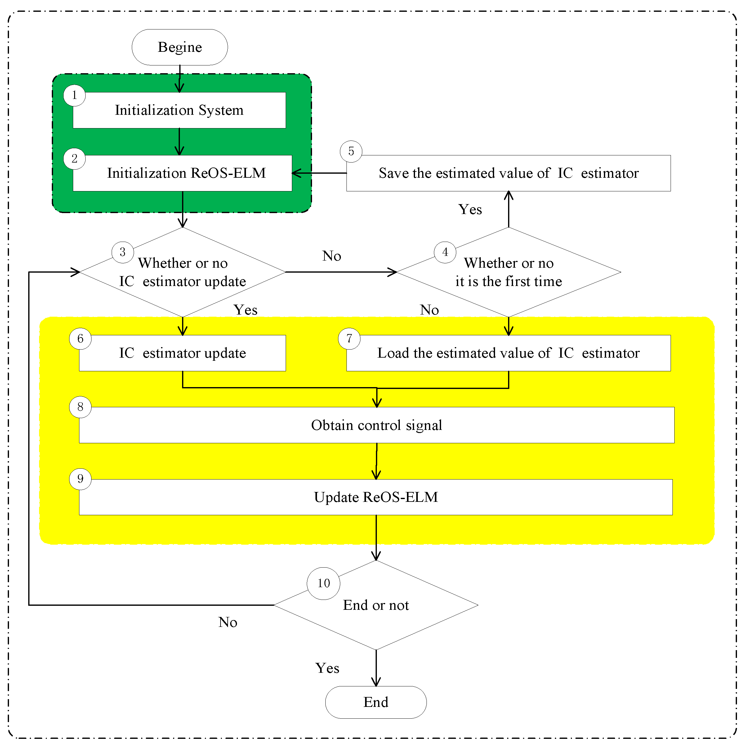
3.2. The Design of the Data-Driven Control Algorithm

The proposed data-driven control algorithm based on the IC estimator and ReOS-ELM network is performed in two main stages: the first stage is system initialization and the second stage is parameter learning. The process of the proposed data-driven control algorithm is shown in Figure 2.

➀

Initialization of System

• According to a priori knowledge on $\mathsf{\theta }$, we can obtain the initial polygon $V_1$ (usually a quadrangle) and the value of ${\widehat{\mathsf{\theta }}}_1$, and define $V_3\triangleq V_2\triangleq V_1$, ${\widehat{\mathsf{\theta }}}_3\triangleq {\widehat{\mathsf{\theta }}}_2\triangleq {\widehat{\mathsf{\theta }}}_1$, set $k_m=50$.
• Set $y_1=0$, and $y_2=u_1$; $u_1$, $u_2$ are two random numbers, $|u_1|\le 0.5$, and $|u_2|\le 0.5$; set $\epsilon =0.06$, ${\delta }_1=0.4$, ${\delta }_2=0.05$, and $k=3$.

➁

Initialization of ReOS-ELM

• For ReOS-ELM, define the hidden node number L, and the regularization factor $\lambda$.
• Assign random parameters $({\mathit{w}}_i,b_i)$ for ReOS-ELM, where $i=1,2,\cdots ,L$.
• Measure the output $y_3$ of the plant (16).
• The first sampling data can be obtained as ${\mathit{x}}_1=(y_2,y_1)$ and $t_1=e_3=y_3-{\widehat{\vartheta }}_{1,1}{y}_2-{\widehat{\vartheta }}_{1,2}{y}_1-u_2$.
• Obtain ${\mathit{P}}_1$ and $\widehat{{\mathit{\beta }}_1}$ using the following equations

  $${\mathit{P}}_1={(\lambda {\mathit{I}}_L+{\mathit{H}}_1^T{\mathit{H}}_1)}^{-1}$$

  (35)

  and

  $${\widehat{\mathit{\beta }}}_1={\mathit{P}}_1{\mathit{H}}_1^T{e}_3$$

  (36)
  Define ${\widehat{\mathit{\beta }}}_3\triangleq {\widehat{\mathit{\beta }}}_2\triangleq {\widehat{\mathit{\beta }}}_1$, and ${\mathit{P}}_3\triangleq {\mathit{P}}_2\triangleq {\mathit{P}}_1\triangleq {\mathit{P}}_0$.
• Set $Flag=0$, which means that the relearning process has not been activated.

➂

Whether or not the IC estimator updates

• Calculate ${\mathit{\sigma }}_k$ and

  $${\mathit{\sigma }}_k=[{\sigma }_{n_k}\left(1\right),{\sigma }_{n_k}\left(2\right)]$$

  (37)

  where

  $$\begin{array}{cc}\hfill {\sigma }_{n_k}\left(1\right)& =\mathrm{var}(X_{Q_1},X_{Q_2},\cdots ,X_{Q_{n_k}})\hfill \\ \hfill {\sigma }_{n_k}\left(2\right)& =\mathrm{var}(Y_{Q_1},Y_{Q_2},\cdots ,Y_{Q_{n_k}})\hfill \end{array}$$

  (38)

  and $X_Q$ and $Y_Q$ denote the two coordinates of Q.
• if ${\sigma }_{n_k}\left(1\right)>{\delta }_1\wedge {\sigma }_{n_k}\left(2\right)>{\delta }_1$, then execute ➅ or ➃.

➃

Whether or not it is the first time

• Calculate ${\xi }_k\left(1\right)$ and ${\xi }_k\left(2\right)$. If $k<11$, execute

  $$\begin{array}{cc}\hfill {\xi }_k\left(1\right)& =\mathrm{var}({\widehat{\theta }}_{1,k-10},\cdots ,{\widehat{\theta }}_{1,k})\hfill \\ \hfill {\xi }_k\left(2\right)& =\mathrm{var}({\widehat{\theta }}_{2,k-10},\cdots ,{\widehat{\theta }}_{2,k})\hfill \end{array}$$

  (39)

  or ${\xi }_k\left(1\right)=1,{\xi }_k\left(2\right)=1$.
• If $({\sigma }_{n_k}\left(1\right)<{\delta }_2\wedge {\sigma }_{n_k}\left(2\right)<{\delta }_2)\vee ({\xi }_k\left(1\right)\le \epsilon \wedge {\xi }_k\left(2\right)\le \epsilon \wedge k\ge k_m\wedge Flag=0)$, then set $Flag=1$.
• if $Flag=0$, execute ➄ or ➆.

➄

Initialize ReOS-ELM and save the estimated value of the IC estimator

• Relearning: using the data ${\mathit{x}}_k=\left[y_k,y_{k-1}\right]$ and $e_{k+1}$ initialize ReOS-ELM, and obtain ${\mathit{P}}_k$ and ${\widehat{\mathit{\beta }}}_{k+1}$ using the following equations

  $${\mathit{P}}_k={(\lambda {\mathit{I}}_L+{\mathit{H}}_k^T{\mathit{H}}_k)}^{-1}$$

  (40)

  and

  $${\widehat{\mathit{\beta }}}_{k+1}={\mathit{P}}_k{\mathit{H}}_k^T{e}_{k+1}$$

  (41)
• ${\widehat{\mathsf{\theta }}}_k={\widehat{\mathsf{\theta }}}_{k-1}$.

➅

IC estimator update

• Calculate $c_{k,1}$ and $c_{k,2}$ using (32), obtain the current polygon domain $C_k$ using (34), and take the center point of $I_k$ as the value of ${\widehat{\mathsf{\theta }}}_k$.

➆

Load the estimated value of the IC estimator

• ${\widehat{\mathsf{\theta }}}_k={\widehat{\mathsf{\theta }}}_{k-1}$.

➇

Obtain control signal

• Using the kth sample data ${\mathit{x}}_k=\left[y_k,y_{k-1}\right]$, calculate the output of the SLFN networks ${\mathit{H}}_k{\widehat{\mathit{\beta }}}_k$, and

  $$u_k^c={\mathit{H}}_k{\widehat{\mathit{\beta }}}_k$$

  (42)
• Calculate the control signal $u_k$

  $$u_k=u_k^l-u_k^c$$

  (43)
• Measure the output $y_{k+1}$ of the system (16).

➈

The binary updating algorithm which is used for updating ReOS-ELM

• Obtain the kth sample data ${\mathit{x}}_k=\left[y_k,y_{k-1}\right]$ and $e_{k+1}$,

  $$e_{k+1}=y_{k+1}-y_{k+1}^{*}$$

  (44)
• In this paper, an amended updating of the formulas in [30] is adopted, and if ${\left(e_{k+1}\right)}^2>{\left(1+{\mathit{H}}_k{\mathit{P}}_{k-1}{\mathit{H}}_k^T\right)}^2{▵}^2$, execute (45) and (46) or (47)

  $${\mathit{P}}_k^{-1}={\mathit{P}}_{k-1}^{-1}+{\mathit{H}}_k^T{\mathit{H}}_k$$

  (45)

  $${\widehat{\mathit{\beta }}}_{k+1}={\widehat{\mathit{\beta }}}_k+{\mathit{P}}_k{\mathit{H}}_k^T{e}_{k+1}$$

  (46)

  and

  $${\mathit{P}}_k={\mathit{P}}_{k-1},{\widehat{\mathit{\beta }}}_{k+1}={\widehat{\mathit{\beta }}}_k$$

  (47)

➉

End or not

• If $k<N$, set $k\Leftarrow k+1$, and execute ➉, or the proposed algorithm ends.

3.3. Stability Analysis

Define

$${\gamma }_k\triangleq \frac{1}{1+{\mathit{H}}_k{\mathit{P}}_{k-1}{\mathit{H}}_k^T}$$

(48)

Combining (46), Equation (49) can be obtained, and

$${\tilde{\mathit{\beta }}}_{k+1}={\tilde{\mathit{\beta }}}_k-{\gamma }_k{\mathit{P}}_{k-1}{\mathit{H}}_k^T{e}_{k+1}$$

(49)

where ${\tilde{\mathit{\beta }}}_{k+1}={\mathit{\beta }}^{*}-{\widehat{\mathit{\beta }}}_{k+1}$.

Introducing the Lyapunov candidate function as

$$V_{k+1}={\tilde{\mathit{\beta }}}_{k+1}^T{\mathit{P}}_k^{-1}{\tilde{\mathit{\beta }}}_{k+1}$$

(50)

When ${\left(e_{k+1}\right)}^2\le {\left(1+{\mathit{H}}_k{\mathit{P}}_{k-1}{\mathit{H}}_k^T\right)}^2{▵}^2$, we can obtain that

$$V_{k+1}-V_k\le 0$$

(51)

When ${\left(e_{k+1}\right)}^2>{\left(1+{\mathit{H}}_k{\mathit{P}}_{k-1}{\mathit{H}}_k^T\right)}^2{▵}^2$, Equation (52) can be obtained from (20), (22), (50), and (49), and

$$\begin{array}{cc}\hfill {\mathit{H}}_k{\tilde{\mathit{\beta }}}_{k+1}+{▵}_k& ={\mathit{H}}_k{\tilde{\mathit{\beta }}}_{k+1}+f_1(y_k,y_{k-1})-{\mathit{H}}_k{\mathit{\beta }}^{*}\hfill \\ \hfill & ={\mathit{H}}_k{\tilde{\mathit{\beta }}}_k-{\mathit{H}}_k{\gamma }_k{\mathit{P}}_{k-1}{\mathit{H}}_k^T{e}_{k+1}+y_{k+1}-{\widehat{\vartheta }}_{1,k}{y}_k-{\widehat{\vartheta }}_{2,k}{y}_{k-1}\hfill \\ \hfill & -u_k^l-{\mathit{H}}_k{\mathit{\beta }}^{*}+u_k^c\hfill \\ \hfill & =y_{k+1}-{\widehat{\vartheta }}_{1,k}{y}_k-{\widehat{\vartheta }}_{2,k}{y}_{k-1}-u_k^l-{\mathit{H}}_k{\gamma }_k{\mathit{P}}_{k-1}{\mathit{H}}_k^T{e}_{k+1}\hfill \\ \hfill & =e_{k+1}-\frac{{\mathit{H}}_k{\mathit{P}}_{k-1}{\mathit{H}}_k^T{e}_{k+1}}{1+{\mathit{H}}_k{\mathit{P}}_{k-1}{\mathit{H}}_k^T}\hfill \\ \hfill & ={\gamma }_k{e}_{k+1}\hfill \end{array}$$

(52)

Hence, we can obtain

$$\begin{array}{cc}\hfill V_{k+1}& ={\tilde{\mathit{\beta }}}_{k+1}^T{\mathit{P}}_k^{-1}{\tilde{\mathit{\beta }}}_{k+1}\hfill \\ \hfill & ={\tilde{\mathit{\beta }}}_{k+1}^T{\mathit{P}}_{k-1}^{-1}{\tilde{\mathit{\beta }}}_{k+1}+{\tilde{\mathit{\beta }}}_{k+1}^T{\mathit{H}}_k^T{\mathit{H}}_k{\tilde{\mathit{\beta }}}_{k+1}\hfill \\ \hfill & ={[{\tilde{\mathit{\beta }}}_k-{\gamma }_k{\mathit{P}}_{k-1}{\mathit{H}}_k^T{e}_{k+1}]}^T{\mathit{P}}_{k-1}^{-1}[{\tilde{\mathit{\beta }}}_k\hfill \\ \hfill & -{\gamma }_k{\mathit{P}}_{k-1}{\mathit{H}}_k^T{e}_{k+1}]+{\tilde{\mathit{\beta }}}_{k+1}^T{\mathit{H}}_k^T{\mathit{H}}_k{\tilde{\mathit{\beta }}}_{k+1}\hfill \\ \hfill & =V_k-2{\gamma }_k{\mathit{H}}_k{\tilde{\mathit{\beta }}}_k{e}_{k+1}+{\gamma }_k^2{e}_{k+1}^2{\mathit{H}}_k{\mathit{P}}_{k-1}{\mathit{H}}_k^T+{\left({\mathit{H}}_k{\tilde{\mathit{\beta }}}_{k+1}\right)}^2\hfill \end{array}$$

(53)

Substituting (52) into the above equation, then

$$\begin{array}{cc}\hfill V_{k+1}& =V_k-2{\gamma }_k{\mathit{H}}_k{\tilde{\mathit{\beta }}}_k{e}_{k+1}+{\gamma }_k^2{e}_{k+1}^2{\mathit{H}}_k{\mathit{P}}_{k-1}{\mathit{H}}_k^T+{\left({\mathit{H}}_k{\tilde{\mathit{\beta }}}_{k+1}\right)}^2\hfill \\ \hfill & =V_k-2{\mathit{H}}_k{\tilde{\mathit{\beta }}}_k({\mathit{H}}_k{\tilde{\mathit{\beta }}}_{k+1}+{▵}_k)+{\mathit{H}}_k{\mathit{P}}_{k-1}{\mathit{H}}_k^T{({\mathit{H}}_k{\tilde{\mathit{\beta }}}_{k+1}+{▵}_k)}^2\hfill \\ \hfill & +{\left({\mathit{H}}_k{\tilde{\mathit{\beta }}}_{k+1}\right)}^2\hfill \\ \hfill & =V_k-2{\mathit{H}}_k({\tilde{\mathit{\beta }}}_{k+1}+{\gamma }_k{\mathit{P}}_{k-1}{\mathit{H}}_k^T{e}_{k+1})({\mathit{H}}_k{\tilde{\mathit{\beta }}}_{k+1}+{▵}_k)\hfill \\ \hfill & +{\mathit{H}}_k{\mathit{P}}_{k-1}{\mathit{H}}_k^T{({\mathit{H}}_k{\tilde{\mathit{\beta }}}_{k+1}+{▵}_k)}^2+{\left({\mathit{H}}_k{\tilde{\mathit{\beta }}}_{k+1}\right)}^2\hfill \\ \hfill & =V_k-{\left({\mathit{H}}_k{\tilde{\mathit{\beta }}}_{k+1}\right)}^2-2{\mathit{H}}_k{\tilde{\mathit{\beta }}}_{k+1}{▵}_k-{\mathit{H}}_k{\mathit{P}}_{k-1}{\mathit{H}}_k^T{({\mathit{H}}_k{\tilde{\mathit{\beta }}}_{k+1}+{▵}_k)}^2\hfill \\ \hfill & \le V_k-{\left({\mathit{H}}_k{\tilde{\mathit{\beta }}}_{k+1}\right)}^2-2{\mathit{H}}_k{\tilde{\mathit{\beta }}}_{k+1}{▵}_k\hfill \\ \hfill & =V_k+{▵}_k^2-{({\mathit{H}}_k{\tilde{\mathit{\beta }}}_{k+1}+{▵}_k)}^2\hfill \end{array}$$

(54)

Then,

$$\begin{array}{cc}\hfill V_{k+1}& \le V_k+{▵}_k^2-{({\mathit{H}}_k{\tilde{\mathit{\beta }}}_{k+1}+{▵}_k)}^2\hfill \\ \hfill & =V_k+{▵}_k^2-{\gamma }_k^2{e}_{k+1}^2\hfill \\ \hfill & =V_k-({\gamma }_k^2{e}_{k+1}^2-{▵}_k^2)\hfill \\ \hfill & \le V_k-({\gamma }_k^2{e}_{k+1}^2-{▵}^2)\hfill \end{array}$$

(55)

$$V_{k+1}-V_k\le -({\gamma }_k^2{e}_{k+1}^2-{▵}^2)\le 0$$

(56)

Based on (51) and (56), if enough data is obtained, the system tracking error will infinitely approach zero.

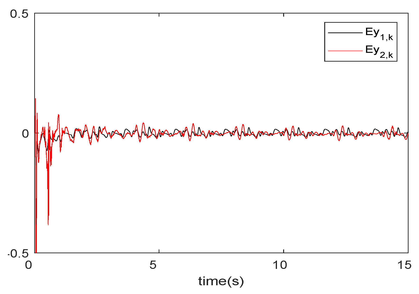
4. Analysis of Experimental Results

In this paper, a second-order unknown discrete-time nonlinear system is considered, and three simulation examples are performed. In order to indicate the effectiveness of the IC estimator, in the first simulation example, $f(y_k,y_{k-1})=0$; in the second simulation example, the proposed data-driven algorithm based on the IC estimator and ReOS-ELM is compared with the MFAC algorithm based on RLS ([31], Equation 5.49); in the third example, the performance of ReOS-ELM when the training data contains noise is compared with ReOS-ELM when the training data does not contain noise, by approaching a nonlinear function.

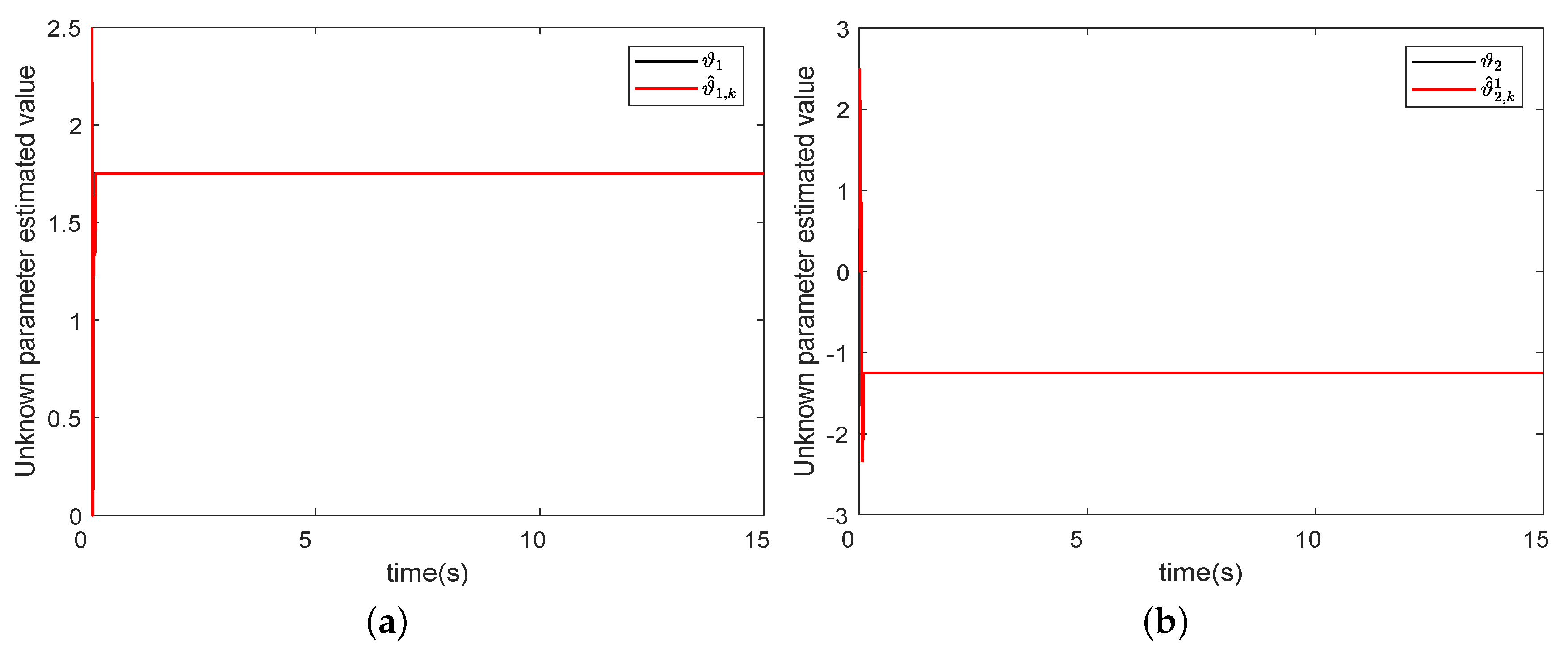
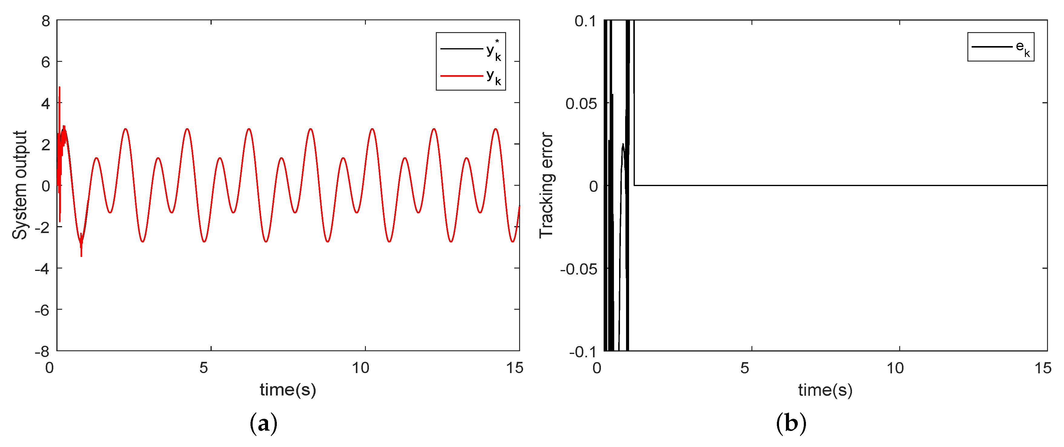
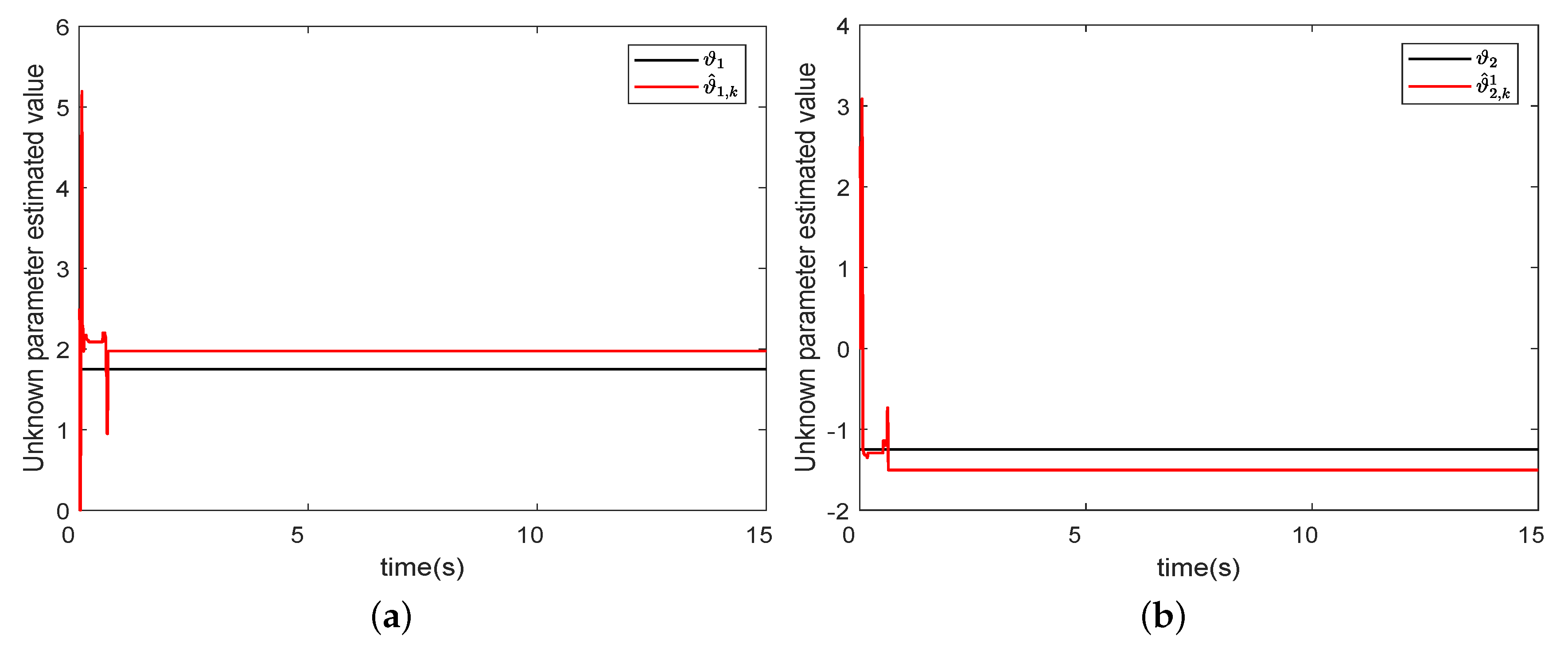
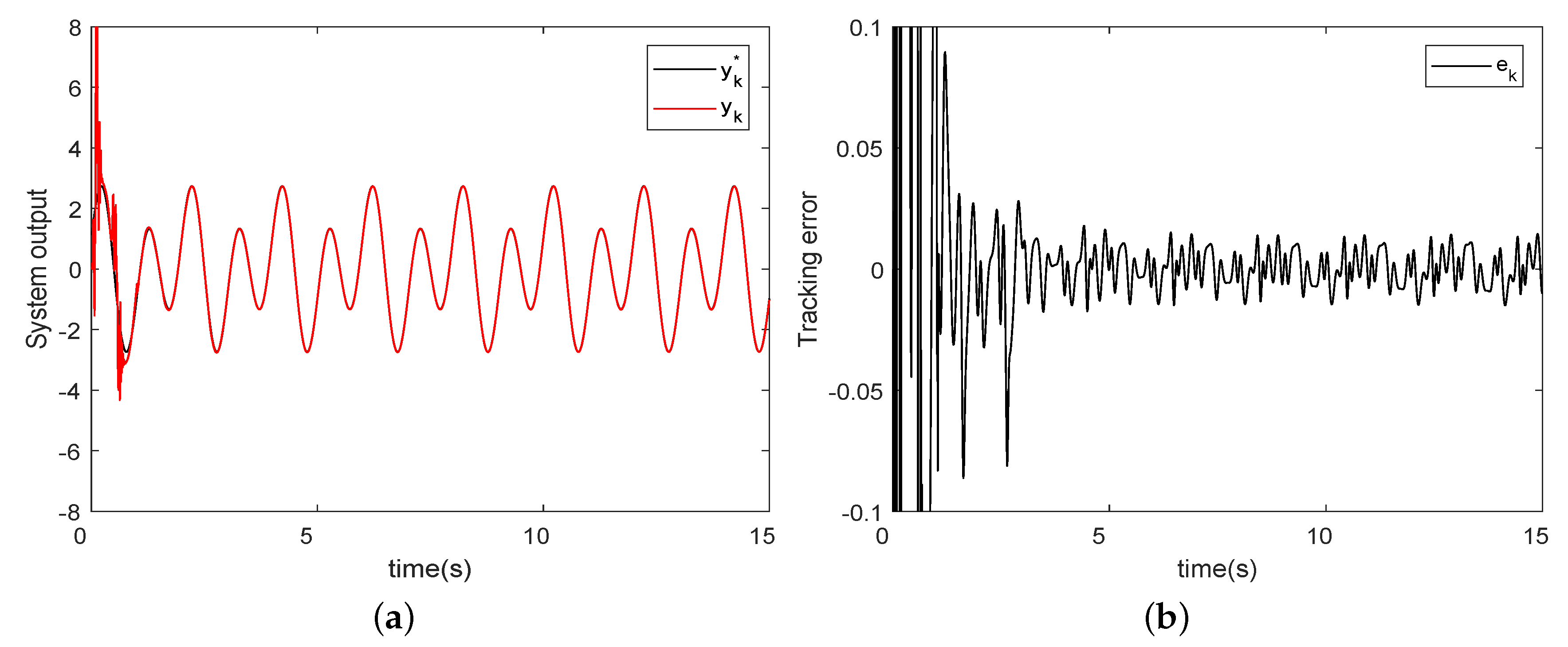
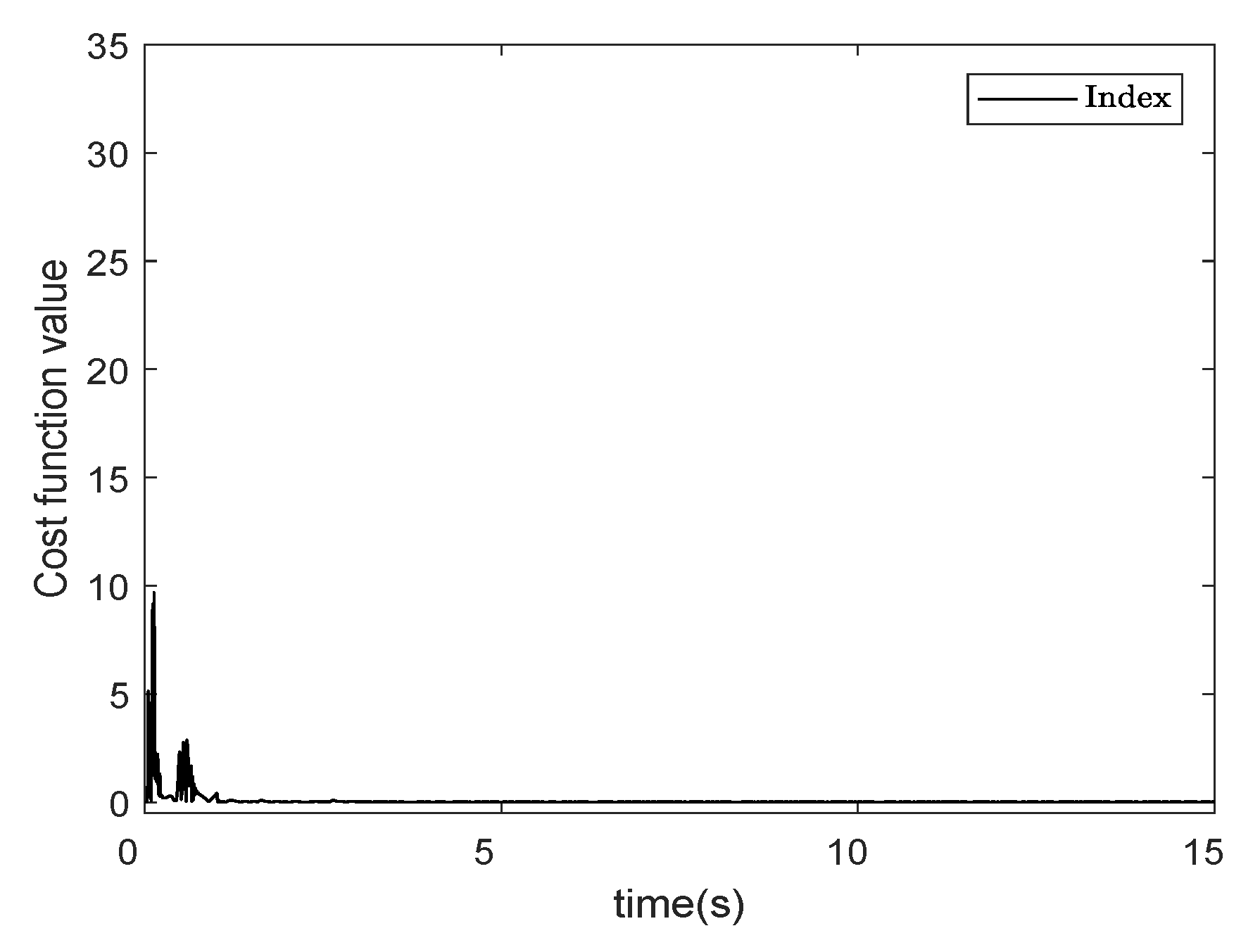
4.1. The First Simulation Example

In this first example, the parameters of the system (16) are

$${\vartheta }_1=1.75,{\vartheta }_2=-1.25,f(y_k,y_{k-1})=0$$

(57)

In this example, the a priori knowledge is listed as follows:

$$L_M=1.5,L_c=0.5$$

(58)

and

$$\begin{array}{cc}\hfill & {\underline{B}}_{\theta ,1}=-10,{\overline{B}}_{\theta ,1}=10\hfill \\ \hfill & {\underline{B}}_{\theta ,2}=-10,{\overline{B}}_{\theta ,2}=15\hfill \end{array}$$

(59)

The desired reference signal $y_{k+1}^{*}$ is

$$y_{k+1}^{*}=2\sin \left(2\pi k{T}_s\right)+1.5\cos \left(\pi k{T}_s\right)$$

(60)

For ReOS-ELM, these parameters are: the number of hidden nodes of ReOS-ELM is $L=25$, $\lambda =0.001$, the activation function of ReOS-ELM is sigmoid, $T_s=0.01$, and $▵=0.15$. The main results, which include the estimated values of $\mathsf{\theta }$ by the improved IC estimator and the tracking error, are depicted in Figure 3 and Figure 4. The curves in Figure 3a,b show the change trends and and estimated values of ${\vartheta }_1$ and ${\vartheta }_2$, respectively. The tracking curves and tracking error are shown in Figure 4a and Figure 4b, respectively. The estimated values shown in Figure 3 show that the values of $\mathsf{\theta }$ estimated by the improved IC effectively approach the actual value, and the small tracking error in Figure 4b also indicates its effective performance in estimating the unknown parameters.

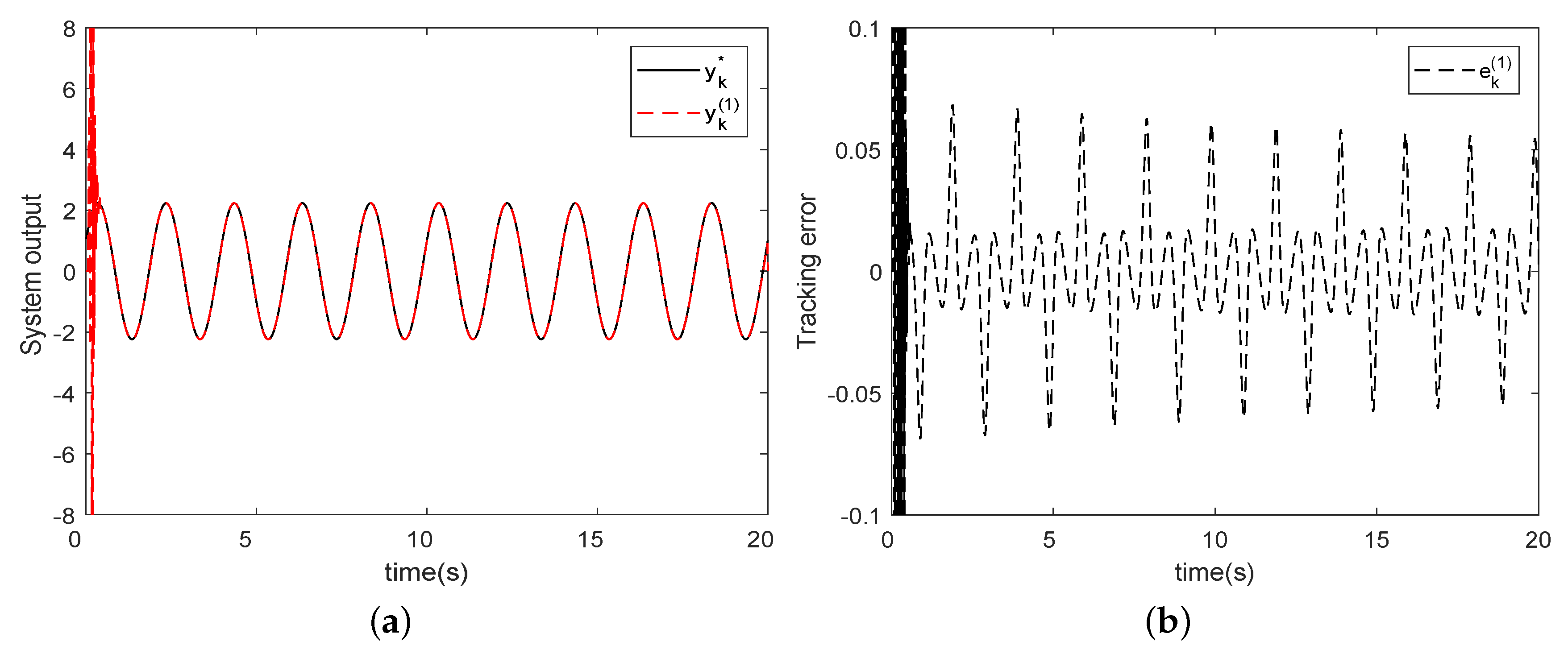
4.2. The Second Simulation Example

The proposed data-driven algorithm based on the IC estimator and ReOS-ELM is a novel kind of DDC method. In order to verify its performance, it is compared with the controller of MFAC based on RLS ([31], Equation 5.49) for a second-order unknown discrete-time nonlinear system which contains a parametric uncertainty part and a nonparametric uncertainty part. In this simulation example,

$$\begin{array}{c}\hfill f(y_k,y_{k-1},u_k)=0.5y_k\sin \left({\log }_{\mathrm{e}}^{10\left|y_{k-1}\right|+1}\right)+0.3y_{k-1}\sin \left({\log }_{\mathrm{e}}^{10\left|y_k\right|+1}\right)\end{array}$$

(61)

In order to check the learning performance of ReOS-ELM in the proposed data-driven control algorithm, the following cost function is introduced

$$\parallel {\mathit{H}}_k{\mathit{\beta }}_k-{\mathit{T}}_k{\parallel }^2+\lambda {\parallel {\mathit{\beta }}_k\parallel }^2$$

(62)

Figure 5, Figure 6, Figure 7 and Figure 8 are the second simulation’s example results. Figure 5 plots the change curves of the estimated values ${\widehat{\vartheta }}_{1,k}$ and ${\widehat{\vartheta }}_{2,k}$. In Figure 6, the curves denote the simulation experimental results of the control algorithm based on the proposed IC estimator and ReOS-ELM, and Figure 6a and Figure 6b show the tracking curves and error curve, respectively. The curve in Figure 7 indicates the change trend of the cost function, Equation (62), which diminishes through time. In Figure 8, the curves denote the simulation experimental results of MFAC based on RLS, and the curves in Figure 8a and Figure 8b show the output signal and error signal, respectively. The change trends of Figure 6b and Figure 8b show that when this system reaches a stable state, the maximum error in the control algorithm based on the proposed IC estimator and ReOS-ELM is 0.0152, the maximum error in MFAC based on RLS is 0.0596. This result indicates that the performance of the proposed algorithm is better than the performance of the MFAC based on RLS. The change curves in Figure 5 show that the final estimated values ${\widehat{\vartheta }}_{1,k}$ and ${\widehat{\vartheta }}_{2,k}$ have some degree of deviation from the values ${\vartheta }_1$ and ${\vartheta }_2$, and it indicates that the semi-parametric model is established depending on the historical data and is different from mechanism models.

4.3. The Third Simulation Example

In order to analyze the influence caused by noise in the training data, two estimated errors of Equation (61) were compared, one is the estimated error by ReOS-ELM in which the training data do not contain noise, and the other is the estimated error by ReOS-ELM in which the training data contain random noise whose range is [−0.2, 0.2]. The errors are shown in Figure 9, which indicates that the noise in the training data would make the estimated error become large, but would not change the performance of approaching Equation (61).

5. Conclusions

In this paper, first, an improved IC estimator is introduced. This improved IC estimator adopts a constraint form which consists of two steps of history data. This is different from the previous results, and the previous results need one step history data. This improvement makes this estimator fit in more systems, and those systems do not need to meet the assumption that the nonparametric uncertainty part of actual systems is bounded. Second, a data-driven control algorithm based on an improved IC estimator and ReOS-ELM is designed. For stability analysis of control systems, a binary updating algorithm of ReOS-ELM is introduced, and the stability of the proposed data-driven control algorithm is guaranteed by a theoretical analysis based on a Lyapunov candidate function. Finally, in order to indicate the effectiveness of the IC estimator, an ideal second-order unknown discrete-time linear system is considered, and the experimental results show that the proposed IC estimator is effective in estimating the unknown parameters of a second-order unknown linear system. Furthermore, the proposed data-driven algorithm is compared with the MFAC based on RLS ([31], Equation 5.49) for the system (16), and the second simulation’s results show that the maximum tracking error in the control algorithm based on the proposed IC estimator and ReOS-ELM is smaller than the maximum tracking error in MFAC based on RLS, which indicates that the proposed data-driven algorithm is effective at improving the control accuracy.

The contribution of this paper is that a novel data-driven control algorithm is introduced, and the stability of this algorithm is guaranteed by theoretical analysis. A semi-parametric model divides a system into a parametric uncertainty part and a nonparametric uncertainty part, and this is different from previous methods, which consider the whole system almost as a black-box model. A semi-parametric model only needs a neural network to estimate the nonparametric uncertainty part rather than the whole system, and this may contribute to reducing the network complexity and calculation workload. However, if the parametric uncertainty part and nonparametric uncertainty part of a semi-parametric model are simultaneously unknown, it is challenging to make use of this model. The proposed data-driven control algorithm can estimate parametric uncertainty part, firstly. Then training data of ReOS-ELM network is obtained, based on symmetry, and the training of ReOS-ELM network and the estimate of nonparametric uncertainty part using ReOS-ELM network are carried out online, successively. The proposed data-driven control algorithm provides a possibility of making use of this model. This algorithm may be used in second-order systems, such as motor control systems. The disadvantage of the proposed data-driven control algorithm is that it is only suitable for second-order systems. The improved IC estimator adopts a polygon to indicate the possible domain of the unknown parameters of the parametric uncertainty part, and this polygon can only indicate those data which belong to it. Because of the nature of the polygon, the improved IC estimator is not suitable for higher-order systems. In future research, the IC estimator may be improved by changing the way in which it is used in the possible domain of the unknown parameters of the parametric uncertainty part, for example, for third-order systems a cube may be adopted to indicate those data which belong to it. For higher-order systems, it is a challenging thing to indicate the possible domain of unknown parameters by using geometry knowledge. However, with the developments of computer technology and parallel computing, there may be some solutions by estimating the unknown parameters of the parametric uncertainty part in parallel.

References

1. Hou, Z.; Jin, S. A novel data-driven control approach for a class of discrete-time nonlinear systems. IEEE Trans. Control Sytems Technol. 2011, 19, 1549–1558. [Google Scholar] [CrossRef]
2. Liao, Y.; Du, T.; Jiang, Q. Model-free adaptive control method with variable forgetting factor for unmanned surface vehicle control. Appl. Ocean. Res. 2019, 93, 101945. [Google Scholar] [CrossRef]
3. Hou, Z.; Zhu, Y. Controller-Dynamic-Linearization-Based Model Free Adaptive Control for Discrete-Time Nonlinear Systems. IEEE Trans. Ind. Inform. 2013, 9, 2301–2309. [Google Scholar] [CrossRef]
4. Aghaei Hashjin, S.; Pang, S.; Ait-Abderrahim, K.; Nahid-Mobarakeh, B. Data-Driven Model-Free Adaptive Current Control of a Wound Rotor Synchronous Machine Drive System. IEEE Trans. Transp. Electrif. 2020, 6, 1146–1156. [Google Scholar] [CrossRef]
5. Zhang, X.; Ma, H. Data-Driven Model-Free Adaptive Control Based on Error Minimized Regularized Online Sequential Extreme Learning Machine. Energies 2019, 12, 3241. [Google Scholar] [CrossRef]
6. Yu, M.; Zhou, W.; Liu, B. On iterative learning control for MIMO nonlinear systems in the presence of time-iteration-varying parameters. Nonlinear Dyn. 2017, 89, 2561–2571. [Google Scholar] [CrossRef]
7. He, W.; Meng, T.; He, X.; Ge, S.S. Unified iterative learning control for flexible structures with input constraints. Automatica 2018, 96, 326–336. [Google Scholar] [CrossRef]
8. Mandra, S.; Galkowski, K.; Rogers, E.; Rauh, A.; Aschemann, H. Performance-enhanced robust iterative learning control with experimental application to PMSM position tracking. IEEE Trans. Control Syst. Technol. 2019, 27, 1813–1819. [Google Scholar] [CrossRef]
9. Choi, W.; Volpe, F.A. Simultaneous iterative learning control of mode entrainment and error field. Nucl. Fusion 2019, 59, 056011. [Google Scholar] [CrossRef]
10. Hjalmarsson, H. Iterative feedback tuning—An overview. Int. J. Adapt. Control Signal Process. 2002, 16, 373–395. [Google Scholar] [CrossRef]
11. Heertjes, M.F.; Vander Velden, B.; Oomen, T. Constrained iterative feedback tuning for robust control of a wafer stage system. IEEE Trans. Control Syst. Technol. 2016, 24, 56–66. [Google Scholar] [CrossRef]
12. Sanchez Pena, R.S.; Colmegna, P.; Bianchi, F. Unfalsified control based on the controller parameterisation. Int. J. Syst. Sci. 2015, 46, 2820–2831. [Google Scholar] [CrossRef]
13. Safonov, M.; Tsao, T. The unfalsified control concept and learning. IEEE Trans. Autom. Control 1997, 42, 843–847. [Google Scholar] [CrossRef]
14. Jeng, J.C.; Lin, Y.W. Data-driven nonlinear control design using virtual-reference feedback tuning based on the block-oriented modeling of nonlinear systems. Ind. Eng. Chem. Res. 2018, 57, 7583–7599. [Google Scholar] [CrossRef]
15. Kobayashi, M.; Konishi, Y.; Ishigaki, H. A lazy learning control method using support vector regression. Int. J. Innovtive Comput. Inf. Control 2007, 3, 1511–1523. [Google Scholar]
16. Jia, C.; Li, X.; Wang, K.; Ding, D. Adaptive control of nonlinear system using online error minimum neural networks. Isa Trans. 2016, 65, 125–132. [Google Scholar] [CrossRef] [PubMed]
17. Li, X.; Jia, C.; Liu, D.; Ding, D. Adaptive Control of Nonlinear Discrete-Time Systems by Using OS-ELM Neural Networks. Abstr. Appl. Anal. 2014, 2014, 1–11. [Google Scholar] [CrossRef]
18. Rahmani, B.; Belkheiri, M. Adaptive neural network output feedback control for flexible multi-link robotic manipulators. Int. J. Control 2019, 92, 2324–2338. [Google Scholar] [CrossRef]
19. Li, X.; Fang, J.; Li, H. Exponential stabilisation of memristive neural networks under intermittent output feedback control. Int. J. Control 2018, 91, 1848–1860. [Google Scholar] [CrossRef]
20. Chen, C.; Modares, H.; Xie, K.; Lewis, F.L.; Wan, Y.; Xie, S. Reinforcement Learning-based Adaptive Optimal Exponential Tracking Control of Linear Systems with Unknown Dynamics. IEEE Trans. Autom. Control 2024. to be published. [Google Scholar] [CrossRef]
21. Nguyen, N.D.; Nguyen, T.; Nahavandi, S. Multi-agent behavioral control system using deep reinforcement learning. Neurocomputing 2019, 359, 58–68. [Google Scholar] [CrossRef]
22. Wang, Z.; Li, H.; Wang, J.; Shen, F. Deep reinforcement learning based conflict detection and resolution in air traffic control. IET Intell. Transp. Syst. 2019, 13, 1041–1047. [Google Scholar] [CrossRef]
23. Khalatbarisoltani, A.; Soleymani, M.; Khodadadi, M. Online control of an active seismic system via reinforcement learning. Struct. Control Health Monit. 2019, 26, e2298. [Google Scholar] [CrossRef]
24. Yang, X.; Liu, D.; Wang, D. Reinforcement learning for adaptive optimal control of unknown continuous-time nonlinear systems with input constraints. Int. J. Control 2014, 87, 553–566. [Google Scholar] [CrossRef]
25. Ma, H.; Lum, K.Y.; Ge, S.S. Adaptive control for a discrete-time first-order nonlinear system with both parametric and non-parametric uncertainties. In Proceedings of the IEEE Conference on Decision & Control, New Orleans, LA, USA, 12–14 December 2007. [Google Scholar]
26. Zhou, H.; Ma, H.; Li, N.; Yang, C. Semi-parametric adaptive control of discrete-time systems using extreme learning machine. In Proceedings of the 2017 9th International Conference on Modelling, Identification and Control (ICMIC 2017), Piscataway, NJ, USA, 26–28 July 2017. [Google Scholar]
27. Zhang, X.; Ma, H.; Luo, M.; Liu, X. Adaptive sliding mode control with information concentration estimator for a robot arm. Int. J. Syst. Sci. 2020, 51, 217–228. [Google Scholar] [CrossRef]
28. Huang, G.B.; Zhu, Q.Y.; Siew, C.K. Extreme learning machine: Theory and applications. Neurocomputing 2006, 70, 489–501. [Google Scholar] [CrossRef]
29. Liang, N.Y.; Huang, G.B.; Saratchandran, P.; Sundararajan, N. A fast and accurate online sequential learning algorithm for feedforward networks. IEEE Trans. Neural Netw. 2006, 17, 1411–1423. [Google Scholar] [CrossRef]
30. Huynh, H.T.; Won, Y. Regularized online sequential learning algorithm for single-hidden layer feedforward neural networks. Pattern Recognit. Lett. 2011, 32, 1930–1935. [Google Scholar] [CrossRef]
31. Hou, Z. Nonparametric Model and Adaptive Control Theory, 1st ed.; Science Press of China: Beijing, China, 1999. [Google Scholar]
Figure 1. The process of the IC estimator at time k, the polygon v indicates the possible candidate regions of unknown parameters at the previous moment. The straight line comes from the information at step k; it splits v into two sub-polygons, the left-hand one of which will become the new polygon v . Four typical situations of IC estimator are shown in subfigures (a), (b), (c) and (d), respectively.
Symmetry 16 00088 g001
Figure 2. The process of the proposed data-driven control algorithm. The green area indicates the initialization stage and the yellow area indicates the parameter learning stage.
Symmetry 16 00088 g002
Figure 3. The estimated values of θ by the improved IC estimator in the first simulation example. ϑ 1 and ϑ 2 are two actual values of θ , and the estimated curves ϑ ^ 1 , k and ϑ ^ 2 , k are shown in (a) and (b), respectively.
Symmetry 16 00088 g003
Figure 4. The performance of the control system in the first simulation example. (a) and (b) show the tracking curves and error curve, respectively.
Symmetry 16 00088 g004
Figure 5. The estimated values of θ by the improved IC estimator in the second simulation. ϑ 1 and ϑ 2 are two actual values of θ . The estimated curves ϑ ^ 1 , k and ϑ ^ 2 , k are shown in (a) and (b), respectively.
Symmetry 16 00088 g005
Figure 6. The results of the proposed novel data-driven control algorithm based on the IC estimator and ReOS-ELM in the second simulation example. (a) and (b) show the tracking curves and error curve, respectively.
Symmetry 16 00088 g006
Figure 7. Cost function change curve.
Symmetry 16 00088 g007
Figure 8. The results of the MFAC algorithm based on RLS in the second simulation example. (a) and (b) show the tracking curves and error curve, respectively.
Symmetry 16 00088 g008
Figure 9. Two estimated errors of Equation (61). E y 1 , k indicates the estimated error by ReOS-ELM in which the training data does not contain noise, and E y 2 , k indicates the estimated error by ReOS-ELM in which the training data contains random noise whose range is [−0.2, 0.2].
Symmetry 16 00088 g009
Disclaimer/Publisher’s Note: The statements, opinions and data contained in all publications are solely those of the individual author(s) and contributor(s) and not of MDPI and/or the editor(s). MDPI and/or the editor(s) disclaim responsibility for any injury to people or property resulting from any ideas, methods, instructions or products referred to in the content.