On a Hierarchy of Vector Derivative Nonlinear Schrödinger Equations

Abstract

We propose a new hierarchy of the vector derivative nonlinear Schrödinger equations and consider the simplest multiphase solutions of this hierarchy. The study of the simplest solutions of these equations led to the following results. First, the three-leaf spectral curves $\Gamma =\left\{\right(\mu ,\lambda \left)\right\}$ of the simplest multiphase solutions have a quite simple symmetry. They are invariant with respect to holomorphic involution $\tau$. The type of this involution depends on the genus of the spectral curve. Or the involution has the form $\tau :(\mu ,\lambda )\to (\mu ,-\lambda )$, or $\tau :(\mu ,\lambda )\to (-\mu ,-\lambda )$. The presence of symmetry leads to the fact that the dynamics of the solution is determined not by the entire spectral curve $\Gamma$, but by its factor $\Gamma /\tau$, which has a smaller genus. Secondly, it turned out that the dynamics of the two-component vector $\mathbf{p}={(p_1,p_2)}^t$ is determined, first of all, by the dynamics of its length $\left|\mathbf{p}\right|$. Independent equations determine the dependence of the direction of the vector $\mathbf{p}$ from its length. In cases where the direction of the vector $\mathbf{p}$ is fixed, the corresponding spectral curve splits into separate components. In conclusion, we note that, as in the case of the Manakov system, the equation of the spectral curve is invariant with respect to the orthogonal transformation of the vector solutions. I.e., the solution can be found from the spectral curve up to the orthogonal transformation. This fact indicates that the spectral curve does not depend on the individual components of the solution, but on their symmetric functions. Thus, the spectral data of multiphase solutions have two symmetries. These symmetries make it difficult to reconstruct signals from their spectral data. The work contains examples illustrating these statements.

1. Introduction

Vector integrable nonlinear equations still continue to attract active attention (see, for example, [1,2,3,4,5,6,7,8,9,10]). Mainly, the vector nonlinear Schrödinger equation is considered. Much less work is devoted to the derivative form of the vector equation (see, for example, [11,12,13,14,15,16,17,18,19]). Scalar forms of the derivative nonlinear Schrödinger equation are given much more attention (see, for example, [20,21,22,23,24,25]). Note that for each derivative nonlinear Schrödinger equation, its vector form is obtained, and multi-soliton solutions of these vector forms are investigated. Attention to two-component variants of the nonlinear Schrodinger equation is due to the fact that with the help of double-polarized waves, twice as much information can be transmitted over an optical fiber [26,27,28,29]. In practice, it turns out that it is much more difficult to recover encoded information from a two-component signal. Apparently, this is due to the results obtained in our work. When transmitting information, it is assumed that each component is independent and carries its own part of the information. As we proved earlier [30], the spectral curve is invariant with respect to the orthogonal transformation of the solution. I.e., it does not depend on the individual components of the solution, but on their symmetric functions. This statement is also true for the equations from our current work. This is one of the possible reasons for the difficulty of recovering information from the transmitted signal. The second possible reason most likely follows from the fact that the spectral curve corresponding to a solution with linearly dependent components is greatly reduced. The correctness of this statement can be seen in the examples from this work. Therefore, when transmitting signals that differ slightly from each other, some information about the spectral characteristics of the signals may be lost. In addition, as our examples show, the genus of the spectral curve far exceeds the number of phases of the solution. Thus, part of the spectral data is redundant. Also, as we show, in the case of the vector equations, first of all, we get the law of transformation of the length of the solution vector, and then the rule of direction transformation. When replacing the components of a vector by its length and vice versa, information loss may occur. Thus, based on the results of this work, we can advise transmitting information not in Cartesian coordinates, but in polar ones.

In this paper, we use the monodromy matrix method (see, for example, [1,20,30]) to construct a hierarchy of the Gerdjikov–Ivanov vector equation and investigate the simplest solutions of equations from this hierarchy. As a rule, in the works devoted to the study of vector nonlinear equations, the individual components of the vector are analyzed. At the same time, sometimes there are works (see, for example, [7]) in which the behavior of the length and tangent of the angle of inclination of the vector is investigated. Our studies of the simplest solutions have shown that in the case of a vector nonlinear equation, the evolution of a vector can naturally be divided into two components: the evolution of the length of the vector and the evolution of its direction. Note that this statement is also true for the Manakov system, which can be seen by looking at the calculations in [1]. For example, assuming

$$p_1=\left|\mathbf{p}\right|e^{i{\alpha }_1}cos\left(\varphi \right),p_2=\left|\mathbf{p}\right|e^{i{\alpha }_2}sin\left(\varphi \right)$$

and $\mathbf{q}=\sigma {\mathbf{p}}^{*}$, where $\sigma =\pm 1$, we have

$$u_1=p_1{q}_1={\sigma \left|\mathbf{p}\right|}^2{cos}^2\left(\varphi \right),u_2=p_2{q}_2=\sigma {\left|\mathbf{p}\right|}^2{sin}^2\left(\varphi \right)$$

(1)

and

$$\begin{array}{cc}\hfill & u=u_1+u_2=\sigma {\left|\mathbf{p}\right|}^2,\hfill \\ \hfill & v=u_1-u_2=\sigma {\left|\mathbf{p}\right|}^{2}cos\left(2\varphi \right),\hfill \\ \hfill & \widehat{v}=v/u=cos\left(2\varphi \right)\le 1.\hfill \end{array}$$

(2)

If the reduction has the form

$$q_1=\sigma p_1^{*},q_2=-\sigma p_2^{*},$$

(3)

then the angle $\varphi$ becomes purely imaginary $\varphi =i\widehat{\varphi }$, where $\widehat{\varphi }\in \mathbb{R}$. In this case, the “direction” of the vector $\mathbf{p}$ is defined by the function $\widehat{v}=cosh\left(2\widehat{\varphi }\right)\ge 1$. Thus, if $\widehat{v}<1$, then it is possible to construct solutions that satisfy the reduction $\mathbf{q}=\sigma {\mathbf{p}}^{*}$. If $\widehat{v}>1$, then the solutions will satisfy the reduction (3). When $\widehat{v}=1$, the second component of the vector $\mathbf{p}$ is missing ($u_2=0$). The reduction sign $\sigma$ is determined by the sign of the function u:

$$\sigma =\mathrm{sign}\left(u\right).$$

Note that the functions u, v, and $\widehat{v}$ naturally appear during calculations. Also, note that from Equation (1) it follows that $|p_j|=\sqrt{|u_j|}$. Therefore, to plot the amplitudes of the individual components $p_j$ of the vector $\mathbf{p}$, it is enough to find $u_j$. The analysis of the examples showed that when the direction of the vector $\mathbf{p}$ is independent of the coordinate and time ($\widehat{v}=const$), the spectral curve splits into two separate components, and the dynamics of the solution is determined by a spectral curve of a smaller kind than in the case when the direction of the vector $\mathbf{p}$ changes depending on the coordinate and time.

The presented article consists of an introduction, four sections, and concluding remarks. In the first section, we define the Lax operator, define the monodromy matrix, find recurrent relations between its elements, and derive the equation of spectral curves associated with multiphase solutions. In Section 2, we define the second Lax pair operators and obtain vector integrable nonlinear differential equations from the hierarchy of the Gerdjikov–Ivanov vector equation. The first equations from this hierarchy have the form

$$\begin{array}{cc}\hfill & i{\mathbf{p}}_{t_1}-{\mathbf{p}}_{xx}+2i\left({\mathbf{p}}^t{\mathbf{q}}_x\right)\mathbf{p}-2{\left({\mathbf{p}}^t\mathbf{q}\right)}^2\mathbf{p}=0,\hfill \\ \hfill & i{\mathbf{q}}_{t_1}+{\mathbf{q}}_{xx}+2i\left({\mathbf{q}}^t{\mathbf{p}}_x\right)\mathbf{q}+2{\left({\mathbf{p}}^t\mathbf{q}\right)}^2\mathbf{q}=0\hfill \end{array}$$

and

$$\begin{array}{cc}\hfill & {\mathbf{p}}_{t_2}+{\mathbf{p}}_{xxx}-3i\left({\mathbf{p}}_x^t{\mathbf{q}}_x\right)\mathbf{p}-3i\left({\mathbf{p}}^t{\mathbf{q}}_x\right){\mathbf{p}}_x+3\left({\mathbf{p}}^t\mathbf{q}\right)\left({\mathbf{p}}_x^t\mathbf{q}\right)\mathbf{p}+3{\left({\mathbf{p}}^t\mathbf{q}\right)}^2{\mathbf{p}}_x=0,\hfill \\ \hfill & {\mathbf{q}}_{t_2}+{\mathbf{q}}_{xxx}+3i\left({\mathbf{p}}_x^t{\mathbf{q}}_x\right)\mathbf{q}+3i\left({\mathbf{q}}^t{\mathbf{p}}_x\right){\mathbf{q}}_x+3\left({\mathbf{p}}^t\mathbf{q}\right)\left({\mathbf{q}}_x^t\mathbf{p}\right)\mathbf{q}+3{\left({\mathbf{p}}^t\mathbf{q}\right)}^2{\mathbf{q}}_x=0.\hfill \end{array}$$

If we replace vectors with scalars in these equations, we obtain the Gerdjikov–Ivanov equation and one of the forms of the mKdV equation.

In Section 3, we consider solutions in the form of plane waves. We show that there are two types of plane waves that differ in the properties of their spectral curves. If $\mathbf{p}(x,t)=p(x,t)\mathbf{k}$, where $\mathbf{k}$ is a constant vector, then the equation of the spectral curve does not depend on the direction of the vector $\mathbf{p}$, in another case, the equation of the spectral curve depends on the direction of the vector $\mathbf{p}$. In the case when the direction of the vector $\mathbf{p}$ is fixed, the corresponding spectral curve splits into separate components.

In the fourth section, the simplest nontrivial solutions of the Gerdjikov–Ivanov vector equation are investigated. In this case, the function u is an elliptic function or its degeneracy, and the function $\widehat{v}$ depends on the function u according to the following formula:

$$\widehat{v}=Asin\left(\kappa (\theta +t_1)\right)+B,$$

where ${\partial }_x\theta =\pm u^{-1}$. Note that the simplest nontrivial solutions are also divided into two types. If $A=0$, then the direction of the vector $\mathbf{p}$ is fixed, only its length changes. The spectral curve of such a solution also splits into two components. If $A\ne 0$, then the vector makes small fluctuations near the direction given by the equality $\widehat{v}=B$. The amplitude of these oscillations satisfies the condition $\left|A\right|<\left|\left|B\right|-1\right|$. Therefore, if $\left|B\right|<1$, then $|\widehat{v}| < 1$, and from $\left|B\right|>1$ follows the inequality $|\widehat{v}| > 1$.

2. The Monodromy Matrix

Let the Lax operator have the form

$$i{\Psi }_x=U\Psi ,$$

(4)

where

$$\begin{array}{c}U=-{\lambda }^{2}J+\lambda Q+R,\end{array}$$

(5)

$$\begin{array}{c}J={\displaystyle \frac{1}{3}}\left(\begin{array}{ccc}2& 0& 0\\ 0& -1& 0\\ 0& 0& -1\end{array}\right),Q=\left(\begin{array}{cc}0& {\mathbf{p}}^t\\ -\mathbf{q}& \mathbf{0}\end{array}\right),R=\left(\begin{array}{cc}-{\mathbf{p}}^t\mathbf{q}& {\mathbf{0}}^t\\ \mathbf{0}& \mathbf{q}{\mathbf{p}}^t\end{array}\right),\end{array}$$

(6)

${\mathbf{p}}^t=(p_1,p_2)$, ${\mathbf{q}}^t=(q_1,q_2)$.

Let us consider Equations (4) and (5) with matrices (6). The monodromy matrix M is a polynomial of the spectral parameter $\lambda$, and satisfies the equation (see, for example, [1,31])

$$i{M}_x+MU-UM=\mathbf{0}$$

(7)

From Equation (7), the following structure of the matrix M follows:

$$M=V_n+\sum _{k=1}^{n-1}{c}_k{V}_{n-k}+c_{n}U+c_{n+1}{V}_{-1}+J_n,$$

(8)

where $V_1=\lambda U+V_1^0$, $V_{j+1}=\lambda V_j+V_{j+1}^0$, $V_{-1}=-\lambda J+Q$,

$$\begin{array}{c}{V}_{2k-1}^0=\left(\begin{array}{cc}0& {\mathbf{H}}_k^t\\ {\mathbf{G}}_k& \mathbf{O}\end{array}\right),V_{2k}^0=\left(\begin{array}{cc}-{\mathcal{F}}_k& {\mathbf{0}}^t\\ \mathbf{0}& F_k\end{array}\right),{\mathcal{F}}_k=\mathrm{Tr}{F}_k,k\ge 1,\\ J_n=\left(\begin{array}{ccc}-2c_{n+2}& 0& 0\\ 0& c_{n+2}+c_{n+3}& c_{n+4}\\ 0& c_{n+5}& c_{n+2}-c_{n+3}\end{array}\right).\end{array}$$

The elements of the matrix $V_k^0$ satisfy the following recurrence relations

$$\begin{array}{cc}\hfill & {\mathbf{H}}_1=-i{\mathbf{p}}_x,{\mathbf{G}}_1=-i{\mathbf{q}}_x,\hfill \\ \hfill & {\mathbf{H}}_{k+1}=\left(F_k^t+{\mathcal{F}}_{k}I\right)\mathbf{p}-\left(\mathbf{p}{\mathbf{q}}^t+\left({\mathbf{p}}^t\mathbf{q}\right)I\right){\mathbf{H}}_k-i{\partial }_x{\mathbf{H}}_k,\hfill \\ \hfill & {\mathbf{G}}_{k+1}=-\left(F_k+{\mathcal{F}}_{k}I\right)\mathbf{q}-\left(\mathbf{q}{\mathbf{p}}^t+\left({\mathbf{q}}^t\mathbf{p}\right)I\right){\mathbf{G}}_k+i{\partial }_x{\mathbf{G}}_k,\hfill \\ \hfill & {\partial }_x{F}_k=\mathbf{q}{\partial }_x{\mathbf{H}}_k^t-{\partial }_x{\mathbf{G}}_k{\mathbf{p}}^t-i\left(\mathbf{q}{\mathbf{p}}^t+\left({\mathbf{q}}^t\mathbf{p}\right)I\right){\mathbf{G}}_k{\mathbf{p}}^t\hfill \\ \hfill & -i\mathbf{q}{\mathbf{H}}_k^t\left(\mathbf{q}{\mathbf{p}}^t+\left({\mathbf{q}}^t\mathbf{p}\right)I\right).\hfill \end{array}$$

(9)

In particular,

$$\begin{array}{cc}\hfill & F_1=i\left({\mathbf{q}}_x{\mathbf{p}}^t-\mathbf{q}{\mathbf{p}}_x^t\right)-{\left(\mathbf{q}{\mathbf{p}}^t\right)}^2,\hfill \\ \hfill & {\mathcal{F}}_1=i\left({\mathbf{p}}^t{\mathbf{q}}_x-{\mathbf{q}}^t{\mathbf{p}}_x\right)-{\left({\mathbf{p}}^t\mathbf{q}\right)}^2,\hfill \\ \hfill & H_2=-{\mathbf{p}}_{xx}+2i\left({\mathbf{p}}^t{\mathbf{q}}_x\right)\mathbf{p}-2{\left({\mathbf{p}}^t\mathbf{q}\right)}^2\mathbf{p},\hfill \\ \hfill & G_2={\mathbf{q}}_{xx}+2i\left({\mathbf{q}}^t{\mathbf{p}}_x\right)\mathbf{q}+2{\left({\mathbf{p}}^t\mathbf{q}\right)}^2\mathbf{q},\hfill \\ \hfill & F_2=-2{\left(\mathbf{q}{\mathbf{p}}^t\right)}^3-(\mathbf{q}{\mathbf{p}}_{xx}^t+{\mathbf{q}}_{xx}{\mathbf{p}}^t)+{\mathbf{q}}_x{\mathbf{p}}_x^t\hfill \\ \hfill & -i\left({\mathbf{p}}_x^t{s}_0\mathbf{p}\right)\mathbf{q}{\mathbf{q}}^t{s}_0+i\left({\mathbf{q}}^t{s}_0{\mathbf{q}}_x\right)s_0\mathbf{p}{\mathbf{p}}^t,\hfill \\ \hfill & {\mathcal{F}}_2=-2{\left({\mathbf{p}}^t\mathbf{q}\right)}^3-({\mathbf{q}}^t{\mathbf{p}}_{xx}+{\mathbf{p}}^t{\mathbf{q}}_{xx})+{\mathbf{p}}_x^t{\mathbf{q}}_x,\hfill \\ \hfill & H_3=i{\mathbf{p}}_{xxx}+3\left({\mathbf{p}}_x^t{\mathbf{q}}_x\right)\mathbf{p}+3\left({\mathbf{p}}^t{\mathbf{q}}_x\right){\mathbf{p}}_x+3i\left({\mathbf{p}}^t\mathbf{q}\right)\left({\mathbf{p}}_x^t\mathbf{q}\right)\mathbf{p}+3i{\left({\mathbf{p}}^t\mathbf{q}\right)}^2{\mathbf{p}}_x,\hfill \\ \hfill & G_3=i{\mathbf{q}}_{xxx}-3\left({\mathbf{p}}_x^t{\mathbf{q}}_x\right)\mathbf{q}-3\left({\mathbf{q}}^t{\mathbf{p}}_x\right){\mathbf{q}}_x+3i\left({\mathbf{p}}^t\mathbf{q}\right)\left({\mathbf{q}}_x^t\mathbf{p}\right)\mathbf{q}+3i{\left({\mathbf{p}}^t\mathbf{q}\right)}^2{\mathbf{q}}_x,\hfill \end{array}$$

where

$$s_0=\left(\begin{array}{cc}0& 1\\ -1& 0\end{array}\right).$$

From Equation (7), in addition to the recurrent relations (9), stationary equations also follow. Any m-phase solution for $m\le n$ and for all values of t and z satisfies these stationary equations. As in the case of scalar derivative nonlinear Schrödinger equations [20], stationary vector equations form two groups. For $n>1$, stationary vector equations have the form

$$\begin{array}{c}\left(i{\partial }_x{V}_n^0+[V_n^0,R]\right)+\sum _{k=1}^{n-1}{c}_k\left(i{\partial }_x{V}_{n-k}^0+[V_{n-k}^0,R]\right)\hfill \\ \hfill \hspace{1em}\hspace{1em}\hspace{1em}\hspace{1em}\hspace{1em}\hspace{1em}\hspace{1em}\hspace{1em}\hspace{1em}\hspace{1em}\hspace{1em}\hspace{1em}\hspace{1em}\hspace{1em}\hspace{1em}+i{c}_n{\partial }_{x}R+c_{n+1}\left(i{\partial }_{x}Q+[Q,R]\right)+[J_n,R]=\mathbf{0}\end{array}$$

and

$$\begin{array}{c}\left(i{\partial }_x{V}_{n-1}^0+[V_{n-1}^0,R]+[V_n^0,Q]\right)\hfill \\ \hspace{1em}\hspace{1em}\hspace{1em}\hspace{1em}\hspace{1em}\hspace{1em}+\sum _{k=1}^{n-2}{c}_k\left(i{\partial }_x{V}_{n-1-k}^0+[V_{n-1-k}^0,R]+[V_{n-k}^0,Q]\right)\hfill \\ \hspace{1em}\hspace{1em}\hspace{1em}\hspace{1em}\hspace{1em}\hspace{1em}\hspace{1em}\hspace{1em}\hspace{1em}\hspace{1em}\hspace{1em}\hspace{1em}\hspace{1em}+c_{n-1}\left(i{\partial }_{x}R+[V_1^0,Q]\right)+i{c}_n{\partial }_{x}Q+[J_n,Q]=\mathbf{0}.\hfill \end{array}$$

Note that since the structure of matrices $V_n^0$ depends on parity, the scalar stationary equations for even and odd n have a different form. The compatibility of this overridden system of equations imposes restrictions on the constants $c_k$.

Other stationary equations, which are satisfied by multiphase solutions, can be obtained from the equations of the spectral curve. Recall that the equation of the spectral curve of the multiphase solution is the characteristic equation of the monodromy matrix [31]:

$$\Gamma :\mathcal{R}(\mu ,\lambda )=det(\mu I-M)=0.$$

From Formula (8), it follows that the equation of the spectral curve $\Gamma$ has the form

$$\mathcal{R}(\mu ,\lambda )={\mu }^3+\mathcal{A}\left(\lambda \right)\mu +\mathcal{B}\left(\lambda \right)=0,$$

(10)

where

$$\begin{array}{cc}\hfill & \mathcal{A}\left(\lambda \right)=-{\displaystyle \frac{1}{3}}{\lambda }^{2n+4}-{\displaystyle \frac{2c_1}{3}}{\lambda }^{2n+3}+\sum _{k=2}^{2n+4}{A}_k{\lambda }^{2n+4-k},\hfill \\ \hfill & \mathcal{B}\left(\lambda \right)={\displaystyle \frac{2}{27}}{\lambda }^{3n+6}+{\displaystyle \frac{2c_1}{9}}{\lambda }^{3n+5}+\sum _{k=2}^{3n+6}{B}_k{\lambda }^{3n+6-k}.\hfill \end{array}$$

3. Integrable Nonlinear Equations

Let us define the second equation of the Lax pair by the equation

$$i{\Psi }_{t_k}=V_{2k}\Psi .$$

(11)

Then, the following integrable nonlinear evolutionary equations:

$${\mathbf{p}}_{t_k}=i{\mathbf{H}}_{k+1},{\mathbf{q}}_{t_k}=i{\mathbf{G}}_{k+1}$$

(12)

follow from the Lax pair compatibility condition.

Thus, the first equations from this hierarchy have the forms

$$\begin{array}{cc}\hfill & i{\mathbf{p}}_{t_1}-{\mathbf{p}}_{xx}+2i\left({\mathbf{p}}^t{\mathbf{q}}_x\right)\mathbf{p}-2{\left({\mathbf{p}}^t\mathbf{q}\right)}^2\mathbf{p}=0,\hfill \\ \hfill & i{\mathbf{q}}_{t_1}+{\mathbf{q}}_{xx}+2i\left({\mathbf{q}}^t{\mathbf{p}}_x\right)\mathbf{q}+2{\left({\mathbf{p}}^t\mathbf{q}\right)}^2\mathbf{q}=0\hfill \end{array}$$

(13)

and

$$\begin{array}{cc}\hfill & {\mathbf{p}}_{t_2}+{\mathbf{p}}_{xxx}-3i\left({\mathbf{p}}_x^t{\mathbf{q}}_x\right)\mathbf{p}-3i\left({\mathbf{p}}^t{\mathbf{q}}_x\right){\mathbf{p}}_x+3\left({\mathbf{p}}^t\mathbf{q}\right)\left({\mathbf{p}}_x^t\mathbf{q}\right)\mathbf{p}+3{\left({\mathbf{p}}^t\mathbf{q}\right)}^2{\mathbf{p}}_x=0,\hfill \\ \hfill & {\mathbf{q}}_{t_2}+{\mathbf{q}}_{xxx}+3i\left({\mathbf{p}}_x^t{\mathbf{q}}_x\right)\mathbf{q}+3i\left({\mathbf{q}}^t{\mathbf{p}}_x\right){\mathbf{q}}_x+3\left({\mathbf{p}}^t\mathbf{q}\right)\left({\mathbf{q}}_x^t\mathbf{p}\right)\mathbf{q}+3{\left({\mathbf{p}}^t\mathbf{q}\right)}^2{\mathbf{q}}_x=0.\hfill \end{array}$$

(14)

For $p_j(x,t_1)=k_{j}p(x,t_1)$ and $q_j(x,t_1)=k_{j}q(x,t_1)$, where $k_j\in \mathbb{R}$, $k_1^2+k_2^2=1/2$, Equations (13) and (14) transform to coupled Gerdjikov–Ivanov equations

$$\begin{array}{cc}\hfill & i{p}_{t_1}-p_{xx}+i{p}^2{q}_x-{\displaystyle \frac{1}{2}}{p}^3{q}^2=0,\hfill \\ \hfill & i{q}_{t_1}+q_{xx}+i{q}^2{p}_x+{\displaystyle \frac{1}{2}}{p}^2{q}^3=0.\hfill \end{array}$$

and to coupled complex mKdV equations

$$\begin{array}{cc}\hfill & p_{t_2}+p_{xxx}-3i{q}_x{p}_{x}p+{\displaystyle \frac{3}{2}}{p}^2{q}^2{p}_x=0,\hfill \\ \hfill & q_{t_2}+q_{xxx}+3i{p}_x{q}_{x}q+{\displaystyle \frac{3}{2}}{p}^2{q}^2{q}_x=0.\hfill \end{array}$$

Since any solutions of the equations from the Gerdjikov–Ivanov hierarchy, after multiplying them by a constant vector ${(k_1,k_2)}^t$, will satisfy Equations (13) and (14), then these equations can be considered as vector forms of the Gerdjikov–Ivanov and mKdV equations. These equations, as well as the Manakov [1], Kundu–Eckhaus [30], and Kulish–Sklyanin equations, are invariant with respect to the orthogonal transformation T of solutions. The proof can be found in [30]. Since the transformation T is simultaneously a transformation of the similarity of the monodromy matrix M, we can assume that the matrix $J_n$ is diagonal. Solutions with a non-diagonal matrix $J_n$ can be obtained by orthogonal transformation of solutions corresponding to the diagonal matrix $J_n$. Note that the equations of spectral curves of multiphase solutions of equations from this hierarchy are also invariant with respect to this transformation.

4. Solutions in the Form of Plane Waves

Let $n=0$. Then, $M=U+c_1{V}_{-1}+J_0$, where $J_0=\mathrm{diag}(-2c_2,c_2+c_3,c_2-c_3)$, $c_k\in \mathbb{R}$. The first set of stationary equations has the form

$$\begin{array}{cc}\hfill & i{\partial }_x{p}_1-(3c_2+c_3)p_1=0,\hfill \\ \hfill & i{\partial }_x{p}_2-(3c_2-c_3)p_2=0,\hfill \\ \hfill & -i{\partial }_x{q}_1-(3c_2+c_3)q_1=0,\hfill \\ \hfill & -i{\partial }_x{q}_2-(3c_2-c_3)q_2=0.\hfill \end{array}$$

Solving these equations, we have

$$\begin{array}{cc}\hfill & p_1(x,t)=p_{10}\left(t\right)e^{-i(3c_2+c_3)x},\hfill \\ \hfill & p_2(x,t)=p_{20}\left(t\right)e^{-i(3c_2-c_3)x},\hfill \\ \hfill & q_1(x,t)=q_{10}\left(t\right)e^{i(3c_2+c_3)x},\hfill \\ \hfill & q_2(x,t)=q_{20}\left(t\right)e^{i(3c_2-c_3)x}.\hfill \end{array}$$

(15)

It follows from Equations (1) and (15) that the functions $u_k(x,t)$ do not depend on x:

$$u_k(x,t)=p_k(x,t)q_k(x,t)=p_{k0}\left(t\right)q_{k0}\left(t\right)=u_k\left(t\right)\in \mathbb{R}.$$

Substituting (15) into the second set of stationary equations, we obtain the following equalities:

$$\begin{array}{cc}\hfill & c_1(3c_2+c_3+2u_1+2u_2)=0,\hfill \\ \hfill & c_1(3c_2-c_3+2u_1+2u_2)=0.\hfill \end{array}$$

Therefore, the system of stationary equations is compatible only if one of the two conditions is met. Or $c_1=0$, or $c_2=-2u/3$ and $c_3=0$.

From Equation (13), the equalities ${\partial }_{t_1}{u}_k=0$ and

$$\begin{array}{cc}\hfill & p_1(x,t_1)=\sqrt{u_1}{e}^{i{\alpha }_1(x,t_1)},q_1(x,t_1)=\sqrt{u_1}{e}^{-i{\alpha }_1(x,t_1)},\hfill \\ \hfill & p_2(x,t_1)=\sqrt{u_2}{e}^{i{\alpha }_2(x,t_1)},q_2(x,t_1)=\sqrt{u_2}{e}^{-i{\alpha }_2(x,t_1)},\hfill \end{array}$$

(16)

follow. Hence (see (2)), ${\partial }_{t_1}u=0$, ${\partial }_{t_1}v=0$, and

$$\begin{array}{cc}\hfill & {\alpha }_1(x,t_1)=-(3c_2+c_3)x+\left({(3c_2+c_3)}^2-6c_{2}u-2c_{3}v-2u^2\right)t_1,\hfill \\ \hfill & {\alpha }_2(x,t_1)=-(3c_2-c_3)x+\left({(3c_2-c_3)}^2-6c_{2}u-2c_{3}v-2u^2\right)t_1.\hfill \end{array}$$

It is not difficult to see that the solutions (16) satisfy the reduction

$$q_j=\mathrm{sign}\left(u_j\right)p_j^{*}.$$

Thus, for $n=0$, the solution of Equation (13) is plane waves of constant amplitude $\left|\mathbf{p}\right|$ and constant direction. But there can be two types of plane waves.

For $n=0$, $c_3\ne 0$ and $c_1=0$, the coefficients of the equation of the spectral curve (10) are equal

$$\begin{array}{cc}\hfill & \mathcal{A}\left(\lambda \right)=-{\displaystyle \frac{1}{3}}{\lambda }^4-2c_2{\lambda }^2-3c_2^2-c_3^2-3c_{2}u-c_{3}v-u^2,\hfill \\ \hfill & \mathcal{B}\left(\lambda \right)={\displaystyle \frac{2}{27}}{\lambda }^6+{\displaystyle \frac{2c_2}{3}}{\lambda }^4+{\displaystyle \frac{1}{3}}(6c_2^2-2c_3^2+3c_{2}u+c_{3}v+u^2){\lambda }^2\hfill \\ \hfill & +(2c_2+u)(c_2^2-c_3^2+c_{2}u-c_{3}v).\hfill \end{array}$$

(17)

Since the discriminant of the polynomial $\mathcal{R}\left(\mu \right)$ with coefficients (17) is a polynomial of $\lambda$ of degree 8

$$\Delta \left(\lambda \right)=4c_3^2{\lambda }^8+4c_3(12c_2{c}_3+3c_{2}v+c_{3}u+uv){\lambda }^6+\dots ,$$

then the curve (10), (17) has eight branching points. Using the Riemann–Hurvitz formula, we obtain that the genus of the spectral curve $\Gamma$ is equal to 2. Therefore, in this case, the coefficients $p_{k0}$ are functions of the constants determined by the parameters of the curve $\Gamma$ of genus $g=2$, invariant under the involution.

$$\tau :(\mu ,\lambda )\to (\mu ,-\lambda ).$$

So, apparently, the solution is determined by the parameters of the curve $\Gamma /\tau$.

Note that in this case the complex phases ${\alpha }_j$ of the components $p_j$ depend on v, i.e., on the direction of the vector $\mathbf{p}$.

For $n=0$, $c_1\ne 0$, and $c_3=0$, $c_2=-2u/3$, the equation of the spectral curve (10) takes the form

$$\begin{array}{c}\mathcal{R}(\mu ,\lambda )=\left(\mu -{\displaystyle \frac{1}{3}}{\lambda }^2-{\displaystyle \frac{c_1}{3}}\lambda +{\displaystyle \frac{2u}{3}}\right)\hfill \\ \hspace{1em}\hspace{1em}\hspace{1em}\hspace{1em}\hspace{1em}\hspace{1em}\hspace{1em} \times \left({\mu }^2+{\displaystyle \frac{1}{3}}\mu ({\lambda }^2+c_1\lambda -2u)-{\displaystyle \frac{2}{9}}{\lambda }^4-{\displaystyle \frac{4c_1}{9}}{\lambda }^3\right.\hfill \\ \hspace{1em}\hspace{1em}\hspace{1em}\hspace{1em}\hspace{1em}\hspace{1em}\hspace{1em}\hspace{1em}\hspace{1em}\hspace{1em}\hspace{1em}\hspace{1em}\left.-{\displaystyle \frac{2}{9}}(c_1^2-4u){\lambda }^2+{\displaystyle \frac{17}{9}}{c}_{1}u\lambda +{\displaystyle \frac{1}{9}}u(9c_1^2+u)\right)=0.\hfill \end{array}$$

(18)

Therefore, in this case, the spectral curve decomposes into two components. These components are described by the solutions of Equation (18):

$$\begin{array}{cc}\hfill & \mu ={\displaystyle \frac{1}{3}}({\lambda }^2+c_1\lambda -2u),\hfill \\ \hfill & \mu =-{\displaystyle \frac{1}{6}}({\lambda }^2+c_1\lambda -2u)\pm {\displaystyle \frac{(\lambda +c_1)}{2}}\sqrt{{\lambda }^2-4u}\hfill \end{array}$$

Hence, in this case, the genus of both components is zero.

Note that in this situation, the complex phases ${\alpha }_j$ of the components $p_j$ coincide and do not depend on the direction of the vector $\mathbf{p}$. That is, when $c_3=0$, the solution to the vector equation of Gerdjikov–Ivanov is a product of the solution to the scalar Gerdjikov–Ivanov equation and a constant vector.

Also, these two types of plane waves differ in the dependence of the spectral curve equation on the direction of the vector $\mathbf{p}$. When $c_3\ne 0$, the equation of the spectral curve depends on the direction of the vector $\mathbf{p}$, while when $c_3=0$, the equation of the spectral curve does not depend on the direction of the vector $\mathbf{p}$.

5. Solutions for $n=1$

Let $n=1$. Then, $M=V_1+c_{1}U+c_2{V}_{-1}+J_1$, where $J_1=\mathrm{diag}(-2c_3,c_3+c_4,c_3-c_4)$, $c_k\in \mathbb{R}$.

The first set of stationary equations has the form

$$\begin{array}{cc}\hfill & i{c}_1{\partial }_x{p}_1-(3c_3+c_4)p_1=0,\hfill \\ \hfill & i{c}_1{\partial }_x{p}_2-(3c_3-c_4)p_2=0,\hfill \\ \hfill & -i{c}_1{\partial }_x{q}_1-(3c_3+c_4)q_1=0,\hfill \\ \hfill & -i{c}_1{\partial }_x{q}_2-(3c_3-c_4)q_2=0.\hfill \end{array}$$

Solving these equations for $c_1\ne 0$, we obtain

$$\begin{array}{cc}\hfill & p_1(x,t)=p_{10}\left(t\right)e^{-i(3{\tilde{c}}_3+{\tilde{c}}_4)x},\hfill \\ \hfill & p_2(x,t)=p_{20}\left(t\right)e^{-i(3{\tilde{c}}_3-{\tilde{c}}_4)x},\hfill \\ \hfill & q_1(x,t)=q_{10}\left(t\right)e^{i(3{\tilde{c}}_3+{\tilde{c}}_4)x},\hfill \\ \hfill & q_2(x,t)=q_{20}\left(t\right)e^{i(3{\tilde{c}}_3-{\tilde{c}}_4)x},\hfill \end{array}$$

(19)

where ${\tilde{c}}_{3,4}=c_{3,4}/c_1$.

Substituting (19) into the second set of stationary equations, we obtain the conditions: ${\tilde{c}}_4=0$ and ${\tilde{c}}_3=c_2/3$ (${\tilde{c}}_3=-2u/3$). Since this case is analogous to the second case from the previous paragraph, we will omit it.

For $c_1=0$, the first set of stationary equations is satisfied when $c_3=c_4=0$, and the second set takes the form

$$\begin{array}{cc}\hfill & {\mathbf{p}}_{xx}+i\left(c_2-\left({\mathbf{p}}^t\mathbf{q}\right)\right){\mathbf{p}}_x-i\left({\mathbf{q}}^t{\mathbf{p}}_x\right)\mathbf{p}+2c_2\left({\mathbf{p}}^t\mathbf{q}\right)\mathbf{p}=0,\hfill \\ \hfill & {\mathbf{q}}_{xx}-i\left(c_2-\left({\mathbf{p}}^t\mathbf{q}\right)\right){\mathbf{q}}_x+i\left({\mathbf{p}}^t{\mathbf{q}}_x\right)\mathbf{q}+2c_2\left({\mathbf{p}}^t\mathbf{q}\right)\mathbf{q}=0\hfill \end{array}$$

or

$$\begin{array}{cc}\hfill & {\partial }_x^2{p}_1+i(c_2-2p_1{q}_1-p_2{q}_2){\partial }_x{p}_1-i{p}_1{q}_2{\partial }_x{p}_2+2c_2(p_1{q}_1+p_2{q}_2)p_1=0,\hfill \\ \hfill & {\partial }_x^2{p}_2+i(c_2-p_1{q}_1-2p_2{q}_2){\partial }_x{p}_2-i{p}_2{q}_1{\partial }_x{p}_1+2c_2(p_1{q}_1+p_2{q}_2)p_2=0,\hfill \\ \hfill & {\partial }_x^2{q}_1-i(c_2-2p_1{q}_1-p_2{q}_2){\partial }_x{q}_1+i{p}_2{q}_1{\partial }_x{q}_2+2c_2(p_1{q}_1+p_2{q}_2)q_1=0,\hfill \\ \hfill & {\partial }_x^2{q}_2-i(c_2-p_1{q}_1-2p_2{q}_2){\partial }_x{q}_2+i{p}_1{q}_2{\partial }_x{q}_1+2c_2(p_1{q}_1+p_2{q}_2)q_2=0.\hfill \end{array}$$

(20)

Let us make the substitution into Equation (20):

$$p_j=\sqrt{u_j}exp\left\{-\int {\displaystyle \frac{w_j}{2u_j}}dx\right\},q_j=\sqrt{u_j}exp\left\{\int {\displaystyle \frac{w_j}{2u_j}}dx\right\},$$

(21)

where $u_j=p_j{q}_j$, $w_j=p_j{\partial }_x{q}_j-q_j{\partial }_x{p}_j$.

After simplification, we obtain

$$\begin{array}{cc}\hfill & w_1=i(c_2-u_1-u_2)u_1+i{c}_5,\hfill \\ \hfill & w_2=i(c_2-u_1-u_2)u_2+i{c}_6,\hfill \end{array}$$

(22)

and

$$\begin{array}{cc}\hfill & 2u_1{\partial }_x^2{u}_1-{\left({\partial }_x{u}_1\right)}^2+3u_1^4+(4c_2+6u_2)u_1^3\hfill \\ \hfill & +(c_2^2-2(c_5+c_6)+4c_2{u}_2+3u_2^2)u_1^2-c_5^2=0,\hfill \\ \hfill & 2u_2{\partial }_x^2{u}_2-{\left({\partial }_x{u}_2\right)}^2+3u_2^4+(4c_2+6u_1)u_2^3\hfill \\ \hfill & +(c_2^2-2(c_5+c_6)+4c_2{u}_1+3u_1^2)u_2^2-c_6^2=0,\hfill \end{array}$$

(23)

where $c_5,c_6\in \mathbb{R}$ are constants of integration.

The transformation of (23) using relations (2) gives us the following equalities:

$$\begin{array}{cc}\hfill & u{\partial }_x^{2}v+v{\partial }_x^{2}u-\left({\partial }_{x}u\right)\left({\partial }_{x}v\right)+(c_2^2-2(c_5+c_6)+4c_{2}u+3u^2)uv\hfill \\ \hfill & +c_6^2-c_5^2=0,\hfill \\ \hfill & 2u{\partial }_x^{2}u+2v{\partial }_x^{2}v-{\left({\partial }_{x}u\right)}^2-{\left({\partial }_{x}v\right)}^2+(c_2^2-2(c_5+c_6)+4c_{2}u+3u^2)(v^2+u^2)\hfill \\ \hfill & -2(c_5^2+c_6^2)=0.\hfill \end{array}$$

(24)

To obtain additional relations for the functions u and v, let us consider the coefficients of the spectral curve Equation (10), which in this case are equal to

$$\begin{array}{cc}\hfill & \mathcal{A}\left(\lambda \right)=-{\displaystyle \frac{1}{3}}{\lambda }^6-{\displaystyle \frac{2c_2}{3}}{\lambda }^4-{\displaystyle \frac{c_2^2+3(c_5+c_6)}{3}}{\lambda }^2+{\mathcal{A}}_3,\hfill \\ \hfill & \mathcal{B}\left(\lambda \right)={\displaystyle \frac{2}{27}}{\lambda }^9+{\displaystyle \frac{2c_2}{9}}{\lambda }^7+{\displaystyle \frac{2c_2^2+3(c_5+c_6)}{9}}{\lambda }^5+{\mathcal{B}}_3{\lambda }^3+{\mathcal{B}}_4\lambda ,\hfill \end{array}$$

(25)

where

$$\begin{array}{cc}\hfill & {\mathcal{A}}_3={\displaystyle \frac{1}{4}}(u+c_2)(u^2+c_{2}u-2(c_5+c_6))\hfill \\ \hfill & +{\displaystyle \frac{(2(c_5^2+c_6^2)+{\left({\partial }_{x}u\right)}^2+{\left({\partial }_{x}v\right)}^2)u-2(c_5^2-c_6^2+\left({\partial }_{x}u\right)\left({\partial }_{x}v\right))v}{4(u^2-v^2)}},\hfill \\ \hfill & {\mathcal{B}}_3=-{\displaystyle \frac{1}{3}}{\mathcal{A}}_3+{\displaystyle \frac{(2c_2^2+9(c_5+c_6))c_2}{27}},\hfill \\ \hfill & {\mathcal{B}}_4=-{\displaystyle \frac{c_2}{3}}{\mathcal{A}}_3-{\displaystyle \frac{({(c_5+c_6)}^2+{\left({\partial }_{x}u\right)}^2)v^2+({(c_5-c_6)}^2+{\left({\partial }_{x}v\right)}^2)u^2}{4(u^2-v^2)}}\hfill \\ \hfill & -{\displaystyle \frac{(c_5^2-c_6^2+\left({\partial }_{x}u\right)\left({\partial }_{x}v\right))uv}{2(u^2-v^2)}}.\hfill \end{array}$$

(26)

It is easy to see that the spectral curve (10), (25) possesses a holomorphic involution:

$${\tau }_1:(\mu ,\lambda )\to (-\mu ,-\lambda ).$$

That is, this spectral curve has symmetry.

Usage the additional integrals (26) allows us to proceed from Equation (24) to the following equations:

$${\partial }_x^{2}u=-2u^3-3c_2{u}^2-(c_2^2-2(c_5+c_6))u+2{\mathcal{A}}_3+c_2(c_5+c_6)$$

(27)

and

$$\begin{array}{c}6v{\partial }_x^{2}v-3{\left({\partial }_{x}v\right)}^2+3(c_2^2-2(c_5+c_6)+4c_{2}u+3u^2)v^2\hfill \\ \hspace{1em}\hspace{1em}\hspace{1em}\hspace{1em}\hspace{1em}\hspace{1em}\hspace{1em}\hspace{1em}\hspace{1em}\hspace{1em}\hspace{1em}\hspace{1em}\hspace{1em}\hspace{1em}\hspace{1em}\hspace{1em}\hspace{1em}\hspace{1em}-12{\mathcal{B}}_4-4c_2{\mathcal{A}}_3-3{(c_5-c_6)}^2=0.\hfill \end{array}$$

(28)

Integrating (27), we obtain

$${\left({\partial }_{x}u\right)}^2=-u^4-2c_2{u}^3-(c_2^2-2(c_5+c_6))u^2+(4{\mathcal{A}}_3+2c_2(c_5+c_6))u+c_7,$$

(29)

where $c_7\in \mathbb{R}$ is a constant of integration.

Therefore, the function $u\left(x\right)\equiv {\sigma \left|\mathbf{p}\right|}^2$ is an elliptic function or its degeneration. From Equations (24), (26), and (29), it follows that

$$c_7={\displaystyle \frac{4}{3}}{c}_2{\mathcal{A}}_3+4{\mathcal{B}}_4-{(c_5+c_6)}^2\mathrm{or}{\mathcal{B}}_4={\displaystyle \frac{1}{4}}{c}_7+{\displaystyle \frac{1}{4}}{(c_5+c_6)}^2-{\displaystyle \frac{1}{3}}{c}_2{\mathcal{A}}_3.$$

Let us replace the function v with $\widehat{v}=v/u$ in Equation (28). From relations (24), (27)–(29), it follows that the function $\widehat{v}$ satisfies the equation

$${\left({\partial }_x\widehat{v}\right)}^2={\displaystyle \frac{c_7{\widehat{v}}^2+2(c_5^2-c_6^2)\widehat{v}-c_7-2(c_5^2+c_6^2)}{u^2}}.$$

From this equation, it follows that the function $\widehat{v}$ has the form

$$\widehat{v}={\displaystyle \frac{\sqrt{\left({(c_5+c_6)}^2-{\kappa }^2\right)\left({(c_5-c_6)}^2-{\kappa }^2\right)}}{k^2}}sin\left(\kappa \theta \right)+{\displaystyle \frac{c_5^2-c_6^2}{{\kappa }^2}},$$

(30)

where ${\partial }_x\theta =\pm u^{-1}$, $c_7=-{\kappa }^2$.

It is easy to see that if ${\kappa }^2={(c_5+c_6)}^2$ or ${\kappa }^2={(c_5-c_6)}^2$, the direction of the vector $\mathbf{p}$ is fixed ($\widehat{v}=(c_5^2-c_6^2)/{\kappa }^2$). In other cases, it depends on its length $\left|\mathbf{p}\right|=\sqrt{\sigma u}$ according to the formula (30).

It is obvious that the coefficients in Equation (30) are real in one of the two cases.

In the first case:

$${\kappa }^2>{(c_5+c_6)}^2\mathrm{and}{\kappa }^2>{(c_5-c_6)}^2.$$

Then, ${\kappa }^2>\left|c_5^2-c_6^2\right|$, which implies that $|\widehat{v}| < 1$ for continuous real $\theta$.

In the second case:

$${\kappa }^2<{(c_5+c_6)}^2,{\kappa }^2<{(c_5-c_6)}^2,$$

and ${\kappa }^2<\left|c_5^2-c_6^2\right|$. Therefore, in this case, for continuous real $\theta$, the inequality $|\widehat{v}| > 1$ holds.

From Equation (13), it follows that for $n=1$, the dynamics of the functions $u(x,t_1)$ and $v(x,t_1)$ is described by the following relations:

$$\begin{array}{cc}\hfill & {\partial }_{t_1}u=-c_2{\partial }_{x}u,\hfill \\ \hfill & {\partial }_{t_1}v=-c_2{\partial }_{x}v+(u{\partial }_{x}v-v{\partial }_{x}u),\hfill \\ \hfill & {\partial }_{t_1}\widehat{v}=(u-c_2){\partial }_x\widehat{v}.\hfill \end{array}$$

(31)

Therefore,

$$u(x,t_1)=f\left(X_1\right),$$

where $X_1=x-c_2{t}_1$, and the function $f\left(x\right)$ satisfies Equation (29). Substituting (30) into (31), we obtain

$${\partial }_{t_1}{\theta }_{t_1}=(u-c_2){\partial }_x\theta =\pm 1-c_2{\partial }_x\theta .$$

Therefore,

$$\theta (x,t_1)=\widehat{\theta }\left(X_1\right)\pm t_1,$$

where $\widehat{\theta }\left(x\right)$ is a solution to the equation ${\partial }_x\theta =\pm u^{-1}$. Thus, if $\widehat{v}\ne \mathrm{const}$, then the dynamics of the vector direction differ from the dynamics of its length.

5.1. Case of Elliptic Function $u\left(x\right)$

Let

$$u=\mathrm{dn}\left(X_1\right)-b^2<0,$$

(32)

where $X_1=x-c_2{t}_1$, and $\mathrm{dn}\left(x\right)$ is the Jacobi elliptic function [32,33], satisfying the equation

$${\left[{\mathrm{dn}}^{\prime }\left(x\right)\right]}^2=(1-{\mathrm{dn}}^2\left(x\right))({\mathrm{dn}}^2\left(x\right)-1+k^2).$$

Then,

$$c_2=2b^2,c_{5,6}={\displaystyle \frac{2-k^2-2b^4}{4}}\pm m,c_7=(1-b^4)(b^4-1+k^2),{\mathcal{A}}_3=0,$$

where $b>1$, $m>0$, $0<k<1$, and Equation (29) takes the form

$${\left({\partial }_{x}u\right)}^2=-(u^2+2b^{2}u+b^4-1)(u^2+2b^{2}u+b^4-1+k^2).$$

In this case,

$$\widehat{v}={\displaystyle \frac{k^2\sqrt{4m^2-(b^4-1)(b^4-1+k^2)}}{2(b^4-1)(b^4-1+k^2)}}sin\left(\kappa \theta \right)-{\displaystyle \frac{(2b^4-2+k^2)m}{(b^4-1)(b^4-1+k^2)}},$$

(33)

where $\kappa =\sqrt{(b^4-1)(b^4-1+k^2)}$, and $\theta$ satisfies the equation

$${\partial }_x\theta ={\displaystyle \frac{\pm 1}{b^2-\mathrm{dn}\left(x\right)}}.$$

(34)

Since ${\kappa }^2-{(c_5+c_6)}^2=-k^4/4<0$, for the reality of the solution, it is necessary to set

$${\kappa }^2-{(c_5+c_6)}^2=(b^4-1)(b^4-1+k^2)-4m^2<0$$

or $m>\kappa /2$. In this case, the solution will satisfy the reductions (3).

From Equation (34), the following equalities follow:

$$\begin{array}{c}\theta =\pm \int {\displaystyle \frac{dx}{b^2-\mathrm{dn}\left(x\right)}}=\pm \int {\displaystyle \frac{(b^2+\mathrm{dn}\left(x\right))dx}{b^4-{\mathrm{dn}}^2\left(x\right)}}\\ =\pm \left(\underset{I_1}{\underbrace{\int {\displaystyle \frac{b^{2}dx}{b^4-{\mathrm{dn}}^2\left(x\right)}}}}+\underset{I_2}{\underbrace{\int {\displaystyle \frac{\mathrm{dn}\left(x\right)dx}{b^4-{\mathrm{dn}}^2\left(x\right)}}}}\right).\end{array}$$

The calculation of the integral $I_2$ yields the following result:

$$\begin{array}{c}{I}_2=\int {\displaystyle \frac{\mathrm{dn}\left(x\right)dx}{b^4-{\mathrm{dn}}^2\left(x\right)}}=\int {\displaystyle \frac{\mathrm{dn}d\left(\mathrm{dn}\right)}{(b^4-{\mathrm{dn}}^2)\sqrt{(1-{\mathrm{dn}}^2)({\mathrm{dn}}^2-1+k^2)}}}\\ ={\displaystyle \frac{i}{\sqrt{(b^4-1)(b^4-1+k^2)}}}\mathrm{arctanh}\left({\displaystyle \frac{\sqrt{b^4-1}}{\sqrt{b^4-1+k^2}}}\sqrt{{\displaystyle \frac{{\mathrm{dn}}^2-1+k^2}{{\mathrm{dn}}^2-1}}}\right)\\ ={\displaystyle \frac{1}{\sqrt{(b^4-1)(b^4-1+k^2)}}}arctan\left({\displaystyle \frac{\sqrt{b^4-1}}{\sqrt{b^4-1+k^2}}}{\displaystyle \frac{\mathrm{cn}\left(x\right)}{\mathrm{sn}\left(x\right)}}\right)\end{array}$$

To calculate the integral $I_1$, we will use the following identity:

$${\mathrm{dn}}^2\left(x\right)={\displaystyle \frac{2-k^2}{3}}-\wp \left(\tilde{x}\right),\tilde{x}=x+{\omega }_3.$$

where $\wp \left(x\right)$ is the Weierstrass elliptic function satisfying the equation

$${\left[{\wp }^{\prime }\left(x\right)\right]}^2=4{\wp }^3\left(x\right)-g_2\wp \left(x\right)-g_3=4\prod _{j=1}^3(\wp \left(x\right)-e_j).$$

Here,

$$\begin{array}{cc}\hfill & g_2={\displaystyle \frac{4(1-k^2+k^4)}{3}},g_3={\displaystyle \frac{4(2-3k^2-3k^4+2k^6)}{27}},\hfill \\ \hfill & e_1={\displaystyle \frac{1}{3}}(2-k^2),e_2={\displaystyle \frac{1}{3}}(2k^2-1),e_3=-{\displaystyle \frac{1}{3}}(1+k^2).\hfill \end{array}$$

Continuing the calculations in terms of Weierstrass elliptic functions, we have

$$\begin{array}{c}{I}_1=\int {\displaystyle \frac{b^{2}dx}{b^4-{\mathrm{dn}}^2\left(x\right)}}=\int {\displaystyle \frac{b^{2}dx}{\wp \left(\tilde{x}\right)-\wp \left(a\right)}}\\ ={\displaystyle \frac{b^2}{{\wp }^{\prime }\left(a\right)}}\int \left(\zeta (\tilde{x}-a)-\zeta (\tilde{x}+a)+2\zeta \left(a\right)\right)dx\\ ={\displaystyle \frac{1}{2i\sqrt{(b^4-1)(b^4-1+k^2)}}}\left(ln{\displaystyle \frac{\sigma (\tilde{x}-a)\sigma ({\omega }_3+a)}{\sigma (\tilde{x}+a)\sigma ({\omega }_3-a)}}+2\zeta \left(a\right)x\right).\end{array}$$

Here,

$$\begin{array}{cc}\hfill & \wp \left(a\right)=(2-k^2-3b^4)/3,\hfill \\ \hfill & {\wp }^{\prime }\left(a\right)=2i{b}^2\sqrt{(b^4-1)(b^4-1+k^2)}.\hfill \end{array}$$

Since $\wp \left(a\right)<e_3$, then Re $a=0$. Consequently, $a\in (0,{\omega }_3)$, $a^{*}=-a$, ${\left(\zeta \left(a\right)\right)}^{*}=-\zeta \left(a\right)$ and

$$\begin{array}{c}{\left(\sigma (\tilde{x}+a)\right)}^{*}={\left(\sigma (x+{\omega }_3+a)\right)}^{*}=\sigma (x-{\omega }_3-a)\\ =-e^{-2{\eta }_3(x-a)}\sigma (x+{\omega }_3-a)=-e^{-2{\eta }_3(x-a)}\sigma (\tilde{x}-a),\end{array}$$

where ${\eta }_3=\zeta \left({\omega }_3\right)$, Re ${\eta }_3=0$.

Since

$$\sigma (\tilde{x}+a)=-e^{2{\eta }_3(x+a)}{\left(\sigma (\tilde{x}-a)\right)}^{*},$$

then

$$ln{\displaystyle \frac{\sigma (\tilde{x}-a)\sigma ({\omega }_3+a)}{\sigma (\tilde{x}+a)\sigma ({\omega }_3-a)}}=-2{\eta }_{3}x+2iarg\sigma (\tilde{x}-a)-i\pi ,$$

and

$$\begin{array}{c}\hfill \kappa \theta =arctan\left({\displaystyle \frac{\sqrt{b^4-1}}{\sqrt{b^4-1+k^2}}}{\displaystyle \frac{\mathrm{cn}\left(X_1\right)}{\mathrm{sn}\left(X_1\right)}}\right)+arg\left(\sigma (X_1+{\omega }_3-a)\right)-i(\zeta \left(a\right)-{\eta }_3)X_1-\kappa t_1-{\displaystyle \frac{\pi }{2}},\end{array}$$

where $X_1=x-2b^2{t}_1$.

Since this solution is given by quite intricate expressions, we will not explicitly write out the formulas for the components $p_j$ and $q_j$.

The spectral curve of this solution is determined by Equation (10), where

$$\begin{array}{cc}\hfill & \mathcal{A}\left(\lambda \right)=-{\displaystyle \frac{1}{3}}{\lambda }^6-{\displaystyle \frac{4b^2}{3}}{\lambda }^4+{\displaystyle \frac{1}{2}}(3k^2-6+6b^2-8b^4){\lambda }^2,\hfill \\ \hfill & \mathcal{B}\left(\lambda \right)={\displaystyle \frac{2}{27}}{\lambda }^9+{\displaystyle \frac{4b^2}{9}}{\lambda }^7+{\displaystyle \frac{1}{18}}(6-6b^2+16b^4-3k^2){\lambda }^5\hfill \\ \hfill & +{\displaystyle \frac{b^2}{27}}(18-18b^2+16b^4-9k^2){\lambda }^3\hfill \\ \hfill & +{\displaystyle \frac{1}{16}}(k^4+4b^2(k^2-2)-4b^4(k^2-3)-4b^8)\lambda .\hfill \end{array}$$

The discriminant of the polynomial $\mathcal{R}\left(\mu \right)$ is a polynomial of degree 14 in the spectral parameter $\lambda$ with a double root at $\lambda =0$. Therefore, the spectral curve is a degeneration of an algebraic curve of the genus 5.

5.2. Case of a Rational Function $u\left(x\right)$

Let

$$u=-a^2-{\displaystyle \frac{2b^2}{1+b^4{X}_1^2}}<0,$$

(35)

where $X_1=x-c_2{t}_1$. Then,

$$\begin{array}{c}{c}_2=2a^2+b^2,c_{5,6}={\displaystyle \frac{b^4-2a^2{b}^2-2a^4}{4}}\pm m,c_7=-(a^2+2b^2)a^6,{\mathcal{A}}_3=-{\displaystyle \frac{1}{4}}{b}^6,\end{array}$$

where $a>0$, $b>0$, $m>0$. With these values of constants, Equation (29) takes the form

$${\left({\partial }_{x}u\right)}^2=-{(u+a^2)}^3(u+a^2+2b^2).$$

Since

$$\begin{array}{cc}\hfill & {\kappa }^2-{(c_5+c_6)}^2={\displaystyle \frac{1}{4}}(4a^2-b^2)b^6,\hfill \\ \hfill & {\kappa }^2-{(c_5-c_6)}^2=a^6(a^2+2b^2)-4m^2,\hfill \end{array}$$

then, for $b<2a$ and $2m<a^3\sqrt{a^2+2b^2}$ the condition $|\widehat{v}| < 1$ is satisfied. If $b>2a$ and $2m>a^3\sqrt{a^2+2b^2}$, then $|\widehat{v}| > 1$.

In this case,

$$\begin{array}{c}\widehat{v}={\displaystyle \frac{b^4-2a^2{b}^2-2a^4}{a^6(a^2+2b^2)}}m+{\displaystyle \frac{b^3\sqrt{(4a^2-b^2)(a^8+2a^6{b}^2-4m^2)}}{2a^6(a^2+2b^2)}}\hfill \\ \hspace{1em}\hspace{1em}\hspace{1em}\hspace{1em}\hspace{1em}\hspace{1em}\hspace{1em}\hspace{1em}\hspace{1em}\hspace{1em}\hspace{1em}\hspace{1em} \times sin\left(a\sqrt{a^2+2b^2}{X}_2-2arctan\left({\displaystyle \frac{a{b}^2{X}_1}{\sqrt{a^2+2b^2}}}\right)\right),\hfill \end{array}$$

(36)

where $X_2=x-\left(c_2+{\displaystyle \frac{\kappa }{a\sqrt{a^2+2b^2}}}\right)t_1.$ Simplifying Equation (36), we obtain

$$\begin{array}{c}\widehat{v}={\displaystyle \frac{b^4-2a^2{b}^2-2a^4}{a^6(a^2+2b^2)}}m+{\displaystyle \frac{b^3\sqrt{(4a^2-b^2)(a^8+2a^6{b}^2-4m^2)}}{2a^6(a^2+2b^2)}}\hfill \\ \hspace{1em}\hspace{1em}\hspace{1em}\hspace{1em}\hspace{1em}\hspace{1em}\hspace{1em}\hspace{1em}\times \left({\displaystyle \frac{(a^2+2b^2-a^2{b}^4{X}_1^2)}{a^2+2b^2+a^2{b}^4{X}_1^2}}sin\left(a\sqrt{a^2+2b^2}{X}_2\right)\right.\hfill \\ \hspace{1em}\hspace{1em}\hspace{1em}\hspace{1em}\hspace{1em}\hspace{1em}\hspace{1em}\hspace{1em}\hspace{1em}\hspace{1em}\hspace{1em}\hspace{1em}\hspace{1em}\hspace{1em}-\left.{\displaystyle \frac{2a{b}^2\sqrt{a^2+2b^2}{X}_1}{a^2+2b^2+a^2{b}^4{X}_1^2}}cos\left(a\sqrt{a^2+2b^2}{X}_2\right)\right).\hfill \end{array}$$

(37)

In the case of $b=2a$ or $m={\displaystyle \frac{1}{2}}{a}^3\sqrt{a^2+2b^2}$ the function $\widehat{v}$ is constant. If $b=2a$, then

$$u=-{\displaystyle \frac{9a^2+16a^4{x}^2}{1+16a^4{x}^2}},\widehat{v}={\displaystyle \frac{2m}{3a^4}}$$

and

$$\begin{array}{cc}\hfill & c_2=6a^2,c_{5,6}={\displaystyle \frac{3}{2}}{a}^4\pm m,c_7=-9a^8,\hfill \\ \hfill & {\mathcal{A}}_3=-16a^6,{\mathcal{B}}_3={\displaystyle \frac{82}{3}}{a}^6,{\mathcal{B}}_4=32a^8.\hfill \end{array}$$

The relations (21), (22), and (2) imply the following equalities:

$$\begin{array}{cc}\hfill & p_1=i{\displaystyle \frac{\sqrt{3a^4+2m}(1-4i{a}^{2}X)(3-4i{a}^{2}X)}{\sqrt{6}a(1+16a^4{X}^2)}}{e}^{-2i{a}^{2}x+6i{a}^4{t}_1},\hfill \\ \hfill & p_2=i{\displaystyle \frac{\sqrt{3a^4-2m}(1-4i{a}^{2}X)(3-4i{a}^{2}X)}{\sqrt{6}a(1+16a^4{X}^2)}}{e}^{-2i{a}^{2}x+6i{a}^4{t}_1},\hfill \\ \hfill & q_1=i{\displaystyle \frac{\sqrt{3a^4+2m}(1+4i{a}^{2}X)(3+4i{a}^{2}X)}{\sqrt{6}a(1+16a^4{X}^2)}}{e}^{2i{a}^{2}x-6i{a}^4{t}_1},\hfill \\ \hfill & q_2=i{\displaystyle \frac{\sqrt{3a^4-2m}(1+4i{a}^{2}X)(3+4i{a}^{2}X)}{\sqrt{6}a(1+16a^4{X}^2)}}{e}^{2i{a}^{2}x-6i{a}^4{t}_1},\hfill \end{array}$$

(38)

where $X=x-6a^2{t}_1$. The dependence of the solution (38) on $t_1$ was found from Equation (13).

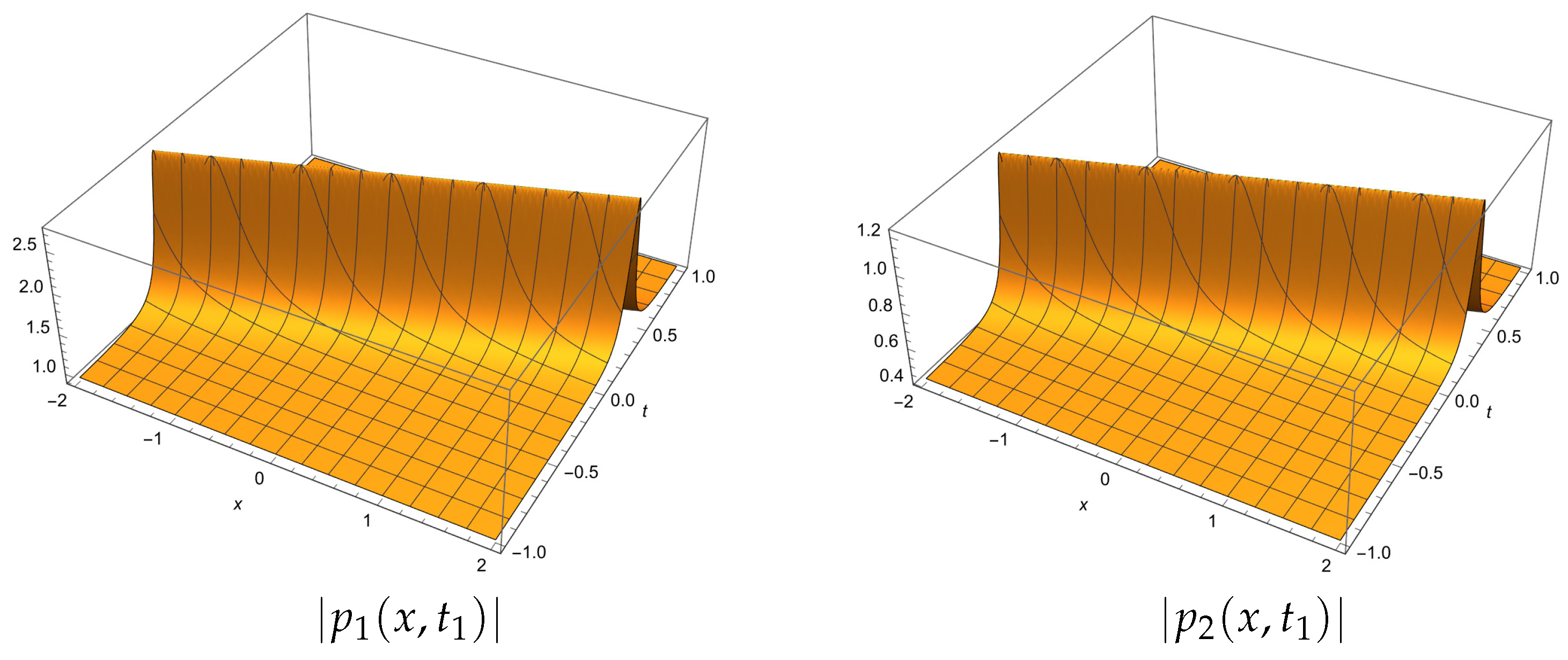
It is easy to see that when $3a^4>2m$ the solution (38) satisfies the reductions $q_j=-p_j^{*}$. The amplitudes of the solution components are depicted in Figure 1.

Figure 1. The amplitudes of the solution (38) for $a=1$, $m=1$.

The equation of the spectral curve for solution (38) takes the form

$$\begin{array}{c}\mathcal{R}(\mu ,\lambda )=\left(\mu -{\displaystyle \frac{1}{3}}{\lambda }^3-2a^2\lambda \right)\hfill \\ \hspace{1em}\hspace{1em}\hspace{1em}\hspace{1em}\hspace{1em}\hspace{1em}\hspace{1em}\times \left({\mu }^2+\left({\displaystyle \frac{1}{3}}{\lambda }^3+2a^2\lambda \right)-{\displaystyle \frac{2}{9}}{\lambda }^6-{\displaystyle \frac{8}{3}}{a}^2{\lambda }^4-11a^4{\lambda }^2-16a^6\right)=0.\hfill \end{array}$$

(39)

Note that since the solution components $p_1$ and $p_2$ are linearly dependent, the spectral curve splits into two. The first one is rational and is defined by the equation

$$\mu =\left({\displaystyle \frac{1}{3}}{\lambda }^2+2a^2\right)\lambda .$$

The equation for the second component of the curve is given by

$${\tilde{\mu }}^2={({\lambda }^2+4a^2)}^3,\mu ={\displaystyle \frac{1}{2}}\tilde{\mu }-{\displaystyle \frac{1}{6}}{\lambda }^3-a^2\lambda .$$

In other words, the second component of the curve (39) represents a degenerate hyperelliptic curve of genus $g=2$. The presence of branch points of the third order on the spectral curve corresponds to the existence of solutions in terms of rational functions.

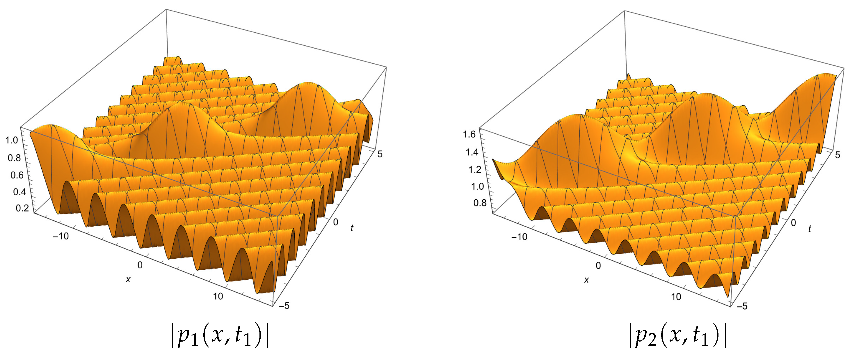
If the function $\widehat{v}$ is defined by Equation (37) and $\widehat{v}\ne const$, then

$$\begin{array}{cc}\hfill & u_1=-{\displaystyle \frac{(a^8+2a^6{b}^2-2a^{4}m-2a^2{b}^{2}m+b^{4}m)(2b^2+a^2(1+b^4{X}_1^2))}{2a^6(a^2+2b^2)(1+b^4{X}_1^2)}}\hfill \\ \hfill & +{\displaystyle \frac{b^5\sqrt{(4a^2-b^2)(a^8+2a^6{b}^2-4m^2)}{X}_1}{2a^5\sqrt{a^2+2b^2}(1+b^4{X}_1^2)}}cos\left(a\sqrt{a^2+2b^2}{X}_2\right)\hfill \\ \hfill & -{\displaystyle \frac{b^3\sqrt{(4a^2-b^2)(a^8+2a^6{b}^2-4m^2)}(2b^2+a^2(1-b^4{X}_1^2))}{4a^6(a^2+2b^2)(1+b^4{X}_1^2)}}\hfill \\ \hfill & \times sin\left(a\sqrt{a^2+2b^2}{X}_2\right),\hfill \\ \hfill & u_2=-{\displaystyle \frac{(a^8+2a^6{b}^2+2a^{4}m+2a^2{b}^{2}m-b^{4}m)(2b^2+a^2(1+b^4{X}_1^2))}{2a^6(a^2+2b^2)(1+b^4{X}_1^2)}}\hfill \\ \hfill & -{\displaystyle \frac{(b^5\sqrt{(4a^2-b^2)(a^8+2a^6{b}^2-4m^2)}{X}_1}{2a^5\sqrt{a^2+2b^2}(1+b^4{X}_1^2)}}cos\left(a\sqrt{a^2+2b^2}{X}_2\right)\hfill \\ \hfill & +{\displaystyle \frac{(b^3\sqrt{(4a^2-b^2)(a^8+2a^6{b}^2-4m^2)}(2b^2+a^2(1-b^4{X}_1^2))}{4a^6(a^2+2b^2)(1+b^4{X}_1^2)}}\hfill \\ \hfill & \times sin\left(a\sqrt{a^2+2b^2}{X}_2\right),\hfill \end{array}$$

where

$$X_1=x-(2a^2+b^2)t_1+X_{10},X_2=x-(3a^2+b^2)t_1+X_{20}.$$

Here, $X_{10}=X_1(0,0)$ and $X_{20}=X_2(0,0)$ are initial phases.

Equation (13) is two-phased and represents a nonlinear superposition of rational and trigonometric functions. In other words, the solution is a traveling rational wave on a trigonometric background. Expressions for the components $p_j$ and $q_j$ can be obtained from Equations (21) and (22). The amplitudes of the components of this solution are shown in Figure 2.

Figure 2. The amplitudes of the components of the traveling rational wave on a trigonometric background for $a=1$, $b=1$, $m=1/2$, $X_{10}=X_{20}=0$.

In this case, the equation of the spectral curve has the form given in (10), where

$$\begin{array}{cc}\hfill & \mathcal{A}\left(\lambda \right)=-{\displaystyle \frac{1}{3}}{\lambda }^6-{\displaystyle \frac{2(2a^2+b^2)}{3}}{\lambda }^4-{\displaystyle \frac{2a^4+2a^2{b}^2+5b^4}{6}}{\lambda }^2-{\displaystyle \frac{b^6}{4}},\hfill \\ \hfill & \mathcal{B}\left(\lambda \right)={\displaystyle \frac{2}{27}}{\lambda }^9+{\displaystyle \frac{2(2a^2+b^2)}{9}}{\lambda }^7+{\displaystyle \frac{10a^4+10a^2{b}^2+7b^4}{18}}{\lambda }^5\hfill \\ \hfill & +{\displaystyle \frac{35b^6+48a^2{b}^4-12a^4{b}^2-8a^6}{108}}{\lambda }^3+{\displaystyle \frac{7b^8-4a^2{b}^6}{48}}\lambda .\hfill \end{array}$$

(40)

The discriminant of the polynomial $\mathcal{R}\left(\mu \right)$ with coefficients given by (40) is equal to

$$\mathcal{D}\left(\lambda \right)={\displaystyle \frac{1}{256}}{(4a^2{\lambda }^2+b^4)}^3(4(a^2+2b^2){\lambda }^4+(16a^4+40a^2{b}^2+13b^4){\lambda }^2+16b^6).$$

Therefore, the spectral curve (10), (40) is degenerate. It has two branch points of the third order and four branch points of the first order. The presence of branch points of the third order indicates a dependence of the solution on rational functions.

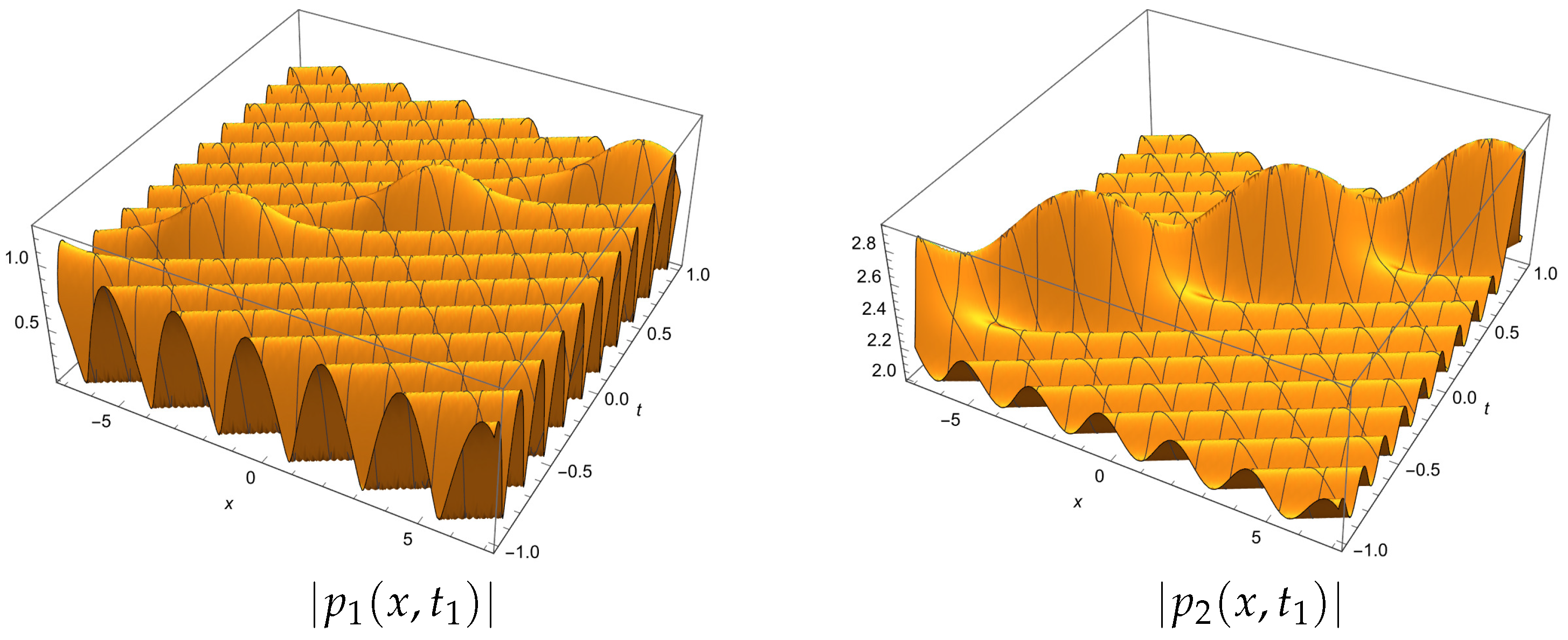
5.3. Case of the Function $u\left(x\right)$ in the Form of a Soliton

Let

$$u=-b^2-a\mathrm{sech}\left(a{X}_1\right)<0,$$

(41)

where $X_1=x-c_2{t}_1$. Then,

$$c_2=2b^2,c_{5,6}={\displaystyle \frac{a^2-2b^4}{4}}\pm m,c_7=(a^2-b^4)b^4,{\mathcal{A}}_3=0,$$

where $a>0$, $b>0$, $m>0$.

With these values of constants, Equation (29) takes the form

$${\left({\partial }_{x}u\right)}^2=-{(u+b^2)}^2(u^2+2b^{2}u+b^4-a^2).$$

Since

$$\begin{array}{cc}\hfill & {\kappa }^2-{(c_5+c_6)}^2=-{\displaystyle \frac{1}{4}}{a}^4<0,\hfill \\ \hfill & {\kappa }^2-{(c_5-c_6)}^2=b^4(b^4-a^2)-4m^2,\hfill \end{array}$$

Then, the solution will be real when $4m^2>b^4(b^4-a^2)$. In other words, Function (41) corresponds to the inequality $|\widehat{v}| > 1$.

In this case, Equation (30) can be written in the following form:

$$\int {\displaystyle \frac{d\widehat{v}}{\sqrt{-a^4-16m^2+8(a^2-2b^4)m\widehat{v}+4b^4(a^2-b^4){\widehat{v}}^2}}}={\displaystyle \frac{1}{2}}\int {\displaystyle \frac{dx}{b^2+a\mathrm{sech}\left(ax\right)}}.$$

Both integrals in this equality depend on the relationship between a and $b^2$.

Let $a<b^2$ and $2m>b^2\sqrt{b^4-a^2}$. Then the solution of Equation (30) has the form

$$\begin{array}{c}\widehat{v}={\displaystyle \frac{(2b^4-a^2)m}{b^8-a^2{b}^4}}+{\displaystyle \frac{a^2\sqrt{4m^2-b^8+a^2{b}^4}}{2(b^8-a^2{b}^4)}}\hfill \\ \hspace{1em}\hspace{1em}\hspace{1em}\hspace{1em}\hspace{1em}\hspace{1em}\hspace{1em}\hspace{1em}\times \left({\displaystyle \frac{b^2+acosh\left(a{X}_1\right)}{a+b^{2}cosh\left(a{X}_1\right)}}sin\left(\sqrt{b^4-a^2}{X}_2\right)\right.\hfill \\ \hspace{1em}\hspace{1em}\hspace{1em}\hspace{1em}\hspace{1em}\hspace{1em}\hspace{1em}\hspace{1em}\hspace{1em}\hspace{1em}\hspace{1em}\left.+{\displaystyle \frac{(a^2-b^4)sinh\left(a{X}_1\right)}{\sqrt{b^4-a^2}(a+b^{2}cosh\left(a{X}_1\right)}}cos\left(\sqrt{b^4-a^2}{X}_2\right)\right).\hfill \end{array}$$

(42)

From Equations (2) and (42), it follows that

$$\begin{array}{cc}\hfill & u_1=-{\displaystyle \frac{(-a^2{b}^4+b^8+a^{2}m-2b^{4}m)(b^2+a\mathrm{sech}\left(a{X}_1\right))}{2b^4(b^2-a)(a+b^2)}}\hfill \\ \hfill & -{\displaystyle \frac{a^2\sqrt{a^2{b}^4-b^8+4m^2}(b^2\mathrm{sech}\left(a{X}_1\right)+a)sin\left(\sqrt{b^4-a^2}{X}_2\right)}{4b^4(b^2-a)(a+b^2)}}\hfill \\ \hfill & +{\displaystyle \frac{a^2\sqrt{a^2{b}^4-b^8+4m^2}tanh\left(a{X}_1\right)cos\left(\sqrt{b^4-a^2}{X}_2\right)}{4b^4\sqrt{b^4-a^2}}},\hfill \\ \hfill & u_2=-{\displaystyle \frac{(-a^2{b}^4+b^8-a^{2}m+2b^{4}m)(b^2+a\mathrm{sech}\left(a{X}_1\right))}{2b^4(b^2-a)(a+b^2)}}\hfill \\ \hfill & +{\displaystyle \frac{a^2\sqrt{a^2{b}^4-b^8+4m^2}(b^2\mathrm{sech}\left(a{X}_1\right)+a)sin\left(\sqrt{b^4-a^2}{X}_2\right)}{4b^4(b^2-a)(a+b^2)}}\hfill \\ \hfill & -{\displaystyle \frac{a^2\sqrt{a^2{b}^4-b^8+4m^2}tanh\left(a{X}_1\right)cos\left(\sqrt{b^4-a^2}{X}_2\right)}{4b^4\sqrt{b^4-a^2}}},\hfill \end{array}$$

where $X_1=x-2b^2{t}_1+X_{10}$, $X_2=x-3b^2{t}_1+X_{20}$. The amplitudes of the components of this solution are shown in Figure 3.

Figure 3. The amplitudes of the solitonic solution for $a=3$, $b=2$, $m=6$, $X_{10}=X_{20}=0$.

In this case, the equation of the spectral curve has the form (10), where

$$\begin{array}{cc}\hfill & \mathcal{A}\left(\lambda \right)=-{\displaystyle \frac{1}{3}}{\lambda }^6-{\displaystyle \frac{4b^2}{3}}{\lambda }^4-{\displaystyle \frac{3a^2+2b^4}{6}}{\lambda }^2,\hfill \\ \hfill & \mathcal{B}\left(\lambda \right)={\displaystyle \frac{2}{27}}{\lambda }^9+{\displaystyle \frac{4b^2}{9}}{\lambda }^7+{\displaystyle \frac{3a^2+10b^4}{18}}{\lambda }^5+{\displaystyle \frac{b^2(9a^2-2b^4)}{27}}{\lambda }^3+{\displaystyle \frac{a^4}{16}}\lambda .\hfill \end{array}$$

(43)

The discriminant of the polynomial $\mathcal{R}\left(\mu \right)$ with coefficients (43) is equal to

$$\mathcal{D}\left(\lambda \right)={\displaystyle \frac{1}{256}}{\lambda }^2{(4b^2{\lambda }^2+a^2)}^2(16(b^4-a^2){\lambda }^4+(64b^6-72a^2{b}^2){\lambda }^2-27a^4).$$

Therefore, the spectral curve (10), (43) is degenerate. It has three branch points of the second order and four branch points of the first order.

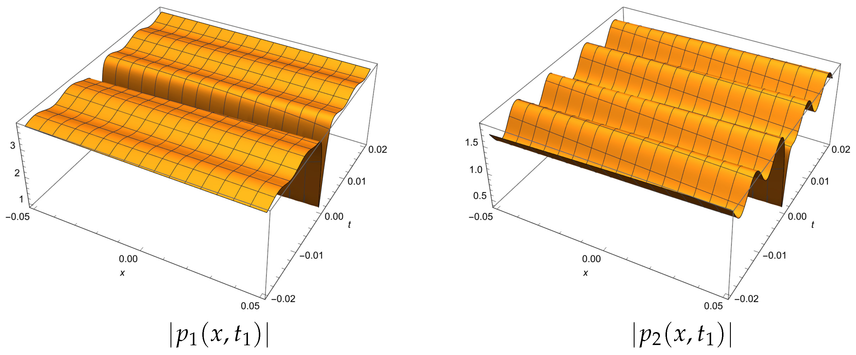
5.4. Case of the Function $u\left(x\right)$ in the Form of a Dark Soliton

Let

$$u={\displaystyle \frac{2a{b}^2(1+b^2)}{{tanh}^2\left(ab{X}_1\right)+b^2}}-k^2<0$$

(44)

where $X_1=x-c_2{t}_1+X_{10}$. Then,

$$\begin{array}{c}{c}_2=2k^2-a(1+3b^2),c_{5,6}={\displaystyle \frac{1}{4}}\left((1-2b^2-3b^4)a^2+(1+3b^2)a{k}^2-2k^4\right)\pm m,\\ c_7=(2a(1+b^2)-k^2){(k^3-2a{b}^{2}k)}^2,{\mathcal{A}}_3=-{\displaystyle \frac{1}{4}}{a}^3(b^2-1){(b^2+1)}^2,\end{array}$$

where $a>0$, $b>0$, $m>0$, $k>0$. With these values of constants, Equation (29) takes the form

$${\left({\partial }_{x}u\right)}^2=-(u+k^2)(u+k^2-2a(1+b^2)){(u+k^2-2a{b}^2)}^2.$$

Since

$$\begin{array}{cc}\hfill & {\kappa }^2-{(c_5+c_6)}^2={\displaystyle \frac{1}{4}}{a}^3{(b^2+1)}^2(4(b^2-1)k^2-a{(1-3b^2)}^2),\hfill \\ \hfill & {\kappa }^2-{(c_5-c_6)}^2=(k^2-2a(1+b^2)){(k^3-2a{b}^{2}k)}^2-4m^2,\hfill \end{array}$$

Therefore, the inequality $|\widehat{v}| < 1$ is true under the following conditions:

$$\begin{array}{cc}\hfill & b>1,k^2>{\displaystyle \frac{a{(1-3b^2)}^2}{4(b^2-1)}},\hfill \\ \hfill & k^2>2a(1+b^2),4m^2<(k^2-2a(1+b^2)){(k^3-2a{b}^{2}k)}^2.\hfill \end{array}$$

With these parameter values, Equality (30) takes the form

$$\begin{array}{c}\widehat{v}={\displaystyle \frac{a^{3/2}(b^2+1)\sqrt{4(b^2-1)k^2-a{(1-3b^2)}^2}}{2(k^2-2a(1+b^2)){(k^3-2a{b}^{2}k)}^2}}\hfill \\ \hspace{1em}\hspace{1em}\hspace{1em}\hspace{1em}\hspace{1em}\hspace{1em}\hspace{1em}\times \sqrt{(k^2-2a(1+b^2)){(k^3-2a{b}^{2}k)}^2-4m^2}sin\left(\kappa \theta \right)\hfill \\ \hspace{1em}\hspace{1em}\hspace{1em}\hspace{1em}\hspace{1em}\hspace{1em}\hspace{1em}\hspace{1em}\hspace{1em}\hspace{1em}\hspace{1em}\hspace{1em}\hspace{1em}\hspace{1em}-{\displaystyle \frac{(a^2(-1+2b^2+3b^4)-2a(1+3b^2)k^2+2k^4)m}{(k^2-2a(1+b^2)){(k^3-2a{b}^{2}k)}^2}}\hfill \end{array}$$

where

$$\kappa \theta =2arctan\left({\displaystyle \frac{ktanh\left(ab{X}_1\right)}{b\sqrt{k^2-2a(b^2+1)}}}\right)+k\sqrt{k^2-2a(b^2+1)}\left(X_1-(k^2-2a{b}^2)t_1\right).$$

Using trigonometric identities, we obtain the following relation:

$$\begin{array}{c}sin\left(\kappa \theta \right)={\displaystyle \frac{2bk\sqrt{k^2-2a(b^2+1)}tanh\left(ab{X}_1\right)}{(k^2-2a(b^2+1))b^2+k^2{tanh}^2\left(ab{X}_1\right)}}cos\left(X_2\right)\hfill \\ \hspace{1em}\hspace{1em}\hspace{1em}\hspace{1em}\hspace{1em}\hspace{1em}\hspace{1em}\hspace{1em}\hspace{1em}\hspace{1em}\hspace{1em}\hspace{1em}\hspace{1em}\hspace{1em}\hspace{1em}+{\displaystyle \frac{(k^2-2a(b^2+1))b^2-k^2{tanh}^2\left(ab{X}_1\right)}{(k^2-2a(b^2+1))b^2+k^2{tanh}^2\left(ab{X}_1\right)}}sin\left(X_2\right),\hfill \end{array}$$

where

$$X_2=k\sqrt{k^2-2a(b^2+1)}(x-(3k^2-a(1+5b^2))t_1)+X_{20}.$$

In Figure 4, the amplitudes of the solution components are depicted, where the length of the solution is equal to $\left|\mathbf{p}\right|=\sqrt{-u}$, and u is determined by Equation (44).

Figure 4. The amplitudes of the dark solitonic solution for $a=8$, $b=2$, $k=9$, $m=76$, $X_{10}=X_{20}=0$.

The coefficients of the equation of the spectral curve (10) in this case are

$$\begin{array}{cc}\hfill & \mathcal{A}\left(\lambda \right)=-{\displaystyle \frac{1}{3}}{\lambda }^6+{\displaystyle \frac{2}{3}}(a(1+3b^2)-2k^2){\lambda }^4\hfill \\ \hfill & -{\displaystyle \frac{1}{6}}(a^2(5+6b^2+9b^4)-2a(1+1b^2)k^2+2k^4){\lambda }^2-{\displaystyle \frac{1}{4}}{a}^3(b^2-1){(b^2+1)}^2,\hfill \\ \hfill & \mathcal{B}\left(\lambda \right)={\displaystyle \frac{2}{27}}{\lambda }^9-{\displaystyle \frac{2}{9}}(a(1+3b^2)-2k^2){\lambda }^7\hfill \\ \hfill & +{\displaystyle \frac{1}{18}}(a^2(7+18b^2+27b^4)-10a(1+3b^2)k^2+10k^4){\lambda }^5\hfill \\ \hfill & -{\displaystyle \frac{1}{108}}(a^3(35+99b^2+45b^4+45b^6)-48a^2{k}^2-12a(1+3b^2)k^4+8k^6){\lambda }^3\hfill \\ \hfill & +{\displaystyle \frac{1}{48}}{a}^3{(1+b^2)}^2(a(7-10b^2+15b^4)-4(-1+b^2)k^2)\lambda .\hfill \end{array}$$

The discriminant of the polynomial $\mathcal{R}\left(\mu \right)$ with these coefficients is

$$\begin{array}{c}\mathcal{D}\left(\lambda \right)={\displaystyle \frac{1}{256}}{\left(a^2{(1+b^2)}^2+4(k^2-2a{b}^2){\lambda }^2\right)}^2(6a^5{(-1+b^2)}^3{(1+b^2)}^2\\ +a^2(-a^2{(1+b^2)}^2(-13-10b^2+131b^4)+8a(-13-5b^2+13b^4+5b^6)k^2\\ +16{(-1+b^2)}^2{k}^4){\lambda }^2+8(a^3{(1+b^2)}^2(-1+3b^2)+a^2(7+30b^2+23b^4)k^2\\ -4a(5+7b^2)k^4+8k^6){\lambda }^4+16k^2(-2a(1+b^2)+k^2){\lambda }^6).\end{array}$$

Therefore, in this case, the spectral curve is also degenerate. It has two complex conjugate branch points of the second order and three pairs of complex conjugate branch points of the first order.

6. Concluding Remarks

The investigation of simple nontrivial solutions of the vector Gerdjikov–Ivanov equation has revealed the following properties:

• This equation is invariant under orthogonal transformations of solutions. The spectral curves of multiphase solutions are also invariant under orthogonal transformations of solutions. In other words, the direction of the wave vector cannot be determined from the spectral curve.
• The procedure for constructing simple nontrivial solutions of these equations has shown that an equation for the length of the vector appears first. Then, from additional relations, an equation determining the dependence of the vector’s direction on its length follows. Thus, the solution of the equation is determined not so much by the dynamics of its components as by the dynamics of the vector’s length and direction.
• For all vector equations, there are parameter values for which the direction of the vector is fixed. In these cases, the spectral curve breaks down into separate components, and the evolution of the vector is determined by a curve of a lower genus than in the case when the vector’s direction is not fixed.

Therefore, it is necessary to take into account the presence of these symmetries when reconstructing a signal from its spectral data.