Modelling a Market Society with Stochastically Varying Money Exchange Frequencies

Abstract

We propose and examine a model expressed by stochastic differential equations for the evolution of a complex system. We refer in particular to a market society, in which the state of each individual is identified by the amount of money at his/her disposal. The evolution of such a system over time is described by suitable equations that link the instantaneous changes in the probability of each state with the probable outcomes of pairwise interactions between elements of the system. In the context at hand, these pairwise interactions simply represent money exchanges, due to the sales and purchases of goods and services. In this paper, unlike the usual method in the literature, the interaction frequencies and the consequent probabilities of passing from one state to another are not considered as assigned once and for all but are supposed to be randomly variable. This choice, as also shown by several numerical simulations, seems likely to have fruitful consequences, especially for a more realistic representation of economic issues and phenomena.

1. Introduction

The purpose of the present work is to further develop the analysis carried out in [1], which considered a description in the framework of kinetic theory of the evolution of an economic system, or, more precisely, a market system. We mean by this a system of mutually interacting individuals—who could be called “economic agents”—whose states are characterized by the amount of money at their disposal and whose mutual interactions are simply money exchanges that occur due to the sales and purchases of goods and/or services. As is well known, in a statistical framework, the changes in state due to interactions between economic agents cannot be deterministically predicted: all that can be accomplished is to attribute a probability linked to the state before the interaction to each possible state after the interaction. This is what is called “transition probability”, and this probability also depends on the state of the subject interacting with an individual. Usually, the law that associates to any triple $(s,s^{\prime },s^{″})$ of states, the probability that any individual goes from state s to $s^{\prime }$ after an interaction with an economic agent whose state is $s^{″}$ is assigned more or less arbitrarily, according to a statistical projection from a sufficiently large number of previous experiences. And, of course, the instantaneous variation of the probability of each state also depends on the interaction rate, which, in an economic context, is the frequency of money exchanges per unit time. Thus, this variation is a function of two sets of terms: (1) the “assigned” terms, which are independent of the evolution of the system (interaction rates and probability transitions), and (2) the unknown terms, which are the states of interacting individuals before the interaction.

The assigned terms that determine the variation in the probability distribution over the set of states are usually considered as characterizing the particular system under examination. Accordingly, they are prescribed once and for all on the basis of a sufficiently large number of prior experiments. The correctness of the prescription is checked based on the greater or lesser agreement of the solutions to the equations with the observed evolution of the system. In this connection, a question spontaneously arises: can we improve this procedure by taking into account a priori any possibility of error in the prescription or uncertainty? The main purpose of this paper is to give this question an affirmative answer. As a matter of fact, if the interaction frequencies and transition probabilities, rather than constants uniquely associated with the model, are assumed to be “random variables” or, more precisely, values affected by randomly distributed errors, one obtains at least two important results: $\left(1\right)$ on the one hand, as we shall see in details in Section 2 and Section 3, one finds convincing evidence of the validity of the continuous dependence of solutions on the data (where the word “data” also refers to coefficients, when these latter are interpreted as parameters); $\left(2\right)$ on the other hand, with particular regard to the economic context, it allows us to outline an explanation of the fluctuations that affect the overall economic state of a collectivity. These results will be illustrated in this paper through the outputs of some numerical simulations, in which the errors and uncertainties are assumed to be distributed according to the standard normal distribution and the extraction of their random values is performed at each time step.

To put the article in context, we point out that, especially over the last fifteen years or so, several works have been published studying markets and economic exchanges from a kinetic theory perspective. To mention just a few of these works, without any claim to completeness, we recall here [2,3,4,5,6], referring to their bibliographies as well. It is worthwhile to stress that, despite the common basis that rests on the analogy between individuals exchanging money and molecules undergoing collisions, these papers and those they quote in fact have developed different approaches. In particular, their approaches and methods are significantly different from those presented here. Very briefly, in [2], various “gas-like” models are reviewed, which rely on a simple framework in which two (out of N) randomly selected agents exchange money according to a predefined rule. Specific focus is placed on the effect of different saving propensity attitudes of the traders on the resulting long-time wealth distribution. In [4], similar asset exchange models are considered in conjunction with a utility maximization principle for the pairs of trading agents. Monte Carlo simulation methods are then employed to analyze the distributional features. The approach in [3] differs from those just mentioned, because it treats the agents as a continuum and defines the dynamics as governed by a spatially homogeneous Boltzmann equation in which the term containing the “collisional operator” (in this context, collisions correspond to trades) is expressed by an integral. In this paper, the analysis focuses on the thickness of the Pareto tail. An analog of the Boltzmann equation is also considered in [6], which leads, in a suitable (small transaction) limiting case, to a partial integrodifferential equation. Features such as inflation, production, and taxation are also added to the model. Finally, the survey [5] provides an extensive description of the historical development of several statistical models of money, wealth, and income distributions, and includes in this overview both gas-like models that involve N agents and models described by integrodifferential equations.

Unlike ours, none of the mentioned papers take into account the distinction of different income classes. Furthermore, the uncertainty that affects the encounter rates and is incorporated into the present work by means of random variables, has (to the best of our knowledge) never been dealt with as here. Regarding this aspect of stochasticity, a final caveat is also necessary. The explicit incorporation of a noise term in a model of the dynamics of income distribution in the presence of monetary exchanges was the subject of the article [7] and resulted in a Langevin-type kinetic equation somehow similar to the one below. We emphasize, however, that the type of noise and uncertainty, as well as the aims pursued in the investigation, are very different in [7] and here. Whereas in [7], a term expressing a multiplicative noise, unrelated to interaction rates, is added to the deterministic part of the evolution equation, in the present paper it is the coefficients themselves that express the interaction probabilities between individuals that are considered randomly changing over time.

We underline that the stochastic frame formulated in this paper should essentially be understood as a basis building block for future investigations in which we plan to address specific topics of economic interest in a more targeted way. Additionally, we think and hope that it can be a stimulus for in-depth analytical studies and for the establishment of well-posedness results. Indeed, we do not provide here formal proofs of the global existence and uniqueness of solutions of the proposed nonlinear stochastic differential equations. Rather, we pursue a heuristic approach by developing and discussing numerical simulations. We emphasize, however, that all the numerical simulations we have carried out (actually, a large number; those reported here are only a sample) suggest that the proposed model is reasonable and deserves attention and further investigation.

The contents of the paper are distributed as follows: Section 2 is devoted to the statement of the problem, to the explanation of the mathematical language used to treat it, and to the formulation of the system of stochastic equations describing the evolution of an economic system under our hypotheses; in Section 3, we comment on simulations and show a sample of numerical solutions to the system considered in Section 2, also discussing their connection with the problem of the continuous dependence of solutions on parameters. Section 4 is devoted to outlining some conclusions and possible developments of the present research towards the construction of models that are increasingly faithful to the behavior of real economic societies. Finally, an appendix (Appendix A) is added containing the proof of the fact that a certain quantity is conserved during the evolution of the system.

2. The Model

We consider here a closed market society, characterized by the fact that the frequencies with which the individuals exchange money vary stochastically over time. We describe the problem in the context of a complex system approach, considering a population of interacting individuals divided into a finite number n of classes characterized by the average income of their members. To fix the notations, we first take $n+1$ numbers $0={\rho }_0<{\rho }_1<...<{\rho }_n$, where ${\rho }_n$ is large enough to represent an upper bound for the maximal conceivable income of each individual in the society. In particular, we suppose that ${\rho }_{i+1}-{\rho }_i=\alpha ({\rho }_i-{\rho }_{i-1})$ with $\alpha >1$, for $i=1,...,n-1$. Consequently, one can consider n intervals $[{\rho }_{i-1},{\rho }_i)$ of increasing length, identifying n income classes. Even if n is not very large, we can obtain, by suitably choosing $\alpha$, that the income of individuals belonging to the n-th class is orders of magnitude larger than that of the individuals of the first class (as happens in real societies). We denote by $r_i=({\rho }_i+{\rho }_{i-1})/2$ for $i=1,...,n$ the average income of the i-th class and, assuming for simplicity that all individuals with income $\rho \in [{\rho }_{i-1},{\rho }_i)$ actually have the same average income $r_i$, we denote by $x_i=x_i\left(t\right)$ for $i=1,...,n$ the “fraction” (portion) of these individuals at time t.

Our aim is to study the variation over time of the number of individuals belonging to each class, due to the whole of economic exchanges that take place between the individuals themselves.

We deal with a case in which the global income is constant. Namely, we assume that only many transfers of money from one individual to another occur. The elementary model of society we have in mind is one in which payments from one individual to another are motivated by the provision of a service, good or job. The effect of these economic transfers is that of a continuous displacement of individuals from one class to another. Of course, in correspondence with a single transaction, this displacement is “small”: we can interpret it as the displacement of portions of individuals, an interpretation that is justified in the context of a collective picture. At the “macroscopic level”, the conservation of global income can be interpreted as the fact that production and consumption in the society are balanced.

To set up a mathematical formulation of the economic exchanges process described, we introduce n matrices $C^i$ with $i=1,...,n$, of dimension $n\times n$, with the following property: the elements $c_{hk}^i$ of $C^i$ satisfy $c_{hk}^i\in [0,1]$ and $c_{hk}^i$ expresses the probability that an individual of the h-th class belongs to the i-th class after a direct interaction with an individual of the k-th class. Of course, the requirement that the coefficients $c_{hk}^i$ express probabilities implies that for any fixed h and k they satisfy ${\displaystyle \sum _{i=1}^n{c}_{hk}^i=1}$.

A suitable expression for these coefficients has been derived in [1] (note only that in [1] the case of income intervals of the same length was considered, i.e., the case where $\alpha =1$). To reproduce and then adapt it to the new framework, we introduce an $n\times n$ matrix P, whose elements $p_{h,k}$ for $h,k=1,...,n$ denote the probability that, in an encounter between an individual of the h-th class and one of the k-th class, the one who pays is the former (also called a h-individual). We denote by S the amount paid in a transaction. As mentioned above, any single interaction may cause a slight decrease or increase in the income of the individuals involved and, in turn, a slight variation in the class populations. In fact, these variations only affect the original class and the neighboring classes of the individuals involved, and the only possibly nonzero elements among the $c_{hk}^i$ are easily found (see [1] for these details) to take the form

$$c_{h,k}^i=a_{h,k}^i+b_{h,k}^i,$$

(1)

where the only nonzero elements $a_{h,k}^i$—elements of n matrices $A^i$—are

$$a_{i,k}^i=1,\mathrm{for}i,k=1,...,n,$$

(2)

whereas the nonzero elements $b_{h,k}^i$—elements of n matrices $B^i$—are given by

$$\begin{array}{ccc}\hfill b_{i+1,k}^i& =& p_{i+1,k}\frac{S}{r_{i+1}-r_i},\hfill \\ \hfill b_{i,k}^i& =& -p_{k,i}\frac{S}{r_{i+1}-r_i}-p_{i,k}\frac{S}{r_i-r_{i-1}},\hfill \\ \hfill b_{i-1,k}^i& =& p_{k,i-1}\frac{S}{r_i-r_{i-1}}.\hfill \end{array}$$

(3)

Note that the expression for $b_{i+1,k}^i$ in (3) holds true for $i\le n-1$ and $k\le n-1$, the first addendum of the expression for $b_{i,k}^i$ is actually only present for $i\le n-1$ and $k\ge 2$, while the second addendum is present only under the condition that $i\ge 2$ and $k\le n-1$; and the expression for $b_{i-1,k}^i$ holds true for $i\ge 2$ and $k\ge 2$. These constraints are functional to the meaningfulness of the indices and reflect the fact that in this model individuals of the first class never pay and individuals of the n-th class never receive money (there are neither classes poorer than the first nor classes richer than the n-th).

There is an element of symmetry in the Formula (3) since in each trade the variation in the fraction of i-individuals for $2\le i\le n-1$, regardless of whether they pay an individual of a poorer or richer class, is inversely proportional to the difference in the average incomes of the classes involved in the exchange. Perfect symmetry, however, cannot be achieved in this case, because the average income $r_i$ of the i-th class increases as i increases.

We emphasize that there are some degrees of freedom in the choice of the coefficients $p_{h,k}$. It is reasonable, in this respect, to adjust the coefficients based on the fact that poorer individuals usually earn and spend less than richer ones. An even more realistic option is to also take into account the effects of some unavoidable uncertainties and randomness. In view of this, we consider each $p_{h,k}$ for $h,k=1,...,n$ as the sum of a “deterministic” and a “stochastic” part,

$$p_{h,k}=p_{h,k}^d+p_{h,k}^s,$$

(4)

or, in matrix notation,

$$P=P^d+P^s.$$

To this aim, we start by defining a $n\times n$ matrix

$$Q=Q(c,M)=\left\{q_{h,k}\right\},$$

where the variable c is a positive number and the variable $M=\left\{M_{h,k}\right\}$ is a $n\times n$ matrix, as the matrix with elements $q_{h,k}$ given by

$$\begin{array}{ccc}\hfill q_{h,k}& =& c{M}_{h,k}\frac{min\{r_h,r_k\}}{r_n}\mathrm{for}h=2,...,n\mathrm{and}k=1,...,n-1,\hfill \\ \hfill q_{1,k}& =& 0\mathrm{for}k=1,...,n,\hfill \\ \hfill q_{h,n}& =& 0\mathrm{for}h=1,...,n.\hfill \end{array}$$

(5)

We then define

$$P^d=Q(c_d,M^1),$$

and

$$P^s=P^s\left(dW\right)=Q(c_s,dW),$$

(with the dependence of $P^s$ on $dW$ explicitly underlined) where $M^1$ is the $n\times n$ matrix having all elements equal to 1, W is a $n\times n$ matrix whose elements are Brownian motions and $c_d$ and $c_s$ are positive constants, chosen in such a way that the inequalities

$$0\le p_{h,k}\le 1\mathrm{and}{p}_{h,k}+p_{k,h}\le 1$$

(6)

hold for all $h,k=1,...,n$ with a probability very close to 1. In particular, in Section 3, a numerical approximation is proposed, according to which the (6) are satisfied; and this in turn guarantees that the $x_i$ remain non-negative during the evolution of the system. These latter conditions are compatible with the meaning of the $p_{h,k}$, which express the probabilities of payment in a case in which encounters without any payment can also occur.

The overall dynamics corresponding to the variation of the fraction of individuals in the various income classes is described by a vectorial stochastic differential equation (see, e.g., [8,9,10] for SDE, [11] for a nice presentation of SDE and their numerical treatment and [12]). Before writing it down, let us point out that in the following we denote $B^i\left(P^d\right)$ (respectively, $B^i\left(P^s\left(dW\right)\right)$) the matrix $B^i$ having elements $b_{h,k}^i$ as in the Formula (3), with the difference, however, that the elements $p_{h,k}$ are replaced by $p_{h,k}^d$ (respectively, $p_{h,k}^s$).

The announced stochastic differential equation, whose unknown is the vector function $x=(x_1,x_2,...,x_n)$ with components $x_i$ denoting the number of individuals in the i-th income class for $i=1,...,n$, is given by

$$\begin{array}{ccc}\hfill d{x}_i& =& \left(\sum _{h,k=1}^n\left(a_{hk}^i+b_{hk}^i\left(P^d\right)\right)x_h{x}_k-\sum _{h,k=1}^n\left(a_{ik}^h+b_{ik}^h\left(P^d\right)\right)x_i{x}_k\right)dt\hfill \\ & +& \sum _{h,k=1}^n{b}_{hk}^i\left(P^s\left(dW\right)\right)x_h{x}_k,\mathrm{for}i=1,...,n.\hfill \end{array}$$

(7)

By taking the sum over $i=1,...,n$ of the left(-hand) and of the right(-hand) side of (7), one can easily see that (the size of) the total population, ${\displaystyle \sum _{i=1}^n}{x}_i\left(t\right)$, remains constant in time. This is in agreement with the fact that births, deaths and other variations in the total number of individuals are not significant for the problem under investigation and over the period of interest here.

By choosing the normalization

$$\sum _{i=1}^n{x}_i\left(t\right)=1,$$

(8)

we observe that, since (as can easily be verified)

$$\sum _{h=1}^n\left(a_{ik}^h+b_{ik}^h\left(P^d\right)\right)=1,$$

one has

$$\sum _{h,k=1}^n\left(a_{ik}^h+b_{ik}^h\left(P^d\right)\right)x_i{x}_k=x_i\sum _{k=1}^n{x}_k=x_i.$$

(9)

The differential Equation (7) can then be written in a more compact and elegant form as

$$d{x}_i=\left(\right((A^i+B^i(P^d))x)·x-x_i)dt+\left(B^i\left(P^s\left(dW\right)\right)x\right)·x,\mathrm{for}i=1,...,n,$$

(10)

and in the numerical simulations we employ the usual approximation ([10,11,12])

$$\Delta x_i=\left(\right((A^i+B^i(P^d))x)·x-x_i)\Delta t+\left(B^i\left(P^s\left(X\right)\right)x\right)·x\sqrt{\Delta t},\mathrm{for}i=1,...,n,$$

(11)

where $X=\left\{X_{h,k}\right\}$ is a $n\times n$ matrix, whose elements are independent standard normal random variables. We emphasize that the extraction of the random variables $X_{h,k}$ occurs at each time step during the evolution of the system. Furthermore, we stress that the elements of the matrices $B^i$ depend linearly on the elements of the matrices $P^s$ and, in turn, these depend linearly on the elements of the matrices X. Yet, the Equation (10) is nonlinear.

In conclusion, the system of equations described above reflects the classical philosophy underlying the kinetic-theoretical treatment of the behavior of many-particles systems, but with one very important difference. The total probability variation of each possible state of the “particles” in the system results from the sum of a gain term and a loss term; but in the standard model, these are—in an appropriate sense of the term—deterministic: once the transition probabilities and interaction rates have been assigned, the time derivative of the probability of each state and the probability itself become—provided the equation can be solved—known functions of time. This is a peculiar feature of probability: although the events to which it applies are uncertain by definition, within the framework of a given theory, its values are certain. Accordingly, the interaction rates and the transition probabilities that appear in all kinetic-theoretical equations are in a sense the weak point of all models that use them. In any case, these parameters cannot be assigned exactly a priori or “by nose” if the models are to be applied to real problems. At most, their values can be proposed as working hypotheses and must be verified a posteriori.

The difference introduced in this paper lies in the additional term in the right-hand side of Equation (11). Containing a random variable distributed according to the standard Gauss normal curve of errors, this term takes into account the unavoidable uncertainty of the interactions rates and the parameters, or data, of the theory. The rigidity of precise assumptions about the prescription of conditional probabilities is mitigated and, as will be shown in Section 3 through a series of simulations, this approach can offer a broader class of solutions that exhibit more natural fluctuating behavior.

3. Numerical Results

Before moving to a discussion on the results of the numerical simulations, we point out that the specific structure of the coefficients (3) guarantees that the total income $\mathcal{I}\left(x\right)={\sum }_{j=1}^n{r}_j{x}_j\left(t\right)$ remains constant during the time evolution of the system described by both Equations (10) and (11). We refer the proof of this to the Appendix and we continue with the presentation here.

To investigate the processes generated by Equation (11), we have to fix some of the parameters of the model. As an example, we chose $n=9$ (but then, as also mentioned below, we also dealt with the cases $n=11$ and $n=13$) and $\alpha =1.35$. The values of the ${\rho }_j$ for $j=0,1,2,...,n$ were assumed to be approximately equal to

$$0,3.779,8.880,15.767,25.064,37.614,54.558,77.432,108.312,150,$$

with average incomes $r_j$ for $j=1,2,...,n$ approximately equal to

$$1.889,6.329,12.323,20.415,31.339,46.086,65.995,92.872,129.156.$$

The logic is to have the average income of the richest class two orders of magnitude larger than that of the poorest class. Also, we chose $S=3$. As for the parameters $p_{h,k}$ defined in (5), we chose $c_d=1/4$ and $c_s=1/12$, whereas for any h and any k in $\{1,2,...,n\}$ a (different) value $X_{h,k}$ of the standard normal random variable was taken at each time step. To be precise, in order to guarantee the validity of the inequalities (6), we took a truncated version of the standard normal random variable, restricting the values domain to the interval $[-3,3]$ (which contains, by the way, approximately $99\%$ of all possible values).

At this point, the following observation is in order: a quantity of simulations for the construction of numerical solutions of the “deterministic” problem, namely the problem described by Equation (11) in which $c_s=0$, gives evidence of the fact that—once the parameters n, $\alpha$, ${\rho }_j$ for $j=0,1,2,...,n$ and $r_j$ for $j=1,2,...,n$, S and $c_d$ are fixed—all solutions evolving from initial data $x\left(0\right)=x_0=(x_{01},\dots ,x_{0n})$ with $x_{0i}\ge 0$ for any $i=1,2,...,n$, which satisfy ${\sum }_{i=0}^n{x}_{0i}=1$ and ${\sum }_{i=1}^n{r}_i{x}_{0i}=\mu$ for some $\mu >0$, tend to the same stationary solution as $t\to \infty$ (actually, as t becomes large). In other words, when the parameters defining the “deterministic” model are fixed, in correspondence to any conceivable value $\mu$ of the total income, there exists a unique asymptotic stationary solution.

We have therefore fixed a value of the total income, chosen initial conditions compatible with this value, performed 33 realizations of the Equation (11) and calculated the mean and the variance of the sample realizations. Moreover, we repeated this procedure several times.

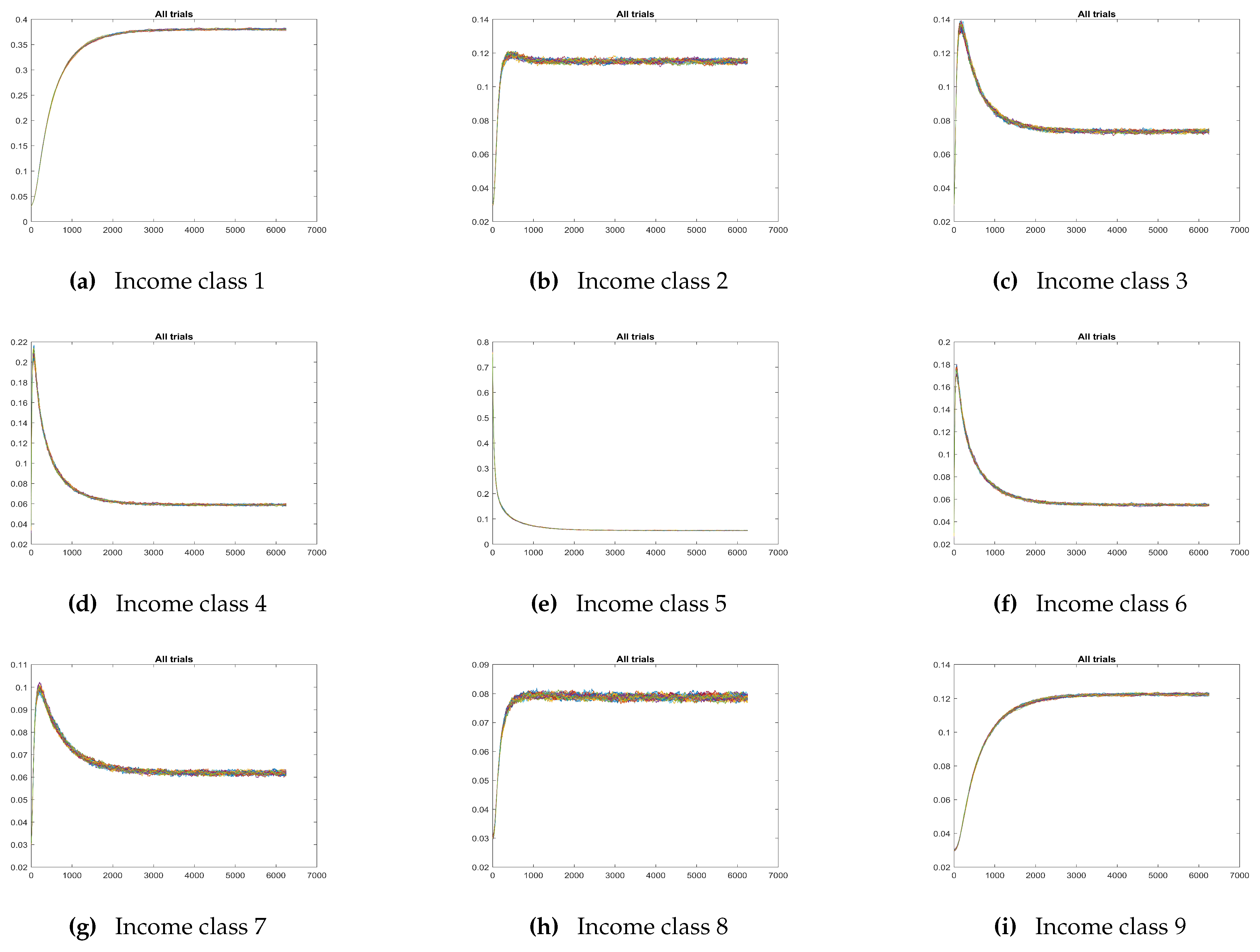
Some results which exhibit features typical of all performed simulations are shown in the Figure 1, Figure 2, Figure 3, Figure 4, Figure 5 and Figure 6. Precisely, the figures from Figure 1, Figure 2, Figure 3 and Figure 4 are relative to the case when $n=9$. Each of the panels in Figure 1 refers to one of the income classes and displays five curves corresponding to the mean over 33 realisations, to the curve obtained adding [respectively, subtracting] at at any time step the standard deviation to [respectively, from] the mean value, and to the curve constructed by taking at any time step the minimum [respectively, the maximum] among the values of the realisations. The panels in Figure 2 refer to the same experiment, and show for each income class the set of all realisations. 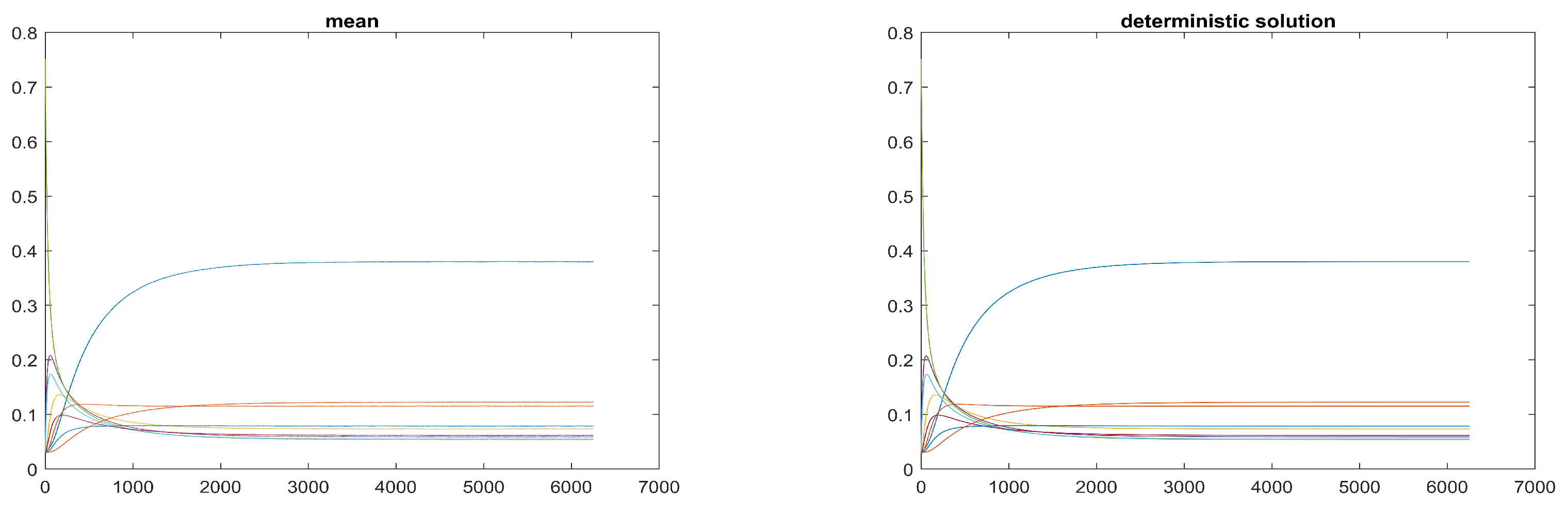The top panel in Figure 3 displays the nine curves respectively obtained by considering at each time step the mean of the values over the 33 realisations, whereas in the bottom panel in the same figure one finds the nine curves corresponding to the components of the solution of the corresponding deterministic problem. The high similarity (possibly, the equality) of the curves in the two panels gives indication of the validity of the model. 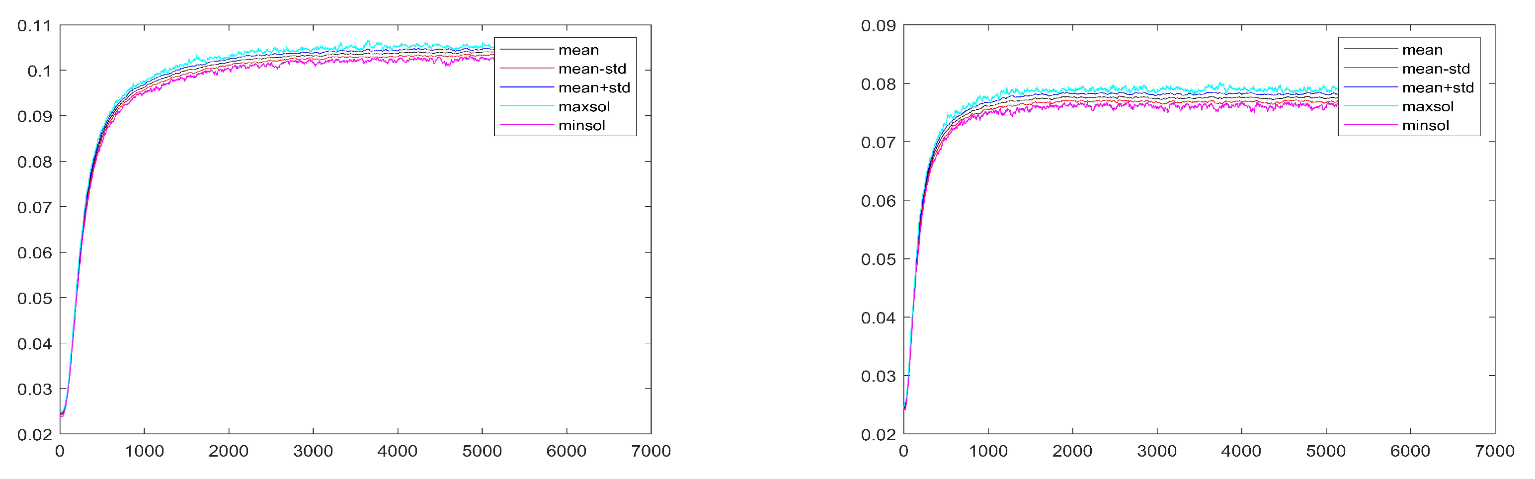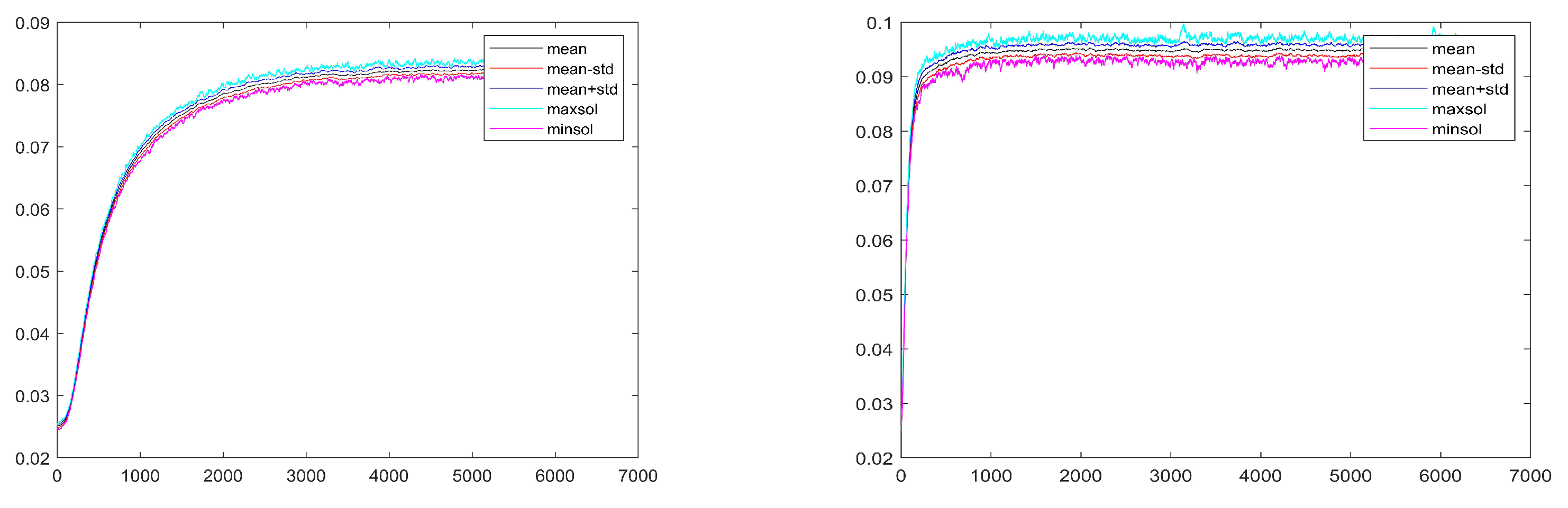The Figure 4 displays the nine curves obtained by considering at each time step the standard deviation of the values over the 33 realisations. The two panels in Figure 5 display the five curves mentioned in the Figure 1 for a case with the same value of the total income, but with $n=11$ in the classes 2 and 10; the same holds for the two panels in Figure 6 with the only difference that they refer to the case in which $n=13$ and the income classes there represented are class 2 and 12 (the second one and the penultimate), those where the fluctuations appear to be the largest one.

By looking at these figures one notices that in the long run the stochastic process modelled by Equation (11), while not leading to an equilibrium, displays fluctuations which do not deviate much from an equilibrium. Such a picture seems to correspond to the appropriate representation of an economic phenomenon.

4. Conclusions

In this paper, building on previous work on kinetic-type models [1], we have developed a novel framework for the description of a market society. This framework is formulated in terms of a nonlinear stochastic differential equation. The main novelty, which can and will be applied to many other problems, consists in the fact that the interaction frequencies of the trading individuals (usually assumed to be constant) are supposed to change at each time step due to the involvement of a normal random variable. More precisely, the interaction frequencies are thought of as the sum of a “deterministic” and a “stochastic” part. In this way, the unavoidable uncertainty that characterizes the real world is naturally incorporated in the model. As a result, credible findings are obtained efficiently.

Possible future perspectives include an attempt to prove the well-posedness of Equation (7), an in-depth examination of continuous data dependence, an investigation into the relationship between the magnitude of the fluctuations and that of the stochastic term in the differential equation, somewhat in the spirit of a stability analysis and a vectorial extension similar to that of [13]. Finally, of course, the development is envisaged of applications of the random variability aspect introduced here to models that arise in various contexts.