MHD Free Convection Flows for Maxwell Fluids over a Porous Plate via Novel Approach of Caputo Fractional Model

Abstract

The ultimate goal of the article is the analysis of free convective flow of an MHD Maxwell fluid over a porous plate. The study focuses on understanding the dynamics of fluid flow over a moving plate in the presence of a magnetic field, where the magnetic lines of force can either be stationary or in motion along the plate. Further, we will investigate the heat and mass transfer characteristics of the system under specific conditions: constant species and thermal conductivity as functions of time. The study involves a symmetric temperature distribution that provides heat on both sides of the plane. Our analysis includes the study of the model for different instances of plate motion and variations in temperature. The fluid dynamics of the system are mathematically described using a system of fractional-order partial differential equations. To make the model independent of geometric units, dimensionless variables are introduced. Moreover, we employ the concept of fractional-order derivative operators in the sense of Caputo, which introduces a fractional dimension to the equations. Additionally, the integral Laplace transform and numerical algorithms are utilized to solve the problem. Finally, by using graphical analysis the contribution of physical parameters on the fluid dynamics is discussed and valuable findings are documented.

1. Introduction

Heat and mass transfer are fundamental principles in engineering that play an important role in a wide range of applications. Having a better understanding of these processes may help to optimize designs, improving efficiency and ensuring the safety and performance of various systems. Heat transfer principles are used in designing engine cooling systems, air conditioning, and exhaust systems in automobiles. Also, these are used in designing thermal protection systems for spacecraft during reentry, as well as cooling systems for aircraft engines. By understanding and applying these principles, engineers can develop innovative solutions to address societal needs, improve efficiency, and advance technology.

Many researchers have shown great interest in studying the applications of magnetic fields in fluid dynamics, as well as exploring the combined study of thermal energy and mass transfer through or in the absence of porous media. In the year 2008, Khan et al. [1] conducted a study examining the control of magnetic field and permeable media on the steady flow of second-grade fluid between two parallel plates. Furthermore, Parinda et al. [2] numerically analyzed the influence of the magnetic field on second-grade fluid through a parallel channel. In that model, they investigated the integrated control of viscoelasticity, magnetic forces, and inertia. In [3], heat and mass transfer phenomena were investigated for magnetohydrodynamic fluid, flowing past a vertical plate; the plate was in motion and had a variable surface temperature and concentration. Further, Seth et al. [4] studied the hydro-magnetic natural convection flow with radiative heat transfer past an accelerated moving vertical plate with variable temperature through a porous medium. Cortell [5] and Raptis et al. [6] examined the flow behavior of an electrically conductive fluid in the presence of a permeable source over a semi-infinite stretched sheet. Additionally, they investigated the effects of a chemical reaction and variable plate motions on the fluid flow. As already mentioned, the dynamics of non-Newtonian fluids through porous media are considered in many studies. Some of the noteworthy investigations include [7,8,9]. Consequently, the field of mass and heat transfer involving magnetohydrodynamic (MHD) flow offers a wealth of captivating subject matter that draws the attention of researchers.

Among various viscoelastic fluid models, Maxwell fluids have garnered significant interest due to their widespread applications in engineering and industry. The constitutive equation of Maxwell fluid is

$$\mathbf{T}=-p\mathbf{I}+\mathbf{S}$$

$$\mathbf{S}+m_1(\dot{\mathit{S}}-L\mathbf{S}-\mathbf{S}{L}^{\ast })=\mu \mathbf{A}$$

where T, p, S, L, $m_1$, $\mu$, and A are, respectively, the Cauchy stress tensor, hydrostatic pressure, extra stress tensor, velocity gradient, relaxation time, dynamic viscosity, and first Rivlin Erickson tensor, and ∗ denotes the transpose.

These fluids are commonly used to study the behavior of certain polymeric fluids. For instance, Refahati et al. in [10] investigated the sound transmission characteristics of a double-walled sandwich magneto-electro-elastic cross-ply layered plate resting on viscoelastic medium in thermal environment. Moreover, the molecular dynamics of gallium nitride nano-sheets under tensile loads are investigated in [11].

Some detailed related work for the case of Newtonian and non-Newtonian fluids can be seen in [12,13,14,15,16,17,18,19,20,21,22,23,24,25,26,27,28,29]) and the references therein. It is pertinent to note that the literature extensively covers the natural convection magnetohydrodynamic (MHD) flow phenomena of various fluids using traditional calculus methods, but they lack memory effects considerations.

More recently, due to the increasing popularity of fractional calculus and the ability to explain the complex dynamics of the model and memory phenomenon [30], the mathematical modeling of the engineering and industrial problems in the setting of fractional calculus has proven to be more realistic and flexible (with memory effects, which are more useful and effective in designing more efficient controls). Due to these characteristics, the fractional calculus modeling is being employed in problems with engineering relevance [31].

Motivated by the above study, the purpose of this manuscript is to investigate the MHD free convective flow of the Maxwell fluid on a vertical permeable plate with constant species concentration. The plate can move along its axis with variable time-dependent velocity. Furthermore, the plate is heated from either sides and a vertically incident magnetic field, which is held either fixed to the fluid or plate is applied to the plate. The problem is modeled via the fractional-order derivative operator (FODO) approach of Caputo. As already mentioned, the fractional-order derivative is a mathematical concept used to describe fractional-order differential equations. The choice of the use of the Caputo fractional model solution method depends on the nature of the problem and the behavior of the system being analyzed. Such a type of model lacks the existing literature, and it has a tendency to exhibit a deep and thorough understanding.

In order to solve our model problem, we will employ the Laplace integral transform method along with the numerical inversion algorithms. Finally, graphical analysis is utilized to investigate the control of the different system parameters, and useful conclusions are recorded.

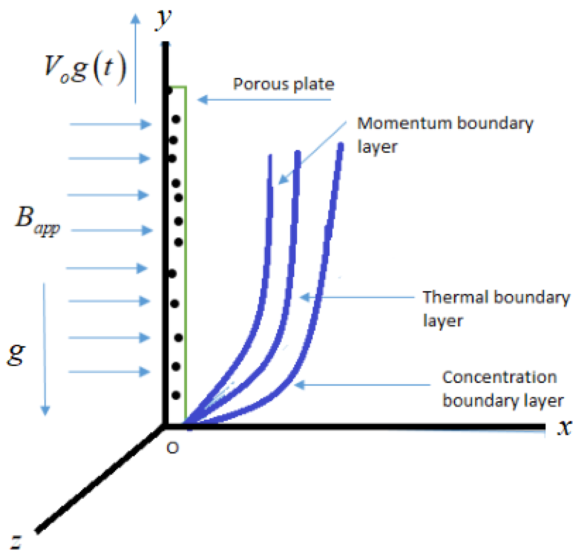
2. Problem Description

This study examines the time-dependent natural convective flow of an electronically conducting Maxwell fluid on an unbounded permeable plate using fractional calculus modeling. The geometry of the the fluid flow model shown in Figure 1. A magnetic field of strength $B_{app}$ (which can be either fixed to the fluid or the plate) is transversely applied. Initially, at $t=0$, both the plate and the fluid are at rest, at the ambient temperature $T_{f\infty }$ and species concentration $C_{\infty }$. At $t=0+$, the concentration remains constant as $C_w$, while the temperature varies according to $T_{f\infty }+T_{fw}f\left(t\right)$. Additionally, the plate starts moving according to a time-dependent function $V_{0}g\left(t\right)$, where $V_0$ is a constant velocity, and $f\left(t\right),g\left(t\right)$ are functions that vanish at $t=0$. Furthermore, the study incorporates the following approximations: Boussinesq’s approximation, viscous dissipation, and Joule heating effect, while neglecting the influence of the induced magnetic field in comparison to the applied magnetic field. The corresponding governing partial differential equations are [24,32,33].

$$\begin{array}{cc}\hfill \frac{\partial V_f(x,t)}{\partial t}& =\frac{1}{\rho }\frac{\partial {\tau }_{ss}(x,t)}{\partial x}+g{\beta }_{T_f}(T_f(x,t)-T_{f\infty })+g{\beta }_C(C(x,t)-C_{\infty })\hfill \\ \hfill & -\frac{{\nu }_k}{K}{V}_f(x,t)-\frac{\sigma B_{app}^2}{\rho }{V}_f(x,t),\hfill \end{array}$$

(1)

$$\begin{array}{cc}\hfill \left(1+m_1\frac{\partial }{\partial t}\right){\tau }_{ss}(x,t)& ={\nu }_d\frac{\partial V_f(x,t)}{\partial x};x,t>0.\hfill \end{array}$$

(2)

where $V_f(x,t)$ denotes the fluid velocity, and ${\tau }_{ss}(x,t)$ represents the shear stress.

If the magnetic lines of forces are fixed relative to the fluid (MFFRF) then Equation (1) is accurate, whereas for the case when the magnetic lines of forces are fixed relative to the plate (MFFRP), then Equation (1) is modified as [34,35]

$$\begin{array}{cc}\hfill \frac{\partial V_f(x,t)}{\partial t}& =\frac{1}{\rho }\frac{\partial {\tau }_{ss}(x,t)}{\partial x}+g{\beta }_{T_f}(T_f(x,t)-T_{f\infty })+g{\beta }_C(C(x,t)-C_{\infty })\hfill \\ \hfill & -\frac{{\nu }_k}{K}{V}_f(x,t)-\frac{\sigma B_{app}^2}{\rho }(V_f(x,t)-ϵV_{0}g\left(t\right));x,t>0.\hfill \end{array}$$

(3)

Into the above relations, the parameter $ϵ$ is 0 for MFFRF and 1 for MFFRP.

Solving (2) and (3) to eliminate ${\tau }_{ss}(x,t)$ from Equation (3), we obtain

$$\begin{array}{cc}\hfill \left(1+m_1\frac{\partial }{\partial t}\right)\frac{\partial V_f(x,t)}{\partial t}& ={\nu }_k\frac{{\partial }^2{V}_f(x,t)}{\partial x^2}+\left(1+m_1\frac{\partial }{\partial t}\right)g({\beta }_{T_f}(T_f(x,t)-T_{f\infty })\hfill \\ & +{\beta }_C(C(x,t)-C_{\infty }))-\frac{{\nu }_k}{K}{V}_f(x,t)-\frac{\sigma B_{app}^2}{\rho }(V_f(x,t)-ϵV_{0}g\left(t\right)).\hfill \end{array}$$

(4)

Moreover, heat and concentration equations are

$$\begin{array}{cc}\hfill \rho c_p\frac{\partial T_f(x,t)}{\partial t}& ={\theta }_k\frac{{\partial }^2{T}_f(x,t)}{\partial x^2}-\frac{\partial q_r}{\partial x},\hfill \end{array}$$

(5)

$$\begin{array}{cc}\hfill \frac{\partial C(x,t)}{\partial t}& =D_m\frac{{\partial }^{2}C(x,t)}{\partial x^2}-C_R(C(x,t)-C_{\infty }).\hfill \end{array}$$

(6)

The related initial conditions for the problem when $x\ge 0$ are

$$\begin{array}{cc}\hfill V_f(x,t)& =0,T_f(x,t)=T_{f\infty },C(x,t)=C_{\infty },{\tau }_{ss}(x,t)=0,\mathrm{at}t=0.\hfill \end{array}$$

(7)

The boundary conditions related to our model are described as, for $t>0$,

$$\begin{array}{cc}\hfill V_f(x,t)& =V_{0}g\left(t\right),T_f(x,t)=T_{f\infty }+T_{fw}f\left(t\right),C(x,t)=C_w,\mathrm{at}x=0,\hfill \end{array}$$

(8)

$$\begin{array}{c}\hfill V_f(x,t)<\infty ,T_f(x,t)\to T_{f\infty },C(x,t)\to C_{\infty },\mathrm{as}x\to \infty .\end{array}$$

(9)

Here, the condition $V_f(x,t)<\infty$ as $x\to \infty$ shows that far away from the plate, the velocity of the fluid is finite (rather than zero), while temperature and concentration are constant.

Using the Rosseland diffusion approximation (for an optically thick fluid) [36,37]

$$\begin{array}{cc}\hfill q_r& =-\frac{4}{3}\frac{\sigma }{k_R}\frac{\partial T_f^4}{\partial x}\hfill \end{array}$$

(10)

and for the case $\mid T_f-T_{f\infty }\mid \ll 0$, the following is a simplified version of the Equation (5) [38,39]

$$\begin{array}{cc}\hfill P{r}_{eff}\frac{\partial T_f(x,t)}{\partial t}& =\frac{{\partial }^2{T}_f(x,t)}{\partial x^2};x,t>0,\hfill \end{array}$$

(11)

where

$$\begin{array}{cc}\hfill P{r}_{eff}& =\frac{P_r}{1+R_c},P_r=\frac{{\nu }_d{c}_p}{{\theta }_k}\mathrm{and}{R}_c=\frac{16}{3}\frac{\sigma }{{\theta }_k{k}_R}{T}_{f\infty }^3.\hfill \end{array}$$

To make the problem free from geometric regime, the subsequent dimensionless quantities are introduced [40,41].

$$\begin{array}{c}\hfill x^{\ast }=\frac{V_0}{{\nu }_k}x,t^{\ast }=\frac{V_0^2}{{\nu }_k}t,V_f^{\ast }=\frac{V_f}{V_0},T_f^{\ast }=\frac{T_f-T_{f\infty }}{T_{fw}},C^{\ast }=\frac{C-C_{\infty }}{C_w-C_{\infty }},K^{\ast }=\left(\frac{{\nu }_k}{V_0}\right)\frac{1}{K},\\ \hfill {\beta }^{\ast }=\frac{{\nu }_k}{V_0^2}\beta ,R^{\ast }=\frac{{\nu }_k}{V_0^2}R,m_1^{\ast }=\frac{V_0^2}{{\nu }_k}{m}_1,S^{\ast }=\frac{S}{\rho V_0^2},f^{\ast }\left(t^{\ast }\right)=f\left(\frac{{\nu }_k}{V_0^2}{t}^{\ast }\right),g^{\ast }\left(t^{\ast }\right)=g\left(\frac{{\nu }_k}{V_0^2}{t}^{\ast }\right).\end{array}$$

(12)

The dimensionless system of PDEs Equations (4), (6), and (11), after dropping ‘*’ notation, becomes

$$\begin{array}{cc}\hfill \left(1+m_1\frac{\partial }{\partial t}\right){\tau }_{ss}(x,t)& =\frac{\partial V_f(x,t)}{\partial x}.\hfill \end{array}$$

(13)

$$\begin{array}{cc}\hfill \left(1+m_1\frac{\partial }{\partial t}\right)\frac{\partial V_f(x,t)}{\partial t}& =\frac{{\partial }^2{V}_f(x,t)}{\partial x^2}+\left(1+m_1\frac{\partial }{\partial t}\right)[(T_f(x,t)+N_{b}C(x,t))\hfill \\ & -K{V}_f(x,t)-M_g(V_f(x,t)-ϵg\left(t\right))].\hfill \end{array}$$

(14)

$$\begin{array}{cc}\hfill P_{reff}\frac{\partial T_f(x,t)}{\partial t}& =\frac{{\partial }^2{T}_f(x,t)}{\partial x^2}.\hfill \end{array}$$

(15)

$$\begin{array}{cc}\hfill \frac{\partial C(x,t)}{\partial t}& =\frac{1}{S_c}\frac{{\partial }^{2}C(x,t)}{\partial x^2}-C_{R}C(x,t).\hfill \end{array}$$

(16)

Moreover, the initial and boundary conditions associated with the fluid dynamics of our model in dimensionless relations are

$$\begin{array}{cc}\hfill V_f(x,t)& =0,T_f(x,t)=0,C(x,t)=0,{\tau }_{ss}(x,t)=0,\mathrm{at}t=0,x\ge 0.\hfill \end{array}$$

(17)

$$\begin{array}{cc}\hfill V_f(x,t)& =g\left(t\right),T_f(x,t)=f\left(t\right),C(x,t)=1,\mathrm{at}x=0,‘t>0.\hfill \end{array}$$

(18)

$$\begin{array}{c}\hfill V_f(x,t)<\infty ,T_f(x,t)\to 0,C(x,t)\to 0,\mathrm{as}x\to \infty .\end{array}$$

(19)

3. Fractional Analogue

As already mentioned, the mathematical modeling of engineering and industrial problems in the setting of fractional calculus has been proven to be more realistic and flexible, with memory effects, which are more useful and effective in designing more efficient controls. Due to these characteristics, fractional calculus modeling is being employed in problems with engineering relevance. As the first step towards the fractional analogue of our model, we will employ the Caputo FODO on Equations (13)–(16) (by replacing the partial derivative with respect to time by the FODO counterpart)

$$\begin{array}{cc}\hfill \left(1+m_1^C{D}_t^{\alpha }\right)\frac{\partial V_f(x,t)}{\partial t}& =\frac{{\partial }^2{V}_f(x,t)}{\partial x^2}+\left(1+m_1^C{D}_t^{\alpha }\right)[T_f(x,t)+N_{b}C(x,t)-K{V}_f(x,t)\hfill \\ \hfill & -M_g(V_f(x,t)-ϵg\left(t\right))],\hfill \end{array}$$

(20)

$$\begin{array}{cc}\hfill P{r}_{eff}{}^C{D}_t^{\alpha }{T}_f(x,t)& =\frac{{\partial }^2{T}_f(x,t)}{\partial x^2},\hfill \end{array}$$

(21)

$$\begin{array}{cc}\hfill {}^C{D}_t^{\alpha }C(x,t)& =\frac{1}{S_c}\frac{{\partial }^{2}C(x,t)}{\partial x^2}-C_{R}C(x,t),\hfill \end{array}$$

(22)

$$\begin{array}{cc}\hfill \left(1+m_1^C{D}_t^{\alpha }\right){\tau }_{ss}(x,t)& =\frac{\partial V_f(x,t)}{\partial x}.\hfill \end{array}$$

(23)

where ${}^C{D}_t^{\alpha }$ is known as Caputo FODO [42] defined as

$$\begin{array}{cc}\hfill {}^C{D}_t^{\alpha }h(x,t)& =\frac{1}{\mathsf{\Gamma }(1-\alpha )}{\int }_0^t\frac{h^{\prime }(x,\varrho )}{{(t-\varrho )}^{\alpha }}d\varrho ,\alpha \in (0,1),\hfill \end{array}$$

(24)

whereas the Laplace transform (LT) of Caputo FODO is

$$\begin{array}{cc}\hfill L\left({}^C{D}_t^{\alpha }h(x,t)\right)& =p^{\alpha }L\left(h(x,t)\right)-p^{(\alpha -1)}h(x,0).\hfill \end{array}$$

(25)

4. Mathematical Computation

4.1. Computation for Temperature Profile

Now, employing the LT on temperature Equation (21) and customizing the requisite initial conditions, we obtain

$$\begin{array}{cc}\hfill \frac{{\partial }^2{\overline{T}}_f(x,p)}{\partial x^2}-P{r}_{eff}{p}^{\alpha }{\overline{T}}_f(x,p)& =0.\mathrm{as}{T}_f(x,0)=0.\hfill \end{array}$$

(26)

Moreover, the Laplace transform of the boundary conditions appears as

$$\begin{array}{c}\hfill {\overline{T}}_f(0,p)=f\left(p\right),{\overline{T}}_f(x,p)\to 0\mathrm{as}x\to \infty .\end{array}$$

(27)

The final computation for the Equation (26) constraint to Equation (27) leads us to

$$\begin{array}{cc}\hfill {\overline{T}}_f(x,p)& =f\left(p\right)e^{-x\sqrt{P{r}_{eff}{p}^{\alpha }}}.\hfill \end{array}$$

(28)

Now, in order to measure the rate of heat transfer, we compute the Nusselt number, defined by

$$\begin{array}{cc}\hfill N_u& =-L^{-1}\left\{\frac{\partial {\overline{T}}_f(x,p)}{\partial x}{\mid }_{x=0}\right\},\hfill \end{array}$$

$$\begin{array}{cc}\hfill & =L^{-1}\left\{\sqrt{P{r}_{eff}{p}^{\alpha }}f\left(p\right)\right\},\hfill \end{array}$$

$$\begin{array}{cc}\hfill & =\sqrt{P{r}_{eff}}{L}^{-1}\left\{\sqrt{p^{\alpha }}f\left(p\right)\right\}.\hfill \end{array}$$

(29)

4.2. Computation for Concentration Profile

Similarly, employing the LT on the FOPDE for concentration Equation (22), and making use of the initial conditions, we obtain

$$\begin{array}{c}\hfill \frac{{\partial }^2\overline{C}(x,p)}{\partial x^2}-S_c(p^{\alpha }+C_R)\overline{C}(x,p)=0,\end{array}$$

(30)

along with transformed boundary conditions as

$$\begin{array}{c}\hfill \overline{C}(0,p)=\frac{1}{p},\overline{C}(x,p)\to 0\mathrm{as}x\to \infty .\end{array}$$

(31)

Hence, the obtained solution for the concentration profile is

$$\begin{array}{cc}\hfill \overline{C}(x,p)& =\frac{1}{p}{e}^{-x\sqrt{S_c\left(p^{\alpha }+C_R\right)}}.\hfill \end{array}$$

(32)

Furthermore, the rate of mass transfer is measured by Sherwood number, defined as

$$\begin{array}{c}\hfill S_h=-L^{-1}\left\{\frac{\partial \overline{C}(x,p)}{\partial x}{\mid }_{x=0}\right\},\end{array}$$

$$\begin{array}{c}\hfill S_h=\sqrt{S_c}{L}^{-1}\left\{\frac{\sqrt{p^{\alpha }+C_R}}{p}\right\}.\end{array}$$

(33)

4.3. Computation for Velocity Profile

Implementing the LT to Equation (22), by utilizing the initial conditions, we obtain the following expression:

$$\begin{array}{cc}\hfill \frac{{\partial }^2{\overline{V}}_f(x,p)}{\partial x^2}-{\beta }_1(p+H){\overline{V}}_f(x,p)& =-{\beta }_1\left({\overline{T}}_f(x,p)+N_b\overline{C}(x,p)+M_gϵg\left(p\right)\right),\hfill \end{array}$$

(34)

where ${\beta }_1=\left(1+m_1{p}^{\alpha }\right)$, $H=K+M_g$.

$$\begin{array}{cc}\hfill \frac{{\partial }^2{\overline{V}}_f(x,p)}{\partial x^2}-{\beta }_2{\overline{V}}_f(x,p)& =-{\beta }_1\left({\overline{T}}_f(x,p)+N_b\overline{C}(x,p)+M_gϵg\left(p\right)\right),\hfill \end{array}$$

with ${\beta }_2={\beta }_1(p+H)$.

Incorporating the value of the ${\overline{T}}_f(x,p)$ from Equation (28) and $\overline{C}(x,p)$ from Equation (32) into the last expression leads to

$$\begin{array}{cc}\hfill \frac{{\partial }^2{\overline{V}}_f(x,p)}{\partial x^2}-{\beta }_2{\overline{V}}_f(x,p)& =-{\beta }_1\left(f\left(p\right)e^{-x\sqrt{P{r}_{eff}{p}^{\alpha }}}+N_b\frac{1}{p}{e}^{-x\sqrt{S_c\left(p^{\alpha }+C_R\right)}}+M_gϵg\left(p\right)\right),\hfill \end{array}$$

(35)

along with the boundary conditions

$$\begin{array}{c}\hfill {\overline{V}}_f(0,p)=g\left(p\right),{\overline{V}}_f(x,p)<\infty ,\mathrm{as}x\to \infty .\end{array}$$

(36)

The solution of (35) subject to (36) yields

$$\begin{array}{cc}\hfill {\overline{V}}_f(x,p)& =g\left(p\right)e^{-x\sqrt{(1+m_1{p}^{\alpha })(p+H)}}+\frac{(1+m_1{p}^{\alpha })f\left(p\right)}{P_{reff}{p}^{\alpha }-(1+m_1{p}^{\alpha })(p+H)}\left(e^{-x\sqrt{(1+m_1{p}^{\alpha })(p+H)}}-e^{-x\sqrt{P{r}_{eff}{p}^{\alpha }}}\right)\hfill \\ \hfill & +\frac{(1+m_1{p}^{\alpha })N_b}{p[S_c(p^{\alpha }+C_R)-(1+m_1{p}^{\alpha })(p+H)]}\left(e^{-x\sqrt{(1+m_1{p}^{\alpha })(p+H)}}-e^{-x\sqrt{S_c(s^{\alpha }+C_R)}}\right)\hfill \\ \hfill & +\frac{M_gϵg\left(p\right)}{p+H}\left(1-e^{-x\sqrt{(1+m_1{p}^{\alpha })(p+H)}}\right).\hfill \end{array}$$

(37)

4.4. Computation for Shear Stress

By employing the LT on Equation (23) and incorporating the associated initial condition, we obtain

$$\begin{array}{cc}\hfill \left(1+m_1{p}^{\alpha }\right){\overline{\tau }}_{ss}(x,p)& =\frac{\partial {\overline{V}}_f(x,p)}{\partial x},\hfill \end{array}$$

$$\begin{array}{cc}\hfill {\overline{\tau }}_{ss}(x,p)& =\left(\frac{1}{1+m_1{p}^{\alpha }}\right)\frac{\partial {\overline{V}}_f(x,p)}{\partial x}.\hfill \end{array}$$

(38)

Differentiating Equation (37) with respect to x and using it into Equation (38) leads to the computation for shear stress as

$$\begin{array}{cc}\hfill {\overline{\tau }}_{ss}(x,p)& =-g\left(p\right)\sqrt{\frac{(p+H)}{1+m_1{p}^{\alpha }}}{e}^{-x\sqrt{(1+m_1{p}^{\alpha })(p+H)}}+\frac{(1+m_1{p}^{\alpha })f\left(p\right)}{P_{reff}{p}^{\alpha }-(1+m_1{p}^{\alpha })(p+H)}\hfill \\ \hfill & \times \left(-\sqrt{\frac{(p+H)}{1+m_1{p}^{\alpha }}}{e}^{-x\sqrt{(1+m_1{p}^{\alpha })(p+H)}}+\frac{\sqrt{P{r}_{eff}{p}^{\alpha }}}{1+m_1{p}^{\alpha }}{e}^{-x\sqrt{P{r}_{eff}{p}^{\alpha }}}\right)\hfill \\ \hfill & +\frac{(1+m_1{p}^{\alpha })N}{p[S_c(p^{\alpha }+C_R)-(1+m_1{p}^{\alpha })(p+H)]}\hfill \\ \hfill & \times \left(-\sqrt{\frac{(p+H)}{1+m_1{p}^{\alpha }}}{e}^{-x\sqrt{(1+m_1{p}^{\alpha })(p+H)}}+\frac{\sqrt{S_c(p^{\alpha }+C_R)}}{(1+m_1{p}^{\alpha })}{e}^{-x\sqrt{S_c(p^{\alpha }+C_R)}}\right)\hfill \\ \hfill & +\frac{M_gϵg\left(p\right)}{\sqrt{(1+m_1{p}^{\alpha })(p+H)}}{e}^{-x\sqrt{(1+m_1{p}^{\alpha })(p+H)}}.\hfill \end{array}$$

(39)

Finally, to obtain the solution for temperature, concentration, and velocity, we need to apply inverse Laplace transform, which is somewhat tedious; it is not much of a problem for (28) and (32) but really is a problem for our main results (37) and (39). This problem can be solved by employing some numerical Laplace inversion algorithms like Stehfest’s and Tzou’s numerical algorithms [43,44]. Stehfest’s algorithm representation is

$$\begin{array}{c}\hfill \phi (\varsigma ,t)=\frac{lo{g}_e\left(2\right)}{t}\sum _{n=1}^{2q}{h}_j\overline{\phi }\left(\varsigma ,n\frac{ln\left(2\right)}{t}\right),\end{array}$$

where q is a positive integer and

$$\begin{array}{cc}\hfill h_j& ={(-1)}^{j+q}\sum _{i=\left[\frac{j+1}{2}\right]}^{min(j,q)}\frac{i^q\left(2i\right)!}{(q-i)!i!(i-1)!(j-i)!(2i-j)!}.\hfill \end{array}$$

Furthermore, Tzou’s numerical inversion algorithm for LT is

$$\begin{array}{cc}\hfill \phi (\varsigma ,t)& =\frac{e^{4.7}}{t}\left[\frac{1}{2}\overline{\phi }\left(\varsigma ,\frac{4.7}{t}\right)+Re\left\{\sum _{n=1}^N{(-1)}^n\overline{\phi }\left(\varsigma ,\frac{4.7+k\pi \sqrt{(}-1)}{t}\right)\right\}\right].\hfill \end{array}$$

It is pertinent to mention that, in the present problem, we will employ Stehfest’s algorithm for Laplace inversion of our results.

5. Graphical Analysis and Discussion

In this section, in order to obtain the in-depth analysis of the relevant variables related to the flow of fluid, we conduct a graphical analysis. The influence of the system parameters is analyzed along with their physical significance. More specifically, special attention is paid to investigating the control of the system parameters on the dynamics of our model in two scenarios, namely, MFFRF and MFFRP.

Figure 2 is prepared to investigate the effect of $\alpha$ (the FO parameter) on the concentration profiles. It is observed that an increase in the FO parameter results in an increase in the diffusion profiles that strengthens the boundary layer thickness and results in the increase in concentration profile.

Next, in order to assess the impact of Schmidt number $S_c$ on profiles of concentration, Figure 3 is prepared. It is observed that the increase in momentum diffusivity relative to mass diffusivity depreciates the concentration profile of the fluid. The reason is that, since $S_c$ depends on Brownian diffusivity by inverse relation, the higher values of $S_c$ lower the Brownian diffusivity, resulting in the lowering of the concentration profiles.

The control of chemical reaction parameter on concentration profiles is examined in the Figure 4. It is noticed that concentration profiles experience a decrement with the increase in $C_R$. The reason is that the increase in $C_R$ reduces the buoyancy effects, which leads to a decrease in the fluid’s velocity, and consequently a decrease in concentration profiles is observed.

Further, the control of $\alpha$ on the temperature profiles is studied in Figure 5, and it is shown that $T(\varsigma ,t)$ increases for increasing values of $\alpha$. The reason is that the increase in the value of $\alpha$ increases the boundary layer thickness; hence, the temperature profile is raised. Moreover, an investigation is carried out for two types of temperature distributions, namely, for $f\left(t\right)=H\left(t\right)(1-a{e}^{-bt})$ and $f\left(t\right)=H\left(t\right)$, and it is noted that the temperature profiles are significant for $f\left(t\right)=H\left(t\right)$.

For understanding the influence of $P_{reff}$ on the temperature profiles, Figure 6 is prepared, and it is observed that the presence of higher values of the effective Prandtl number significantly lowers the temperature profiles. The main reason is that the effective Prandtl number and radiations are inversely proportional to each other.

The way in which the velocity profiles are influenced by variation in $\alpha$ ? is recorded in Figure 7 and Figure 8 for the cases when $g\left(t\right)=t^{\beta }$ and $g\left(t\right)=H\left(t\right)sin\left(\omega t\right)$. As observed above, the velocity profiles are raised for increasing values of $\alpha$ because the increase in alpha makes the boundary layer thick, resulting in a boost in the fluid flow. Also, the fluid’s correspondence to the case MFFRP is higher than in the situation when MFFRF is observed.

The control of Schmidt number $S_c$ on the fluid’s velocity is examined in Figure 9. It can be seen that velocity decreases with the increase in Schmidt number. Because $S_c$ is a transport parameter, any increase in it results in the depreciation of concentration of the fluid that ultimately decreases the influences of concentration buoyancy and leads to slowness in fluid flow.

As ($P_r$) controls momentum and boundary layer thickness, the influence of $P_r$ on velocity profiles of fluid is examined in Figure 10. As is evident from the velocity profiles, the increase in the values of $P_r$ reduces the flow velocity of fluid because the increase in the values of $P_r$ reduces the thermal conductivity and consequently it decreases the boundary layer thickness.

Furthermore, the influence of $M_g$ (the magnetic parameter) on the dynamics of fluid is investigated in Figure 11. It is recorded that both the velocity profiles and the boundary layer thickness decrease for increasing values of $M_g$. As the transverse magnetic field on the flowing fluid produces a Lorentz force, a kind of resistive force quite likely the drag-force. Moreover, the strength of the Lorentz force depends upon the strength of the magnetic field; hence, fluid flow is slow for larger values of $M_g$. The influence is more significant for the case MFFRF than MFFRP. Also, the profiles of velocity are significantly higher in the situation when $g\left(t\right)=t^{\beta }$ other than the case when $g\left(t\right)$ is a sinusoidal function of time.

As the Maxwell fluids involves the relaxation time parameter $m_1$, the influence of this parameter on the dynamics of the fluid flow are illustrated in Figure 12 and Figure 13. It is observed that fluid velocity tends to decrease for increasing values of $m_1$ for both scenarios when MFFRP and MFFRF, but evidently the flow profiles for MFFRP are higher than the case of MFFRF and the effects of $m_1$ are quite a lot smaller at small time values.

The influence of K (the porosity parameter) is recorded in Figure 14 and Figure 15. From the plots, it is noticed that increasing values of K bring a slow depreciation in the magnitude of the flow velocity of fluid and indicate Darcy flow. Moreover, the trends are significant when MFFRP other than situation when MFFRF.

6. Conclusions

In this study we examined the free convective flow of MHD Maxwell fluid over a porous plate with the aim of focusing on comprehending fluid dynamics over a moving plate in the presence of a magnetic field, where magnetic lines of force can be stationary or in motion along the plate. The mathematical representation employs fractional-order PDEs, incorporating the fractional-order derivative operator in the sense of Caputo, introducing the fractional dimensions to the equation. Moreover, our investigation was under specific conditions involving constant species and time-dependent thermal conductivity. The analysis considered symmetrical temperature distribution, offering heat on both sides of the plate. Various plate motion scenarios and temperature changes were explored. The findings concluded from the evidence and arguments presented in the research study are summarized as follows:

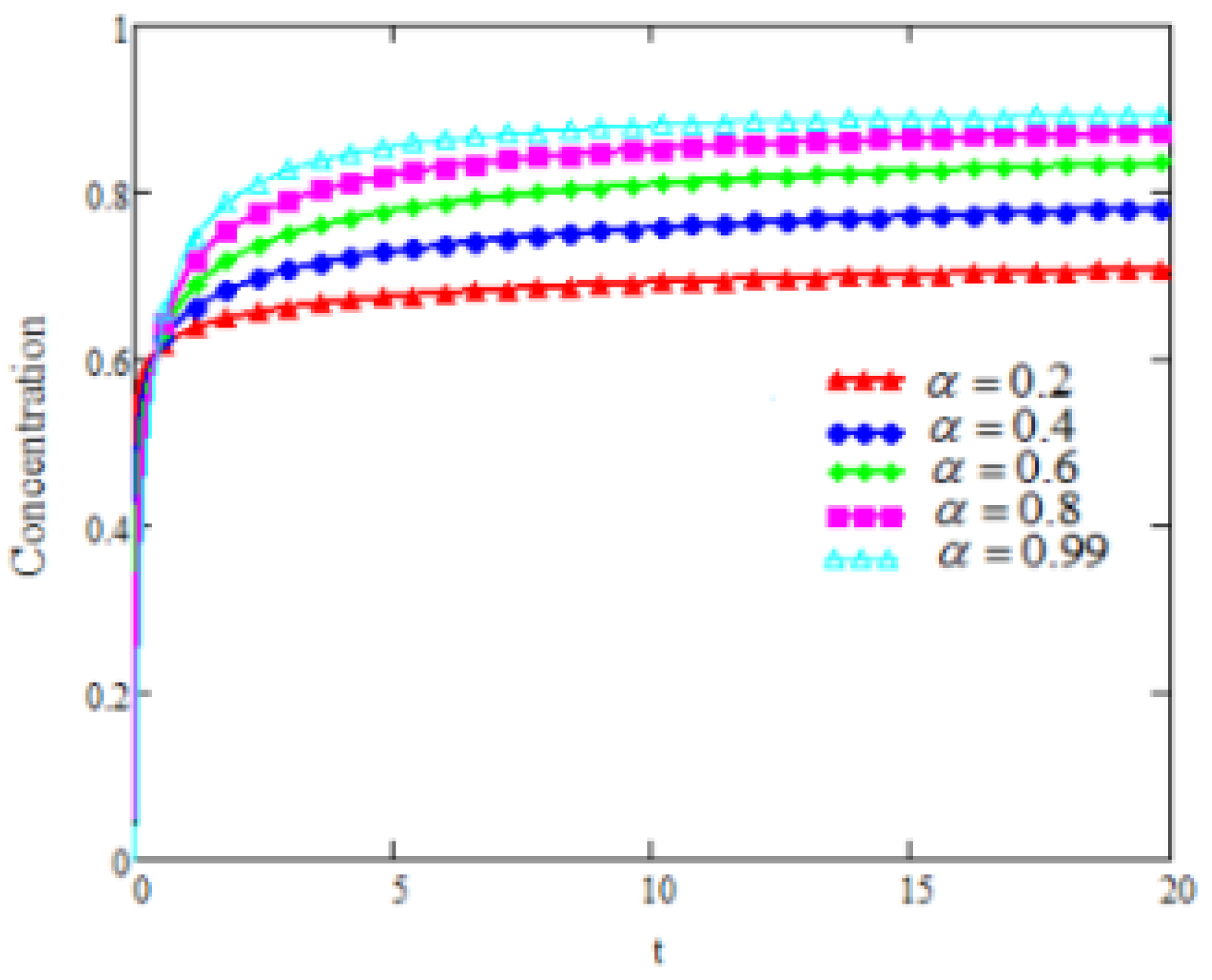
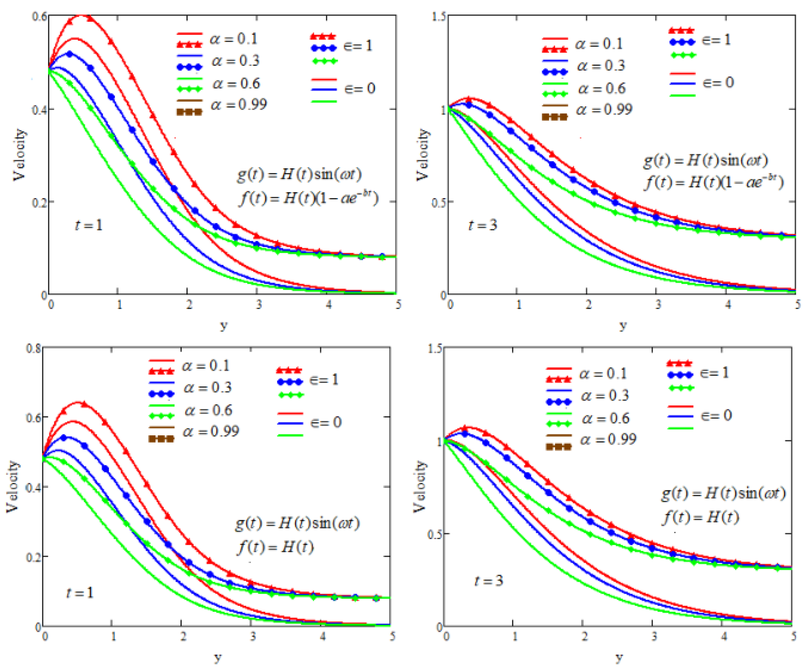
• With respect to the increasing values of the fractional-order parameter, the profiles of concentration, temperature, and velocity exhibit increasing trends.
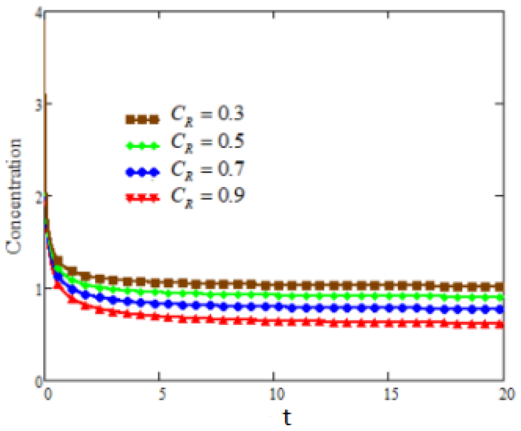
• As the value of $S_c$ rises, there is a corresponding decrease in the concentration profile of the fluid.
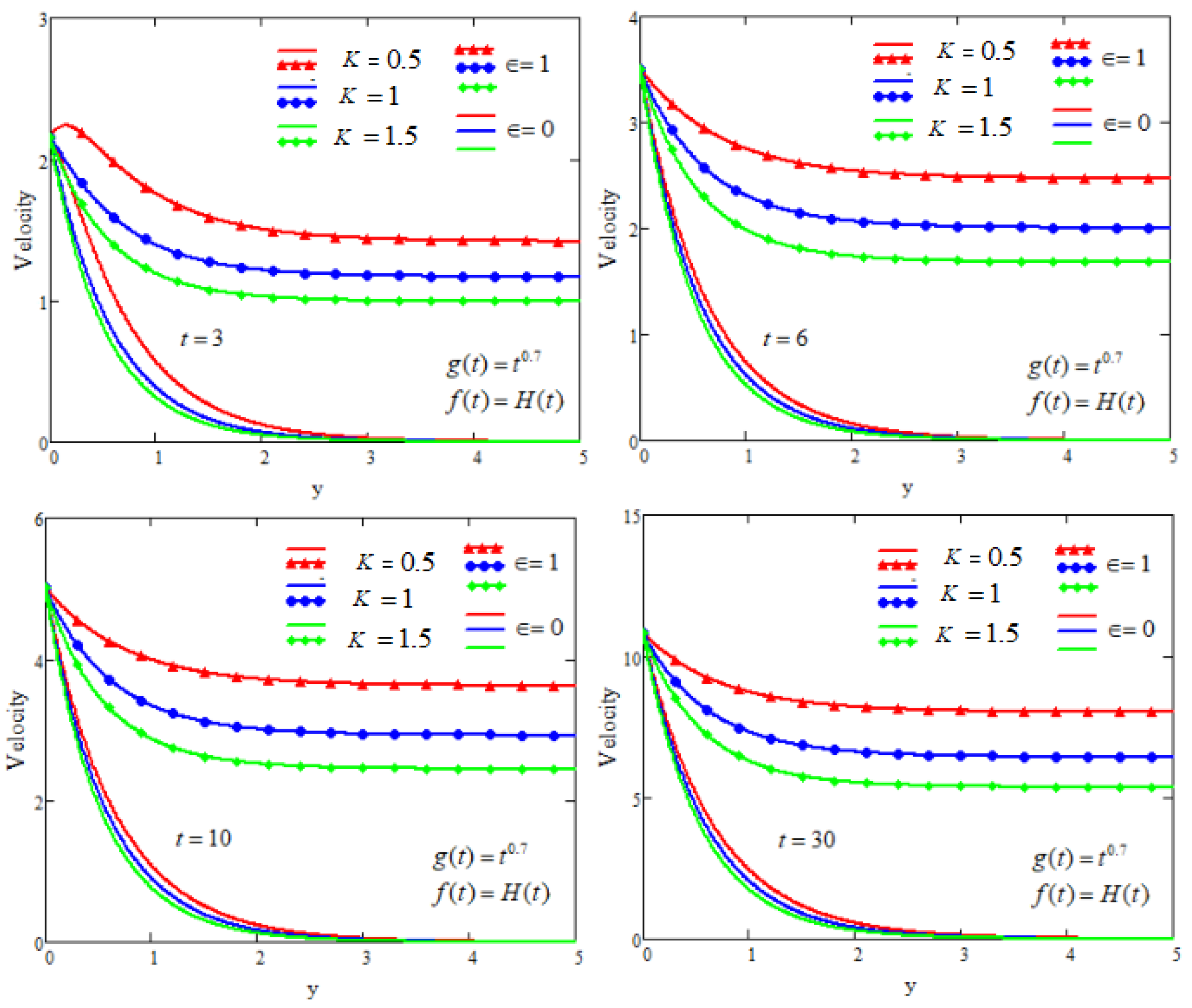
• A higher value of the chemical reaction parameter catalyzes a decline in the fluid velocity.
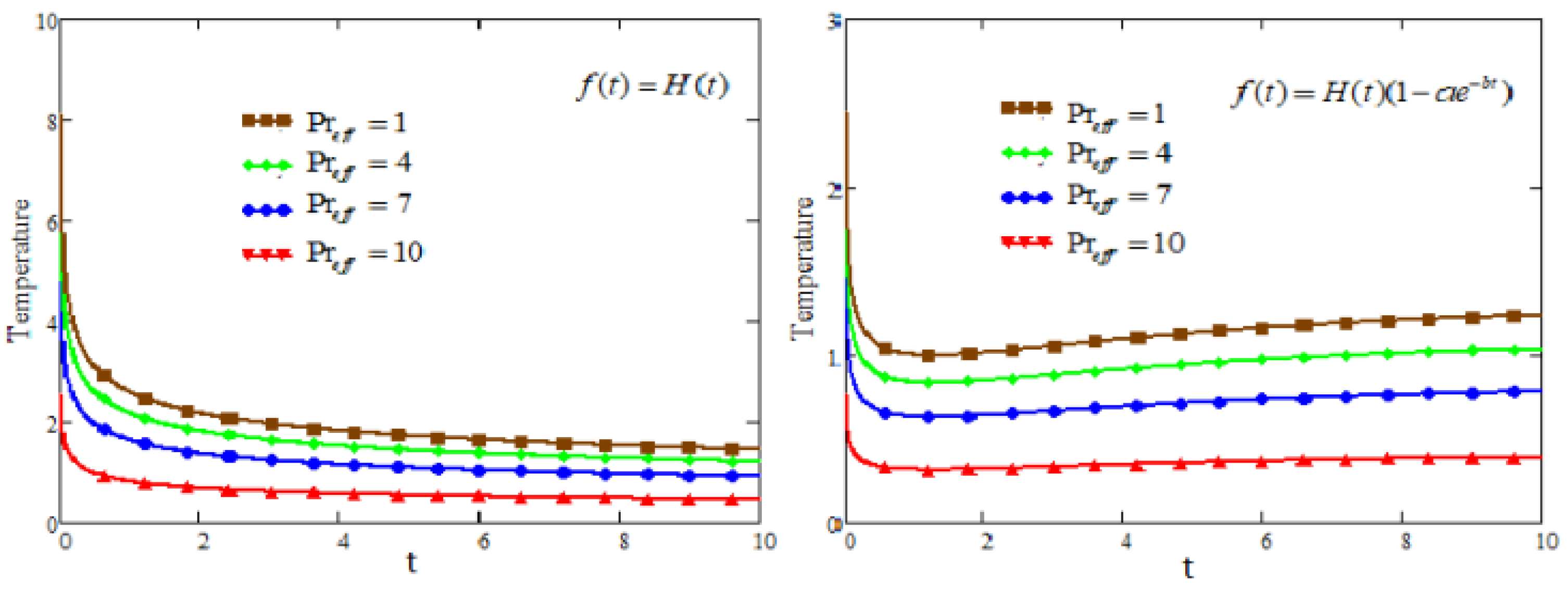
• As the effective Prandtl number increases, the rate of heat transfer also rises, but it gradually diminishes over time.
• Increasing the values of $P_r$ leads to a decrease in temperature profiles.
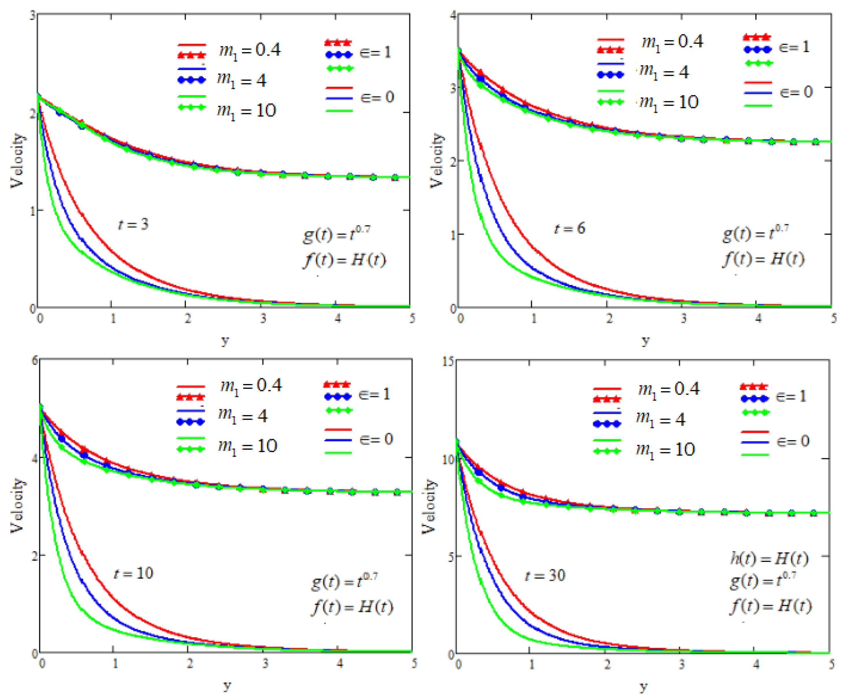
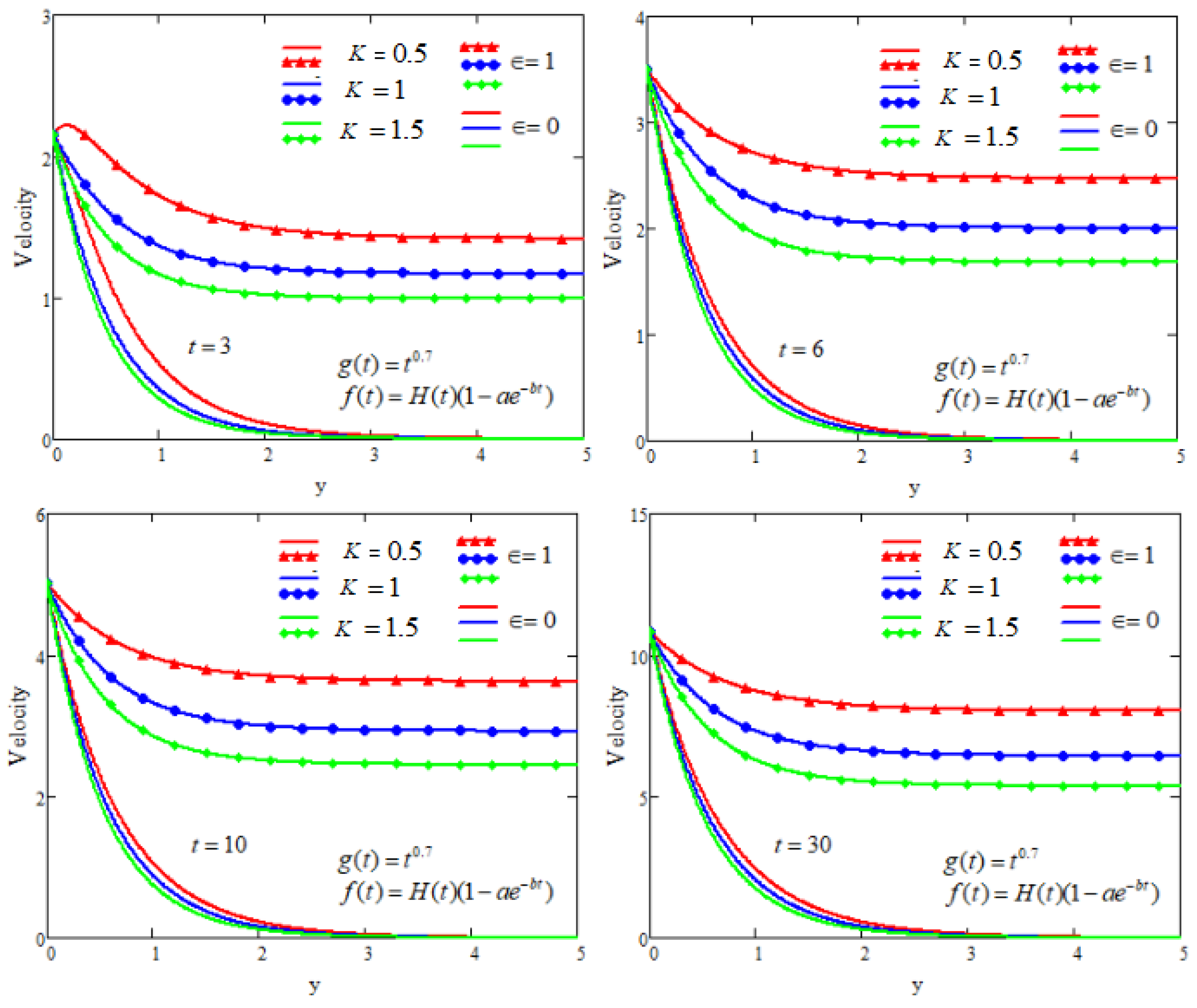
• The fluid velocity decreases as the relaxation time and porosity parameters increase, and their control weakens over time.
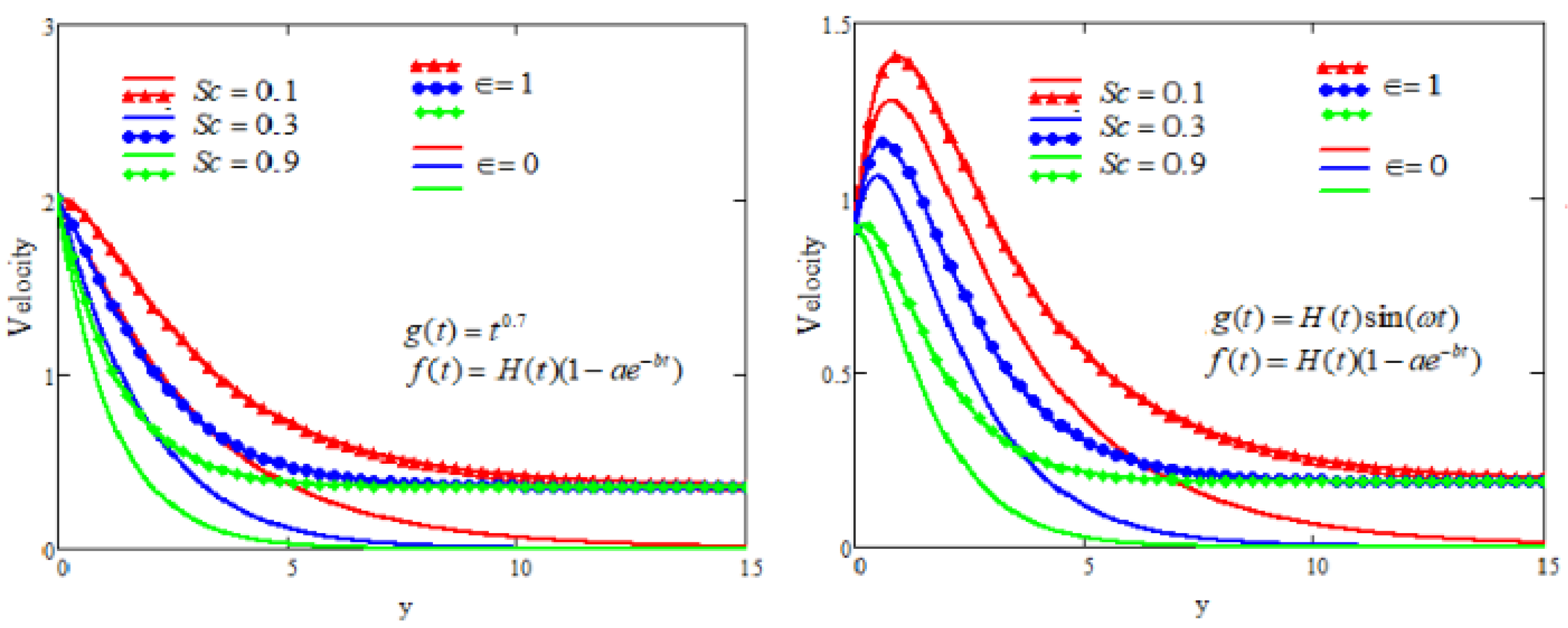
• With the increase in the Schmidt number, the velocity profiles depreciate.
• Strengthening the Prandtl number weakens the magnitude of the velocity profiles.
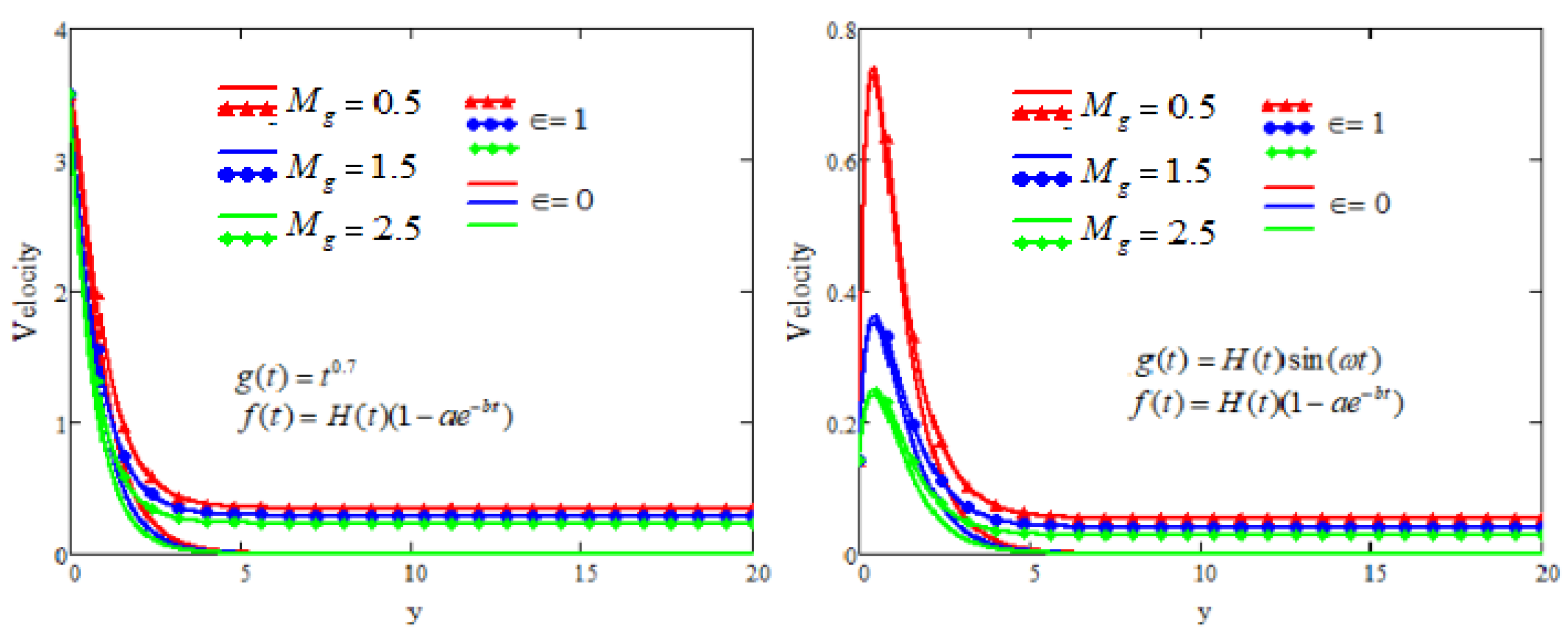
• With an increase in the values of the magnetic parameter, the boundary layer thickness becomes narrower, causing a corresponding decrease in the flow velocity.
• In the case when MFFRP, the profiles of fluid velocity are significantly greater in comparison to the scenario when MFFRF.

7. Future Works

For future work, we will extend this methodology for doing a comparative analysis of the proposed problem using various definitions of fractional derivative operators.

References

1. Khan, I.; Ellahi, R.; Fectecau, C. Some MHD flows of second grade fluid throgh the prous medium. J. Porous Media 2008, 11, 389–400. [Google Scholar]
2. Parida, S.K.; Panda, S.; Acharya, M.K. Magnetrohydrodynamics (MHD) flow of a second grade fluid in a channel with porous wall. Meccanica 2011, 46, 1093–1102. [Google Scholar] [CrossRef]
3. Javaherdeh, K.; Nejad, M.M.; Moslemi, M. Natural convection heat and mass transfer in MHD fluid flow past a moving vertical plate with veriable surface temperature and concentration in a porous medium. Eng. Sci. Technol. Int. J. 2015, 18, 423–431. [Google Scholar]
4. Seth, G.S.; Hussain, S.M.; Sarkar, S. Hydromagnetic natural convection flow with radiative heat transfer past an accelerated moving vertical plate with ramped temperature through a porous medium. J. Porous Media 2014, 17, 67–79. [Google Scholar] [CrossRef]
5. Cortell, R. MHD flow and heat transfer of an electrically conducting fluid of second grade in a porous medium over a stretching sheet with chemically reactive species. Chem. Eng. Process. 2007, 48, 721–728. [Google Scholar] [CrossRef]
6. Raptis, A.; Singh, A.K. MHD free convection flow past an accelerated vertical plate. Int. Commun. Heat Mass Transf. 1983, 10, 313–321. [Google Scholar] [CrossRef]
7. Fetecau, C.; Morosanu, C. Influence of magnetic field and porous medium on the steady state and flow resistance of Second grade fluids over an infinite plate. Symmetry 2023, 15, 1269. [Google Scholar] [CrossRef]
8. Baranovskii, E.S.; Artemov, M.A. Model for aqueous polymer solutions with damping term: Solvability and vanishing relaxation limit. Polymers 2022, 14, 3789. [Google Scholar] [CrossRef] [PubMed]
9. Ali, F.; Khan, I.; Samiulhaq; Shafie, S. Conjugate effects of heat and mass transfer on MHD free convection flow over an inclined plate embedded in a porous medium. PLoS ONE 2013, 8, e65223. [Google Scholar] [CrossRef]
10. Refahati, N.; Jearsiripongkul, T.; Thongchom, C.; Saffari, P.R.; Saffari, P.R.; Keawsawasvong, S. Sound transmission loss of double-walled sandwich cross-ply layered magneto-electro-elastic plates under thermal environment. Sci. Rep. 2022, 12, 16621. [Google Scholar] [CrossRef] [PubMed]
11. Rouhi, S.; Pourmirzaagha, H.; Bidgoli, M.O. Molecular dynamics simulations of gallium nitride nanosheets under uniaxial and biaxial tensile loads. Int. J. Mod. Phys. B 2018, 32, 1850051. [Google Scholar] [CrossRef]
12. Jana, R.; Datta, N.; Mazumder, B. Magnetohydrodynamics Couette flow and heat transfer in a rotating system. J. Phys. Soc. Jpn. 1977, 42, 1034–1039. [Google Scholar] [CrossRef]
13. Katagiri, M. Flow formation in Couette motion in magnetohydrodynamics. J. Phys. Soc. Jpn. 1962, 17, 393–396. [Google Scholar] [CrossRef]
14. Muthucummaraswamy, R.; Kumar, G.S. Heat and mass transfer effects on moving vertical plate in the presence of thermal radiation. Theor. Appl. Machanics 2004, 31, 25–46. [Google Scholar] [CrossRef]
15. Reddy, B.P. Effect of thermal diffusion and viscous dissipation on unsteady MHD free convection flow past a vertical porous plate under ossicilatory suction velocity with heat sink. Int. J. Appl. Mech. Eng. 2014, 19, 303–320. [Google Scholar] [CrossRef]
16. Abro, K.A.; Hussain, M.; Baig, M.M. Impacts of magnetic field on fractionalized viscoelastic fluid. J. Appl. Environ. Biol. Sci. 2016, 6, 84–93. [Google Scholar]
17. Jamil, M.; Abro, K.A.; Khan, N.A. Helices of fractionalized Maxwell fluid. Nonlinear Eng. 2015, 4, 191–201. [Google Scholar] [CrossRef]
18. Megahed, A.M. Variable fluid properties and variable heat flux effects on the flow and heat transfer in a non-Newtonian Maxwell fluid over an unsteady streatching sheet with slipo velocity. Chin. Phys. B 2013, 922, 094701. [Google Scholar] [CrossRef]
19. Hosseinzadeh, K.; Mogharrebi, A.; Asadi, A.; Paikar, M.; Ganji, D. Effects of fin and hybrid nano-particles on solid process in hexagonal triplex latent heat thermal energy storage system. J. Mol. Liq. 2020, 300, 112347. [Google Scholar] [CrossRef]
20. Gholinia, M.; Gholinia, S.; Hosseinzadeh, K.; Ganji, D.D. Investigation on ethylene glycol nano fluid flow over a vertical permeable circular cylinder under effect of magnetic field. Results Phys. 2018, 9, 1525–1533. [Google Scholar] [CrossRef]
21. Rahimi, J.; Ganji, D.; Khaki, M.; Hosseinzadeh, K. Solution of the boundary layer flow of an Eyring Powell non-Newtonian fluid over a linear stretching sheet by collocation method. Alex. Eng. J. 2017, 56, 621–627. [Google Scholar] [CrossRef]
22. Hosseinzadeh, K.; Moghaddam, M.; Asadi, A.; Mogharrebi, A.; Ganji, D. Effect of internal fins along with Hybrid Nano-Particles on solid process in star shape triplex Latent Heat thermal Energy Storage System by numerical simulation. Eng. Renew. Energy 2020, 154, 497–507. [Google Scholar] [CrossRef]
23. Riaz, M.B.; Asgir, M.; Yao, S. Combined effects of heat and mass transfer on MHD free convective flow of Maxwell fluid with variable temperature and concentration. Math. Probl. Eng. 2021, 2021, 6641835. [Google Scholar] [CrossRef]
24. Iftikhar, N.; Husnine, S.M.; Riaz, M.B. Heat and mass transfer in MHD Maxwell fluid over an infinite vertical plate. J. Prime Res. Math. 2019, 15, 63–80. [Google Scholar]
25. Shah, N.A.; Zafar, A.A.; Akhtar, S. General solution for MHD-free convection flow over a vertical plate with ramped wall. temperature and chemical reaction. Arab. J. Math. 2018, 7, 49–60. [Google Scholar] [CrossRef]
26. Imran, M.A.; Khan, I.; Aleem, M. Applications of non-integer Caputo time fractional derivatives to natural convection flow subject to arbitrary velocity and Newtonian heating. Neural Comput. Appl. 2018, 30, 1589–1599. [Google Scholar] [CrossRef]
27. Khan, I.; Dennis, L.C.C. A scientific report on heat transfer analysis in mixed convection flow of Maxwell fluid over an oscillating vertical plate. Sci. Rep. 2017, 7, 40147. [Google Scholar] [CrossRef]
28. Wang, F.; Awais, M.; Parveen, R.; Alam, M.K.; Rehman, S.; deif, A.M.H.; Shah, A.N. Melting rheology of three-dimensional Maxwell nanofluid (graphene-engine-oil) flow with slip condition past a stretching surface through Darcy-Forchheimer medium. Results Phys. 2023, 51, 106647. [Google Scholar] [CrossRef]
29. Aslam, M.S.; Rahman, M.M.; Sattar, M.A. MHD free convective heat and mass transfer flow past an inclined surface with heat generation. Thammasat Int. J. Sci. Technol. 2006, 11, 1–8. [Google Scholar]
30. Caputo, M.; Mainardi, F. A new dissipation model based on memory mechanism. Pure Appl. Geophys. 1971, 91, 134–147. [Google Scholar] [CrossRef]
31. Wang, F.; Hou, E.; Salama, S.A.; Khater, M.M.A. Numerical investigation of the nonlinear fractional Ostrovsky equation. Fractals 2022, 30, 2240142. [Google Scholar] [CrossRef]
32. Imran, M.A.; Riaz, M.B.; Shah, N.A. Boundary layer flow of MHD generalized Maxwell fluid over an exponentially accelerated infinite vertical surface with slip and Newtonian heating at the boundary. Results Phys. 2018, 8, 1061–1067. [Google Scholar] [CrossRef]
33. Zafar, A.A.; Awrejcewicz1, J.; Kudra, G.; Shah, N.A.; Yook, S. Magneto Free convection flow of a Rate type fluid over an inclined plate with heat and mass flux. Case Stud. Therm. Eng. 2021, 27, 101249. [Google Scholar] [CrossRef]
34. Narahari, M.; Debnath, L. Unsteady magnetohydrodynamic free convection flow past an accelerated vertical plate with constant heat flux and heat generation or absorption. Z. Angew. Math. Mech. 2013, 93, 38–49. [Google Scholar] [CrossRef]
35. Tokis, J.N. A class of exact solutions of the unsteady magneto hydrodynamic free-convection flows. Astrophys. Space Sci. 1985, 112, 413–422. [Google Scholar] [CrossRef]
36. Seth, G.S.; Ansari, M.S.; Nandkeolyar, R. MHD natural convection flow with radiative heat transfer past an impulsively moving plate with ramped wall temperature. Heat Mass Transf. 2011, 47, 551–561. [Google Scholar] [CrossRef]
37. Narahari, N.; Dutta, B.K. Effects of thermal radiation and mass diffusion on free convection flow near a vertical plate with Newtonian heating. ChemEng Commun. 2012, 199, 628–643. [Google Scholar] [CrossRef]
38. Lehmann, P.; Moreau, R.; Camel, D.; Bolcato, R. Modification of interdendritic convection in directional solidification by a uniform magnetic field. Acta Mater. 1998, 46, 1067–1079. [Google Scholar] [CrossRef]
39. Rubbab, Q.; Vieru, D.; Fetecau, C. Natural convection flow near a vertical plate that applies a shear stress to a viscous fluid. PLoS ONE 2013, 8, e78352. [Google Scholar] [CrossRef] [PubMed]
40. Baïri, A. On the Nusselt number definition adapted to natural convection in parallelogramic cavities. Appl. Therm. Eng. 2008, 28, 1267–1271. [Google Scholar] [CrossRef]
41. Ruzicka, M.C. On dimensionless number. Chem. Eng. Res. Des. 2008, 86, 835–837. [Google Scholar] [CrossRef]
42. Atangana, A.; Baleanu, D. New fractional derivative with non local and non-singular kernel: Theory and application to heat transfer model. Therm. Sci. 2016, 20, 763–769. [Google Scholar] [CrossRef]
43. Stehfest, H.A. Numerical inversion of Laplace transformation. Commun. Acm 1970, 13, 9–47. [Google Scholar]
44. Tzou, D.Y. Macro to Microscale Heat Transfer: Le Lagging Behaviour; Taylor & Francis: Washington, DC, USA, 1970. [Google Scholar]
Figure 1. Geometry of the problem.
Symmetry 15 01731 g001
Figure 2. Concentration profiles at different values of α .
Symmetry 15 01731 g002
Figure 3. Concentration profiles at different values of S c .
Symmetry 15 01731 g003
Figure 4. Concentration profiles at different values of C R .
Symmetry 15 01731 g004
Figure 5. Temperature profiles for different values of α and for f ( t ) = H ( t ) , H ( T ) ( 1 a e b t ) .
Symmetry 15 01731 g005
Figure 6. Temperature profiles for different values of P r e f f and for f ( t ) = H ( t ) , H ( T ) ( 1 a e b t ) .
Symmetry 15 01731 g006
Figure 7. Velocity profiles for different values of α .
Symmetry 15 01731 g007
Figure 8. Velocity profiles for different values of α .
Symmetry 15 01731 g008
Figure 9. Velocity profiles for different values of S c for both cases g ( t ) = t β and g ( t ) = H ( t ) sin ( ω t ) .
Symmetry 15 01731 g009
Figure 10. Velocity profiles for different values of P r .
Symmetry 15 01731 g010
Figure 11. Velocity profiles for different values of M for both cases g ( t ) = t β and g ( t ) = H ( t ) sin ( ω t ) .
Symmetry 15 01731 g011
Figure 12. Velocity profiles for different values of m 1 for both cases g ( t ) = t β and f ( t ) = H ( t ) .
Symmetry 15 01731 g012
Figure 13. Velocity profiles for different values of m 1 for both cases g ( t ) = t β and f ( t ) = H ( t ) ( 1 a e b t ) .
Symmetry 15 01731 g013
Figure 14. Velocity profiles for different values of k for f ( t ) = H ( t ) .
Symmetry 15 01731 g014
Figure 15. Velocity profiles for different values of k for f ( t ) = H ( t ) ( 1 a e b t ) .
Symmetry 15 01731 g015
Disclaimer/Publisher’s Note: The statements, opinions and data contained in all publications are solely those of the individual author(s) and contributor(s) and not of MDPI and/or the editor(s). MDPI and/or the editor(s) disclaim responsibility for any injury to people or property resulting from any ideas, methods, instructions or products referred to in the content.