Quaternion Quantum Mechanics II: Resolving the Problems of Gravity and Imaginary Numbers

Abstract

We present a quaternion representation of quantum mechanics that allows its ontological interpretation. The correspondence between classical and quaternion quantum equations permits one to consider the universe (vacuum) as an ideal elastic solid. Elementary particles would have to be standing or soliton-like waves. Tension induced by the compression and twisting of the elastic medium would increase energy density, and as a result, generate gravity forcing and affect the wave speed. Consequently, gravity could be described by an index of refraction.

1. Introduction

Quaternion quantum mechanics, QQM, is ontic in the sense that it answers the central questions of the interpretation of quantum mechanics; it is directly related to being (the Cauchy elastic continuum), as well as to the basic categories of being and their relations [1].

Quantum mechanics: where we are. From its beginning, “spooky action” irritated Einstein. Present explanations assume that the collapse of the wave function has no observable consequences and is philosophically permissible. However, the unsolved problem is what happens with the mass and energy of a particle when its wave function collapses. The instantaneous jump is not expected in general relativity, and the “string theory” does not help either.

Schrödinger did not like the “probability” interpretation of the wave function and always considered the wave to be a real wave:

“Let me say at the outset, that in this discourse, I am opposing not a few special statements of quantum physics held today (1950), I am opposing as it were the whole of it, I am opposing its basic views that have been shaped 25 years ago, when Max Born put forward his probability interpretation, which was accepted by almost everybody.” [2]

David Bohm and Basil Hiley developed an interpretation of complex quantum mechanics (complex quantum mechanics may be more precisely called operator quantum mechanics), CQM, which gives a clear and intuitive interpretation of its meaning with no need to assume a fundamental role for the human observer [3,4]. This deterministic interpretation is commonly considered as basically equivalent to the Copenhagen orthodox understanding. The importance of the Bohm approach, i.e., the fact that it consistently solves the measurement problem and allows the classical description of macroscopic objects, is frequently ignored. Unfortunately, the predictive equivalence of the two theories was recently wiped out [5].

John Bell [6], despite his great impact on our understanding of CQM by his verification that nonlocal features characterize natural processes, also expressed dissatisfaction with the conceptual status of CQM [7]:

“Either the wavefunction, as given by the Schrödinger equation, is not everything, or it is not right.”

There are widely known remarks by Richard Feynman in 1964 [8]:

“It is safe to say that no one understands quantum mechanics”

and Murray Gell-Mann in his lecture at the 1976 Nobel Conference [9]:

“Niels Bohr brainwashed the whole generation of theorists into thinking that the job (of finding an interpretation of quantum mechanics) was done 50 years ago”.

There are several concepts that contradict the “probability” interpretation of CQM and are relevant to our QQM. It is known that certain nonlinear Schrödinger (NLS) equations, in one or more space dimensions, possess space-localized solutions $\psi =\psi \left(t,x\right),$ e.g., solitons in the one-dimensional case. From numerous attempts, we have selected a few considering such settings. Bodurov has shown that space-localized solutions happen for a large class of complex nonlinear wave equations and NLS equations [10,11]. Białynicki-Birula and Mycielski have found that NLS equations admit closed-form space-localized solutions (gaussons) [12]. They have also shown that “...in every electromagnetic field, sufficiently small gaussons move like classical particles”. Weng’s results reveal that the quaternion space is appropriate to describe the gravitational features [13]. The Three Wave Hypothesis by Horodecki, which is based on de Broglie’s particle–wave duality, and the assumption of covariant æther [14,15] are also consistent with QQM. Close demonstrated a description of rotational waves in an elastic solid as the spin equivalent [16,17,18].

Regardless of recent progress, it is still safe to say that there has been insignificant advances in understanding of CQM.

Quaternion quantum mechanics today. The first suggestion of quaternion quantum mechanics came from Birkhoff and von Neumann [19]. Already in 1936, they mentioned that quaternion quantum mechanics has greater logical consistency than classical (complex, operator) quantum mechanics.

Yang [20] shows that it is not necessary to go beyond the three-number systems, real numbers $\mathbb{R}$, complex numbers $\mathbb{C}$, and quaternions $\mathbb{Q}$ for the representation of quantum mechanics. It should be noted that this is consistent with the Hurwitz theorem in which real numbers, complex numbers, quaternions, and octonions 𝕆, are the only normed division algebras over real numbers. In simple words, e.g., only $ℝ, ℂ, \mathbb{Q}$ and 𝕆 can be used in the models where energy, is conserved. Finkelstein et al. [21] showed that quaternion calculus exists, and it is always possible to represent pure states of a system of quantum mechanics by rays in a vector space over the quaternions, but not over real and complex numbers. Recently, the global effects in quaternionic quantum field theory [22] were applied to analyze the experimental status of quaternionic quantum mechanics [23].

Adler studied downgraded quaternion Lagrangian [24] and quaternionic group representations [25,26]. His idea of the trace dynamics relies on using a variational principle based on a Lagrangian method, constructed as a trace of noncommuting operator variables, making systematic use of cyclic permutation under the trace operation. Nottale used the bi-quaternion concept in suggesting an answer to the question of the origin of complex numbers and Clifford algebra in quantum mechanics [27]. Recently, Gantner demonstrated the equivalence of complex and quaternionic quantum mechanics [28].

To summarize, QQM has many new features that make it a much richer theory. It is caused generally by the noncommutativity of quaternion-valued wave functions. Our quaternion Klein–Gordon [29] and Schrödinger equations [1] carry much more physical information than their complex equivalents and make QQM a much richer theory. In this work, we combine the model of the Cauchy elastic continuum with the Planck–Kleinert crystal hypothesis and derive the first and extended second-order differential equations of QQM.

The Planck–Kleinert crystal. Elastic waves play a remarkable function in physics. Thomas Young explained the polarization of light as analogue to shear waves, Navier developed his equations by adding dissipative terms to the Cauchy equation of motion, Maxwell constructed equations of electromagnetism by modelling a lattice of elastic cells, etc. [30]. The Cauchy model of elastic solids was already published [31] when Maxwell considered the crystal hypothesis. In A Dynamical Theory of the Electromagnetic Field [32], Maxwell explicitly remarked on the æther:

“On our theory, it (energy)… may be described according to a very probable hypothesis, as the motion and the strain of one and the same medium (elastic æther)”

and

“... what if these molecules, indestructible as they are, turn out to be not substances themselves, but mere affections of some other substance?” [33],

less known, if not entirely forgotten, is the remark on gravity:

“…assumption, therefore, that gravitation arises from the action of the surrounding medium leads to the conclusion that every part of this medium possesses, when undisturbed, an enormous intrinsic energy. As I am unable to understand in what way a medium can possess such properties, I cannot go any further in this direction in searching for the cause of gravitation.”

Maxwell’s idea of solid æther showing “enormous intrinsic energy” was unimaginable in the 19th century.

We consider æther as the Planck–Kleinert crystal, P-KC [1]. The macro-properties of such a crystal are approximated by the Cauchy model of an elastic solid continuum in the quaternion representation.

The original arguments to implement classical mechanics equations in the field of wave mechanics in crystalline, granular æther were given by Kleinert [34,35]. Soon after, it was shown that quantum gravity effects, when applied to a non-relativistic particle in a one-dimensional box, imply the quantization of length [36]. This result was interpreted as an indication of the fundamental discreteness of space itself. Similarly, corrections to the Klein–Gordon and Dirac equations gave rise to area and volume quantizations, again indicative of the fundamentally grainy nature of space. Such an approach modifies all quantum mechanical Hamiltonians [37] and suggests that space itself is discrete, i.e., that all measurable lengths are quantized in units of a fundamental Planck length.

The building blocks of the Planck–Kleinert crystal are Planck particles, m_P, that obey the laws of mass, momentum, and energy conservation. Each particle exerts short-range force at the Planck length, l_P. The Kleinert concept linked with the Cauchy model of the elastic continuum was analyzed with the arbitrary assumption of the complex potential field [38].

Recently, the Cauchy theory was rigorously combined with the Helmholtz decomposition and Planck–Kleinert crystal hypothesis. The quaternion representation of the deformation, σ, in the Cauchy displacement field, u, produced the system of second-order wave (Klein–Gordon and Poisson) [39] and Schrödinger equations [39].

Dirac equation. Dirac’s equation, on the one hand, is a first-order linear differential equation, and on the other hand, the iterated application of the equation yields the Klein–Gordon wave equation and consequently, the invariance under Lorentz transformation. Because of its success in explaining both the electron spin and the fine structure of atomic energy levels, the utmost importance of Dirac’s discovery was evident. Several trials were made to avoid the operator method used by Dirac and to bring his equation into a form that could be interpreted in terms of normal vector analytical concepts. Cornel Lanczos made important progress and derived the first-order differential equation using quaternion algebra.

Lanczos was with Einstein in Berlin, working with the great man to whom, in 1919, he dedicated his dissertation: a quaternionic field theory of classical electrodynamics [40]. Only a year after Dirac had discovered his relativistic wave equation for the electron, Lanczos published a series of papers on Dirac’s equation [41,42]. He showed how to derive Dirac’s equation from a more fundamental system. He predicted that spin ½ particles should come in pairs, as well as the correct form of the wave equation of massive spin 1 particles that would be rediscovered by Proca in 1936. He foresaw the possibility of a nonlinear theory and the origin of mass exactly of the kind that would be developed almost thirty years later. In 1933 in his new derivation [43], there is a doubling in the number of solutions, from which four in Dirac’s theory (two for spin and two for particle/antiparticle) increases to eight, a feature that we can today interpret as isospin. The isospin partner of the proton—the neutron—was discovered in 1932. Nobody ever thought of using Lanczos’s doubling to explain the existence of isospin particles. His article, over eighty years later, still contains a number of ideas that remain at the forefront of fundamental theory.

Sadly, the quaternions were non-popular and Lanczos articles were ignored by the vast majority of his contemporaries. Lanczos himself abandoned quaternions and never returned to quaternionic field theory for the rest of his life. He briefly referred to his quaternion articles of 1929 only twice [44]. Over eighty years later, his papers contain ideas that remain at the frontline of fundamental theory. The whole series of Lanczos’s articles is a remarkable discussion of the fundamental problems of matter, fields, and the origin of mass, most of which is still pertinent today. The first problem of physical interpretation is due to the fact that Lanczos’s equation is much more general than Dirac’s. The trouble with Lanczos’s fundamental system (from which Dirac’s equation can be derived as a special case) is that it allows for spin $\frac{1}{2}$ solutions (such as the electron), as well as for spin 0, 1 and $\frac{3}{2}$. Lanczos, like anybody at the time, was completely unaware of the abundance of the elementary particles. It seems that Lanczos was also not aware of the idea that covariance with respect to spatial reversal also had to be included in order to have full relativistic invariance.

Recently, Silvis applied the quaternion formalism to the Dirac equation by making a translation of the Dirac equation as usually stated in quaternion formalism. In his approach to the Dirac equation, a two-component biquaternion and one-component biquaternion wave equations were considered [45].

In the present paper, we solve the problem from a different point of view. We use formalism, which is well adapted to the problem and is based upon the “quaternions” introduced by Hamilton. We do not try to heuristically find analogies with the classical field equations. Using quaternion algebra, we combine the Planck–Kleinert crystal hypothesis and Cauchy theory of an ideal elastic solid. We construct a Hamiltonian with the use of the Cauchy–Riemann operator, acting on quaternionic valued functions.

Quaternion calculus has never really been adopted in physics. The ideas coming from complex quantum theory remain almost completely unfamiliar to most mathematicians, mainly because of the absence of clear definitions and statements of the concepts involved. This paper attempts to close some of these gaps in communication and starts with the fundamentals of the quaternion quantum theory, with the specification of what the theory is basically about. The quaternion section can be skipped by experienced readers.

2. The Quaternions

Hamilton created the ${ℝ}^4$ analog of complex numbers; his unquestionable motivation was the mechanics of solids and liquids. In Hamilton’s own words [46]:

“Time is said to have only one dimension, and space to have three dimensions. The mathematical quaternion partakes of both these elements; in technical language it may be said to be ’time plus space’, or ’space plus time’: and in this sense it has, or at least involves a reference to, four dimensions.”

The beauty of quaternions was immediately recognized. James Clerk Maxwell stated the following [47]:

“The invention of the calculus of quaternions is a step towards the knowledge of quantities related to space which can only be compared for its importance, with the invention of triple coordinates by Descartes. The ideas of this calculus are fitted to be of the greatest in all parts of science.”

Quaternions can be considered a physical reality; they allow the computation of processes in continua, particularly wave mechanics. The reformulation of basic principles in terms of quaternion algebra allows one to understand classical and quantum mechanics. Our review of the basic definitions and formulas of quaternion numbers and functions is limited to those used in the paper [48].

The algebra of quaternions, $\mathbb{Q}$, owns all laws of algebra with unique properties [49]. The essentials here are:

(1)

the multiplication of quaternions is noncommutative;

(2)

the quaternionic displacement potential, i.e., the displacement four-potential or q-potential, which is a relativistic vector function from which the displacement field can be derived. It combines both a compression scalar potential (pressure) and a torsion vector potential (twist) into a single quaternion (four-vector);

(3)

the quaternionic displacement potential is the Lorentz invariant.

In the original Hamilton notation, a quaternion is regarded as the sum of a real (scalar $q_0$) and imaginary (vector $\widehat{q}$) parts: $q=q_{0}1+\widehat{q}=\left[q_0,\widehat{q}\right]\in \mathbb{Q}$. The following algebraical notation is useful: $e_0=1, e_1 = i,$ $e_2 = j,$ $e_3 = k$. Thus, an arbitrary quaternion q, i.e., $q\in \mathbb{Q}: =ℝ\otimes P$, can be written in terms of its basis components,

$$q=\left(q_0,q_1,q_2,q_3\right)=q_{0}1+q_{1}i+q_{2}j+q_{3}k\in \mathbb{Q}$$

(1)

Because it is reserved for the scalar quantity (real), for the first component, the notation l is used. The unit vector 1 behaves like the ordinary unit and can be ignored as a factor, $q=q_0+q_{1}i+q_{2}j+q_{3}k$. The remaining unit vectors, $i,j,k$, are usually called imaginary units.

Rigorously, in the mathematical way, quaternion algebra $\mathbb{Q}$ can be defined as follows. Let ${ℝ}^4$ be the four-dimensional Euclidean vector space with the orthonormal basis {e₀, e₁, e₂, e₃}, where e₀ = (1, 0, 0, 0), e₁ = (0, 1, 0, 0), e₂ = (0, 0, 1, 0), e₃ = (0, 0, 0, 1), and with the three-dimensional vector subspace, P = span{e₁, e₂, e₃}.

The component-wise addition and component-wise scalar multiplication are the conventional operations. Multiplication is the fundamental operation that is defined by the multiplication of the unit vectors. The Hamilton product (multiplicative group structure) on the quaternions is defined as follows:

-

The real quaternion 1 is the identity element;

-

The real quaternions commute with all other quaternions, that is $a\cdot q=q\cdot a$, for every quaternion q and every real quaternion a;

-

The Hamilton product is not commutative, $p\cdot q\ne q\cdot p$, but it is associative, $p\cdot \left(q\cdot r\right)=\left(p\cdot q\right)\cdot r$. Thus, the quaternions form an associative algebra over the real numbers;

-

Every nonzero quaternion has an inverse with respect to the Hamilton product;

-

The product is first given for the unit vectors, and then extended to all quaternions;

The quaternions form division algebra. This means that the non-commutativity of multiplication is the only property that makes quaternions different from a real and complex numbers.

The unit vectors obey the following relations:

$$\begin{array}{c}{i}^2=j^2=k^2=-1,\hspace{1em}ij=-ji=k,\hspace{1em}jk=-kj=i,\hspace{1em} \hspace{1em}ki=-ik=j,\\ i1=1i=i,\hspace{1em}j1=1j=j,\hspace{1em}k1=1k=k.\end{array}$$

(2)

The multiplication is associative but not commutative. Instead of the simple commutative law, $p\cdot q=q\cdot p$, in quaternion algebra we have the following law:

$$p\cdot q=\left(p_0 q_0-\widehat{p}\circ \widehat{q}\right) e_0+\widehat{p}\times \widehat{q}+p_0 \widehat{q}+q_0 \widehat{p}.$$

(3)

From the multiplication law (3) follows the convenient formula:

$${\left(p\cdot q\right)}^{*}=q^{*}\cdot p^{*},$$

(4)

where $p={\displaystyle {\sum }_{i=0}^3{p}_i e_i}$, $q={\displaystyle {\sum }_{i=0}^3{q}_i e_i}$$\in {ℝ}^4$; $\widehat{p}={\displaystyle {\sum }_{i=1}^3{p}_i e_i}$, $\widehat{q}={\displaystyle {\sum }_{i=1}^3{q}_i e_i}$$\in P$; and ◦ and × mean the scalar and vector, i.e., cross-products in P, respectively:

$$\widehat{p}\circ \widehat{q}={\displaystyle {\sum }_{i=1}^3{p}_i q_i},$$

$$\widehat{p}\times \widehat{q}=\det \left[\begin{array}{ccc}{e}_1& e_2& e_3\\ p_1& p_2& p_3\\ q_1& q_2& q_3\end{array}\right].$$

A conjugate quaternion is defined as follows:

$$q^{*}=q_0-q_{1}i-q_{2}j-q_{3}k,$$

(5)

where the asterisk means the following: one goes over to the “conjugate” of the quaternion, that is to say, one gives the imaginary units the opposite sign. The conjugate means one gives the vector components (the space part), $\widehat{q}=q_{1}i+q_{2}j+q_{3}k$, the opposite sign:

$$q^{*}=q_0-\widehat{q}=q_0-q_{1}i-q_{2}j-q_{3}k.$$

(6)

It is easy to see that the quantity $q\cdot q^{*}$ is simply a scalar number, and all spatial components vanish. From Equations (2)–(6), it can be seen that $q\cdot q^{*}=q^{*}\cdot q={\displaystyle {\sum }_{i=0}^3{q}_i^2}$, and therefore the Euclidian norm can be denoted as follows:

$$‖q‖=\sqrt{q^{*} \cdot q}.$$

(7)

Hence, $\mathbb{Q}$ is a normed algebra.

The multiplication given by (2) and (3) is noncommutative. The cross-product of p and q relative to the orientation determined by the ordered basis i, j, and k is as follows:

$$\widehat{p}\times \widehat{q}=\left(p_2{q}_3-p_3{q}_2\right)i+\left(p_3{q}_1-p_1{q}_3\right)j+\left(p_1{q}_2-p_2{q}_1\right)k$$

(8)

Equally,

$$\widehat{p}\times \widehat{q}=\frac{1}{2}\left(p\cdot q-q\cdot p\right).$$

(9)

The vector space ${ℝ}^4$ with the multiplication (3) is a noncommutative algebra with unity usually denoted by $\mathbb{Q}$, and it is named quaternion algebra. The commutator of two elements, p and q, is defined by the following:

$$\left[p,q\right]=p\cdot q-q\cdot p=2\widehat{p}\times \widehat{q}$$

(10)

and can be looked at as a measure of noncommutativity. The noncommutativity of quaternion multiplication stems from the multiplication of vector quaternions. Two quaternions commute $\left[p,q\right]=0$ if, and only if, their vector parts are collinear.

Representations of quaternions. The quaternions can be represented as follows:

-

matrices in such a way that quaternion addition and multiplication correspond to matrix addition and matrix multiplication, e.g., as 2 × 2 complex matrices and 4 × 4 real matrices [49]. There is a strong relation between quaternion units and Pauli matrices;

-

exponent functions that have trigonometrical representation: $e^q=e^{q_0}\left(\cos \left|\widehat{q}\right|+\widehat{q}/\left|\widehat{q}\right|\sin \left|\widehat{q}\right|\right)$;

-

rotors, the generalization of quaternions that represents a rotation about the origin and introduces the concept of bi-vectors. Only in ${ℝ}^3$ does the number of basis bivectors equal the number of basis vectors, and each bivector can be identified as a pseudovector. In physics and mathematics, a pseudovector (or axial vector) is a quantity that is defined as a function of some vectors or other geometric shapes, which resemble a vector and behave like a vector in many situations. Geometrically, the direction of a reflected pseudovector is opposite to its mirror image but with equal magnitude [50]. Functions of a quaternion variable. Like functions of a complex variable, functions of a quaternion variable represent useful physical models. For example, the original electric and magnetic fields described by Maxwell are functions of a quaternion variable [51].

Let Ω ⊂ ${ℝ}^3$ be a bounded set. The so-called $\mathbb{Q}$-valued functions may be written as

$$q \left(x\right)=q_0\left(x\right)1+q_1\left(x\right)i+q_2\left(x\right)j+q_3\left(x\right)k,\hspace{0.33em}x=\left(x_1,x_2,x_3\right)\in \mathsf{\Omega },$$

(11)

where the functions $q_0\left(x\right),q_l\left(x\right), l=1,2,3$ are real-valued.

Similarly, the functions $q \left(t,x\right)$, depending on time t, may be considered. Properties such as continuity, differentiability, integrability, and so on, which are ascribed to $q$, have to be possessed by all the components $q_0\left(t,x\right),q_l\left(t,x\right), l=1,2,3$. In this manner, the Banach, Hilbert, and Sobolev spaces of $\mathbb{Q}$-valued functions can be defined [51], e.g., in the Hilbert space over $\mathbb{Q}$,

$${\mathrm{L}}^2\left(\mathsf{\Omega }\right)=\left\{q:\mathsf{\Omega }\to \mathbb{Q}\left|{\displaystyle {\int }_{\mathsf{\Omega }}{q}_0^2 \mathrm{d}x<\infty ,\hspace{0.33em}{\displaystyle {\int }_{\mathsf{\Omega }}{q}_l^2 \mathrm{d}x<\infty , l=1,2,3}}\right.\right\}$$

(12)

and we introduce the inner product as follows:

$$〈q_1,q_2〉={\displaystyle {\int }_{\mathsf{\Omega }}{q}_1\cdot q_2 \mathrm{d}x},\hspace{0.33em}\hspace{0.33em}{q}_1,q_2\in {\mathrm{L}}^2\left(\mathsf{\Omega }\right).$$

(13)

In a similar way, the Sobolev spaces are defined:

$${\mathrm{H}}^k\left(\mathsf{\Omega }\right)=\left\{q:\mathsf{\Omega }\to \mathbb{Q}\left|q,q^{\left(1\right)},\dots ,q^{\left(k\right)}\in {\mathrm{L}}^2\left(\mathsf{\Omega }\right)\right.\right\},\hspace{0.33em}\hspace{0.33em}k\in \mathbb{N}.$$

(14)

The definition of self-adjoint operators acting on these spaces is analogous as in the real and complex cases. Moreover, the theories of analytic functions, distributions, Fourier series, Lebesgue measure, Gelfand triples, Laplace transform, and many others on the vector space of $\mathbb{Q}$-valued functions over $\mathbb{Q}$ can be defined in a standard way as in the real and complex cases with analogous properties.

Remark 1. 

Because it is possible to divide quaternions, they form a division algebra, and the norm makes the quaternions into a normed algebra. Hurwitz’s theorem says that there are only four normed division algebras: $ℝ,ℂ,\mathbb{Q}$ and the octonions algebra.

Lagrange’s four-square theorem in number theory states that every non-negative integer is the sum of four integer squares. This theorem may have applications in different areas of mathematics, e.g., quaternion algebra.

Time is scalar and has only one dimension, and space has three. Quaternion might be conceived as “time plus space”, and in this sense, it has reference to four dimensions.

Quaternions and Cauchy Elastic Continuum

The displacement vector u has the following standard definition:

$$u:=x\left(X, t\right)-X,$$

(15)

X denotes the position vectors of material points at t = 0 and x spatial position at other times t of the point that moved, and was X at t = 0. The velocity and acceleration are defined by the following:

$$\dot{u}:=\frac{\mathsf{\partial } x\left(X,t\right)}{\mathsf{\partial } t},\hspace{1em}\ddot{u}:=\frac{{\mathsf{\partial }}^2 x\left(X,t\right)}{\mathsf{\partial } t^2}.$$

(16)

The Cauchy theory describes the case in which an infinitesimal line element dX of the reference configuration undergoes extremely small rotations and fractional change in length in deforming to the corresponding line element dx, i.e., when $\left|\mathsf{\partial } u_i/\mathsf{\partial }{X}_j\right|<<1$.

We now start with notation that is precise and convenient in a case of an ideal elastic continuum where only the compression and twist emerge, i.e., $p_0={\sigma }_0$, and $\widehat{p}=\widehat{\varphi }$, explicitly: $p_1={\varphi }_1$, $p_2={\varphi }_2$, and $p_3={\varphi }_3$. We introduce the deformation that is a function of twist vector and compression:

$$\sigma ={\sigma }_0+\widehat{\varphi }\hspace{1em}\in \mathbb{Q},$$

(17)

where ${\sigma }_0=\mathrm{div}{u}_0,\hspace{0.33em}\hspace{0.33em}\widehat{\varphi }=\mathrm{rot}{u}_{\varphi }$, $\mathrm{div}\widehat{\varphi }=\mathrm{div} \mathrm{rot} u_{\varphi }=0$.

The commutator of two elements ${\sigma }^1$ and ${\sigma }^2$ equals

$$\left[{\sigma }^1,{\sigma }^2\right]={\sigma }^1 \cdot {\sigma }^2-{\sigma }^2 \cdot {\sigma }^1$$

(18)

and we have the formulae

$$\begin{array}{l}{\sigma }^1 \cdot {\sigma }^2=\left({\sigma }_0^1 {\sigma }_0^2 -{\widehat{\varphi }}^1\circ {\widehat{\varphi }}^2 \right)+{\sigma }_0^1 {\widehat{\varphi }}^2+{\sigma }_0^2 {\widehat{\varphi }}^1+{\widehat{\varphi }}^1 \times {\widehat{\varphi }}^2,\\ {\sigma }^2 \cdot {\sigma }^1=\left({\sigma }_0^2 {\sigma }_0^1 -{\widehat{\varphi }}^2 \circ {\widehat{\varphi }}^1 \right)+{\sigma }_0^2 {\widehat{\varphi }}^1+{\sigma }_0^1 {\widehat{\varphi }}^2-{\widehat{\varphi }}^1 \times {\widehat{\varphi }}^2.\end{array}$$

(19)

From Equations (18) and (19), it follows that: $\left[{\sigma }^1,{\sigma }^2\right]=2{\widehat{\varphi }}^1 \times {\widehat{\varphi }}^2$. Two quaternions commute $\left[{\sigma }^1,{\sigma }^2\right]=0$ if, and only if, their vector parts ${\widehat{\varphi }}^1 \mathrm{and} {\widehat{\varphi }}^2$ are collinear.

We use here the Cauchy–Riemann operator D acting on the quaternion-valued functions 𝜎:$\mathrm{D} \sigma =-\mathrm{div}\widehat{\varphi }+\mathrm{grad}{\sigma }_0 +\mathrm{rot}\widehat{\varphi }$, where $\mathrm{grad}{\sigma }_0=\frac{\mathsf{\partial }{\sigma }_0}{\mathsf{\partial }{x}_1}i+\frac{\mathsf{\partial }{\sigma }_0}{\mathsf{\partial }{x}_2}j+\frac{\mathsf{\partial }{\sigma }_0}{\mathsf{\partial }{x}_3}k,$

$$\mathrm{div}\widehat{\varphi }=\frac{\mathsf{\partial }{\varphi }_1}{\mathsf{\partial }{x}_1}+\frac{\mathsf{\partial }{\varphi }_2}{\mathsf{\partial }{x}_2}+\frac{\mathsf{\partial }{\varphi }_3}{\mathsf{\partial }{x}_3}$$

and

$$\mathrm{rot}\widehat{\varphi }=\det \left[\begin{array}{ccc}i& j& k\\ \frac{\mathsf{\partial }}{\mathsf{\partial }{x}_1}& \frac{\mathsf{\partial }}{\mathsf{\partial }{x}_2}& \frac{\mathsf{\partial }}{\mathsf{\partial }{x}_3}\\ {\varphi }_1& {\varphi }_2& {\varphi }_3\end{array}\right]$$

Under the constraint $\mathrm{div}\widehat{\varphi }=0$, fundamental in the Cauchy model, D equals

$$\mathrm{D} \sigma =\mathrm{grad}{\sigma }_0+\mathrm{rot}\widehat{\varphi }.$$

(20)

Note that $\mathrm{DD} \sigma =-\Delta \sigma$, and hence, D corresponds physically to the gradient in ${ℝ}^3$.

The exponent function has its trigonometrical representation as follows:

$$e^{\sigma }=e^{{\sigma }_0}\left(\cos \left|\widehat{\varphi }\right|+\frac{\widehat{\varphi }}{\left|\widehat{\varphi }\right|}\sin \left|\widehat{\varphi }\right|\right),$$

(21)

where $\sigma$ is a $\mathbb{Q}$ valued function.

We also introduce a deformation four-potential as a single quaternion (four-vector)

$$\sigma :=\left({\sigma }_0,\widehat{\varphi }\right).$$

(22)

It is the relativistic function defined by the displacement field, u. As measured in a given frame of reference, and for a given gauge (gauge theory is a type of field theory in which Lagrangian is invariant under local transformations), the first component of the deformation four-potential is the compression scalar potential, and the other three components make up the twist vector potential. Note that while both the scalar and vector potential depend upon the frame, the deformation four-potential is the Lorentz covariant.

3. Quaternion Representation of the Cauchy Classical Theory of Elasticity

In the following section, the mechanical reactions in the real FCC crystal are assessed by means of Cauchy continuum theory, i.e., we approximate the grainy continuum by field variables. The Cauchy model of an ideal elastic continuum [52] constitutes the consistent base used here due to the following:

-

the macroscopic phenomena are expressed in terms of field variables [53];

-

from the beginning, the model was applied to study the elementary waves [54];

-

the proof of the uniqueness of solutions [55] and the completeness proof are complete [56].

We follow the Planck–Kleinert crystal hypothesis [38] and consider an ideal FCC structure, in which the Poisson number $\nu$ = 0.25, $l_P$ equals the Planck length and denotes the dimension of the FCC elementary cell that consists of four interacting Planck particles, showing the Planck mass $m_P$. The density of such continuum equals ${\rho }_P =4m_P/l_P^3$.

We reduce the problem, and the continuum is treated as a closed system occupying the constant volume $\mathsf{\Omega }\subset {ℝ}^3$. The Cauchy theory describes the case when any infinitesimal line element dX of the reference configuration undergoes extremely small rotations and fractional change in length in deforming the corresponding line element dx, i.e., when $\left|\mathsf{\partial } u_i/\mathsf{\partial }{X}_j\right|<<1$. The following considerations should also be taken into account:

• The continuum density, ${\rho }_P$, is high, and we consider the small deformation limit only, $l_P\cong const.$; thus, the density changes are negligible and ${\rho }_P =4m_P/l_P^3 =const.$;
• The small deformation limit implies the invariant wave’s velocities, particularly the constant transverse wave velocity in Equation (24):

  $$c=\sqrt{0.4Y/{\rho }_P}=const.$$

  (23)

  where Y is the Young modulus [57].
• We consider here the long evolution times, $t\gg t_P$, where $t_P$ is the Planck time;
• The quasi-stationary wave exists, which may exhibit the velocity of its mass center, $\upsilon$ [10,11]

In such a continuum, the equation of motion relates to local acceleration due to the displacement, u, with the field variables, compression $\left(\mathrm{div}u\right)$, and twist $\left(\mathrm{rot}u\right)$:

$$\frac{{\mathsf{\partial }}^{2}u}{\mathsf{\partial } t^2}=3 c^2\mathrm{grad}\mathrm{div}u-c^2 \mathrm{rot}\mathrm{rot}u$$

(24)

where, for the sake of simplicity, we do not consider the external fields.

From Equation (24), the energy per mass unit in the deformation field follows [57,58]

$$e=\frac{{\rho }_E}{{\rho }_P}=\frac{1}{2}\dot{u}\circ \dot{u}+\frac{3}{2}{c}^2{\left(\mathrm{div}u\right)}^2+\frac{1}{2}{c}^2\mathrm{rot}u\circ \mathrm{rot}u$$

(25)

where $\dot{u}=\mathsf{\partial }u/\mathsf{\partial }t$.

Equation (24) and relation (25) obey the Euler–Lagrange relation $\frac{\mathsf{\partial }e}{\mathsf{\partial }u}-\frac{\mathrm{d}}{\mathrm{d}t}\left(\frac{\mathsf{\partial }e}{\mathsf{\partial }\dot{u}}\right)=0$ and are sufficient to describe deformation in the ideal elastic continuum. The Helmholtz theorem allows the use of quaternion algebra. The strong formulation of the decomposition theorem introduces the four-potential $\tilde{A}$:

$$F=\mathrm{D}\tilde{A}=\mathrm{grad}{A}_0+\mathrm{rot}{A}_{\varphi },$$

(26)

where $\tilde{A}=A_0+A_{\varphi }=A_{0}1+i{A}_1+j{A}_2+k{A}_3$ and $\mathrm{div}{A}_{\varphi }=0$.

Note that the Cauchy–Riemann operator D defined by the Equation (20), acting on the quaternion-valued potential $\tilde{A}$ in an ideal elastic continuum, corresponds physically to the force F in ${ℝ}^3$, Equation (26). We use here the weak formulation of Helmholtz’s decomposition theorem. Every deformation can be expressed by the curl-free component, $u_0$, and a divergence-free component, $u_{\varphi }$, and if u belongs to the $C^3$ class of functions, then $u=u_0+u_{\varphi }$, where $\mathrm{rot}{u}_0=0$ and $\mathrm{div}{u}_{\varphi }=0$ [59]. Upon acting on Equation (24) by the divergence and rotation operators, we decompose it and obtain well-known transverse and longitudinal wave equations in the usual form $a_{tt}=k \Delta a$:

$$\begin{array}{l}\mathrm{div}\left(\frac{{\mathsf{\partial }}^{2}u}{\mathsf{\partial } t^2}=3c^2\mathrm{grad}\mathrm{div}u-c^2\mathrm{rot}\mathrm{rot}u\right)\hspace{1em}\hspace{1em}\hspace{1em}\Rightarrow \hspace{0.33em}\hspace{1em}\hspace{1em}\hspace{1em}\frac{{\mathsf{\partial }}^2}{\mathsf{\partial } t^2}\mathrm{div}{u}_0=3c^2 \Delta \mathrm{div}{u}_0,\\ \mathrm{rot}\left(\frac{{\mathsf{\partial }}^{2}u}{\mathsf{\partial } t^2}=3c^2\mathrm{grad}\mathrm{div}u-c^2\mathrm{rot}\mathrm{rot}u\right)\hspace{0.33em}\hspace{0.33em}\stackrel{\Delta u=\nabla \left(\nabla \cdot u\right)-\nabla \times \left(\nabla \times u\right)}{\Rightarrow }\hspace{0.33em}\hspace{0.33em}\frac{{\mathsf{\partial }}^2}{\mathsf{\partial } t^2}\mathrm{rot}{u}_{\varphi }\hspace{0.33em}=\hspace{0.33em}\hspace{0.33em}{c}^2 \Delta \mathrm{rot}{u}_{\varphi }.\end{array}$$

(27)

The Cauchy equation of motion combined with the Helmholtz decomposition theorem in (27) leads to four second-order scalar differential equations, i.e., “quattro cluster”, which implies the presence of transverse and longitudinal waves in the Cauchy elastic solid. Note that these equations remain coupled by the relation of the energy density (25); however, the more complex wave phenomena are not apparent in (27).

The Cauchy displacement field in the quaternion deformation representation shows the physical reality, the correspondence with Hamilton time–space continuum, and the complexity of wave phenomena. The Hamilton algebra $\mathbb{Q}$ allows the curl-free and divergence-free components that are separated in (27) to be coupled. Upon denoting ${\sigma }_0=\mathrm{div}{u}_0$ and $\widehat{\varphi }=\mathrm{rot}{u}_{\varphi }$ we obtain

$$\begin{array}{l}\frac{{\mathsf{\partial }}^2{\sigma }_0}{\mathsf{\partial } t^2}=3c^2 \Delta {\sigma }_0,\\ \frac{{\mathsf{\partial }}^2\widehat{\varphi }}{\mathsf{\partial } t^2}\hspace{0.33em}=\hspace{0.33em}\hspace{0.33em}{c}^2 \Delta \widehat{\varphi }\end{array}$$

(28)

and the energy density per mass unit (25) takes the following form:

$$e=1/2\dot{u}\circ \dot{u}+3/2c^2 {\sigma }_0^2+1/2c^2\widehat{\varphi }\circ \widehat{\varphi }.$$

(29)

The decomposition $u=u_0+u_{\varphi }$ in (27) and the change in variables results in four Equations (28) and allows the use of Hamilton quaternions. Namely, it implies the existence of the deformation field $\sigma ={\sigma }_0+\widehat{\varphi }$ that represents the twist and compression fields as a superposition of real (scalar compression ${\sigma }_0$) and imaginary (twist vector $\widehat{\varphi }$) field parts at each point

$$\sigma ={\sigma }_0+\widehat{\varphi } \mathrm{and} {\sigma }^{*}={\sigma }_0-\widehat{\varphi }\hspace{1em}\in \mathbb{Q},$$

(30)

where the Helmholtz decomposition implies the following constraint [58]:

$$\mathrm{div}\widehat{\varphi }=\mathrm{div}\mathrm{rot}{u}_{\varphi }=0.$$

(31)

This representation specifies three displacement components in terms of four potential components; furthermore, the divergence of $u_0$ is arbitrary. It is common to choose $\widehat{\varphi }$ with zero divergence: $\mathrm{div}\widehat{\varphi }=0$.

Adding Equations in (28), and from (30) we obtain the quaternion form of the motion equation

$$\frac{1}{c^2}\frac{{\mathsf{\partial }}^2\sigma }{\mathsf{\partial } t^2}-\Delta \sigma -2\Delta {\sigma }_0=0, \mathrm{where} \sigma ={\sigma }_0+\widehat{\varphi },$$

(32)

where $\widehat{\varphi }$ must obey constraint (31).

Since $\dot{u}\circ \dot{u}=\widehat{\dot{u}}\circ \widehat{\dot{u}}=-\widehat{\dot{u}}\cdot \widehat{\dot{u}}=\widehat{\dot{u}}\cdot {\widehat{\dot{u}}}^{*}$, where $\widehat{\dot{u}}={\widehat{\dot{u}}}_{1}i+{\widehat{\dot{u}}}_{2}j+{\widehat{\dot{u}}}_{3}k$ and $\dot{u}=\left({\dot{u}}_1,{\dot{u}}_2,{\dot{u}}_3\right)$, the overall energy of the deformation field, Formula (29) reaches the quaternion form

$$e=\frac{1}{2}\widehat{\dot{u}}\cdot {\widehat{\dot{u}}}^{*}+\frac{1}{2}{c}^2\sigma \cdot {\sigma }^{*}+c^2{\sigma }_0^2.$$

(33)

The energy is conserved, so relation (33) leads to the nonlocal boundary condition for Equation (32) [29].

Remark 2. 

The Cauchy model combined with the Helmholtz decomposition theorem and quaternion algebra results in second-order differential Equation (32) and constraint (31). It infers the transverse, longitudinal, and complex forms of waves and shows Lorentz invariance. Equations (32) and (33) satisfy the Euler–Lagrange differential equation, i.e., satisfy the fundamental equation of the calculus of variations.

4. Quaternion Quantum Mechanics, the Planck–Kleinert Model

In this section, we present already published results, namely the use of the quaternion algebra for combining the Cauchy ${ℝ}^3$ model with the Planck–Kleinert crystal hypothesis [29,35,38,39]. We regard quantum space as an analog to the Cauchy elastic solid. The properties of ideal elastic æther are presented in

Table 1. The physical constants of the Planck–Kleinert crystal (fcc ideal isotropic crystal).

Label Used in This Work	Planck Constants	Symbol for Unit	Value	SI Unit	Reference
Lattice parameter	Planck length	$l_P$	1.616229(38) × 10−35	m	[60]
Poisson ratio		$\nu$	0.25	-	[60]
Mass of the Planck particle	Planck mass	$m_P$	2.176470(51) × 10−8	kg	[60]
Planck–Kleinert crystal density		${\rho }_P$	2.062072 × 1097	kg∙m−3	[60]
Duration of the internal process	Planck time	$t_P$	5.39116(13) × 10−44	s−1	[60]
Young modulus, intrinsic energy density		Y	4.6332447 × 10114	kg∙m−1s−2	$c=\sqrt{0.4Y/{\rho }_P}$
Transverse wave velocity	Light velocity in vacuum	c	$2.99792458\times {10}^8$	m∙s−1	[60]

.

The relativistic waves in a Cauchy continuum follow from the postulate of existence of the stable wave, showing the energy due to the motion and the strain of one and the same medium. Upon splitting Equation (32) into the system, the nonlinear form of the wave equation follows [1,29]

$$\left\{\begin{array}{l}\left(\frac{1}{c^2}\frac{{\mathsf{\partial }}^2}{\mathsf{\partial } t^2}-\Delta \right)\sigma +k_0^2\sigma \cdot {\sigma }^{*}=0,\\ -2\Delta {\sigma }_0-k_0^2\sigma \cdot {\sigma }^{*}=0,\end{array}\right.$$

(34)

where $k_0=1/{\lambda }_0\left(E\right)$. In [29], we postulated that $k_0^2=8\pi m/\left(\hslash t_P^{}\right)$, where $\hslash = m_P c^2 t_P$.

The above second-order equation fulfills the laws of special relativity and the Lorentz invariance and fixes the fundamental problems of negative energy in the complex formulations [61]. The energy computed using Formula (33) is per definition always positive due to the constraint (31). The system (34) is a hyperbolic–elliptic quaternion representation of a the wave and has solutions of the following form:

$$\sigma \left(t,x\right)={\sigma }_0+\widehat{\varphi }={\sigma }_0+{\varphi }_{1}i+{\varphi }_{2}j+{\varphi }_{3}k\in \mathbb{Q}.$$

(35)

The second equation in (34) is the Poisson-type equation [62], which describes the compression potential as a function of energy density in a case of the particle showing the energy E, [29]. When expressed as a function of the local mass density $\rho ={\rho }_E/c^2$, where ${\rho }_E=m c^2/l_P^3\times \sigma \cdot {\sigma }^{*}$, we obtain

$$c^2\Delta {\sigma }_0=-4\pi \rho \frac{l_P^3}{m_P{t}_P^2}=-4\pi \rho G .$$

(36)

The gravitational constant equals: $G=l_P^3/\left(t_P^2{m}_P\right)=6.674082\times {10}^{-11}$ $\left[{\mathrm{m}}^3\cdot {\mathrm{kg}}^{-1}{\mathrm{s}}^{-2}\right].$

Remark 3. 

The low deformation limit allows for the simplified assumption of the constant mass density, ${\rho }_P\cong const$, as well as the constant transverse wave velocity. Consequently, gravity in the simplified form of the Poisson equation follows. By considering the nonlinear dependence of the energy density on deformation and its impact on the wave velocity, $c:=c \left({\rho }_E\right)$, one can obtain a more general form of relation (36), i.e., the relations of general relativity [13].

4.1. The Quaternion Schrödinger Equation

We treat the wave as a particle in an arbitrary volume Ω [1]. The overall wave energy, $E = E^0 +Q$, where $E^0$ and Q are the ground and excess energies, respectively, follows from the energy density, $E={\displaystyle {\int }_{\mathsf{\Omega }}{\rho }_E}\mathrm{d}x$, where ${\rho }_E={\rho }_{p}e$. The key step in deriving Schrödinger is the symmetrization of the overall energy Formula (33) i.e., $e=\frac{1}{2}\widehat{\dot{u}}\cdot {\widehat{\dot{u}}}^{*}+\frac{1}{2}{c}^2\sigma \cdot {\sigma }^{*}+c^2{\sigma }_0^2$, which can be written in the equivalent symmetrical form:

$$e=\frac{1}{2}\widehat{\dot{u}}\cdot {\widehat{\dot{u}}}^{*}+\frac{1}{2}{c}^2\tilde{\sigma }\cdot {\tilde{\sigma }}^{*} \mathrm{where} \tilde{\sigma }={\tilde{\sigma }}_0+\widehat{\varphi }=\sqrt{3}{\sigma }_0+\widehat{\varphi }.$$

(37)

The overall mass of the particle, m, follows from the overall energy density ${\rho }_E={\rho }_{p}e$

$$m=\frac{{\rho }_P}{2c^2}{\displaystyle {\int }_{\mathsf{\Omega }}\left(\widehat{\dot{u}}\cdot {\widehat{\dot{u}}}^{*}+c^2\tilde{\sigma }\cdot {\tilde{\sigma }}^{*}\right)} \mathrm{d}x.$$

(38)

The terms $c^2\tilde{\sigma }\cdot {\tilde{\sigma }}^{*}$ and $\widehat{\dot{u}}\cdot {\widehat{\dot{u}}}^{*}$ oscillate and depend on the time and position. The symmetry normalizes the deformation and mass velocity with respect to the overall particle mass:

$$\begin{array}{l}{\displaystyle {\int }_{\mathsf{\Omega }}\frac{{\rho }_P}{m}\tilde{\sigma }\cdot {\tilde{\sigma }}^{*}} \mathrm{d}x={\displaystyle {\int }_{\mathsf{\Omega }}\psi \cdot {\psi }^{*}} \mathrm{d}x=1, \mathrm{where} \psi =\sqrt{\frac{{\rho }_P}{m}} \tilde{\sigma },\\ {\displaystyle {\int }_{\mathsf{\Omega }}\frac{{\rho }_P}{m{c}^2}\widehat{\dot{u}}\cdot {\widehat{\dot{u}}}^{*}} \mathrm{d}x={\displaystyle {\int }_{\mathsf{\Omega }}\psi \cdot {\psi }^{*}} \mathrm{d}x=1, \mathrm{where} \psi =\sqrt{\frac{{\rho }_P}{m}} \frac{\widehat{\dot{u}}}{c}\end{array},$$

(39)

The quaternionic particle mass density $\psi$ can be called the quaternionic probability because the relation ${\displaystyle {\int }_{\mathsf{\Omega }}\psi \cdot {\psi }^{*}} \mathrm{d}x=1$ in (39) is satisfied. Obviously, terms $\psi =\sqrt{{\rho }_P/m} \tilde{\sigma } \left(t,x\right)$ and $\psi \cdot {\psi }^{*},$ vary in time.

We analyzed the evolution of the wave as in relation (38) in the time-invariant potential field [1], e.g., the wave in the field generated by other particles. The overall energy is now a sum of the ground and excess energy Q,

$$E=E^0+Q={\displaystyle {\int }_{\mathsf{\Omega }}\left(\frac{1}{2}{\rho }_P \widehat{\dot{u}}\cdot {\widehat{\dot{u}}}_{}^{*}+\frac{1}{2}{\rho }_P c^2\tilde{\sigma }\cdot {\tilde{\sigma }}^{*}+V\left(x\right) \psi \cdot {\psi }^{*}\right) \mathrm{d}x}$$

(40)

We considered the low excess energies, and the impact of Q on the overall particle mass was marginal. Thus, relation (40) becomes

$$\begin{array}{ll}E=E^0+Q& ={\displaystyle {\int }_{\mathsf{\Omega }}\left(\frac{1}{2}m{c}^2\psi \cdot {\psi }^{*}+\frac{1}{2}{\rho }_P\widehat{\dot{u}} \cdot {\widehat{\dot{u}}}_{}^{*}+V\left(x\right)\psi \cdot {\psi }^{*}\right)\mathrm{d}x}\\ & =\frac{1}{2}m{c}^2+{\displaystyle {\int }_{\mathsf{\Omega }}\left(\frac{1}{2}{\rho }_P\widehat{\dot{u}} \cdot {\widehat{\dot{u}}}_{}^{*}+V\left(x\right)\psi \cdot {\psi }^{*}\right)\mathrm{d}x}.\end{array}.$$

(41)

Both the $E^0$ and m are constant; thus, it is enough to minimize the relation

$$Q={\displaystyle {\int }_{\mathsf{\Omega }}\left(\frac{1}{2}{\rho }_P\widehat{\dot{u}} \cdot {\widehat{\dot{u}}}_{}^{*}+V\left(x\right)\psi \cdot {\psi }^{*}\right)\mathrm{d}x}.$$

(42)

The above relation contains two unknowns: $\widehat{\dot{u}}=\mathsf{\partial }\widehat{u}/\mathsf{\partial }t$ and $\psi$. By relating the local lattice velocity $\widehat{\dot{u}}$ to the force, the normalized Cauchy–Riemann derivative of deformation $l_{P}D\tilde{\sigma }$, the velocity equals

$$\widehat{\dot{u}}=\frac{\widehat{p}}{m}=-\frac{\hslash }{m}D \tilde{\sigma }.$$

(43)

By introducing (43) and normalization (39), the relation (42) becomes the functional

$$Q\left[\psi \right]={\displaystyle {\int }_{\mathsf{\Omega }}\left(\frac{{\hslash }^2}{2m}\left(D\psi \right)\cdot {\left(D\psi \right)}^{*}+V\left(x\right)\psi \cdot {\psi }^{*}\right)\mathrm{d}x}.$$

(44)

The functional $Q\left[\psi \right]$, that is, the integral above, was minimized with respect to a quaternion function, such that $\psi$ satisfies the normalization introduced in the relation (39) [1]. In simple terms, we looked for a differential equation that has to be satisfied by the $\psi$ function to extremize (here minimize) the energies allowed by (44). Given the functional (44) and the constraint in (41), the conditional extreme was found using the Lagrange coefficients method and the Du Bois Reymond variational lemma [63]. The whole procedure is presented in [1]. It was found that in such a case, $\psi$ satisfies the time-invariant diffusion equation, i.e., the time-independent Schrödinger equation satisfied by the particle wave in the ground state of the energy $E$,

$$-\frac{\hslash }{2m}\Delta \psi +\frac{1}{h}\left[V\left(x\right)-E\right] \psi =0$$

(45)

that has to be satisfied together with the condition (31)

4.2. Time-Dependent Schrödinger Equation

By analogy to the complex time-dependent Schrödinger equation $i\frac{\mathsf{\partial }\mathsf{\Psi }}{\mathsf{\partial }t}=-\frac{\hslash }{2m}\hspace{0.33em}\Delta \mathsf{\Psi }+\frac{1}{h}V\left(x\right) \mathsf{\Psi }$, we proposed the quaternion form [1]

$$\frac{i+j+k}{3} \frac{\mathsf{\partial }\mathsf{\Psi }}{\mathsf{\partial }t}=-\frac{\hslash }{2m}\hspace{0.33em}\Delta \mathsf{\Psi }+\frac{1}{h}V\left(x\right) \mathsf{\Psi }$$

(46)

and demonstrated that in the diagonal case, both the quaternion (46) and the complex time-dependent Schrödinger equations are equivalent in same sense. Moreover, it was shown that by suitable natural substitution, the time-dependent Schrödinger Equation (46) implies the quaternion stationary Schrödinger Equation (45). Upon multiplying Equation (44) by $-\left(i+j+k\right)$, it can also be expressed as follows:

$$\begin{array}{c}\left(-i - j - k\right)\left(\frac{i + j + k}{3}\frac{\mathsf{\partial }\mathsf{\Psi }}{\mathsf{\partial }t}=-\frac{\hslash }{2m}\hspace{0.33em}\Delta \mathsf{\Psi }+\frac{1}{\hslash }V\left(x\right) \mathsf{\Psi }\right)\hspace{0.33em}\hspace{0.33em}\Rightarrow \\ \hspace{1em}\hspace{1em}\hspace{1em}\hspace{1em}\hspace{1em} \frac{\mathsf{\partial }\mathsf{\Psi }}{\mathsf{\partial }t}={\Theta }_P \Delta \mathsf{\Psi }-\frac{i + j + k}{\hslash }V\left(x\right) \mathsf{\Psi }\end{array},$$

(47)

where ${\Theta }_P=\left(i+j+k\right)\hslash /2m\hspace{0.33em}\left[m^2{s}^{-1}\right]$ denotes the imaginary diffusion coefficient.

When the external potential $V\left(x\right)$ is negligible, then it can be seen that we generated a quaternion form of the diffusion equation:

$$\mathsf{\partial }\mathsf{\Psi }/\mathsf{\partial }t={\Theta }_P\hspace{0.33em}\Delta \mathsf{\Psi }.$$

(48)

5. Results

5.1. Second-Order Wave Systems of Equations

The Cauchy equation of motion is a sum of transverse (vector) and longitudinal (scalar) deformation waves, according to Equation (32).

$$\begin{array}{ccccc}\left(\frac{{\mathsf{\partial }}^2}{\mathsf{\partial } t^2}-c^2\Delta \right)\sigma & -& 2c^2\Delta {\sigma }_0& =& 0,\\ \left[\begin{array}{l}\mathrm{Quaternion}\\ \mathrm{wave} \mathrm{term}\end{array}\right]& -& \left[\begin{array}{l}\mathrm{Laplacian}\\ \mathrm{term}\end{array}\right]& =& 0.\end{array}$$

(49)

It looks like Equation (49) contains two matchless terms. By postulating the existence of a stable wave, we already draw from (49) the Klein–Gordon Equation (29) and subsequently the formulae relating the density of the wave $\sigma \cdot {\sigma }^{*}$, with the density of the rate of momentum change $G_0\left(m\right)\sigma \cdot {\sigma }^{*}$:

$$\left\{\begin{array}{l}\left(\frac{{\mathsf{\partial }}^2}{\mathsf{\partial } t^2}-c^2\Delta \right)\sigma +G_0\left(m\right)\sigma \cdot {\sigma }^{*}=0,\\ 2c^2\Delta {\sigma }_0+G_0\left(m\right)\sigma \cdot {\sigma }^{*}=0,\end{array}\right.$$

(50)

where the q-potential is given by $\sigma \left({\sigma }_0,{\varphi }_1,{\varphi }_2,{\varphi }_3\right)={\sigma }_0+\widehat{\varphi }$, and $G_0\left(m\right)\in ℝ$ is a scalar function of the particle mass.

System (50) represents a boson particle showing positive energy at rest, $m>0$ [29] The real meaning of System (50) is the postulate of the scalar coupling, $G_0\left(m\right)\sigma \cdot {\sigma }^{*},$ between the longitudinal and transverse waves. Coupling is more evident upon expressing system (50) in the equivalent form:

$$\left\{\begin{array}{l}\left(\frac{{\mathsf{\partial }}^2}{\mathsf{\partial } t^2} - c^2\Delta \right)\sigma + G_0\left(m\right)\sigma \cdot {\sigma }^{*}=0,\\ 2c^2\Delta {\sigma }_0+G_0\left(m\right)\sigma \cdot {\sigma }^{*}=0,\end{array}\right.\iff \left\{\begin{array}{l}\left(\frac{{\mathsf{\partial }}^2}{\mathsf{\partial } t^2}-c^2\Delta \right)\widehat{\varphi }=0,\\ \left(\frac{{\mathsf{\partial }}^2}{\mathsf{\partial } t^2} - c^2\Delta \right){\sigma }_0+ G_0\left(m\right)\sigma \cdot {\sigma }^{*}=0,\\ 2c^2\Delta {\sigma }_0+G_0\left(m\right)\sigma \cdot {\sigma }^{*}=0,\end{array}\right.\iff \left\{\begin{array}{l}\left(\frac{{\mathsf{\partial }}^2}{\mathsf{\partial } t^2}-c^2\Delta \right)\widehat{\varphi }=0,\\ \left(\frac{{\mathsf{\partial }}^2}{\mathsf{\partial } t^2}-3c^2\Delta \right){\sigma }_0=0,\\ 2c^2\Delta {\sigma }_0+ G_0\left(m\right)\sigma \cdot {\sigma }^{*}=0.\end{array}\right.$$

(51)

Systems (50) and (51) are identical: five equations and five unknowns, $\sigma \left({\sigma }_0,{\varphi }_1,{\varphi }_2,{\varphi }_3\right)$ and m. If mass is known, m is the parameter in the Poisson equation above. In this section, we further develop the coupling concept and present the family of second-order quaternion wave equations.

Coupling coefficient. System (51) can be generalized to the following form:

$$\left\{\begin{array}{l}\left(\frac{{\mathsf{\partial }}^2}{\mathsf{\partial } t^2}-c^2\Delta \right)\widehat{\varphi }=0,\\ \left(\frac{{\mathsf{\partial }}^2}{\mathsf{\partial } t^2}-3c^2\Delta \right){\sigma }_0=0,\\ 2\left(n-1\right)c^2\Delta {\sigma }_0-G_0\left(m\right)\sigma \cdot {\sigma }^{*}=0 \mathrm{where} n=0,2,3,\dots \end{array}\right.$$

(52)

It follows that harmonic oscillator implies the following relation:

$$2\left(n-1\right)c^2\Delta {\sigma }_0-G_0\left(m\right)\sigma \cdot {\sigma }^{*}=0 \mathrm{where} n=0,2,3,\dots$$

(53)

The term $G_0\left(m\right)\sigma \cdot {\sigma }^{*}$ in (53) is corresponds to the density of the rate of the momentum change and can be called propagator. In the following $G_0\left(m\right)$ is referred to as the harmonic oscillator. It is evident that at n = 0, the coupling for boson particle follows Systems (50) and (51). For weaker coupling, $n=2,3,\dots$, and the q-potentials ${\tilde{\sigma }}_n$ equal

$${\tilde{\sigma }}_n =\sigma -n{\sigma }_0=\left(1-n\right){\sigma }_0+\widehat{\varphi } \mathrm{where} n=2,3,\dots$$

(54)

Upon ${\tilde{\sigma }}_n$ substitution into System (52), the two wave equations are evident:

$$\left\{\begin{array}{l}\left(\frac{{\mathsf{\partial }}^2}{\mathsf{\partial } t^2}-c^2\Delta \right){\tilde{\sigma }}_n+G_0\left(m\right)\sigma \cdot {\sigma }^{*}=0,\\ \left[n\frac{{\mathsf{\partial }}^2}{\mathsf{\partial } t^2}-\left(n+2\right)c^2\Delta \right]{\sigma }_0-G_0\left(m\right)\sigma \cdot {\sigma }^{*}=0.\end{array}\right.$$

(55)

5.2. The Quaternionic Oscillator

The coupling take place in the crystal elementary cell, i.e., at the Planck scale. The oscillator grants the following:

That the accelerations at the Planck scale of all q-potential components are equal, ${\ddot{\sigma }}_0={\ddot{\varphi }}_1={\ddot{\varphi }}_2={\ddot{\varphi }}_3$. The function $G_0 {\sigma }^{*}\cdot \sigma$$\in ℝ$ we call the quaternionic oscillator with the following properties:

• The q-potential $\sigma \left(t,x\right)$ represents the four deformations: the volume change ${\sigma }_0=\mathrm{div}u,$ and twists in all three directions $\widehat{\varphi }\left({\varphi }_1,{\varphi }_2,{\varphi }_3\right)=\mathrm{rot}u,$ according to Equation (54);
• The q-potential components show common frequencies of the two harmonic oscillations: of the particle wave f and of the local process f_P. The oscillations energies obey the equipartition theorem in in the P-KC unit cell;
• The slowest process within the particle wave controls the velocity of deformation propagation. In all the systems (55), particle wave propagation depends on the velocity of the transverse wave cl
• Following Cauchy, we neglect the dependence of the velocities of transverse and longitudinal waves on the energy density. This implies the constant Planck frequency: $f_P=1/t_P=const\ne f\left(m,\sigma \right)$ and $c=const$;
• The overall mass of the particle controls the frequency of the particle wave, namely the frequency of the compression and twists: $f=f \left(m\right)$, where m might be known or computed;
• The amplitudes of the q-potential, i.e., the Euclidian norms $‖{\tilde{\sigma }}_n‖=\sqrt{{\tilde{\sigma }}_n\cdot {\tilde{\sigma }}_n^{*}}\left(t,x\right)$, depend on the particle geometry, e.g., its volume, shape, the velocity of the particle center, etc. These are not discussed in this work;
• We also neglect the energy of the external field, $E_{QF}$, that is generated by the particle itself, i.e., we neglect the energy of the force fields generated by Poisson equations, Equations (51) and (55);
• The duration of the particle wave cycle $T=1/f$ exceeds the Planck cycle duration (the Planck time is the least analyzed period of time and can be considered as the time unit in QQM) by many orders of magnitude: $f_P\gg f.$ We consider processes at $t>T\gg t_P,$ i.e., stable particles only, and do not analyze processes at $T>t>t_P$, e.g., the collapse or interactions between particles.

The original Cauchy motion equation in vector form, in ${ℝ}^3$, and its equivalent quaternion form, in ${ℝ}^4,$ show that the cycle duration cannot be affected by space dimensions: ${ℝ}^4 \mathrm{vs}. {ℝ}^3$. Accordingly, we simplify the oscillator problem by analyzing the displacement u in ${ℝ}^1$ and applying the results to the q-potential σ in ${ℝ}^4$.

The displacement $u \left(t,x\right)$ of the Planck mass $m_P$ in the unit cell is a function of two simultaneous harmonic processes, i.e., $f$ and $f_P$, namely the displacement due to the Planck cycle $u_P$ (decisive for the propagation velocity) and due to the particle cycle $u_{\lambda }$. The same is valid in ${ℝ}^1$: $u \left(t,x\right)=f \left(u_{\lambda },u_P\right)$. The simultaneous displacements can be understood as the displacement during the Planck cycle occurring simultaneously with the displacement due to the particle wave cycle. In both cycles, we assume the harmonic approximation, which implies a simple relation between the characteristic velocities: the magnitude $\left|{\dot{u}}_P\right|$ and the average velocity ${\overline{\dot{u}}}_P$:

$$\begin{array}{l}{u}_P(t)=u_P\left[\alpha (t)\right]=\left|u_P\right|\sin \alpha (t),\\ {\dot{u}}_P(t)={\dot{u}}_P\left[\alpha (t)\right]=\left|{\dot{u}}_P\right|\cos \alpha (t),\\ \left|{\dot{u}}_P\right|=\raisebox{1ex}{$1$}\!\left/ \!\raisebox{-1ex}{$2$}\right.\pi {\overline{\dot{u}}}_P.\end{array}$$

(56)

During the Planck cycle, the average velocity, ${\overline{\dot{u}}}_P=c$, and the magnitude of the displacement velocity are related by Equation (56):

$$| \dot{u} |{ }_P= 1/2\pi {\overline{\dot{u}}}_P=1/2\pi c.$$

(57)

During each Planck cycle, the velocity changes four times in the range $\left[-1/2\pi c,1/2\pi c\right]$, as shown in Figure 1. Thus, the sum of velocity changes at the Planck distance equals the following:

$${\Delta }_P{\left|\dot{u}\right|}_P=4\frac{1}{2}\pi c=2\pi c.$$

(58)

Upon dividing the sum of the changes by the Planck length, we obtain the rescaled Planck frequency as follows:

$$f_P^{*}=2\pi c/l_P=2\pi f_P$$

(59)

The momentum change during the particle wave cycle follows the same schema, as displayed in Figure 1. The average velocity of the particle wave ${\overline{\dot{u}}}_{\lambda }=f\lambda$ and the magnitude of the particle wave velocity follow relation (56): ${\left|\dot{u}\right|}_{\lambda }= 1/2\pi f\lambda$. The sum of velocity changes at the wavelength solely due to the particle cycle equals the following:

$${\Delta }_{\lambda }{\left|\dot{u}\right|}_{\lambda }=4{\left|\dot{u}\right|}_{\lambda }=2\pi f\lambda$$

(60)

Which, upon dividing by the wavelength λ, results in the rescaled frequency solely due the particle cycle:

$$f_{}^{*}=2\pi f.$$

(61)

The Planck and particle cycles are simultaneous, and the average displacement acceleration is a product as follows:

$$\overline{\ddot{u}}=f_{}^{*}{f}_P^{*}=4{\pi }^{2}f f_P.$$

(62)

By noting that ${\sigma }_0=\mathrm{div}{u}_0=\underset{\Delta x\to l_P}{\lim }\Delta u_0/\Delta x$, we assume that relation (62) holds at the Planck scale for deformation. Thus, the average acceleration of the scalar part ${\sigma }_0$ of the q-potential $\sigma$ equals the following:

$$〈\frac{{\mathsf{\partial }}^2{\sigma }_0}{\mathsf{\partial }{t}^2}〉=4{\pi }^2{f}_{P}f.$$

(63)

The common frequency postulate allows the relation (63) for the all q-potential components to be extended: ${\sigma }_0,{\varphi }_1,{\varphi }_2,{\varphi }_3$ in ${ℝ}^4$:

$$〈\frac{{\mathsf{\partial }}^2\sigma }{\mathsf{\partial }{t}^2}〉=4〈\frac{{\mathsf{\partial }}^2{\sigma }_0}{\mathsf{\partial }{t}^2}〉=16{\pi }^2{f}_{P}f.$$

(64)

The average acceleration of the q-potential $\sigma$ equals the estimated average acceleration of changes of the quaternionic oscillator in the particle wave:

$$G_0^{}\left(f\right)=16{\pi }^2{f}_{P}f,$$

(65)

where $f$ is an unknown particle frequency that may be postulated or computed.

The particle wave frequency $f=f(m_0)$ follows from the ${ℝ}^1$ schema in Figure 1. The sum of moments of all the Planck masses forming the particle wave (at the arbitrary time and solely due to the particle wave) equals the momentum of particle m₀ itself. To simplify, we estimate the average moment of the arbitrary single Planck mass $m_P$ during the particle cycle $T=f^{-1}$. The cycle implies that Planck mass returns to its initial conditions: $u_P\left(t\right)=u_P\left(t+T\right)$ and ${\dot{u}}_P\left(t\right)={\dot{u}}_P\left(t+T\right)$. The overall distance in which the moment of the mass m_P changes equals $2\pi l_P.$ Consequently, the average momentum of a Planck mass m_P is given as follows:

$$p \left(m_P\right)=m_P\frac{2\pi l_P}{T}=2\pi m_P l_P f.$$

(66)

The momentum of the particle m₀ is due to the particle propagation velocity:

$$p \left(m_0\right)=m_{0}c.$$

(67)

Both moments (66) and (67) must be equal, and the frequency of the particle wave becomes:

$$f=\frac{m_{0}c}{2\pi m_P l_P}=\frac{m_0{c}^2}{2\pi m_{P}c l_P}=\frac{m_0{c}^2}{2\pi \hslash } \mathrm{where} \hslash =m_{P}c{l}_P.$$

(68)

Combining relations (68) and $f_P=1/t_P$, the total power of the quaternionic oscillator equals:

$$G_0=8\pi m_0{c}^2/\hslash t_P.$$

(69)

Upon replacing $m_0{c}^2=E_0$ in (68), the Planck–Einstein relation follows: $E_0=h f \mathrm{where} h=2\pi \hslash .$

5.3. The First-Order Wave Equation in P-KC

Complex quantum mechanics is based on complex number algebra, the matrices, and the matrix algebra [64]. Canonical quantization starts from classical mechanics and assumes that the point particle is described by a “probabilistic wave function”. Dirac applied complex combinations of displacements and velocities in the linear problem of secondary quantization [65,66]. He replaced second-order Klein–Gordon equation by an array of first-order equations, and as a result, separated the different time scales. Dirac immediately recognized the problem of medium for the transmission of waves: ”It is necessary to set up an action principle and to get a Hamiltonian formulation of the equations suitable for quantization purposes, and for this the aether velocity is required” [67]. We follow a different path and advance quaternion quantum mechanics using simple heuristic considerations based on the concept of the medium as a solid “aether”, i.e., we consider the aether as the Planck–Kleinert crystal. We base it on the following:

(1)

Quaternion representation of the P-KC dynamics and canonical quantization (canonical quantization in the sense that we develop quantum mechanics from quaternion representation of classical mechanics) that yielded the Klein–Gordon Equation (29):

$$\begin{array}{ccc}\begin{array}{l}\mathrm{Cauchy} \mathrm{equation} \mathrm{of} \mathrm{motion} \&\\ \mathrm{harmonic} \mathrm{oscillator} \mathrm{in} {ℝ}^4\end{array}& \Rightarrow & \begin{array}{l}\mathrm{Klein}-\mathrm{Gordon} \& \mathrm{Poisson} \\ \mathrm{equations} \mathrm{system} \mathrm{in} {ℝ}^4\end{array}\\ \left\{\begin{array}{l}\left(\frac{{\mathsf{\partial }}^2}{\mathsf{\partial } t^2}-c^2\Delta \right)\sigma -2c^2\Delta {\sigma }_0=0,\\ 2c^2\Delta {\sigma }_0+G_0\left(m\right)\sigma \cdot {\sigma }^{*}=0,\end{array}\right.& \Rightarrow & \left\{\begin{array}{l}\left(\frac{{\mathsf{\partial }}^2}{\mathsf{\partial } t^2}-c^2\Delta \right)\sigma +G_0\left(m\right)\sigma \cdot {\sigma }^{*}=0,\\ 2c^2\Delta {\sigma }_0+G_0\left(m\right)\sigma \cdot {\sigma }^{*}=0,\end{array}\right.\end{array}$$

(70)

where $\sigma ={\sigma }_0+\widehat{\varphi }\in \mathbb{Q}$ is the deformation q-potential;

(2)

Postulation of the time-invariant harmonic oscillator at the Planck scale $G_0 \left(m\right)$ operating at the Planck frequency $f_P=1/t_P=const$ (see Section 5.2);

(3)

Quaternion representation of the deformations (37) and (39) velocities (43) that yielded the Schrödinger equation.

From the second-order “electron wave equation” to the first-order equation. Schema of the secondary quantization:

Step 1:

$$\begin{array}{ccc}\begin{array}{l}Second order equation\hspace{0.33em}in\hspace{0.33em}{ℝ}^4,\hspace{0.33em}variable:\\ \hspace{0.33em}\mathbf{q}-\mathbf{potential} \tilde{\mathbf{\sigma }}=\sqrt{3}{\mathbf{\sigma }}_0+\widehat{\mathbf{\varphi }}\end{array}& & \\ +& \Rightarrow & \begin{array}{l}First order\hspace{0.33em}\hspace{0.33em}equation\hspace{0.33em}in\hspace{0.33em}{ℝ}^3, variabl\mathrm{e}:\\ \hspace{0.33em}\mathbf{momentum} \mathbf{per} \mathbf{mass} \mathbf{unit}, \widehat{\dot{u}}\left(t,x\right)\end{array}\\ Planck \mathbf{frequency}:\hspace{0.33em}{f}_P=1/t_P& & \end{array}$$

Step 2:

$$\begin{array}{ccc}\begin{array}{l}Continuity equation\hspace{0.33em}in\hspace{0.33em}{ℝ}^3:\\ {\mathsf{\partial }}_t{\rho }_P=-\mathrm{div}\left[{\rho }_P \dot{u} \left(t,x\right)\right]\end{array}& & \begin{array}{l}The elastic\hspace{0.33em}compression\\ in\hspace{0.33em}{ℝ}^4: {\mathsf{\partial }}_t{\sigma }_0\left(t,x\right)=f\left(\sigma \right),\end{array}\\ +& \Rightarrow & \Downarrow \\ \begin{array}{l}\hspace{0.33em}\hspace{0.33em}Ideal\hspace{0.33em}compression\\ in\hspace{0.33em}{ℝ}^4:\hspace{0.33em}{\rho }_P\left(t,x\right)=f \left(\sigma \right)\end{array}& & \begin{array}{l}the quaternionic\hspace{0.33em}form\hspace{0.33em}of\\ \hspace{0.33em}\hspace{0.33em}the\hspace{0.33em}Riccati\hspace{0.33em}equation\end{array}\end{array}$$

Step 1. From the q-potential $\tilde{\sigma }$ to the vectorial momentum $\widehat{\dot{u}}$

Using relations (54) and the q-potential of the Schrodinger equation, i.e., $\tilde{\sigma }={\tilde{\sigma }}_0+\widehat{\varphi }=\sqrt{3}{\sigma }_0+\widehat{\varphi }$ [1], we generate the following system:

$$\begin{array}{ccc}\begin{array}{l}\mathrm{The} \mathrm{Cauchy} \mathrm{wave} \mathrm{equations} \mathrm{in} {ℝ}^4\\ \& \mathrm{harmonic} \mathrm{oscillator}:\\ \sigma ={\sigma }_0+\widehat{\varphi } \mathrm{and} n = 1 - \sqrt{3}\end{array}& \hspace{1em}\Rightarrow & {\mathrm{two} 2}^{\mathrm{nd} }\mathrm{order} \mathrm{wave} \mathrm{equations}; \tilde{\sigma }=\sqrt{3}{\sigma }_0 +\widehat{\varphi }\\ \left\{\begin{array}{l}\left(\frac{{\mathsf{\partial }}^2}{\mathsf{\partial } t^2}-c^2\Delta \right)\widehat{\varphi }=0,\\ \left(\frac{{\mathsf{\partial }}^2}{\mathsf{\partial } t^2}-3c^2\Delta \right){\sigma }_0=0,\\ 2\left(n - 1\right)c^2\Delta {\sigma }_0- G_0\left(m\right)\sigma \cdot {\sigma }^{*}=0,\end{array}\right.& \begin{array}{l}n=1-\sqrt{3}\\ \hspace{1em}\Rightarrow \end{array}& \left\{\begin{array}{l}\left(\frac{{\mathsf{\partial }}^2}{\mathsf{\partial } t^2}-c^2\Delta \right)\tilde{\sigma }+G_0\left(m\right)\sigma \cdot {\sigma }^{*}=0,\\ \left(1-\sqrt{3} \right)\left[\frac{{\mathsf{\partial }}^2}{\mathsf{\partial } t^2}-\frac{3 - \sqrt{3}}{1 - \sqrt{3}}{c}^2\Delta \right]{\sigma }_0-G_0\left(m\right)\sigma \cdot {\sigma }^{*}=0.\end{array}\right.\end{array}$$

Thus, System (55) for the deformation potential $\tilde{\sigma }={\tilde{\sigma }}_0+\widehat{\varphi }=\sqrt{3}{\sigma }_0+\widehat{\varphi }$ becomes:

$$\left\{\begin{array}{l}\left(\frac{{\mathsf{\partial }}^2}{\mathsf{\partial } t^2}-c^2\Delta \right)\tilde{\sigma }+G_0\left(m\right)\sigma \cdot {\sigma }_{}^{*}=0,\\ \left(1-\sqrt{3}\right)\left(\frac{{\mathsf{\partial }}^2}{\mathsf{\partial } t^2}-\frac{3-\sqrt{3}}{1-\sqrt{3}}{c}^2\Delta \right){\sigma }_0-G_0\left(m\right)\sigma \cdot {\sigma }_{}^{*}=0,\end{array}\right.$$

(71)

where c denotes the transverse wave velocity.

The relation (40) for the total energy of the free particle and the relation between the mass velocity and the Cauchy–Riemann derivative, $\mathrm{D} \tilde{\sigma }=-\frac{m}{\hslash }\widehat{\dot{u}}$, hint at the displacement velocity (i.e., the normalized momentum $\widehat{\dot{u}}.$) as the alternative variable:

$$\widehat{\dot{u}}=-\frac{m}{\hslash }\mathrm{D} \tilde{\sigma }.$$

(72)

The particle is stable, and its wave is at a steady state. The local changes of deformation potential $\tilde{\sigma }$ are only due to the wave propagation within the volume occupied by the particle. We know the propagation velocity c; thus, the time derivative of the potential $\tilde{\sigma }$ in (72) we express as follows:

$$\frac{\mathsf{\partial }\tilde{\sigma }}{\mathsf{\partial }t}=\frac{\mathsf{\partial }x}{\mathsf{\partial }t}\cdot \left(\frac{\mathsf{\partial }\tilde{\sigma }}{\mathsf{\partial }x}\right).$$

(73)

The first term on the right-hand side is the propagation velocity c, and the term in the bracket is the Cauchy–Riemann derivative. We have already proved that, taking into account the obligatory restriction of the Cauchy continuum, $\mathrm{div}\widehat{\varphi }=0$, at any time t, the spatial distribution of deformation potential obeys the following set [1]:

$$\left\{\begin{array}{l}D\tilde{\sigma }=\mathrm{grad}{\tilde{\sigma }}_0+\mathrm{rot}\widehat{\varphi },\\ \mathrm{div}\widehat{\varphi }=0.\end{array}\right.$$

(74)

The next step might be called secondary quantization. The $\mathsf{\partial }x/\mathsf{\partial }t$ term is the known wave propagation velocity:

$$\frac{\mathsf{\partial }x}{\mathsf{\partial }t}=\frac{l_P}{t_P}=c,$$

(75)

and relations (76) imply the following

$$\begin{array}{l}\frac{\mathsf{\partial }\tilde{\sigma }}{\mathsf{\partial }t}=c \mathrm{D}\tilde{\sigma }=-\frac{mc}{\hslash }\widehat{\dot{u}},\\ DD\tilde{\sigma }=-D\left(\frac{m}{\hslash }\widehat{\dot{u}}\right)=-\frac{m}{\hslash }D\widehat{\dot{u}}.\end{array}$$

(76)

The relation between the deformation and kinetic energies in P-KC, relations (37) and (40), imply the Introduce [1]:

$$\widehat{\dot{u}}\cdot {\widehat{\dot{u}}}^{*}=c^2\tilde{\sigma }\cdot {\tilde{\sigma }}_{}^{*}.$$

(77)

Introducing the relations (77), (78) and $G_0=8\pi \frac{m{c}^2}{\hslash t_P}$ in system (72) results in

$$\left\{\begin{array}{l}\frac{mc}{\hslash }\left(-\frac{\mathsf{\partial }}{\mathsf{\partial } t}+c D\right)\widehat{\dot{u}}+\frac{1}{c^2}8\pi \frac{m{c}^2}{\hslash t_P}\widehat{\dot{u}}\cdot {\widehat{\dot{u}}}^{*}=0,\\ \left(1-\sqrt{3}\right)\left(\frac{{\mathsf{\partial }}^2}{\mathsf{\partial } t^2}-\frac{3-\sqrt{3}}{1-\sqrt{3}}{c}^2\Delta \right){\sigma }_0-G_0\left(m\right)\sigma \cdot {\sigma }_{}^{*}=0,\end{array}\right.$$

(78)

and finally,

$$\left\{\begin{array}{l}\left(\frac{1}{c}\frac{\mathsf{\partial }}{\mathsf{\partial } t}-D\right)\widehat{\dot{u}}-\frac{8\pi }{t_P{c}^2}\widehat{\dot{u}}\cdot {\widehat{\dot{u}}}^{*}=0,\\ \left(1-\sqrt{3}\right)\left(\frac{{\mathsf{\partial }}^2}{\mathsf{\partial } t^2}-\frac{3-\sqrt{3}}{1-\sqrt{3}}{c}^2\Delta \right){\sigma }_0-G_0\left(m\right)\sigma \cdot {\sigma }_{}^{*}=0\end{array}\right..$$

(79)

Relation (39) $\psi \left(t,x\right)=\sqrt{{\rho }_P/m} \widehat{\dot{u}}$, implies that by multiplying the particle wave equation in the system (80), by $\sqrt{{\rho }_P/m}$, it will be expressed as a function of probability,

$$\left(\frac{1}{c}\frac{\mathsf{\partial }}{\mathsf{\partial } t}-D\right)\psi -\frac{8\pi }{ l_P^{}}\sqrt{\frac{m}{{\rho }_P}}{\psi }^{*}\cdot \psi =0 \mathrm{where} \psi \left(t,x\right)=\sqrt{{\rho }_P/m} \widehat{\dot{u}}.$$

(80)

The system (80) requires the ${\sigma }_0$ time dependence. This dependence results from the continuity equation presented in the next section. Only upon neglecting the compression ${\sigma }_0=const$, and we have $D\tilde{\sigma }=\mathrm{rot}\widehat{\varphi }$; $\widehat{\dot{u}}=-\frac{\hslash }{m}\mathrm{rot}\widehat{\varphi }$. First-order Equation (80) reduces to the following:

$$\left(\frac{1}{c}\frac{\mathsf{\partial }}{\mathsf{\partial } t}-D\right)\widehat{\dot{u}}-\frac{8\pi }{c^2 t_P^{}}{\widehat{\dot{u}}}^{*}\cdot \widehat{\dot{u}}=0 \hspace{1em}\Rightarrow \hspace{1em}\left(\frac{1}{c}\frac{\mathsf{\partial }}{\mathsf{\partial } t}-D\right)\mathrm{rot}\widehat{\varphi }-8\pi \frac{ m_P}{m}\mathrm{rot}{\widehat{\varphi }}^{*}\cdot \mathrm{rot}\widehat{\varphi }=0.$$

(81)

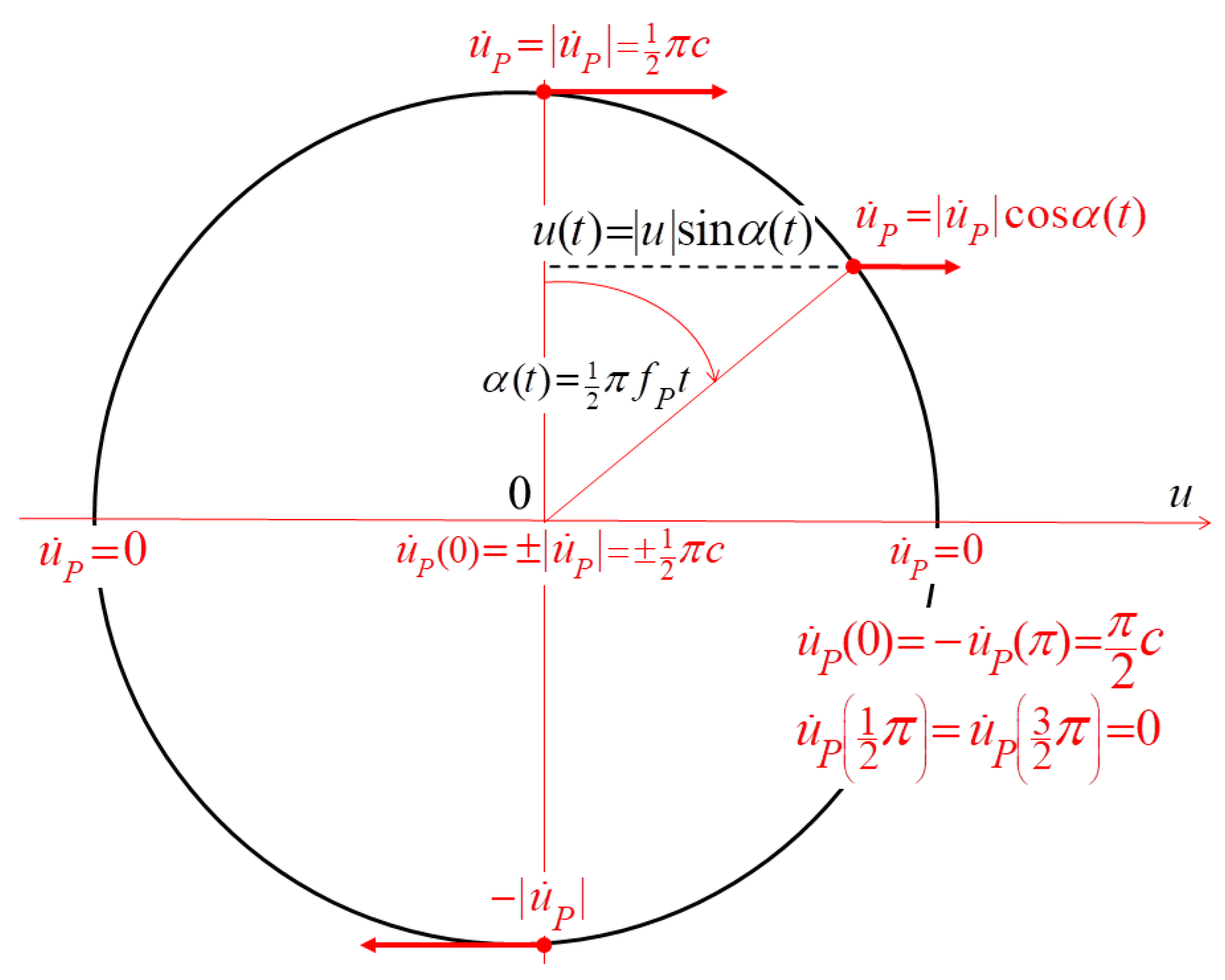
5.4. The Time Dependence of Irrotational Deformation, ${\sigma }_0\left(t,x\right)$

In this section, we combine the equations of the mass continuity, CE, and of the state to obtain the time dependence of the scalar potential ${\sigma }_0$ (compression) in an ideal elastic solid (it can be considered an quaternionic equivalent of the Riccati equation that usually is written as follows: $\left(\mathsf{\partial }/\mathsf{\partial }t+\dot{u}\cdot \nabla \right)\sigma +\sigma \circ \sigma +{\sigma }_p=0$). Obviously, a simplified assumption of the constant Planck density is disobeyed (consequently, all the waves’ velocities depend on the displacement). The mass density in an ideal elastic solid in ${ℝ}^3$ is affected only by displacements u:

$$\frac{\mathsf{\partial }{\rho }_P}{\mathsf{\partial }t}+{\rho }_P\mathrm{div}\dot{u}=-\dot{u}\cdot \mathrm{grad}{\rho }_P.$$

(82)

The mass density can be defined as follows:

$${\rho }_P\left(t,x\right)=\underset{\mathsf{\Omega }\to 0}{\lim }m \left(\mathsf{\Omega }\right)/\mathsf{\Omega } \left(t,x\right),$$

(83)

where $m \left(\mathsf{\Omega }\right)$ denotes the time-invariant mass contained in the deformed volume $\mathsf{\Omega } \left(t,x\right)$.

In an ideal elastic medium, it depends exclusively on the irrotational deformation $\left(\mathrm{div}u=\mathrm{div}{u}_0={\sigma }_0\right)$. One can relate the deformation and density in a case of sphere in an ideal elastic continuum. In such a case, the mass in a sphere does not depend on its radius, $m\left(\mathsf{\Omega }\left[r\left(t,x\right)\right]\right)=m=const$, and the density is affected only by the radius:

$${\rho }_P \left(t,x\right)=m /\left(\frac{4}{3}\pi {\left[r \left(t,x\right)\right]}^3\right)\hspace{1em}\Rightarrow \hspace{1em}\mathrm{d}{\rho }_P=-m/\left(\frac{4}{3}\pi r^3\right)3\frac{\mathrm{d}r}{r}=-3{\rho }_P\frac{\mathrm{d}r}{r}.$$

(84)

In an ideal elastic continuum, $\mathrm{d}{\sigma }_0=\mathrm{d}r/r$ and (85) in quaternionic notation becomes the following:

$$\frac{1}{{\rho }_P}\mathrm{d}{\rho }_P=-3\hspace{0.33em}\mathrm{d}{\sigma }_0.$$

(85)

Consequently, from (86), it follows:

$$\frac{1}{{\rho }_P}\frac{\mathsf{\partial }{\rho }_P}{\mathsf{\partial }t}=-3\frac{\mathsf{\partial }{\sigma }_0}{\mathsf{\partial }t} \mathrm{and} \frac{1}{{\rho }_P}\mathrm{grad}{\rho }_P=-3\mathrm{grad}{\sigma }_0.$$

(86)

By introducing relations (87) and the identity $\mathrm{div}\dot{u}=\frac{\mathsf{\partial }}{\mathsf{\partial }t}\mathrm{div}{u}_0=\frac{\mathsf{\partial }{\sigma }_0}{\mathsf{\partial }t}$ into the Equation (83), we obtain the following:

$$-3\frac{\mathsf{\partial }{\sigma }_0}{\mathsf{\partial }t}+\frac{\mathsf{\partial }{\sigma }_0}{\mathsf{\partial }t}=3\dot{u}\cdot \mathrm{grad}{\sigma }_0,$$

(87)

by expressing the velocity as a function of the Cauchy–Riemann derivative, i.e., introducing (43), we finally obtain the following:

$$\frac{\mathsf{\partial }{\sigma }_0}{\mathsf{\partial }t}=\frac{3}{2}\frac{\hslash }{m}\left(\mathrm{D}\sigma \right)\cdot \mathrm{grad}{\sigma }_0=\frac{3}{2}\frac{\hslash }{m}\left(\mathrm{rot}\widehat{\varphi }+\mathrm{grad}{\sigma }_0\right)\cdot \mathrm{grad}{\sigma }_0.$$

(88)

The quaternion form of the first-order wave equation presented in this work allows one to obtain an insight into the Dirac equation and therefore spin ½. Spin ½ fermions are the cause of the Pauli exclusion principle, and therefore it is important to understand the physical meaning of spin ½ in the Planck–Kleinert model. In order to visualize this concept, a simple interactive simulation of a periodically twisting and compressing 3D grid illustrating spin ½ in an elastic solid for two particles is presented [68,69].

6. Conclusions

The presented quaternion representation of quantum mechanics allows its ontological interpretation. In simple words, the correspondence between classical and quaternion quantum equations permits one to consider the universe (vacuum) as an ideal elastic solid. Elementary particles would have to be standing or soliton-like waves. Tension induced by the compression and twisting of the elastic medium would increase energy density and consequently, carry out the following:

-

generate a gravity forcing;

-

affect the wave speed. Consequently, the gravity could be described by an index of refraction [69].

The present theory was created by combining the Cauchy model of the elastic continuum with the Planck–Kleinert crystal hypothesis. The quaternion–imaginary Lagrangian, the quaternion motion equation, and the quaternionic oscillator allowed the following to be derived:

-

A Schrödinger equation from the functional integral, which identifies the quaternion–imaginary quantum Hamiltonian;

-

The second-order wave equation system describing both the bosons and the gravity in terms of quaternionic Poisson equation;

-

The first-order quaternionic wave equation system;

-

The family of the second-order wave equation systems describing both the particles and the generated quaternionic force fields (four-potential);

-

The Planck constants, $\hslash = m_P c^2 t_P=1.0545727\times {10}^{-34}$, and gravity constant, $G=l_P^3/\left(t_P^2{m}_P\right)=6.674082\times {10}^{-11}$;

-

The quaternionic continuity equation in an ideal elastic solid.

The meaning of the particle mass center (particle ≡ wave) is assigned here to “space-localized” and is used in the sense given by the Bodurov definition [70].

Quaternion quantum mechanics has many new features that make it a much richer theory. Its great potential is visible, e.g., in the following:

-

The comparison of the first-order wave equations in quaternion formulation, Equation (81), with the form in the Dirac algebra formalism:

$$\begin{array}{l}\mathrm{Dirac}: \left(i {\gamma }^{\mu }{\mathsf{\partial }}_{\mu }-\frac{mc}{\hslash }\right)\psi \left(t,x\right)=0 \mathrm{where} {\gamma }^{\mu }{\mathsf{\partial }}_{\mu }=\frac{1}{c}\frac{\mathsf{\partial }}{\mathsf{\partial }t}+{\alpha }_1\frac{\mathsf{\partial }}{\mathsf{\partial }x}+{\alpha }_2\frac{\mathsf{\partial }}{\mathsf{\partial }y}+{\alpha }_3\frac{\mathsf{\partial }}{\mathsf{\partial }z},\\ \mathrm{Quaternion}: {\mathsf{\partial }}_{\widehat{\mu }}\psi \left(t,x\right)-\frac{mc }{\hslash }\beta {\psi }^{*}\cdot \psi \left(t,x\right)=0, \mathrm{where} {\mathsf{\partial }}_{\widehat{\mu }}=\frac{1}{c}\frac{\mathsf{\partial } }{\mathsf{\partial } t}-\mathrm{grad} -\mathrm{rot}\\ \hspace{1em}\hspace{1em}\hspace{1em}\hspace{1em} \mathrm{and} \beta =8\pi m_P/m\sqrt{m/{\rho }_P}\end{array}$$

(89)

-

A simple interactive simulation of a periodically twisting and compressing 3D grid illustrating spin ½ in an elastic solid for two particles is presented [68].

References

1. Danielewski, M.; Sapa, L. Foundations of the quaternion quantum mechanics. Entropy 2020, 22, 1424. [Google Scholar] [CrossRef] [PubMed]
2. Schrödinger, E. The Interpretation of Quantum Physics; Ox Bow Press: Woodbridge, CN, USA, 1995. [Google Scholar]
3. Bohm, D.A. Suggested interpretation of the quantum theory in terms of hidden variables. I and II. Phys. Rev. 1952, 85, 166–193. [Google Scholar] [CrossRef]
4. Bohm, D.; Hiley, B.J. The Undivided Universe: An Ontological Interpretation of Quantum Theory; Routledge: Philadelphia, PA, USA, 1993; p. 397. [Google Scholar]
5. Chen, P.; Kleinert, H. Deficiencies of Bohm trajectories in view of basic quantum principles. Electr. J. Theor. Phys. 2016, 13, 1–12. [Google Scholar]
6. Bell, J.S. On the Einstein Podolsky Rosen paradox. Physics 1964, 1, 195–200. [Google Scholar] [CrossRef]
7. Bell, J.S. Schrödinger–Centenary Celebration of a Polymath; Kilmister, C.W., Ed.; Cambridge University Press: Cambridge, UK, 1987; pp. 41–52. [Google Scholar]
8. Feynman, R.P. The Character of Physical Law, 2nd ed.; The MIT Press: Cambridge, MA, USA, 2017. [Google Scholar]
9. Gell-Mann, M. The Nature of the Physical Universe; Huff, D., Prewett, O., Eds.; John Wiley & Sons: New York, NY, USA, 1979; p. 29. [Google Scholar]
10. Bodurov, T. Solitary waves interacting with an external field. Int. J. Theor. Phys. 1996, 35, 2489–2499. [Google Scholar] [CrossRef]
11. Bodurov, T. Derivation of the nonlinear Schrödinger equation from first principles. Ann. Fond. Louis Broglie 2005, 30, 343–352. [Google Scholar]
12. Białynicki-Birula, I.; Mycielski, I.J. Nonlinear wave mechanics. Ann. Phys. 1976, 100, 62–93. [Google Scholar] [CrossRef]
13. Weng, Z.-H. Field equations in the complex quaternion spaces. Adv. Math. Phys. 2014, 2014, 450262. [Google Scholar] [CrossRef]
14. Horodecki, R. De Broglie wave and its dual wave. Phys. Lett. 1981, 87A, 95–97. [Google Scholar] [CrossRef]
15. Horodecki, R. Superluminal singular dual wave. Lett. Novo C. 1983, 36, 509–511. [Google Scholar] [CrossRef]
16. Close, R. Torsion waves in three dimensions: Quantum mechanics with a twist. Found. Phys. Lett. 2002, 15, 71–83. [Google Scholar] [CrossRef]
17. Close, R.A. Exact description of rotational waves in an elastic solid. Adv. Appl. Clifford Algebras 2011, 21, 73–281. [Google Scholar] [CrossRef]
18. Close, R.A. Spin angular momentum and the dirac equation. EJTP 2015, 12, 43. [Google Scholar]
19. Birkhoff, G.; von Neumann, J. The logic of quantum mechanics. Ann. Math. 1936, 37, 823–843. [Google Scholar] [CrossRef]
20. Yang, C.N. High energy nuclear physics. In Proceedings of the Seventh Annual Rochester Conference, Rochester, NY, USA, 15–19 April 1957; Midwestern Universities Research Association, Interscience Publishing, Inc.: New York, NY, USA, 1957; pp. 9–26. [Google Scholar]
21. Finkelstein, D.; Jauch, J.M.; Schiminovich, S.; Speiser, D. Foundations of quaternion quantum mechanics. J. Math. Phys. 1962, 3, 207–220. [Google Scholar] [CrossRef]
22. Brumby, S.P.; Joshi, G.C. Global effects in quaternionic quantum field theory. Found. Phys. 1996, 26, 1591–1599. [Google Scholar] [CrossRef]
23. Brumby, S.P.; Joshi, G.C. Experimental status of quaternionic quantum mechanics. Chaos Solitons Fract. 1996, 7, 747–752. [Google Scholar] [CrossRef]
24. Adler, S.L. Quaternionic quantum field theory. Phys. Rev. Let. 1985, 55, 783–786. [Google Scholar] [CrossRef]
25. Adler, S.L. Mechanics and Quantum Fields; Oxford University Press: New York, NY, USA, 1995. [Google Scholar]
26. Adler, S.L. Quantum Theory as an Emergent Phenomenon; Cambridge University Press: Cambridge, UK, 2004. [Google Scholar]
27. Nottale, L. Origin of complex and quaternionic wavefunctions in quantum mechanics: The scale-relativistic view. Adv. Appl. Clifford Algebr. 2008, 18, 917–944. [Google Scholar] [CrossRef]
28. Gantner, J. On the equivalence of complex and quaternionic quantum mechanics. Quantum Stud. Math. Found. 2018, 5, 357–390. [Google Scholar] [CrossRef]
29. Danielewski, M.; Sapa, L. Nonlinear Klein–Gordon equation in Cauchy–Navier elastic solid. Cherkasy Univ. Bull. Phys. Math. Sci. 2017, 1, 22–29. [Google Scholar]
30. Whittaker, E. A History of the Theories of Aether and Electricity; Philosophical Library: New York, NY, USA, 1951; Volume 1. [Google Scholar]
31. Cauchy, A.L. De la pression ou tension dans un corps solide. Exerc. Math. 1827, 2, 60–81. [Google Scholar]
32. Maxwell, J.C. A Dynamical theory of the electromagnetic field. Phil. Trans. R. Soc. Lond. 1865, 155, 459–512. [Google Scholar] [CrossRef]
33. Maxwell, J.C. Introductory lecture on experimental physics. In The Scientific Papers of James Clerk Maxwell; Niven, W.D., Ed.; Dover: New York, NY, USA, 1965; Volume II, pp. 241–255. [Google Scholar]
34. Kleinert, H. Gravity as theory of defects in a crystal with only second–gradient elasticity. Ann. Phys. 1987, 44, 117–119. [Google Scholar] [CrossRef]
35. Kleinert, H. Emerging gravity from defects in world crystal. Braz. J. Phys. 2005, 35, 359–361. [Google Scholar] [CrossRef]
36. Deb, S.; Das, S.; Vagenas, E.C. Discreteness of space from GUP in a weak gravitational field. Phys. Lett. B 2016, 755, 17–23. [Google Scholar] [CrossRef]
37. Ali, A.F.; Das, S.; Vagenas, E.C. Discreteness of space from the generalized uncertainty principle. Phys. Lett. B 2009, 678, 497–499. [Google Scholar] [CrossRef]
38. Danielewski, M. The Planck–Kleinert crystal. Z. Naturforsch. 2007, 62, 564–568. [Google Scholar] [CrossRef]
39. Danielewski, M.; Sapa, L. Diffusion in Cauchy elastic solid. Diff. Fundam. 2020, 33, 1–14. [Google Scholar]
40. Lanczos, C. Die Funktionentheoretischen Beziehungen der Maxwellschen Æthergleichungen-Ein Beitrag zur Relativitäts und Elektronentheorie. In C. Lanczos Collected Published Papers with Commentaries; Davis, W.R., Chu, M.T., Dolan, P., McCornell, J.R., Norris, L.K., Ortiz, E., Plemmons, R.J., Ridgeway, D., Scaife, B.K.P., Stewart, W.J., et al., Eds.; North Carolina State University: Raleigh, CA, USA, 1998; Volume VI, pp. A1–A82. [Google Scholar]
41. Lanczos, C. Die tensoranalytischen Beziehungen der Diracschen Gleichung (The tensor analytical relationships of Dirac’s equation). Z. Phys. 1929, 57, 447–473. [Google Scholar] [CrossRef]
42. Lanczos, C. Zur kovarianten Formulierung der Diracschen Gleichung (On the covariant formulation of Dirac’s equation). Z. Phys. 1929, 57, 474–483. [Google Scholar] [CrossRef]
43. Lanczos, C. Die Wellenmechanik als Hamiltonsche Dynamik des Funktionraumes. Eine neue Ableitung der Dirak-schengleichung (Wave mechanics as Hamiltonian dynamics of function space. A new derivation of Dirac’s equation). Z. Phys. 1933, 81, 703–732. [Google Scholar] [CrossRef]
44. Lanczos, C. Electricity as a natural property of Riemanian geometry. Phys. Rev. 1932, 39, 716–736. [Google Scholar] [CrossRef]
45. Silvis, M.H. A Quaternion Formulation of the Dirac Equation; Report; Centre for Theoretical Physics, University of Groningen: Groningen, The Netherlands, 2010. [Google Scholar]
46. Graves, R.P. Life of Sir William Rowan Hamilton; Hodges, Figgis, & Co.: Dublin, Ireland, 1989. [Google Scholar]
47. Maxwell, J.C. Remarks on the mathematical classification of physical quantities. Proc. Lond. Math. Soc. 1869, 3, 224–233. [Google Scholar] [CrossRef]
48. Gürlebeck, K.; Sprössig, W. Quaternionic and Clifford Calculus for Physicists and Engineers; Mathematical Methods in Practice; Wiley: New York, NY, USA, 1997; ISBN 0-471-96200-7. [Google Scholar]
49. Altmann, S.L. Rotations, Quaternions, and Double Groups; Clarendon Press: New York, NY, USA, 1986; ISBN 0-19-855372-2. [Google Scholar]
50. Dorst, L.; Fontijne, D.; Mann, S. Geometric Algebra for Computer Science; Elsevier: Amsterdam, The Netherlands, 2007. [Google Scholar] [CrossRef]
51. Gürlebeck, K.; Sprößig, W. Quaternionic Analysis and Elliptic Boundary Value Problems; Akademie-Verlag: Berlin, Germany, 1989. [Google Scholar]
52. Cauchy, A.L. Récherches sur l’équilibre et le movement intérieur des corps solides ou fluides, élastiques ou non élastiques. Bull. Sot. Philomath. 1823, 9, 300–304. [Google Scholar]
53. Todhunter, I. A History of the Theory of Elasticity and of the Strength of Materials; Pearson, K., Ed.; Cambridge University Press: Cambridge, UK, 2014. [Google Scholar] [CrossRef]
54. Poisson, D. Mémoire sur l’équilibre et le mouvement des corps élastiques. Mém. Acad. Sci. Paris 1829, 8, 357–570. [Google Scholar]
55. Neumann, F. Vorlesungen Über die Theorie der Elasticität der Festen Körper und des Lichtäthers; B.G. Teubner: Leipzig, Germany, 1885. [Google Scholar]
56. Duhem, P. Sur l’intégrale des équations des petits mouvements d’un solide isotrope. Mém. Soc. Sci. Bordeaux Ser. V 1898, 3, 316. [Google Scholar]
57. Love, A.E.H. Mathematical Theory of Elasticity, 4th ed.; Dover Publications Inc.: New York, NY, USA, 1944; p. 8. [Google Scholar]
58. Landau, L.D.; Lifshitz, E.M. Theory of Elasticity, 3rd ed.; Butterworth-Heinemann Elsevier Ltd.: Amsterdam, The Netherlands, 1986. [Google Scholar]
59. Helmholtz, H.V. Über integrale der hydrodynamischen Gleichungen, welche den Wirbel-bewegungen entsprechen. Crelle J. 1858, 55, 25–55. [Google Scholar]
60. National Institute of Standards and Technology. Available online: http://physics.nist.gov (accessed on 10 November 2018).
61. Weinberg, S. The Quantum Theory of Fields; Cambridge University Press: Cambridge, UK, 1995; Volume 1, pp. 7–8. [Google Scholar]
62. Ulrych, S. Higher spin quaternion waves in the Klein-Gordon theory. Int. J. Theor. Phys. 2013, 52, 279–292. [Google Scholar] [CrossRef]
63. Zeidler, E. Nonlinear Functional Analysis and Its Applications II/A: Linear Monotone Operators; Springer: New York, NY, USA, 1990; p. 18. [Google Scholar]
64. Hays, J. Tracing the History of Clifford Algebra. Available online: https://web.archive.org/web/20040810155540/jonhays/clifhistory.htm (accessed on 15 February 2021).
65. Dirac, P.A.M. The quantum theory of the electron. Proc. R. Soc. Lond. A 1928, 117, 610. [Google Scholar]
66. Dirac, P.A.M. Is there an aether? Nature 1952, 169, 702. [Google Scholar] [CrossRef]
67. Snoswell, M. Personal communications, 2022.
68. Roth, C. Simulation of Electron Spin. Available online: https://elastic-universe.org/ (accessed on 15 August 2023).
69. Evans, J.; Alsing, P.M.; Giorgetti, S.; Nandi, K.K. Matter waves in a gravitational field: An index of refraction for massive particles in general relativity. Am. J. Phys. 2001, 69, 1103–1110. [Google Scholar] [CrossRef]
70. Bodurov, T. Generalized Ehrenfest theorem for nonlinear Schrödinger equations. Int. J. Theor. Phys. 1988, 37, 1299–1306. [Google Scholar] [CrossRef]
Figure 1. The Planck cycle. The velocity of the displacement in the Planck volume of the ideal elastic continuum visualized as 1 projection of the circular motion: u ˙ P ( t ) = u ˙ P α ( t ) = u ˙ P cos α ( t ) , where α ( t ) = 1 2 π f P   t and u ˙ P = 1 2 π c is the magnitude of the displacement rate, according to Equation (56).
Symmetry 15 01672 g001