1. Introduction
Considering the complexity and imprecision inherent in many real-world situations, decision-makers (DMs) often find it more beneficial to express their preferences using linguistic terms, like “good” quality or “very bad” credit scores, instead of specific numerical figures [
1].
The fuzzy linguistic approach, introduced by Zadeh [
2], revolutionized the representation of assessment values by using linguistic terms. However, this approach, which restricts a linguistic variable’s value to a single linguistic term, may not fully capture the preferences of DMs. Indeed, due to the complexity of DMs’ cognition, they may be hesitant among various linguistic terms, necessitating a richer linguistic expression to better convey their preferences.
In response to these limitations, numerous researchers have proposed a variety of expression models, as detailed in
Table 1. Notably, Rodriguez et al. [
3] initiated the use of hesitant fuzzy linguistic term sets (HFLTSs) that incorporate ordered and consecutive linguistic terms to represent linguistic variables, providing a more nuanced alternative to employing a single exact linguistic term. Due to their innovative and effective approach to expressing qualitative judgments by DMs, HFLTSs have attracted considerable scholarly attention in the realms of operational laws [
4,
5,
6], aggregation operators [
7,
8], measures of distance and similarity [
9,
10,
11], and various ranking approaches [
12,
13].
Nonetheless, HFLTSs inherently consider the degree of membership of an element to be one, while overlooking the degree of non-membership and hesitancy. This could pose significant challenges in real-world decision-making scenarios where preference information is commonly ambiguous, unreliable, or inadequate, making the consideration of non-membership and hesitancy degrees crucial. For instance, an evaluation such as “the market prospect of the new product ranges from medium to high and it cannot be bad” cannot be adequately reflected using HFLTSs.
To address this limitation, Beg and Rashid [
14] proposed hesitant intuitionistic fuzzy linguistic term sets (HIFLTSs), which introduced a non-membership degree to each linguistic element. HIFLTSs allow DMs to express their uncertainty in a more nuanced and granular manner, capturing not only the degree of membership but also the degree of non-membership and hesitation. This enables a more comprehensive representation of DMs’ preferences and uncertainties, leading to more accurate decision-making processes. Consequently, research on HIFLTSs has attracted extensive attention from scholars and has achieved numerous advancements. For instance, Liu et al. [
15] developed hesitant intuitionistic fuzzy uncertain linguistic sets, allowing an uncertain linguistic term to have sets of intuitionistic fuzzy numbers. Zhou et al. [
16] proposed intuitionistic hesitant linguistic sets (IHLSs) based on HIFLTSs, defining basic operations and aggregation operators for MCDM problems. Similarly, Faizi et al. [
17] introduced a novel outranking method for MAGDM in the HIFLTSs environment. Liu et al. [
18] advanced the distance measure of HIFLTSs based on mean-standard deviation for resolving MADM problems. Faizi et al. [
19] proposed several distance measures for HIFLTSs based on a risk factor parameter.
Table 1.
Survey of related research works.
Table 1.
Survey of related research works.
| Methods | Expression
Model | Type | Does It Consider the Membership and Non-membership Degree Simultaneously | Evaluation Item |
|---|
| Method in [2] | fuzzy linguistic approach (FLA) | Qualitative | No | Single linguistic term |
| Method in [3] | hesitant fuzzy linguistic term sets (HFLTSs) | Qualitative | No | Multiple linguistic terms |
| Method in [14] | hesitant intuitionistic fuzzy linguistic term sets (HIFLTSs) | Qualitative | Yes | Multiple linguistic terms |
| Method in [20] | intuitionistic fuzzy sets (IFS) | Quantitative | Yes | Single numerical value |
| Method in [21] | hesitant fuzzy sets (HFSs) | Quantitative | No | Multiple numerical values |
| Method in [22] | linguistic intuitionistic fuzzy number (LIFN) | Qualitative | Yes | Single linguistic term |
| Method in [23] | intuitionistic hesitant
fuzzy linguistic term sets (IHFLTSs) | Qualitative | Yes | Single linguistic term |
| Method in [24] | interval-valued intuitionistic hesitant fuzzy
sets (IVIHFSs) | Qualitative | Yes | Multiple linguistic terms |
The aforementioned literature validates the potential of HIFLTSs, making it a promising research field with both theoretical and practical applications. However, certain limitations still exist:
- (1)
The flexibility and complexity offered by HIFLTSs are double-edged swords. To date, only Zhang et al. [
15] have presented fundamental operations based directly on the subscript of linguistic terms. However, these operations encounter a critical limitation in certain situations where an “exceed the bound” issue arises. For instance, let
be a linguistic term set,
is a positive real number, and
and
be two HIFLEs, then, by using the operational laws of HIFLTSs given by [
15], we can obtain
and
, which exceed the upper bound
s6. Moreover, multiplication and division operations based directly on the subscripts of linguistic terms seem illogical.
- (2)
Current score functions and accuracy functions in HIFLTSs may not incorporate the hesitancy degree, which is an essential piece of information for decision-making. Consequently, intuitive conflicts could arise in certain scenarios. For example, a DM providing a “good” assessment for the membership degree exhibits no hesitancy, while an evaluation of “between medium and very good” conveys a certain degree of hesitancy. Evidently, the reliability of the first linguistic assessment should be superior to that of the second, implying that the latter should be ranked lower. However, existing methodologies treat these two elements as equals, which is a perspective that contradicts our understanding.
- (3)
When comparing with established ranking methodologies such as the TOPSIS [
25], VIKOR [
5], SMART [
26], and MOORA [
27], the multiplicative multi-objective optimization by ratio analysis (MULTIMOORA) method stands out with its time efficiency, robustness, simplicity, and effectiveness [
28,
29,
30]. This method is distinguished by its three unique aggregation models that separately address fully compensatory, non-compensatory, and incompletely compensatory aspects. Despite its advantages, current research indicates that the MULTIMOORA method has yet to be implemented within the HIFLTSs environment for MAGDM problems.
Motivated by the above analysis, this study proposes a novel method for addressing MAGDM problems within the HIFLTSs environment. Specifically, the following three areas are the main focus of this paper:
- (1)
A series of innovative basic operational laws for HIFLTSs aimed at enhancing their applicability and streamlining their methodological approach in the context of MAGDM models are introduced.
- (2)
This paper presents a new score function and accuracy function for HIFLTSs, considering the degree of hesitancy. Moreover, in an effort to further expand the theoretical framework of HIFLTSs, this study establishes correlation measures and correlation coefficients for HIFLTSs.
- (3)
This paper introduces a MAGDM model rooted in the MULTIMOORA approach. This model employs the proposed score function and correlation measures in the HIFLTS context.
This paper is structured as follows:
Section 2 provides a concise review of basic definitions and operations pertaining to HIFLTSs, intuitionistic fuzzy sets (IFSs), correlation measures, and coefficients.
Section 3 delves into the innovative basic operational laws for HIFLTSs.
Section 4 proposes a novel score function and accuracy function for HIFLTSs. In
Section 5, the correlation measures and correlation coefficients of HIFLTSs are presented. The MAGDM method, which is based on the MULTIMOORA approach, is introduced in
Section 6. A real-world case study is presented in
Section 7.
Section 8 provides a comparative analysis with some existing related methodologies. Our conclusions are drawn in
Section 9.
2. Preliminaries
This section presents the fundamental definitions and procedures concerning hesitant intuitionistic fuzzy linguistic term sets, intuitionistic fuzzy sets, measures of correlation, correlation coefficients, and the linguistic scale function.
2.1. HIFLTSs
Definition 1. [14] Let be a universe of discourse and be a consecutive linguistic term set. As a hesitant intuitionistic fuzzy linguistic term set on X, Es is in mathematical terms ofwhere and are subsets of the consecutive linguistic term set S and can be expressed as and , and represent the numbers of linguistic terms in and .
and denote the membership and non-membership degree of a linguistic variable to the linguistic term set S. For each HIFLTS with Es on X, the following conditions should be satisfied: For convenience, is called the hesitant intuitionistic fuzzy linguistic element (HIFLE).
Definition 2. [17] Let
represent an LTS.
denotes an HIFLE, with
and
expressing the numbers of linguistic terms in
and
, respectively. Then, the score function and accuracy function of
can be defined as follows: where
,
,
, and
.
Theorem 1. [17] Let represent an LTS. and denote two HIFLEs. Then,
- (1)
If
, then ;
- (2)
If , then
- i
If , then
- ii
If , then
2.2. IFSs
The fundamental principle of intuitionistic fuzziness is entrenched in many existing models. Its assumption that non-membership should be evaluated separately from membership has evolved to very general models [
20]. Atanassov pioneered the utilization of “orthopairs”, whereby a pair of values in the unit interval provide the support for and against membership of an element to the “orthopair fuzzy set”. Based on this idea, the concept of IFSs is formulated as follows:
Definition 3. [31,32] Let X be a non-empty universe of discourse and an IFSs’ A in X is given by , where
and
, with the condition
for all
. The numbers of
and
denote the degree of membership and non-membership of
to the set A, respectively. In addition,
is termed as the hesitancy degree of x to the set A and
for all
.
Definition 4. [33] Let and denote two intuitionistic fuzzy pairs (IFPs), and is a positive real number. Then,
- (1)
- (2)
- (3)
- (4)
- (5)
2.3. Linguistic Scale Function
The principles of the linguistic scale function (LSF) can be applied to various forms of the semantics of linguistic terms. Typically, the LSF
f is a function that increases monotonically, where
;
, and
. In accordance with the diverse semantic distributions signified by linguistic terms, [
33] identified three distinct types of LSF.
- (1)
If the linguistic semantics are equally divided, the LSF is defined as follows:
- (2)
If the linguistic semantics of any neighboring linguistic terms are unequally divided, the variance value appears to increase on either side of
, and the LSF is defined as follows:
If the scale level is , then .
- (3)
If the linguistic semantics of any neighboring linguistic terms are unequally divided, the variance value appears to decrease on either side of
, and the LSF is defined as follows:
2.4. Correlation Measures and Coefficients
Correlation measures can be regarded as the degree of closeness between two variables in a linear relationship, and various types of correlation coefficients have been proposed in the context of fuzzy decision-making problems. These include entropy weights-based correlation coefficients [
34], correlation coefficients of interval-valued intuitionistic fuzzy sets [
35], correlation coefficients of hesitant fuzzy sets [
36], correlation coefficients of dual hesitant fuzzy linguistic term sets [
37], among others.
With regards to intuitionistic fuzzy sets, they can be categorized into two types: correlation measures derived from a statistical perspective and those based on information energy. Dimitrescu [
38] proposed one of the fundamental definitions of informational energy in fuzzy sets, laying the groundwork for subsequent extensions and applications. Ejegwa et al. [
39] have conducted extensive research on correlation coefficients of intuitionistic fuzzy sets and their real-world applications. Szmidt et al. [
21] proposed a novel method for the ranking of alternatives represented as intuitionistic fuzzy sets. Hung et al. [
40] presented the correlation measure based on the perspective of statistics that took the degree of membership and non-membership as two fuzzy sets, respectively. Mitchell et al. [
41] took account of the hesitancy degree and proposed a new formula for measuring the correlation of IFSs. Szmidt et al. [
42] introduced an extended method of correlation measures that considered the IFSs to be the common membership function ensembles. All these correlation measure methods draw inspiration from classical statistics, with the resultant values falling within the unit interval [0, 1]. From an information energy perspective, Gerstenkorn et al. [
43] proposed a novel form of correlation measure for IFSs, which is defined as:
Definition 5. [40] Let X be a non-empty universe of discourse,
and are two IFSs, then the correlation coefficient based on the information energy is defined as follows: Furthermore, Huang et al. [
44] introduced the definition of centroid method-based correlation measures for IFSs. Xu et al. [
45] developed a novel form of correlation measure that allows the correlation coefficients of any two IFSs to be equivalent if and only if they are the same. As these correlation measures are based on information energy, the derived correlation coefficients belong to the interval [0, 1].
3. The Novel Basic Operational Laws for HIFLTSs
As aforementioned, the current operational laws for HIFLTSs exhibit significant limitations under certain circumstances. Let us illustrate this with a specific example.
Example 1. Let be an LTS, and be two HIFLEs, and .
Then, based on the existing operations proposed in Ref. [15], we can derive that and .
Obviously, the results exceed the upper bound s6.
Hence, it is imperative to define novel basic operational laws for HIFLTSs to address the above limitations. Inspired by Refs. [
32,
46], the linguistic scale functions
f and
f−1 can be regarded as transformation tools, enabling equivalent transformations between HIFLEs and IFSs. In other words, based on the equivalent transform function
f, HIFLEs can be converted into IFSs, and the basic operations of IFSs (Definition 4) can be used to calculate these transformed HIFLEs. Subsequently, the inverse function
f−1 can be applied to equivalently transform these calculation results back to HIFLEs. As a result, we can develop the following novel basic operational laws for HIFLEs:
Definition 6. Let represent an LTS.
and denote two HIFLEs, with , and expressing the numbers of linguistic terms in , and , respectively. f and f−1 denote the equivalent transformation functions of HIFLEs and IFSs, and is a positive real number. Then,
- (1)
;
- (2)
;
- (3)
;
- (4)
.
Theorem 2. Let represent an LTS.
and denote two HIFLEs, and ,
, and are three positive real numbers. Then,
- (1)
;
- (2)
;
- (3)
;
- (4)
.
Proof. (1) and (2) are obvious, and we can omit the proofs of them.
- (3)
- (4)
□
Next, we will proceed to analyze the proposed basic operational laws using the values provided in Example 1. For convenience, the first type of LSF is chosen as the equivalent transformation function. Using this, we can obtain , , , and . Moreover, the final results can be calculated based on Definition 6 as:
- (1)
- (2)
- (3)
- (4)
4. A Novel Score Function and Accuracy Function of HIFLTSs Considering the Hesitancy Degree
HIFLTSs enable the evaluation of membership and non-membership degrees using more than one linguistic term, providing richer linguistic expressions and a greater level of uncertainty and hesitancy. For instance, when a group of DMs are seeking to elucidate the manufacturing plan for a new project, a DM who assigns the linguistic evaluation “good” to the membership degree shows no sign of hesitancy. Conversely, a DM who rates the membership degree as “between medium and very good” demonstrates a certain degree of hesitancy. It is evident that the hesitancy level of the latter evaluation should exceed that of the former, suggesting that the reliability of the second evaluation should be less than that of the first. However, the relationship between these two evaluations is marked as equal according to the current score function and accuracy function, which conflicts with our perception. Consequently, it seems reasonable to incorporate the hesitancy degree when defining the score function for HIFLTSs.
The concept of hesitancy degree was first introduced by Liao et al. [
36] in their exploration of the correlation among hesitant fuzzy sets. Subsequently, Wei et al. [
47] presented a method to measure the degree of hesitancy, which is dependent on the deviation among linguistic terms. Ref. [
12] developed a comprehensive method to evaluate the hesitancy degree of a HFLE based on the count of linguistic terms. Considering that the DMs are more sensitive to a large number of linguistic terms than to a few, it is indicated that the function of the hesitancy degree is non-linear and should satisfy
. Thus, we adopt the hesitant degree function for our analysis, which is defined as
where
and
represent the number of linguistic terms in
and
. Based on the hesitant degree function, we introduce a new score function for HIFLE, which is defined as follows:
Definition 7. Let represent an LTS. denotes an HIFLE, with and expressing the numbers of linguistic terms in and , respectively. The improved score function of can be defined as follows:where and .
Moreover, according to the degree of membership, the score function is a strictly monotonically increasing function and a strictly monotonically decreasing function according to the degree of non-membership. Consequently, the following properties are maintained: Proposition 1. Let represent an LTS. and denote two HIFLEs, with , and expressing the numbers of linguistic terms in , and , respectively.
- (1)
- (2)
If and
, then ; if , then .
- (3)
If , , and , then ; if , then .
Proof. (1) If we have by Equation (7), then , , and . If , that is , then takes the minimum and . If , that is , , takes the maximum and .
(2) Let and , then can be transformed to , , and . Subsequently, take the partial derivative with respect to x and y, we can obtain ; . Thus, is a strictly monotonically increasing function with respect to , and a strictly monotonically decreasing function of . This completes the proof of proposition (2).
(3) , , and , thus and , ; if and , thus and , then . □
Furthermore, from Definition 7 we can find that if , then , and we are unable to make a comparison in this case. Therefore, we propose the accuracy function of to deal with this condition as follows.
Definition 8. Let represent an LTS. denotes an HIFLE, with and expressing the numbers of linguistic terms in and , respectively. The improved accuracy function of can be defined as: Theorem 3. Let be an LTS. and denote two HIFLEs. Then
If , then ;
If , then ;
If , and
- (1)
If , then ;
- (2)
If , then .
Example 2. Let be an LTS. There are four HIFLEs: Based on the Definition 2, we can obtain
and it shows that
.
However, by utilizing the above defined score function and accuracy function, we can calculate , , , and . The results indicate that , which aligns with our cognitive understanding.
5. The Correlation Measures and Correlation Coefficients of HIFLTSs
In this section, we will explore the correlation measures and coefficients between two HIFLTSs. As previously discussed, there are two paradigms for dealing with correlation measures: the classical statistics approach and the information energy-based approach. The former relies heavily on a substantial volume of samples. However, within the context of MAGDM involving HIFLTSs, we frequently operate with a finite and relatively limited set of HIFLTSs. Consequently, we derive the correlation measure from an information energy-based perspective. Inspired Ref. [
40], we propose the concept of information energy within HIFLTSs, which is defined as follows:
Definition 9. Let represent an LTS. denotes a HIFLTSs. Then, the information energy of can be defined as follows:where represents the cardinality of X, and denote the numbers of linguistic terms in and ,
respectively.
Based on the definition of information energy, we present the concept of correlation between two HIFLTSs and as follows:
Definition 10. Let represent an LTS. and denote two HIFLTSs. Then, the correlation between and can be defined as follows:where and are the maximum of linguistic terms in and ,
.
Therefore, the shorter one should be extended by adding some linguistic terms until and .
Inspired by the method proposed by Refs. [4,10], we increase the relatively shorter and by adding the linguistic terms and where Mmax, Mmin, Nmax, and Nmin are the maximum term and minimal term in the shorter and .
Based on the definitions of correlation and information energy of HIFLTSs, we develop the correlation coefficient between two HIFLTSs and as follows:
Definition 11. Let represent an LTS. For two HIFLTSs and , the correlation coefficient between and can be defined as follows: Proposition 2. Let represent an LTS. For two HIFLTSs and , the following properties of hold:
- (1)
- (2)
- (3)
Proof. (1) and (2) are obvious, and we can omit the proofs of them.
(3) According to the Cauchy inequality,
, where
, we have
then
. Since
and
, we have
, that is,
. This completes the proof of property (2). □
Example 3. Let
,
, and
be two HIFLEs; the correlation coefficient between
and
can be calculated as follows:
First, we calculate the information energy of and based on Definition 9. Subsequently, we extend the linguistic terms in and according to the rules; it follows that and , and the correlation between and is yielded: .
Finally, the correlation coefficient between and is derived based on Definition 11: .
6. The MAGDM Method Based on the MULTIMOORA Approach in HIFLTS Context
6.1. The Problem Statement
Here, let , , , and . The MAGDM problems discussed in this paper can be depicted as follows:
Let
be a discrete set of
feasible alternatives,
be a finite set of attributes, and
be a group of DMs; the individual decision matrix associated with DM
is as follows:
where
represents the evaluation value of HIFLEs associated with the criteria
in alternative
given by DM
.
6.2. Determining the Weights of DMs
Numerous efficient methods are available for determining the weights of DMs, which can be classified into two categories: subjective assignment and objective assignment. The former often pose a challenge for DMs to provide precise evaluations in many real-world scenarios. Conversely, the latter assumes that the weight assigned to each DM for different criteria across various alternatives is equal, which may appear somewhat unreasonable. This is because DMs usually come from diverse research areas and may have differences in knowledge structure, evaluation levels, and practical experience. Hence, it seems more reasonable to treat the DMs’ weights concerning different criteria in various alternatives differentially. Consequently, we extend the objective assignment methods and treat the weights of DMs with regard to each distinct attribute in different alternatives differently. Namely, each attribute in the alternative will be assigned a different weight according to the knowledge structure and practical experience of the DM , where and .
Generally, we can determine each DM’s weight depending on their performance. The more similar the preference value is to the mean value, the higher the weight of the DM. Consequently, we can calculate the degree of similarity of
and the mean value
using the correlation coefficient, which is defined as:
where
represents the mean value of the preference value associates with the criteria
in the alternative
.
denotes the degree of similarity between the individual opinions
and the collective opinions associated with the criteria
in the alternative
. Subsequently, the weights of DM
can be determined by the following:
where
,
.
Subsequently, the matrices of
are integrated with the use of the DM’s weights
and we can obtain the collective decision matrix
, where
6.3. Consensus Reaching Process
Considering that DMs frequently come from diverse research fields, possessing distinct knowledge bases, personal inclinations, and hands-on experiences, their respective viewpoints can diverge considerably. As such, the consensus reaching process (CRP) becomes imperative to agree upon the chosen options in MAGDM. This part delves into two pivotal notions used to gauge the similarity between the personal decision matrix and the group decision matrix: the conflict sequence and the group consensus level.
Definition 12 (conflict sequence)
. The conflict sequence is represented as , where each element is characterized as follows:where represents the extent of disagreement between DM and the collective opinions. A higher value of indicates a greater degree of discordance. The DM who displays the highest level of discordance will be asked to modify their opinions in order to enhance the level of group consensus.
Definition 13 (global consensus degree)
. The degree of global consensus can be defined as follows:where ,
represents the correlation coefficient between DMs and , with . A higher value of indicates a greater degree of group consensus.
Moreover, the moderator must define a group consensus threshold based on their judgment. A low value of may lead to the CRP being halted before an acceptable consensus level is attained. On the other hand, an overly high value of could unnecessarily prolong the CRP. In addition, to avoid the discussion being dominated by a minority of DMs and becoming polarized, the parameters of and are employed to set a limit on the number of iterations.
6.4. Determining the Optimal Weights of Attributes
In this section, using the acceptable consistent collective decision matrix R, we determine the optimal weights for attributes
. Here,
and
are assumed to be the sets of benefit attributes and cost attributes, respectively. Initially, we find the positive ideal decision
H+ and the negative ideal decision
H− that correspond to the attribute
as follows:
Using the proposed score function and accuracy function, we can ascertain
and
. Let
and
represent the degree of similarity between the
jth elements of the
ith row in the collective decision matrix R with the positive ideal decision
H+ and the negative ideal decision
H−, respectively. This can be derived as follows:
where
,
,
,
,
.
where
,
,
,
,
.
Next, the LP optimization method must be constructed to identify the optimal weights for the attributes. The objective function of the optimization model aims at minimizing the relative similarity to the
H−, while at the same time maximizing the relative similarity to the
H+.
6.5. The MULTIMOORA Method in the HIFLTSs Environment
In the following section, we present the MULTIMOORA approach for addressing MAGDM issues within the HIFLTS environment. Using Definitions 8 and 9, we are able to determine the score of the collective decision matrix
R as:
First, the vector normalization of
is derived by the following:
After normalization, the decision matrix is generated by all . The MULTIMOORA approach is based on three subordinated methods, which are the ration system (RS), the reference point (RP), and the full multiplicative form (FMF), and use the dominance theory to compute the final ranking.
The HIFLRS model is characterized as the arithmetic weighted aggregation operator. Subsequently, we derive the first subordinate utility value
for the alternative
.
where
denotes the weights of the attribute
.
and
represent the benefit attributes and cost attributes, respectively. By evaluating the utility value
for each alternative, we can rank these alternatives. The higher the value of
, the more preferable the alternative. Once ranked in descending order based on their utility values, we establish the first subordinate ranks of the alternatives, which are denoted as
.
- 2.
Hesitant Intuitionistic Fuzzy Linguistic Reference Point (HIFLRP) model
To avoid the scenario where a chosen alternative underperforms in certain attributes, we introduce the HIFLRP model. This model is shaped by the least performance of alternatives
according to various attributes:
where
if
is a benefit attribute, and
if
is a cost attribute. The alternatives
are ranking by the value of
. The higher the value of
, the more preferable the alternative. Consequently, we establish the second subordinate ranks of the alternatives, denoted as
.
- 3.
Hesitant Intuitionistic Fuzzy Linguistic Full Multiplicative Form (HIFLFMF) model
We can obtain the third subordinate utility value
of the alternative
based on the geometrically weighted aggregation operator.
where
denotes the weights of the attribute
.
and
represent benefit attributes and cost attributes, respectively. The alternatives
are ranking by the value of
in descending order and we obtain the third subordinate ranks of alternatives as
.
To conclude, the three subordinate rankings of alternatives can be collectively combined to produce the ultimate ranking. These can be viewed as three distinct attributes: HIFLRS (
C1), HIFLRP (
C2), and HIFLFMF (
C3). Then, the utility value matrix
and the rank matrix
can be constructed depending on the utility value
and the ranks
associated with each attribute
.
In the conventional MULTIMOORA method, dominance theory was utilized for aggregation. However, as discussed in [
45], this method tends to neglect the unique utility value of every alternative linked with each model and also requires an intricate and lengthy operational procedure. Hence, we use a technique inspired by [
45] to determine the final ranking of alternatives
.
First, we standardize the vector representing the three types of subordinate utility values
and obtain the normalized vector
as follows:
Subsequently, we can transform ordinal values into scores to facilitate the combination of an alternative’s cardinal values. The cardinal value can be perceived as the weight of its associated cardinal value. The ultimate ranking can be determined by sorting the values of
as:
Finally, we summarize the specific processes and describe them in Algorithm 1.
| Algorithm 1 (The proposed MAGDM method) |
Step 1. Collect the individual linguistic assessment values , the given global consensus degree β, maxCycle, and maxInvitations.
Step 2. Determine DMs’ weights using Equations (13) and (14).
Step 3. Construct the collective decision matrix R based on the Definition 6.
Step 4. Calculate the conflict sequence and the global consensus degree using Equations (16) and (17). If , then go to step 6; otherwise, the proceed in the process with step 5.
Step 5. Identify the DM with the greatest degree of discordance, and if he/she has been the DM with the highest degree of discordance for the last maxInvitations, then continue to step 5 for the DM with the next highest degree of discordance, and so on. The DM will be promoted to review his/her judgments; if they remain unchanged, he/she must explain them to the other DMs. Following that, the process returns to step 1, and a new opportunity is provided to each DM to resubmit judgments. It must be emphasized that each DM possesses the right to alter or maintain their opinions.
Step 6. Evaluate various HIFLEs by utilizing the proposed score function and accuracy function, and determine the PIS and NIS corresponding to each attribute .
Step 7. Calculate the and using Equations (20) and (21). Subsequently, determine the optimal weights of each attributes based on Equation (22).
Step 9. Determine the normalization of the vector scores of the collective decision matrix R using Equations (23) and (24).
Step 10. Calculate the utility values , , and . Then, obtain the ranks of alternatives as , , and . Subsequently, construct the utility values and the ranks associated with each alternative .
Step 14. Obtain the final ranking based on the values of . |
7. Application Example
“Internet + education” refers to a new educational model that combines Internet technologies with traditional education. Following the introduction of “Internet +” in 2015, numerous “Internet + education” enterprises have entered the Chinese market, providing efficient and practical online courses for students. According to a survey, China’s online education market reached 146.32 billion RMB in the fourth quarter of 2021, with a total annual turnover of 505.84 billion RMB. Due to the impact of the COVID-19 pandemic, the online education industry faces even greater challenges. While the pandemic accelerated the development of the online education industry, it also intensified the polarization of online education enterprises. Therefore, identifying promising online education enterprises for investment is crucial for many venture capital firms.
Considering the specific context of the online education market, we selected three alternative enterprises: Tencent Class, Yuketang, and Netease Cloud Class. An enterprise worth investing in should have strong competitive potential, which is generally reflected in its ability to generate revenue compared to other enterprises and maintain a monopolistic position within a certain period. Consequently, the criteria are divided into resource content, technological level, management risk, and teaching functions.
Resource content (C1): The primary purpose of online teaching platforms is knowledge acquisition, and the uniqueness of resource content plays a critical role in enterprises. An online teaching platform with a subpar user experience can still obtain user support if it offers unique and high-quality resource content.
Technological level (C2): The technical level is an essential factor affecting user experience, determining whether the online teaching platform will run smoothly. The monopoly of technology is ultimately reflected in product functions, which is mainly represented by the number of technical patents and technicians.
Management risk (C3): Management risk can be divided into four parts: the quality of managers, organizational structure, corporate culture, and management process. These aspects are reflected in every detail of the enterprise management system.
Teaching functions (C4): Teaching functions are the foundation of the online teaching platform and are primarily reflected in functional details, educational interaction, and other aspects.
Four experts, denoted by
, were invited to form a group to carry out the evaluation. The linguistic term sets used on all attributes were united to
. All DMs assessed the performance of these three alternatives concerning each attribute based on the LTS, and their opinions in terms of HIFLTSs are listed in
Table 2. Then, the moderator specified the global consensus threshold as
,
maxCycle = 15, and
maxInvitation = 3.
In Step 1, calculate the degree of similarity of
and the mean value
based on Equation (13), and the weight associated with each decision-maker
can be determined using Equation (14) and are listed in
Table 3.
In Step 2, construct collective decision matrix
R; the elements are listed in
Table 4.
In Step 3, calculate the conflict sequence
and the global consensus degree
using Equations (16) and (17), which are listed in
Table 5.
is estimated as 0.95, which is superior to
. Thus, the degree of global consensus is considered acceptable.
In Step 4, utilize the score function and accuracy function proposed in Definitions 7 and 8 to make a comparison between HIFLEs, and then obtain the PIS
and NIS
associated with each attribute
, which are listed in
Table 6.
In Step 5, calculate the
and
that denote the similarity degree between the collective decision matrix
R and the PID
H+ and the NID
H− for all alternatives
based on Equations (20) and (21), which are listed in
Table 7.
In Step 6, calculate the optimal weights of attributes based on Equation (22), which is .
In Step 7, calculate the normalization vector scores of R based on Equations (23) and (24).
In Step 8, obtain the final ranking based on the MULTIMOORA method. Firstly, utilize the subordinated methods defined as HIFLRS to obtain the utility values and based on Equation (25).
In Step 9, utilize the second subordinated methods defined as HIFLPR to obtain the utility values and based on Equation (26).
In Step 10, utilize the third subordinated methods defined as HIFLFMF to obtain the utility values and based on Equation (27).
In Step 11, build two matrices based on the utility values
and the ranks
associated with each alternative
, which are listed in
Table 8.
In Step 12, calculate the values of
and derive the final ranking associated with each alternative
, which are listed in
Table 9.
8. Discussion and Comparison Analysis
In this section, we conduct simulation and comparative experiments to demonstrate the validity and advantages of the proposed method. Furthermore, a theoretical comparison with the existing literature is carried out to emphasize the contributions of our approach.
8.1. Sensitivity Analysis
To investigate the impact of various parameters within the model, and to further verify the effectiveness of the proposed model in diverse scenarios, we put forth two simulation experiments in this section to perform a comprehensive sensitivity analysis.
8.1.1. Sensitivity Analysis of the Global Consensus Threshold
Diverse decision-making issues pose different requirements for consensus. For instance, matters of significant public impact may demand a robust consensus when the global consensus degree exceeds 0.9, while a degree above 0.7 might suffice for other subjects. Consequently, the setting of the global consensus threshold could be different. To explore the impacts of this threshold on this model, we tested different thresholds and observed the performance of key indexes portrayed in
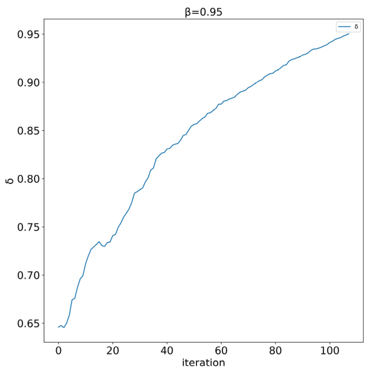
Figure 1. From these outcomes, we have the following observations.
- (1)
As the value of group consensus threshold β increases, the total number of iterations also increase, which reveals that the value of β affects the scores of alternative schemes. At the same time, DMs need to make greater changes. Therefore, it is recommended to adjust the value of β carefully, ensuring that the original decision information remains manageable and does not result in excessive variability.
- (2)
A higher global consensus threshold requires a larger number of iterations, which not only decreases efficiency but also distorts original opinions. For example, when β is set at 0.95, the number of iterations reaches 138. In contrast, when β is set at 0.85, the iterations count decreases to 51, while the degree of group consensus only declines by 0.1. This emphasizes the importance of avoiding high consensus thresholds for group decision-making problems. Instead, the consensus threshold should be determined according to the specific context of the decision-making scenario, guaranteeing that original opinions are primarily preserved.
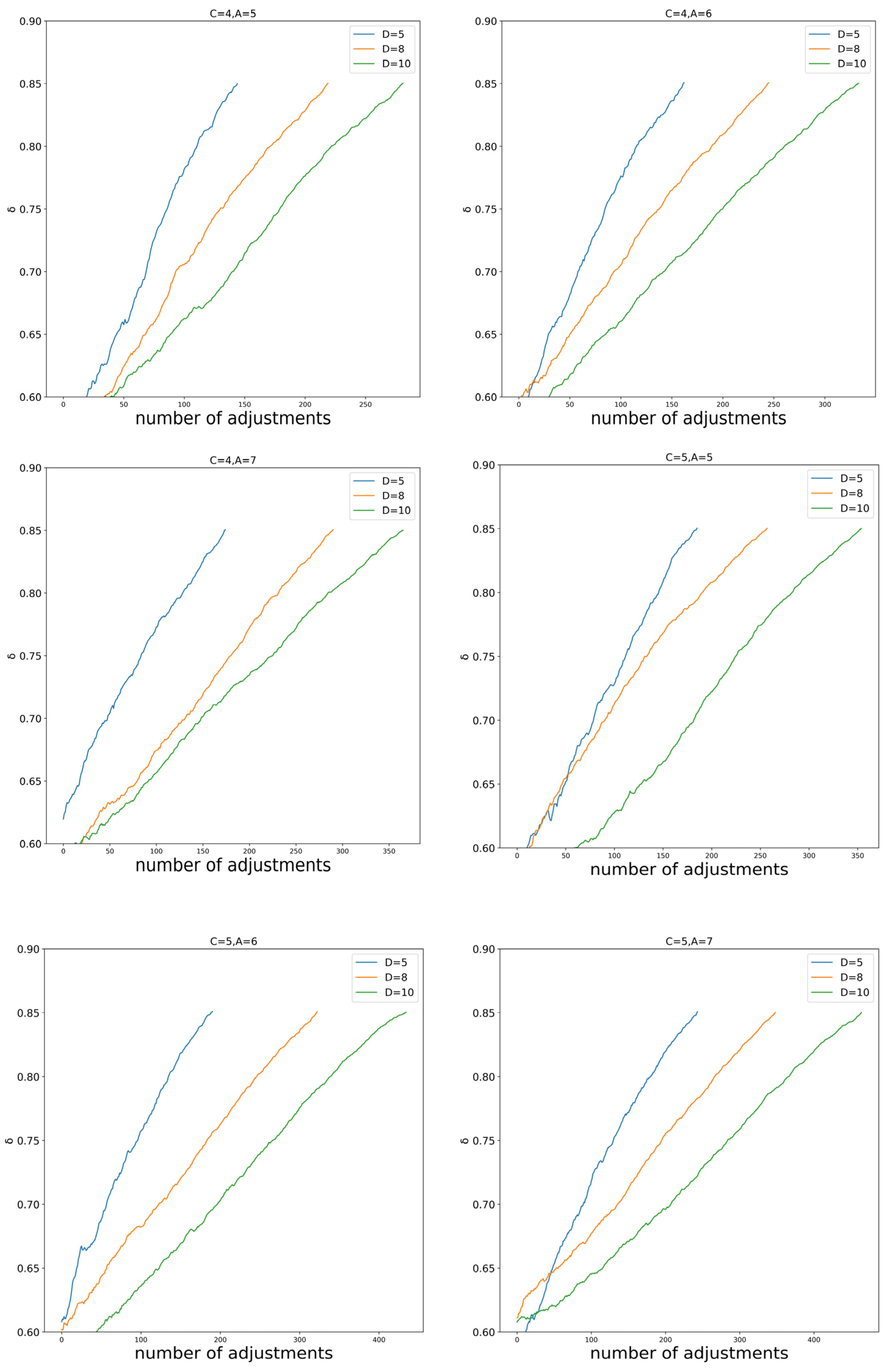
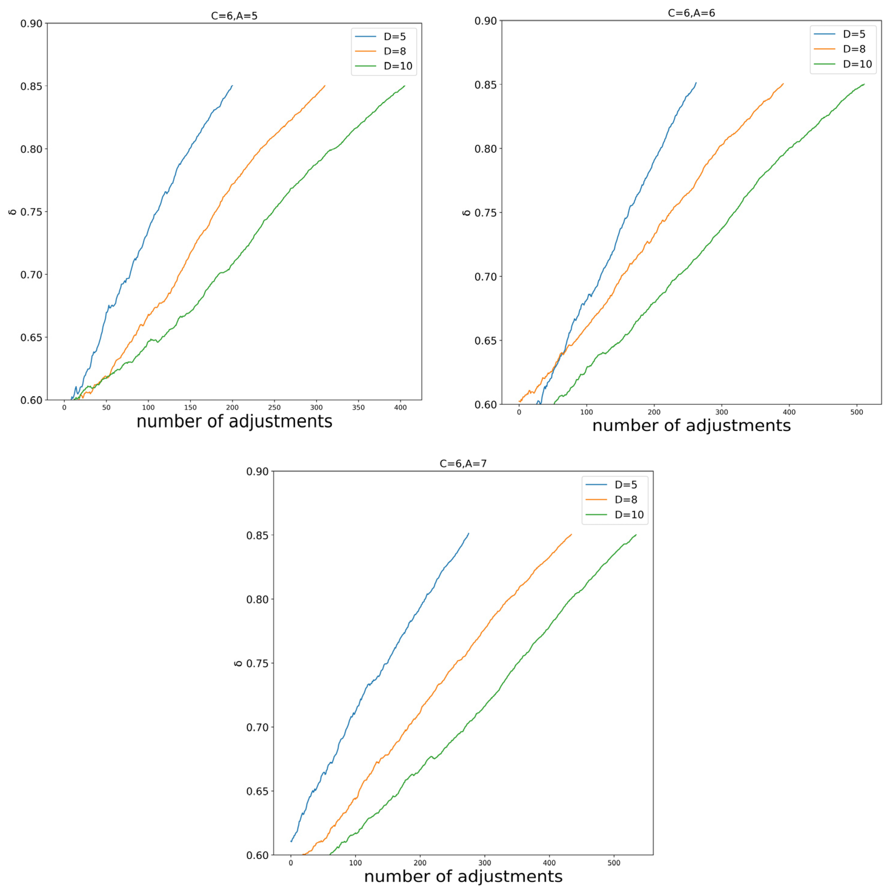
8.1.2. Sensitivity Analysis of DMs, Alternatives, and Attributes
To investigate the proposed model in detail, this section conducts nine simulations with varying input parameters: the number of DMs (D = 5, 8, 10); the number of alternatives (A = 5, 6, 7); and the number of attributes (C = 4, 5, 6). The global consensus threshold
is predefined as 0.85. Initially, we generate the DMs’ evaluation matrix based on HIFLTSs. The values are uniformly and randomly selected from the linguistic terms set
. Subsequently, using different input parameters (D, A, and C), we implement the proposed model and obtain the number of iterations in CRP as well as the global consensus degree, which are depicted in
Figure 2. Based on these outcomes, we have the following observations.
- (1)
With an increase in the number of DMs, there is a significant growth in the number of iterations. For example, when the parameters are set to N = 5, C = 4, and A = 5, the iterations count is 144. Increasing N to 10 causes the iterations to surge to 281. However, the impact of the attribute values and alternative values on the iteration count is not as discernibly pronounced. As a result, it can be observed that the proposed model may have limitations when applied to large-scale group decision-making problems.
- (2)
The group consensus threshold directly influences the total number of iterations. In real decision-making environments, the thresholds are usually fixed beforehand. Therefore, to balance timeliness and a high degree of consensus level, a group could make a simulation and set the appropriate threshold values.
8.2. Discussion
8.2.1. Comparison with [17]
The method we proposed varies from the approach presented in [
17] based on subsequent aspects:
- (1)
The approach in [
17] does not concentrate on the basic operation laws of HITLTSs, and thus it may encounter some limitations when constructing the collective decision matrix. On the one hand, since the method in [
17] cannot deal with scalar multiplication, it gives tacit consent to all decision-makers having the same weight, but it rarely takes place in real-world conditions; on the other hand, only the upper bound and lower bound of each HIFLE are considered when aggregating each decision matrix in [
17], obviously, which may cause the loss of information.
- (2)
The score function and accuracy function in [
17] do not take the hesitancy degree into account, which may lead to counter-intuitive results in some cases.
- (3)
The approach in [
17] overlooks the issues of group consensus. In fact, by applying the method from this paper to the application example in [
17], we determine the global consensus degree
. Such a degree of consensus may not be satisfactory and could potentially result in an unsuccessful final decision.
8.2.2. Comparison with [19]
Ref. [
19] proposed several distance measures for HIFLTSs, and the important distinguishing factors compared with our method are as follows:
- (1)
The method in [
19] also does not consider the basic operation laws of HITLTSs, and thus it may encounter the same limitations as Ref. [
19] when constructing the collective decision matrix.
- (2)
In Ref. [
19], the attribute weights are determined subjectively by DMs, but in our case, we employ the TOPSIS and LP optimization techniques to derive the optimal attribute weights, leading to more precise weightings.
8.2.3. Comparison with Current Score Functions
In this section, we aim to address the application instance discussed in
Section 7 using the current score function and accuracy function. We will demonstrate how the degree of hesitancy impacts the ultimate ranking. The PIS
and NIS
associated with each attribute
can be obtained in
Table 10.
In this segment, our goal is to address the application instance discussed in
Section 7 using the present score function and accuracy function. We will demonstrate how the level of hesitancy impacts the ultimate ranking.
The degree of similarity between the collective decision matrix
R and the PID
H+ and the NID
H− for all alternatives
are listed in
Table 11.
Subsequently, the optimal weights of attributes can be derived as . We can find that there are few differences in the results derived by different score functions and accuracy functions, which verify the importance of considering the degree of hesitancy in score functions and accuracy functions for HITLTSs.
8.2.4. Comparison with Other Ranking Methods
This section aims to demonstrate the credibility of the proposed MULTIMOORA approach compared with the traditional TOPSIS method. The score function considering the degree of hesitancy and correlation measure of HIFLTSs is also utilized to derive the final ranking when using the TOPSIS to solve the application example presented in
Section 7.
The TOPSIS method adopts the vector normalization technique, and the utility value associated with each alternative
can be calculated as:
The final ranking based on the TOPSIS method can be determined by the value of
in
Table 12, which verifies the effectiveness of the proposed MULTIMOORA approach under the HIFLTS environment.
9. Conclusions
Linguistic terms, rather than concrete numerical values, prove to be more effective for DMs when defining intricate and imprecise cognition. HIFLTSs allow DMs to express their uncertainty in a more nuanced and granular manner, capturing not only the degree of membership but also the degree of non-membership and hesitation. This enables a more comprehensive representation of DMs’ preferences and uncertainties, leading to more accurate decision-making processes. However, there are still certain limitations that need to be addressed.
Therefore, this paper proposes a set of new operational laws to address these limitations and enhance the applicability and methodology of HIFLTSs. Additionally, we introduce a novel score function and accuracy function for HIFLTSs that consider the degree of hesitancy, thus rectifying the existing shortcomings. Correlation measures and coefficients are also established to enrich the HIFLTSs’ theoretical framework. We present a MULTIMOORA approach in the HIFLTSs’ environment, which provides more robust, simple, and effective results. To illustrate the functionality of the proposed method, a real-world application example is provided. Furthermore, a detailed comparison with related works and existing approaches demonstrates the advantages and innovation of this study.
The proposed GDM approach based on HIFLTSs has potential applications in various real-world scenarios. For instance, it can assist in the development of teleconsultation decision-making systems for doctors and aid enterprises in selecting suitable suppliers for strategic cooperation. However, there are some limitations in this paper that should be acknowledged:
- (1)
The proposed model appears to be more suitable for small-group decision-making problems based on the simulation results. It is important to explore methods to enhance the efficiency of the proposed models when dealing with large-scale group decision-making problems.
- (2)
The group consensus threshold directly influences the number of iterations in the proposed model. Therefore, addressing the limitation of setting appropriate threshold values is crucial.
- (3)
The CRP does not consider the scenario of DMs’ non-cooperation, which is another limitation that needs to be addressed.
In future studies, we aim to extend the application of the proposed method to areas such as non-cooperation management, feedback mechanism design, and dynamic environment modeling, among others.


