Inverse Graphs in m-Polar Fuzzy Environments and Their Application in Robotics Manufacturing Allocation Problems with New Techniques of Resolvability

Abstract

The inverse in crisp graph theory is a well-known topic. However, the inverse concept for fuzzy graphs has recently been created, and its numerous characteristics are being examined. Each node and edge in m-polar fuzzy graphs (mPFG) include m components, which are interlinked through a minimum relationship. However, if one wants to maximize the relationship between nodes and edges, then the m-polar fuzzy graph concept is inappropriate. Considering everything we wish to obtain here, we present an inverse graph under an m-polar fuzzy environment. An inverse mPFG is one in which each component’s membership value (MV) is greater than or equal to that of each component of the incidence nodes. This is in contrast to an mPFG, where each component’s MV is less than or equal to the MV of each component’s incidence nodes. An inverse mPFG’s characteristics and some of its isomorphic features are introduced. The $\alpha$-cut concept is also studied here. Here, we also define the composition and decomposition of an inverse mPFG uniquely with a proper explanation. The connectivity concept, that is, the strength of connectedness, cut nodes, bridges, etc., is also developed on an inverse mPF environment, and some of the properties of this concept are also discussed in detail. Lastly, a real-life application based on the robotics manufacturing allocation problem is solved with the help of an inverse mPFG.

1. Introduction

1.1. Research Background

The interconnection of a gadobtain can be presented with the help of a graph. Its basis was laid by the well-known Swiss mathematician Euler in 1736 when he mentioned the answer to the seven-bridge problem. There are programs of graph principles for unique regions or networks like electric-powered, PC, road, and picture-capturing networks, etc. A widely known topic in combinatorial optimization and discrete areas is the allocation problem. Some related problems include wiring, printed circuit board issues, load issues, resource task issues, frequency allocation issues, various scheduling issues, and computer register mapping. In technical development, fuzzy graph (FG) theory is important. Many rule-based expert systems for engineers have been created from FG theory. In 1975, Rosenfeld [1] studied relations on fuzzy sets and coined the term fuzzy relations. Graph theory is an essential part of connectivity in some fields of geometry, algebra, topology, number theory, computer science, operations research, and optimization. The only other characteristic of FGs is that their edge MV is less than the minimum of their end node MVs. The literature review below discusses many works based on the allocation problem through graphs and their different variations. However, in real life, there are many problems where vertices and edges cannot be defined in a specific way. Sometimes, they are inverse m-polar fuzzy sets in nature, and their interlinkage can be suitably described by an inverse m-polar fuzzy graph.

1.2. Review of the Literature and Related Works

Zadeh [2] introduced fuzzy sets to deal with ambiguity and fuzziness. Since then, the fuzzy set hypothesis has been investigated in several sequences. Zhang [3,4] introduced bipolar fuzzy sets in 1994. These sets have a wide range of applications in both mathematical and practical situations. Data from numerous sources worldwide have been used to tackle several problems in the real world. This approach for collecting data is a prime example of multipolarity. FGs or bipolar FGs cannot adequately structure this type of polarity. The notion of the m-polar fuzzy set (mPFS) is imposed on graphs to elaborate the various origins in order to simplify the issue. Chen et al. [5] introduced the set concept in an m-dimension fuzzy environment as an extension of bipolar fuzzy sets. Utilizing Zadeh’s procedure, Kauffman [6] fostered a strategy of fuzzy graph theory in 1973. Then, Rosenfeld [1] gave another explanation of a fuzzy graph. Several fuzzy graph concepts have been investigated in [7,8,9,10,11]. An inverse fuzzy graph was first introduced by Borzooei et al. [12]. Then, Poulik and Ghorai [13] studied the concept of an inverse fuzzy mixed graph. Ghorai and Pal introduced for the first time the mPFG, and then they [14,15] introduced m-polar FPGs, dual m-polar FPGs and faces, and m-polar FPGs’ isomorphic features. Then, Mahapatra and Pal introduced the fuzzy coloring of an mPFG [16]. They continued their work on this topic in [17,18]. In Akram et al. [19,20,21], several features of graphs in an m-polar fuzzy environment were examined.

1.3. Motivation of the Work

In real life, many problems have been solved using experimental data that come from different origins or sources. In many situations, it is observed that such data contain multiple attributes for a particular piece of information, i.e., multipolarity. These types of multipolar data cannot be structured well by the conception of intuitionistic or bipolar fuzzy models. For example, consider the allocation problem of some robotic manufacturing on some parameters, such as the following:

(i)

Communication system;

(ii)

Pollution-free zone;

(iii)

Worker availability.

For the nodes and the edges, the parameters may be the following:

(i)

Transportation costs;

(ii)

Availability of labor;

(iii)

The number of workers who service both locations.

In this problem, we consider more than one component for each node and edge, so it is impossible to model this type of situation using a fuzzy set, as there is a single component for this concept. Again, we cannot apply a bipolar or intuitionistic fuzzy graph model, as each edge or node has just two components. Thus, the mPFG models give more flexibility than the fuzzy model or other varieties of fuzzy models. Also, it is very interesting to develop and analyze such types of inverse mPFGs with examples and related theorems.

1.4. Framework of This Study

The structure of this article is as follows: Section 2 contains studies on the preliminary material. In Section 3, we carefully examine a novel idea known as an “inverse 3-polar fuzzy graph”, along with its many features. Section 3.1 properly describes the composition and decomposition of an inverse m-polar fuzzy graph. We introduce a generalized notion of connection on inverse m-polar fuzzy graphs in Section 4 and provide a detailed description of it. In this section, we look at inverse mPF cut nodes and bridges, as well as some of their intriguing features. Then, inverse mPFG is used to address a real-world application based on a production allocation problem in Section 5. Section 6 gives a comparative study of the proposed work. In Section 7, the advantages and limitations of the proposed work are discussed. The work is summarized in Section 8.

1.5. Notations and Symbols

Table 1 gives some notations and abbreviations which are used in the remaining part of the article.

Table 1. Table of Abbreviations.

Full Name	Abbreviated Form
Fuzzy Graph	FG
m-polar Fuzzy Graph	mPFG
Underlying Crisp Graph	UCG
Membership Value	MV
m-polar Fuzzy Set	mPFS
Strength-of-connectedness	SC

2. Preliminaries

Here, we shortly revisit a few definitions related to mPFG, like strong mPFG, complete mPFG, and path in mPFG.

Throughout this article, $p_s:{[0,1]}^m\to [0,1]$ indicates the sth material of projection mapping, and $s=1,2,\dots ,m$ is denoted by $s=1\left(1\right)m$.

Definition 1 ([14]).

Take $G=(\tilde{V},\sigma ,\mu )$ to be an mPFG of the UCG $H^{*}=(\tilde{V},\tilde{E})$, where σ and μ map from $\tilde{V}$ to ${[0,1]}^m$ and $\tilde{V}\times \tilde{V}$ to ${[0,1]}^m$, respectively. Here, σ and μ represent an mPFS of $\tilde{\tilde{V}}$ and $\tilde{V}\times \tilde{V}$, respectively, which maintain the relation $p_s\circ \mu (x,w)\le \{p_s\circ \sigma \left(x\right)\wedge p_s\circ \sigma \left(w\right)\}$ for every $s=1\left(1\right)m$ and $(x,w)\in \tilde{V}\times \tilde{V}$ as well as $\mu (x,w)=$ 0 for every $(x,w)\in (\tilde{V}\times \tilde{V}-\tilde{E})$.

Definition 2 ([15]).

$G=(V,\sigma ,\mu )$ is assigned as a complete mPFG if $p_s\circ \mu (x,w)=\{p_s\circ \sigma \left(x\right)\wedge p_s\circ \sigma \left(w\right)\},$ for every $x,w\in V$ and $s=1\left(1\right)m$.

Definition 3 ([14]).

$G=(V,\sigma ,\mu )$ is assigned as an mPF strong graph if

$$p_s\circ \mu (x,w)=\{p_s\circ \sigma \left(x\right)\wedge p_s\circ \sigma \left(w\right)\},$$

for every $(x,w)\in E$ and $s=1\left(1\right)m$.

Definition 4 ([20]).

Let $G=(V,\sigma ,\mu )$ be an mPFG and $P:x_1,x_2,\dots ,x_k$ be a path in G. $S\left(P\right)$ denotes the strength of P, which is defined as $S\left(P\right)=(\underset{1\le s<j\le k}{min}{p}_1\circ \mu (x_s,x_j)$, $\underset{1\le s<j\le k}{min}{p}_2\circ \mu (x_s,x_j),\dots ,\underset{1\le s<j\le k}{min}{p}_m\circ \mu (x_s,x_j))=({\mu }_1^n(x_s,x_j),{\mu }_2^n(x_s,x_j),\dots ,{\mu }_m^n(x_s,x_j))$.

The strength of the connectedness of a path in-between $x_1$ and $x_k$ is denoted by $CON{N}_G(x_1,x_k)$ and is given as follows:

$$CON{N}_G(x_1,x_k)=(p_1\circ \mu {(x_s,x_j)}^{\infty },p_2\circ \mu {(x_s,x_j)}^{\infty },\dots ,p_m\circ \mu {(x_s,x_j)}^{\infty }),$$

where $(p_i\circ \mu {(x_s,x_j)}^{\infty })=\underset{n\in N}{max}\left({\mu }_i^n(x_s,x_j)\right),i=1,2,\dots ,m$.

Definition 5 ([16]).

For an mPFG, an edge $(x,w),x,w\in V$ is considered independently strong in $G=(V,\sigma ,\mu )$ if $\frac{1}{2}\{p_s\circ \sigma \left(x\right)\wedge p_s\circ \sigma \left(w\right)\}\le p_s\circ \mu (x,w),s=1\left(1\right)m$. If not, it is perceived as weak on its own. The sth component of the strength of an edge $(x,w)$ is defined as

$$p_s\circ I(x,w)=\frac{p_s\circ \mu (x,w)}{p_s\circ \sigma \left(x\right)\wedge p_s\circ \sigma \left(w\right)},s=1\left(1\right)m.$$

Definition 6. 

Take $G=(V,\sigma ,\mu )$ and $G^{\prime }=(V^{\prime },{\sigma }^{\prime },{\mu }^{\prime })$ as two mPFGs of the UCG $G^{*}=(V,E)$ and ${G^{\prime }}^{*}=(V^{\prime },E^{\prime })$, respectively. An isomorphism is a bijection of G and $G^{\prime }$, that is, $g:V\to V^{\prime }$, and satisfies

$$p_s\circ \sigma \left(x\right)=p_s\circ {\sigma }^{\prime }\left(g\left(x\right)\right)and{p}_s\circ \mu (x,w)=p_s\circ {\mu }^{\prime }(g\left(x\right),g\left(w\right))$$

$\forall x,w\in V$ and every $s=1\left(1\right)m$. G is then said to be isomorphic with $G^{\prime }$.

3. Inverse $\mathbf{m}$-Polar Fuzzy Graph

In this section, we discuss a new idea of mPFGs, which have nodes and edges along with an MV such that they fulfill a specific criterion.

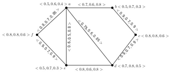
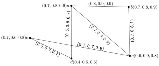
Definition 7. 

Let $G=(V,\sigma ,\mu )$ be an mPFG of the UCG $G^{*}=(\tilde{V},\tilde{E})$, where σ and μ map from $\tilde{V}$ to ${[0,1]}^m$ and $\tilde{V}\times \tilde{V}$ to ${[0,1]}^m$, respectively. Here, σ and μ represent an mPFS of $\tilde{V}$ and $\tilde{V}\times \tilde{V}$, respectively, which maintain the relation $p_s\circ \mu (x,w)\ge \{p_s\circ \sigma \left(x\right)\wedge p_s\circ \sigma \left(w\right)\}$ for every $s=1\left(1\right)m$ and $(x,w)\in \tilde{V}\times \tilde{V}$ as well as $\mu (x,w)=\mathit{0}$ for every $(x,w)\in (\tilde{V}\times \tilde{V}-\tilde{E})$.

Example 1. 

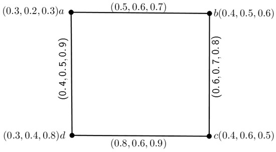
The above definition is depicted through an example, which is given in Figure 1.

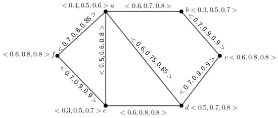
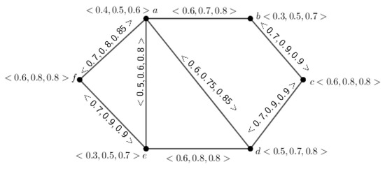
Figure 1. An illustration of inverse 3-polar fuzzy graph.

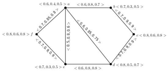
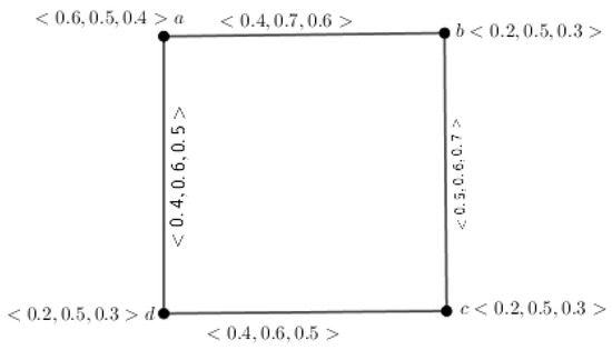
Definition 8. 

Let $G=(V,\sigma ,\mu )$ be an inverse mPFG, having UCG $G^{*}=(V,E)$. Then, G is called a complete inverse mPFG if $E=V\times V$ and $\forall s=1\left(1\right)m$, $p_s\circ \mu (b,d)>\{p_s\circ \sigma \left(b\right)\wedge p_s\circ \sigma \left(d\right)\}$$\forall (b,d)\in V\times V$.

Example 2. 

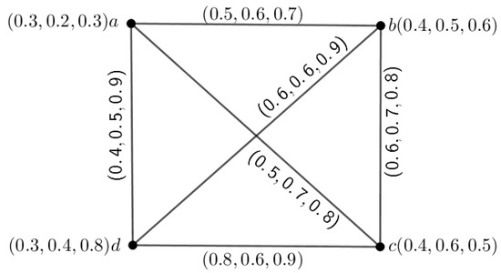
The above definition is illustrated through an example, which is given in Figure 2.

Figure 2. Complete inverse 3-polar fuzzy graph.

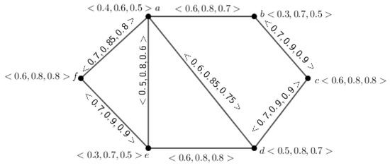
Definition 9. 

Let $G=(V,\sigma ,\mu )$ be an inverse mPFG. Then, the complement of G is indicated by $G^c=(V,{\sigma }^c,{\mu }^c)$, which is conferred by $p_s\circ {\sigma }^c\left(x\right)=p_s\circ \sigma \left(x\right)$ and $p_s\circ {\mu }^c(x,w)=$ $1-p_s\circ \mu (x,w)+(p_s\circ \sigma \left(x\right)\wedge p_s\circ \sigma \left(w\right))$, for $s=1\left(1\right)m$.

Example 3. 

The complement of the inverse 3PFG of Figure 1 is shown in Figure 3.

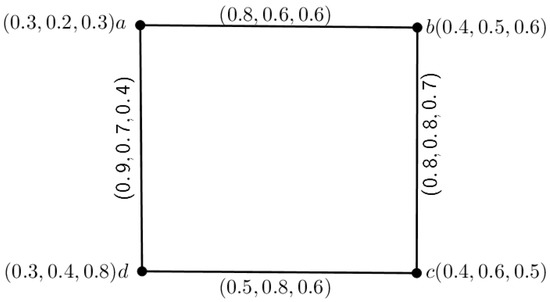
Figure 3. Complement of 3PFG of Figure 1.

Note 1: 

It is clear from the above discussion that the union of inverse mPFG and complement inverse mPFG does not form a complete inverse mPFG.

Definition 10. 

Suppose $G=(V,\sigma ,\mu )$ and $G^{\prime }=(V^{\prime },{\sigma }^{\prime },{\mu }^{\prime })$ are the inverse mPFGs of the UCG $G^{*}=(V,E)$ and ${G^{\prime }}^{*}=(V^{\prime },E^{\prime })$, respectively. An isomorphism is a bijection between G and $G^{\prime }$, that is, $g:V\to V^{\prime }$, and satisfies

$$p_s\circ \sigma \left(x\right)=p_s\circ {\sigma }^{\prime }\left(g\left(x\right)\right)\mathrm{and}{p}_s\circ \mu (x,w)=p_s\circ {\mu }^{\prime }(g\left(x\right),g\left(w\right))$$

$\forall x,w\in V$ and for every $s=1\left(1\right)m$. Then, G is said to be isomorphic to $G^{\prime }$.

Definition 11. 

Let $G=(V,\sigma ,\mu )$ and $G^{\prime }=(V^{\prime },{\sigma }^{\prime },{\mu }^{\prime })$ be two inverse mPFGs. Then, $G^{\prime }$ is called a partial inverse mPFG of G if $V^{\prime }\subseteq V$ and $p_s\circ {\sigma }^{\prime }\left(x\right)\le p_s\circ \sigma \left(x\right)$, for all $a\in V^{\prime }$ as well as $p_s\circ {\mu }^{\prime }(x,w)\le p_s\circ \mu (x,w)$, for all $(x,w)\in E^{\prime }$.

Definition 12. 

Let $G=(\tilde{V},\sigma ,\mu )$ and $G^{\prime }=(V^{\prime },{\sigma }^{\prime },{\mu }^{\prime })$ be two inverse mPFGs. Then, $G^{\prime }$ is called an inverse mPF subgraph of G if $V^{\prime }\subseteq V$ and $p_s\circ {\sigma }^{\prime }\left(x\right)=p_s\circ \sigma \left(x\right)$, for all $x\in V^{\prime }$ as well as $p_s\circ {\mu }^{\prime }(x,w)=p_s\circ \mu (x,w)$, for all $(x,w)\in E^{\prime }$.

Definition 13. 

Let $G=(V,\sigma ,\mu )$ be an inverse mPFG. Let $a\in V$. Then, the order of x is indicated by $d\left(a\right)$ and conferred by $p_s\circ d\left(x\right)={\sum }_{(x,w)\in E}{p}_s\circ \mu (x,w)$, for $s=1\left(1\right)m$. The total degree of the vertex x is indicated by $d_T\left(x\right)$ and is conferred by $p_s\circ d_T\left(x\right)=p_s\circ d\left(x\right)+p_s\circ \sigma \left(x\right),$ for $s=1\left(1\right)m$. The degree of G is indicated by $d\left(G\right)$ and is conferred by $p_s\circ d\left(G\right)={\sum }_{\left(x\right)\in V}{p}_s\circ \sigma \left(x\right)$, for $s=1\left(1\right)m$. The size of G is indicated by $S\left(G\right)$ and conferred by $p_s\circ S\left(G\right)={\sum }_{(x,w)\in E}{p}_s\circ \mu (x,w)$, for $s=1\left(1\right)m$.

Definition 14. 

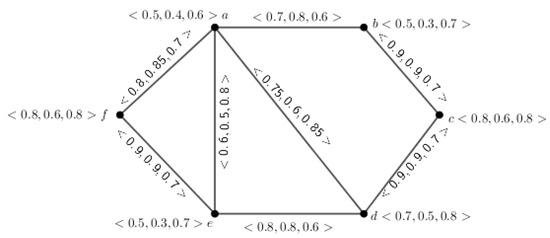
Let $G=(V,\sigma ,\mu )$ be an inverse mPFG. Then, α-cut, $\alpha \in [0,1]$, is indicated as $G_{\alpha }$ and is defined by ${\sigma }_{\alpha }=\{a\in V:p_s\circ \sigma \left(a\right)\ge \alpha ,i=1,2,\dots ,m\}$ and ${\mu }_{\alpha }=\{(x,w)\in E:p_s\circ \sigma (x,w)\ge \alpha ,i=1,2,\dots ,m\}$.

In ordinary mPFG theory, we know that every $\alpha$-cut, $\alpha \in [0,1]$, is a crisp graph. But, in our proposed model, this is not generally true; it is possible that not every $\alpha$-cut, $\alpha \in [0,1]$, of an inverse mPFG is a crisp graph. This is illustrated through Example 4.

Example 4. 

Let us consider $\alpha =(0.25,0.25,0.25)$. Then, the α-cut of the mPFG of Figure 1 is shown in Figure 4.

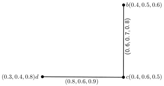
Figure 4. The $0.25$-cut 3PFG of Figure 1.

Theorem 1. 

Let $G=(V,\sigma ,\mu )$ be an inverse mPFG of an UCG and $\alpha \in [0,1]$. If for any $a\in V$, $p_s\circ \sigma \left(a\right)\ge \alpha$ and $p_s\circ \mu (x,w)\ge \alpha$, for every $(x,w)\in E$ and for each $s=1\left(1\right)m$, then $G_{\alpha }$ is a crisp graph.

Proof. 

Suppose $p_s\circ \mu (x,w)\ge \alpha$ for each $=1\left(1\right)m$. Then, we must have $p_s\circ \sigma \left(x\right)\ge \alpha$ and $p_s\circ \sigma \left(w\right)\le \alpha$, for each $=1\left(1\right)m$, or $p_s\circ \sigma \left(x\right)\le \alpha$ and $p_s\circ \sigma \left(w\right)\ge \alpha$, for each $=1\left(1\right)m$. It is clear for case 1.

For the second case, if $p_s\circ \sigma \left(x\right)\le \alpha$ and $p_s\circ \sigma \left(w\right)\ge \alpha$, for $s=1\left(1\right)m$, then we obtain $p_s\circ \mu (x,w)\le \alpha$, for $s=1\left(1\right)m$, which is a contradiction.

Hence, $G_{\alpha }$ is a crisp graph.    □

Theorem 2. 

Let $G=(V,\sigma ,\mu )$ be an inverse mPFG of an UCG. If there exists a $\beta \in [0,1]$ and an edge $(x,w)$ such that $p_s\circ \mu (x,w)\ge p_s\circ \sigma \left(x\right)\wedge p_s\circ \sigma \left(w\right)$, for $s=1\left(1\right)m$, then $G_{\beta }$ is not a crisp graph.

Proof. 

If possible, let $\forall \alpha \in [0,1]$$G_{\alpha }$ be a crisp graph. Then, we must have $G_{\alpha }$ as an mPFG. Then, from the definition of mPFG, we have $\forall s=1\left(1\right)m$, $p_s\circ \mu (x,w)\le \{p_s\circ \sigma \left(x\right)\wedge p_s\circ \sigma \left(w\right)\}$$\forall (x,w)\in \widetilde{V\times V}$. Again, from the definition of an inverse mPFG, we obtain $\forall s=1\left(1\right)m$, $p_s\circ \mu (x,w)\ge \{p_s\circ \sigma \left(x\right)\wedge p_s\circ \sigma \left(w\right)\}$$\forall (x,w)\in \widetilde{V\times V}$.

Combining both of them, we obtain, $\forall s=1\left(1\right)m$, $p_s\circ \mu (x,w)=\{p_s\circ \sigma \left(x\right)\wedge p_s\circ \sigma \left(w\right)\}$$\forall (x,w)\in \widetilde{V\times V}$, which is a contradiction, hence the theorem.    □

3.1. Decomposition and Composition of Inverse m-Polar Fuzzy Graph

3.1.1. Decomposition

By collecting each component from the inverse m-polar fuzzy graph, we can construct the m number of fuzzy graphs. An inverse m-polar fuzzy graph, G, is used for this purpose. The inverse m-polar fuzzy graph G can be created by building the graph $G_i$ and edges using the ith component of the membership values of the nodes in the fuzzy graph $G_1,G_2,\dots ,G_m$. The following example is used to demonstrate this concept.

Example 5. 

The above definition is depicted through an example, which is given in Figure 5.

Figure 5. An Inverse 3-polar fuzzy graph illustrates the decomposition.

Here, we consider the inverse 3PFG shown in Figure 6. Taking the first component for each node and edge of G, we obtain an inverse fuzzy graph $G_1$. Taking the second component for each node and edge of G, we obtain an inverse fuzzy graph $G_2$. Finally, taking the third component for each node and edge of G, we obtain an inverse fuzzy graph $G_3$. Hence, we obtain three inverse fuzzy graphs from G. All those inverse fuzzy graphs are shown in Figure 6.

Figure 6. Inverse fuzzy graphs $G_1,G_2,G_3$ obtained by decomposition of 3PFG of Figure 5.

3.1.2. Composition

Think about the $G_1,G_2,\dots ,G_m$, where m is the number of inverse fuzzy graphs. Their corresponding underlying crisp graphs $G_1^{*},G_2^{*},\dots ,G_m^{*}$ are isomorphic. We can suppose that there are m spaces for m objects to be filled because we have m fuzzy graphs. The $m!$ technique can be used for this purpose. Thus, for $m!$ integers, we can obtain inverse mPFGs. The following example illustrates this idea.

Example 6. 

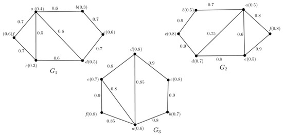
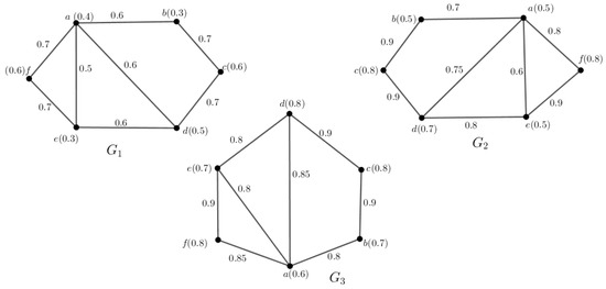
To illustrate the above discussion, we consider three inverse fuzzy graphs $G_1,G_2,G_3$, the crisp graphs of which are isomorphic, as shown in Figure 7.

Figure 7. Inverse fuzzy graphs $G_1,G_2,G_3$ whose crisp graphs are isomorphic.

To convert the graph into an inverse 3PFG, we can imagine that there are three places that would be filled by three objects. This can be achieved in the following way:

$$H_1=G_1{G}_2{G}_3$$

$$H_2=G_2{G}_3{G}_1$$

$$H_3=G_3{G}_1{G}_2$$

$$H_4=G_1{G}_3{G}_2$$

$$H_5=G_2{G}_1{G}_3$$

$$H_6=G_3{G}_2{G}_1$$

Hence, we obtain six inverse 3PFGs, which are shown in Figure 8, Figure 9, Figure 10, Figure 11, Figure 12 and Figure 13.

Figure 8. Inverse 3-polar fuzzy graph $H_1$.

Figure 9. Inverse 3-polar fuzzy graph $H_2$.

Figure 10. Inverse 3-polar fuzzy graph $H_3$.

Figure 11. Inverse 3-polar fuzzy graph $H_4$.

Figure 12. Inverse 3-polar fuzzy graph $H_5$.

Figure 13. Inverse 3-polar fuzzy graph $H_6$.

4. Connectivity in Inverse $\mathit{m}$-Polar Fuzzy Graphs

Definition 15. 

Let $G=(V,\sigma ,\mu )$ be an inverse mPFG. Then, a path P is an alternating sequence of distinct nodes $u_0,u_1,u_2,\dots ,u_n$ such that $p_s\circ \mu (u_j,u_{j+1})>0$, for $s=1\left(1\right)m$ and $j=0\left(1\right)n$. The strength of a path is the minimum of the MV of each component that is $p_s\circ S\left(P_{(x,w)}\right)=\underset{d\in P}{min}{p}_s\circ \sigma \left(d\right)$, for $s=1\left(1\right)m$, for the path x to w. The strength of connectedness (SC) between two nodes, for example, $x,w$, is given as $p_s\circ {\sigma }_G^{\infty }(x,w)=\underset{P_{(x,w)}}{sup}{p}_s\circ S\left(P_{(x,w)}\right)$, for $s=1\left(1\right)m$.

Note 2: 

A path between x and w is denoted as $P_{(x,w)}$.

Note 3: 

As $p_s\circ S\left(P_{(x,w)}\right)=\underset{d\in P}{min}{p}_s\circ \sigma \left(d\right)$, for $s=1\left(1\right)m$, we have $p_s\circ {\sigma }_G^{\infty }(x,w)\le p_s\circ \sigma \left(x\right)\wedge p_s\circ \sigma \left(w\right)$, for $s=1\left(1\right)m$.

Theorem 3. 

Let $G=(V,\sigma ,\mu )$ be an inverse mPFG. If any two nodes $x,w$ are connected through an edge, then $p_s\circ {\sigma }_G^{\infty }(x,w)=p_s\circ \sigma \left(x\right)\wedge p_s\circ \sigma \left(w\right)$, for $s=1\left(1\right)m$.

Proof. 

To prove this theorem, we consider two cases.

Case 1: 

Let $P_{(x,w)}$ be the only path between x and w. Then, we can easily obtain that $p_s\circ {\sigma }_G^{\infty }(x,w)=p_s\circ S\left(P\right)=p_s\circ \sigma \left(x\right)\wedge p_s\circ \sigma \left(w\right)$, for $s=1\left(1\right)m$.

Case 2: 

Let there exist more than one path between x and w. Let $P_{(x,w)}^{\prime }$ be another path between x and w. Suppose $d\in P_{(x,w)}^{\prime }$.

Case 2.1: 

Let $p_s\circ \sigma \left(d\right)<p_s\circ \sigma \left(x\right)\wedge p_s\circ \sigma \left(w\right)$, for $s=1\left(1\right)m$. Then, $p_s\circ S\left(P^{\prime }\right)\le p_s\circ \sigma \left(d\right)<p_s\circ \sigma \left(x\right)\wedge p_s\circ \sigma \left(w\right)$, for $s=1\left(1\right)m$. Hence, $p_s\circ {\sigma }_G^{\infty }(x,w)=p_s\circ \sigma \left(x\right)\wedge p_s\circ \sigma \left(w\right)$, for $s=1\left(1\right)m$.

Case 2.2: 

Let $p_s\circ \sigma \left(d\right)\ge p_s\circ \sigma \left(x\right)\wedge p_s\circ \sigma \left(w\right)$, for $s=1\left(1\right)m$. Therefore, $p_s\circ S\left(P^{\prime }\right)=p_s\circ \sigma \left(x\right)\wedge p_s\circ \sigma \left(w\right)$, for $s=1\left(1\right)m$. Hence, $p_s\circ {\sigma }_G^{\infty }(x,w)=p_s\circ \sigma \left(x\right)\wedge p_s\circ \sigma \left(w\right)$, for $s=1\left(1\right)m$.

Combining all these together, we can say that if any two nodes $x,w$ are connected through an edge, then $p_s\circ {\sigma }_G^{\infty }(x,w)=p_s\circ \sigma \left(x\right)\wedge p_s\circ \sigma \left(w\right)$, for $s=1\left(1\right)m$.    □

Definition 16. 

Let $G=(V,\sigma ,\mu )$ be a connected inverse mPFG and $c\in V$ be any node. Then, c is called an inverse fuzzy cut node if there exist two distinct nodes $d,e$ such that for $s=1\left(1\right)m$,

$$p_s\circ {\sigma }_{G^{\prime }}^{\infty }(d,e)<p_s\circ {\sigma }_G^{\infty }(d,e),$$

where $G^{\prime }=G-\left\{c\right\}$. If G does not consist of any inverse mPF cut nodes, then it is said to be made of inverse mPF blocks.

Example 7. 

The above definition is depicted through an example in which we consider an inverse 3PFG shown in Figure 14.

Figure 14. Inverse 3-polar fuzzy graph G to describe Definition 16.

Here, if we want to calculate the strength of connectedness between a and e, then we see that there are three paths from a to e. They are namely $a-b-c-e$, $a-d-e$, $a-c-e$. Now, the SC between a and e is $(0.6,0.6,0.8)$. If we delete the node c that supposes $G^{\prime }=G-\left\{c\right\}$, then the SC between a and e in $G^{\prime }$ is $(0.4,0.5,0.6)$. Therefore, SC is decreased in $G^{\prime }$. Hence, c is an inverse 3PF cut node.

Theorem 4. 

Let $G=(V,\sigma ,\mu )$ be a complete inverse mPFG. Then, G is an inverse mPF block.

Proof. 

From Theorem 3, we have that if any two nodes $x,w$ are connected through an edge, then $p_s\circ {\sigma }_G^{\infty }(x,w)=p_s\circ \sigma \left(x\right)\wedge p_s\circ \sigma \left(w\right)$, for $s=1\left(1\right)m$. Therefore, the removal of any nodes d other than $x,w$ does not change the connectedness between $x,w$. Hence, d is not an inverse mPF cut node.

Again, in a complete inverse mPFG, $E=V\times V$, every two nodes are connected by an edge. So, no nodes are inverse mPF cut nodes of G. Therefore, G is an inverse mPF block.

The opposite of the aforementioned theorem might not be true, as shown by an example.    □

Example 8. 

The above theorem is depicted by an example for which we consider an inverse 3PFG shown in Figure 15.

Figure 15. Inverse 3-polar fuzzy graph G to describe Example 8.

Here, we see that for the SC between any two nodes $x,w\in V$, we have $p_s\circ {\sigma }_G^{\infty }(x,w)=p_s\circ \sigma \left(x\right)\wedge p_s\circ \sigma \left(w\right)$, for $s=1\left(1\right)m$. So, the SC does not decrease if we remove any nodes in V. Hence, G has no 3PF cut nodes. Therefore, it is a 3PF block. Again, clearly, it is not an inverse complete 3PFG.

Definition 17. 

Let $G=(V,\sigma ,\mu )$ be a connected inverse mPFG. Then, $(u,v)$ is called an inverse mPF bridge if there exists two distinct nodes $d,e$ such that for $s=1\left(1\right)m$,

$$p_s\circ {\sigma }_{G^{\prime }}^{\infty }(d,e)<p_s\circ {\sigma }_G^{\infty }(d,e),$$

where $G^{\prime }=G-\left\{(u,v)\right\}$.

Example 9. 

The above definition is depicted through an example for which we consider an inverse 3PFG, shown in Figure 14.

We want to calculate the SC between a and e. We assume that there are three paths from a to e. These are $a-b-c-e$, $a-d-e$, and $a-c-e$. Now, the SC between a and e is $(0.6,0.6,0.8)$. If we delete the edge $(c,e)$, that is, if we suppose $G^{\prime }=G-\left\{(c,e)\right\}$, then the SC between a and e in $G^{\prime }$ is $(0.4,0.5,0.6)$. This shows that SC is decreased in $G^{\prime }$. Hence, $(c,e)$ is an inverse 3PF bridge.

Theorem 5. 

Let $G=(V,\sigma ,\mu )$ be a connected inverse mPFG and $(x,w)\in E$. Then, $(x,w)$ is an inverse mPF bridge iff either $(x,w)$ is a crisp bridge or for every path P between b and c of $G^{\prime }=G-\left\{(x,w)\right\}$ there exists $d\in P$ such that $p_s\circ \sigma \left(d\right)<p_s\circ \sigma \left(x\right)\wedge p_s\circ \sigma \left(w\right)$, for $s=1\left(1\right)m$.

Proof. 

Let $(x,w)$ be an inverse mPF bridge and $G^{\prime }=G-\left\{(x,w)\right\}$. Since $(x,w)$ is an inverse mPF bridge, there thus exist two distinct nodes $d,e$ such that for $s=1\left(1\right)m$,

$$p_s\circ {\sigma }_{G^{\prime }}^{\infty }(d,e)<p_s\circ {\sigma }_G^{\infty }(d,e).$$

If $p_s\circ {\sigma }_{G^{\prime }}^{\infty }(d,e)=0$, for $s=1\left(1\right)m$, then d and e are not connected by any path in $G^{\prime }$. Therefore, $(x,w)$ is a crisp bridge.

If $p_s\circ {\sigma }_{G^{\prime }}^{\infty }(d,e)>0$ and $p_s\circ {\sigma }_{G^{\prime }}^{\infty }(d,e)<p_s\circ {\sigma }_G^{\infty }(d,e)$, for $s=1\left(1\right)m$, then $(x,w)$ are connected by at least one path in $G^{\prime }$. If possible, let u be such that $p_s\circ \sigma \left(u\right)\ge p_s\circ \sigma \left(x\right)\wedge p_s\circ \sigma \left(w\right)$, for $s=1\left(1\right)m$. Then, $p_s\circ S\left(P^{\prime }\right)\ge p_s\circ \sigma \left(x\right)\wedge p_s\circ \sigma \left(w\right)$, for $s=1\left(1\right)m$. So, $p_s\circ {\sigma }_{G^{\prime }}^{\infty }(d,e)\ge p_s\circ \sigma \left(x\right)\wedge p_s\circ \sigma \left(w\right)$, for $s=1\left(1\right)m$. Since $(x,w)$ is an inverse mPF bridge, therefore, it is an edge of every strong path from x to w. Hence, $p_s\circ {\sigma }_{G^{\prime }}^{\infty }(d,e)\le p_s\circ \sigma \left(x\right)\wedge p_s\circ \sigma \left(w\right)$, for $s=1\left(1\right)m$. So, $p_s\circ {\sigma }_{G^{\prime }}^{\infty }(d,e)\ge p_s\circ {\sigma }_G^{\infty }(d,e)$, for $s=1\left(1\right)m$, which is a contradiction. Hence, for every path P in between x and w of $G^{\prime }=G-\left\{(x,w)\right\}$, there exists $d\in P$ such that $p_s\circ \sigma \left(d\right)<p_s\circ \sigma \left(x\right)\wedge p_s\circ \sigma \left(w\right)$, for $s=1\left(1\right)m$.    □

Theorem 6. 

Let $G=(V,\sigma ,\mu )$ be an inverse mPFG having UCG $G^{*}=(V,E)$ and $(x,w)\in E$. Then, $(x,w)$ is an inverse mPF bridge in G iff $p_s\circ {\sigma }_{G^{\prime }}^{\infty }(x,w)<p_s\circ {\sigma }_G^{\infty }(x,w)$, for $s=1\left(1\right)m$, where $G^{\prime }=G-\left\{(x,w)\right\}$.

Proof. 

Let $(x,w)$ be an inverse mPF bridge. Then, from Theorem 5, we find that either $(x,w)$ is crisp bridge or in every path P between x and w in $G^{\prime }$ there exists a node d such that $p_s\circ \sigma \left(d\right)<p_s\circ \sigma \left(x\right)\wedge p_s\circ \sigma \left(w\right)$, for $s=1\left(1\right)m$. Hence, $p_s\circ S\left(P\right)\le p_s\circ \sigma \left(d\right)<p_s\circ \sigma \left(x\right)\wedge p_s\circ \sigma \left(w\right)=p_s\circ {\sigma }_G^{\infty }(x,w)$, for $s=1\left(1\right)m$. Therefore, $p_s\circ {\sigma }_{G^{\prime }}^{\infty }(x,w)<p_s\circ {\sigma }_G^{\infty }(x,w)$, for $s=1\left(1\right)m$, where $G^{\prime }=G-\left\{(x,w)\right\}$.

Conversely, $p_s\circ {\sigma }_{G^{\prime }}^{\infty }(x,w)<p_s\circ {\sigma }_G^{\infty }(x,w)$, for $s=1\left(1\right)m$, where $G^{\prime }=G-\left\{(x,w)\right\}$. Then, it is easy to verify that $(x,w)$ is an inverse mPF bridge in G.    □

5. Application

In many real linked graphical systems where the vertices and edges are both part of an inverse m-polar fuzzy information, the inverse mPFG is a crucial mathematical structure that represents the information. In this section, we attempt to resolve a specific type of allocation problem utilizing a cut node in inverse mPFG.

5.1. Model Construction

Robotics is an important issue for every human body nowadays. The engineering field of robotics deals with the creation, design, production, and use of robots. The goal of the area of robotics is to develop smart machines that can help people in a number of ways. There are many different types of robotics. They boost productivity because robots are programmed to carry out repetitive activities endlessly, but the human brain is not. Robots are used in industries to carry out boring, redundant jobs, freeing up workers to take on more difficult duties and even pick up new abilities.

Here, five towns $a_1,a_2,\dots ,a_5$ are regarded as nodes. If there is a common worker between two nodes, there will be an edge between them. The allocation problem is solved using an inverse 3PFG $G=(V,\sigma ,\mu )$. In this model, the first component is the communication system, the second is the pollution-free zone, and the third is the worker’s availability. This is an inverse 3PFG model. Here, every advantage is based on the factors of transportation costs, labor resources, and workers who service both locations. Therefore, the MVs of each node’s components are listed in Table 2.

Table 2. Vertex membership values of G.

Node	Membership Values
$a_1$	$(0.4,0.5,0.3)$
$a_2$	$(0.5,0.4,0.2)$
$a_3$	$(0.3,0.2,0.1)$
$a_4$	$(0.4,0.5,0.3)$
$a_5$	$(0.7,0.5,0.2)$
$a_6$	$(0.3,0.5,0.1)$
$a_7$	$(0.6,0.5,0.4)$
$a_8$	$(0.7,0.6,0.2)$

An mPFG is symmetric if and only if $\mu (a,b)=\mu (b,a)$, where $\mu (a,b)$ denotes the MV of the edge $(a,b)$. The 3PFS is $E=\{(a_1,a_2),(a_1,a_6),(a_1,a_8),(a_2,a_3),(a_3,a_4),(a_4,a_5),(a_4,a_7),(a_5,a_7),(a_5,a_6)\}$. The MVs of the edges are taken into account based on factors such as transportation costs, the availability of labour, and the number of workers who are working in both locations. The MVs of edges are taken into consideration in Table 3, for instance.

Table 3. Edge membership values of G.

Edge	Membership Values
$(a_1,a_2)$	$(0.3,0.4,0.2)$
$(a_1,a_6)$	$(0.3,0.3,0.1)$
$(a_1,a_8)$	$(0.3,0.3,0.2)$
$(a_2,a_3)$	$(0.2,0.2,0.1)$
$(a_2,a_8)$	$(0.5,0.4,0.2)$
$(a_3,a_4)$	$(0.3,0.2,0.1)$
$(a_3,a_7)$	$(0.3,0.1,0.1)$
$(a_4,a_5)$	$(0.4,0.5,0.1)$
$(a_4,a_7)$	$(0.4,0.4,0.2)$
$(a_5,a_6)$	$(0.2,0.2,0.1)$
$(a_5,a_7)$	$(0.6,0.4,0.2)$
$(a_6,a_7)$	$(0.3,0.4,0.1)$
$(a_7,a_8)$	$(0.5,0.4,0.2)$

The model inverse 3PFG is given in Figure 16.

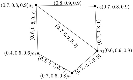
Figure 16. Model inverse 3-polar fuzzy graph G.

Here, an algorithm is given in Algorithm 1 to find the best suitable location for robotics manufacturing allocation.    

Algorithm 1: An algorithm to find the best suitable location for robotic manufacturing allocation.

Input: An inverse mPFG $G=(V,\sigma ,\mu )$. Output: Find the best suitable location for robotic manufacturing allocation. Step 1: Put the membership value of vertices $a_j$, $j=1,2,\dots ,n$. Step 2: Put the membership value of edges which satisfied $p_i\circ \mu (a_j,a_k)\ge inf\{p_i\circ \sigma \left(a_j\right),p_i\circ \sigma \left(a_k\right)\}$, $i=1,2,\dots ,m$. Step 3: Find the path between any two nodes of G. Step 4: Find the SC between any path of G. Step 5: Find the cut-vertex of G.

5.2. Illustration of Membership Values

The paths between the vertices $a_1$ and $a_5$ in G are $P_{(a_1,a_5)}^1:a_1-a_2-a_3-a_5$, $P_{(a_1,a_5)}^2:a_1-a_3-a_5$, and $P_{(a_1,a_5)}^3:a_1-a_4-a_5$, and their respective strengths using the formula $p_s\circ S\left(P_{(u,v)}^j\right)=mi{n}_{w\in P}\{p_s\circ \sigma \left(w\right)\}$, for $i=1\left(1\right)3$ (where j indicates the path number), are $S\left(P_{(a_1,a_5)}^1\right)=(0.6,0.6,0.8)$, $S\left(P_{(a_1,a_5)}^2\right)=(0.6,0.6,0.8)$, and $S\left(P_{(a_1,a_5)}^3\right)=(0.4,0.5,0.6)$. Therefore, the SC between the vertices $a_1$ and $a_5$ is ${\sigma }_G^{\infty }(a_1,a_5)=(0.6,0.6,0.8)$.

Similarly, the paths between the vertices $a_1$ and $a_4$ in G are $P_{(a_1,a_4)}^1:a_1-a_2-a_3-a_5-a_4$, $P_{(a_1,a_4)}^2:a_1-a_3-a_5-a_4$, and $P_{(a_1,a_4)}^3:a_1-a_4$, and their respective strengths are $S\left(P_{(a_1,a_4)}^1\right)=(0.4,0.5,0.6)$, $S\left(P_{(a_1,a_4)}^2\right)=(0.4,0.5,0.6)$, and $S\left(P_{(a_1,a_4)}^3\right)=(0.4,0.5,0.6)$. Therefore, the SC between the vertices $a_1$ and $a_4$ is ${\sigma }_G^{\infty }(a_1,a_4)=(0.4,0.5,0.6)$. So, the SCs of all pairs of vertices are given in Table 4.

Table 4. SC of each pair of vertices of G.

Pair of Vertices	SC
$(a_1,a_5)$	$(0.6,0.6,0.8)$
$(a_1,a_4)$	$(0.4,0.5,0.6)$
$(a_1,a_3)$	$(0.6,0.8,0.8)$
$(a_1,a_2)$	$(0.7,0.8,0.9)$
$(a_2,a_5)$	$(0.6,0.6,0.8)$
$(a_2,a_4)$	$(0.4,0.5,0.6)$
$(a_2,a_3)$	$(0.6,0.8,0.8)$
$(a_3,a_5)$	$(0.6,0.6,0.8)$
$(a_3,a_4)$	$(0.4,0.5,0.6)$
$(a_4,a_5)$	$(0.4,0.5,0.6)$

Now, if we delete the vertex $a_3$ in G, then we have a different figure, say $G^{\prime }=G-\left\{a_3\right\}$, which is shown in Figure 2. Thereafter, we determined the SC in between each pair of vertices in $G^{\prime }$ in the following way:

The path between the vertices $a_1$ and $a_5$ in $G^{\prime }$ is $a_1-a_4-a_5$, with an SC ${\sigma }_{G^{\prime }}^{\infty }(a_1,a_5)=(0.4,0.5,0.6)$. Similarly, the SCs of the other pairs in $G^{\prime }$ are ${\sigma }_{G^{\prime }}^{\infty }(a_2,a_5)=(0.4,0.5,0.6)$ and ${\sigma }_{G^{\prime }}^{\infty }(a_4,a_5)=(0.4,0.5,0.6)$. Clearly, we can see that the SC in G is decreased in $G^{\prime }$. Hence, $a_3$ is an inverse 3PF cut node.

5.3. Decision Making

We may conclude that town $a_3$ is the best-suited location to develop a robotics manufacturing facility among all the towns taken into consideration in our suggested model, since it is the only cut node in the model’s inverse 3PFG G. Through the description above, we may infer that the cut node in the inverse mPFG truly matters in this kind of allocation problem. In addition, we acknowledge that cut nodes in inverse mPFGs are more suitable for allocation problems than cut nodes in inverse FGs.

6. Comparative Study

At first, Borzooei et al. [12] introduced an inverse graph for fuzzy graph theory. In their model, they only considered a single component for each node as well as edges. Next, Poulik and Ghorai [13] studied inverse graphs for the mixed fuzzy graph. They considered directed as well as undirected edges in a fuzzy graph. They considered only a single component as a membership value of a vertex and edge. All of them studied inverse graphs for fuzzy graph theory. So, none of the results discussed earlier are applicable when the model is considered in another environment, like in inverse m-polar fuzzy sets. This is why the proposed model in this paper plays a significant role in obtaining better results in such situations.

7. Advantages and Limitations of the Proposed Work

The following are some of the advantages of the proposed work:

(i)

Anyone can analyze the membership values in a multi-polar inverse fuzzy environment in a certain way.

(ii)

Many important definitions and theorems are presented in this study that are very useful.

(iii)

A real application of an inverse m-polar fuzzy model using the concept of SC is described, through which we solve an allocation problem called robotic manufacturing allocation.

Some of the limitations of this study are given as follows:

(i)

This work mainly focuses on the SC concept in inverse m-polar fuzzy environments.

(ii)

If the membership values are available as the interval-valued m-polar fuzzy environments, then the proposed method is not applicable.

(iii)

Negative membership values are also not investigated in the proposed study.

8. Conclusions

The inverse mPFG and some of its fascinating facts have been introduced in this article. A few inverse mPFG complements and isomorphic qualities have been introduced. Here, the idea of the alpha-cut has also been researched. Here, we also provide a highly specialized definition for the composition and decomposition of an inverse mPFG. The idea of connectivity, which includes connection strength, cut nodes, bridges, etc., is likewise established in an inverted mPFG context. Finally, using inverse mPFG, a real-world application based on a production allocation problem is resolved. We shall extend our investigation on inverse graphs to different kinds of fuzzy models so that we can solve a lot of real-life problems with their help.

References

- Rosenfeld, A. Fuzzy Graphs, Fuzzy Sets and Their Application; Academic Press: New York, NY, USA, 1975; pp. 77–95. [Google Scholar]
- Zadeh, L.A. Fuzzy sets. Inf. Control 1965, 8, 338–353. [Google Scholar] [CrossRef]
- Zhang, R.W. Bipolar fuzzy sets and relations: A computational fremework for cognitive modeling and multiagent decision analysis. In NAFIPS/IFIS/NASA ’94, Proceedings of the First International Joint Conference of The North American Fuzzy Information Processing Society Biannual Conference, The Industrial Fuzzy Control and Intellige, San Antonio, TX, USA, 18–21 December 1994; IEEE: New York, NY, USA; pp. 305–309.
- Zhang, R.W. Bipolar fuzzy sets. In Proceedings of the 1998 IEEE International Conference on Fuzzy Systems Proceedings. IEEE World Congress on Computational Intelligence (Cat. No.98CH36228), Anchorage, AK, USA, 4–9 May 1998; pp. 835–840. [Google Scholar]
- Chen, J.; Li, S.; Ma, S.; Wang, X. m-polar fuzzy sets: An extension of bipolar fuzzy sets. Hindwai Publ. Corp. Sci. World J. 2014, 2014, 416530. [Google Scholar] [CrossRef] [PubMed]
- Kauffman, A. Introduction a la Theorie des Sous-Emsembles Flous; Mansson et Cie: Paris, France, 1973. [Google Scholar]
- Mathew, S.; Sunitha, M.S. Fuzzy Graphs: Basics, Concepts and Applications; Lap Lambert Academic Publishing: Saarbrücken, Germany, 2012. [Google Scholar]
- Mordeson, J.N.; Nair, P.S. Fuzzy Graph and Fuzzy Hypergraphs; Physica-Verlag Heidelberg: Berlin/Heidelberg, Germany, 2000. [Google Scholar]
- Nair, P.S.; Cheng, S.C. Cliques and fuzzy cliques in fuzzy graphs. In Proceedings of the IFSA World Congress and 20th NAFIPS International Conference, Vancouver, BC, Canada, 25–28 July 2001; Volume 4, pp. 2277–2280. [Google Scholar]
- Pal, M.; Samanta, S.; Ghorai, G. Modern Trends in Fuzzy Graph Theory; Springer: Berlin/Heidelberg, Germany, 2020. [Google Scholar]
- Sunitha, S.M.; Mathew, S. Fuzzy graph theory: A survey. Ann. Pure Appl. Math. 2013, 4, 92–110. [Google Scholar]
- Borzooei, R.A.; Almallah, R.; Jun, Y.B.; Ghaznavi, H. Inverse Fuzzy Graphs with Applications. New Math. Nat. Comput. 2020, 16, 397–418. [Google Scholar] [CrossRef]
- Poulik, S.; Ghorai, G. New concepts of inverse fuzzy mixed graphs and its application. Granul. Comput. 2022, 7, 549–559. [Google Scholar] [CrossRef]
- Ghorai, G.; Pal, M. Some properties of m-polar fuzzy graphs. Pac. Sci. Rev. A Nat. Sci. Eng. 2016, 18, 38–46. [Google Scholar] [CrossRef]
- Ghorai, G.; Pal, M. Some isomorphic properties of m-polar fuzzy graphs with applications. SpringerPlus 2016, 5, 2104. [Google Scholar] [CrossRef] [PubMed]
- Mahapatra, T.; Pal, M. Fuzzy colouring of m-polar fuzzy graph and its application. J. Intell. Fuzzy Syst. 2018, 35, 6379–6391. [Google Scholar] [CrossRef]
- Mahapatra, T.; Sahoo, S.; Ghorai, G.; Pal, M. Interval valued m-polar fuzzy planar graph and its application. Artif. Intell. Rev. 2021, 54, 1649–1675. [Google Scholar] [CrossRef]
- Mahapatra, T.; Ghorai, G.; Pal, M. Competition graphs under interval-valued m-polar fuzzy environment and its application. Comput. Appl. Math. 2022, 41, 285. [Google Scholar] [CrossRef]
- Akram, M.; Adeel, A. m-polar fuzzy graphs and m-polar fuzzy line graphs. J. Discret. Math. Sci. Cryptogr. 2017, 20, 1597–1617. [Google Scholar] [CrossRef]
- Akram, M.; Wassem, N.; Dudek, W.A. Certain types of edge m-polar fuzzy graph. IRanian J. Fuzzy Syst. 2016, 14, 27–50. [Google Scholar]
- Akram, M. m-Polar Fuzzy Graphs, Theory, Methods, Application; Springer International Publishing: Berlin/Heidelberg, Germany, 2019. [Google Scholar] [CrossRef]
Disclaimer/Publisher’s Note: The statements, opinions and data contained in all publications are solely those of the individual author(s) and contributor(s) and not of MDPI and/or the editor(s). MDPI and/or the editor(s) disclaim responsibility for any injury to people or property resulting from any ideas, methods, instructions or products referred to in the content. |
© 2023 by the authors. Licensee MDPI, Basel, Switzerland. This article is an open access article distributed under the terms and conditions of the Creative Commons Attribution (CC BY) license (https://creativecommons.org/licenses/by/4.0/).