Article

An Investigation of the Transient Response of an RC Circuit with an Unknown Capacitance Value Using Probability Theory

1
Department of Electrical and Computer Engineering, COMSATS University Islamabad, Lahore Campus, Lahore 54000, Pakistan
2
Department of Avionics Engineering, College of Aeronautical Engineering, National University of Sciences & Technology, Islamabad 44000, Pakistan
3
Department of Computer Science and Engineering, School of Engineering, American University of Ras al Khaimah, Ras al Khaimah P.O. Box 10021, United Arab Emirates
4
Department of Electrical Engineering, Pakistan Institute of Engineering and Technology, Multan 61000, Pakistan
*
Author to whom correspondence should be addressed.
Symmetry 2023, 15(7), 1378; https://doi.org/10.3390/sym15071378
Submission received: 29 May 2023 / Revised: 18 June 2023 / Accepted: 4 July 2023 / Published: 6 July 2023
(This article belongs to the Special Issue Advances in Electrical Engineering, Computing, and Symmetry)

Abstract

:
In this research, we investigate a resistor capacitor electric circuit that exhibits an exponentially decaying transient response. Due to uncertainty in the precise capacitance value, we treat the capacitance as a continuous uniformly distributed random variable. Using this approach, we derive the desired transient current response of the circuit as a function of the capacitance. Subsequently, we develop a probability model for the response current, expressed in terms of probability density function and cumulative distribution function. The model’s validity and correctness are verified, and it is further utilized for probabilistic analysis of the transient current. We demonstrate the application of the model for determining the probability of the transient current response reaching a specific value. By following the same procedure used to derive the probability model of the transient current, probability distributions for other circuit parameters, such as voltages and currents, can also be obtained. Furthermore, for parameters that are functions of the transient current, the probability model can also be obtained from the already derived probability model. To illustrate this, we derive the probability models of three other parameters in the circuit from the already obtained models. We also present examples to demonstrate the usage of the developed probability models.

1. Introduction

Among different types of electric circuits, a circuit consisting of resistors and a capacitor, i.e., an RC circuit, is an important type of circuit which has numerous applications. RC circuits find use in almost all types of low- or high-voltage and alternating-current (AC) or direct-current (DC) circuits [1,2,3,4]. The most frequent uses of RC circuits include timing applications and filtering applications corresponding to the time domain and frequency domain, respectively. When used in an application involving timing, an RC circuit is usually employed for controlling the rise or fall timing of a circuit variable, such as a voltage or a current [5]. The rise or fall of the circuit parameter is used for the control or triggering of an event. Likewise, in frequency-domain applications, an RC circuit may be deployed for filtering a certain band of frequencies [6]. These are the most frequent applications of an RC circuit. However, these are not the only applications where RC circuits are used. RC circuits may find numerous other uses as well. An RC circuit, for instance, can serve as a differentiator or an integrator, or it can be used for surge suppression purposes. When used in a surge suppression circuit [7,8], the capacitor in the circuit absorbs the energy due to the surge, whereas the resistance determines the time rate at which this energy is absorbed and dissipated. An RC surge suppressor may also be connected to a circuit breaker or relay to disconnect the circuit while the surge is being absorbed.
The work in [9] proposes a two-stage RC polyphase filter with low loss for use in vector sum phase shifters. The authors show that the phase shifter performance can be improved by allowing some gain error while simultaneously decreasing the phase error. A vector sum phase shifter is improved by utilizing the proposed RC polyphase filter as it reduces the area and the loss without affecting the phase shift performance. An investigation of the impact of an RC trigger circuit on the performance of high-voltage Darlington electrostatic discharge protection is presented in [10]. For this purpose, activation sensitivity in electrostatic discharge conditions is analyzed and the conduction behaviour is examined. A design methodology to determine the RC value is also proposed. The work in [11] uses a parallel scheme of an RC circuit and a metal oxide arrestor to improve the cut-off current capacity of a direct-current solid-state circuit breaker. The RC circuit, which acts as a buffer, helps reduce the energy-absorbing pressure of the metal oxide arrestor while the fault clearing time is also shortened. For the suppression of false triggering oscillations in a gallium nitride half-bridge circuit, an RC snubber circuit is investigated in [12]. The proposed RC circuit can also be employed for the design of oscillation suppression circuits for higher-order systems. For the analysis of false triggering oscillation, a double-pulse circuit using a high-frequency equivalent circuit is obtained. Then, the characteristic equations are analyzed using the root locus method to establish the RC region. When the RC parameters are within the region, the RC snubber circuit provides a better oscillation suppression effect. An RC bridge oscillation chaotic circuit based on memristor is presented in [13]. The Lyapunov exponents spectrum, bifurcation diagram and phase portrait are used for the analysis of the dynamic behavior of the circuit. The dynamical behaviors which are analyzed include symmetric and asymmetric single scroll-coexistence, symmetric double-scroll coexistence and limit-cycle coexistence. The work in [14] presents an operational amplifier with a four-port RC network in the feedback as an active cell negative group delay circuit. Operational amplifier parameters and an RC cell are used to express the unity direct-chain feedback group delay frequency response. A low-voltage, fully differential, Butterworth fourth-order active RC low-pass filter is proposed in [15]. The RC filter has a maximum cut-off frequency of 160 MHz and is designed for communication systems which require a reconfigurable cut-off frequency at a supply voltage of 0.6 V. The work in [16] proposes an RC-type generator circuit using an n channel metal oxide semiconductor field effect transistor (MOSFET) for the stabilization of current by the prevention of its direction fluctuation. Time-fractional RC circuits are investigated and a convergence analysis of the Neumann–Neumann waveform relaxation method for these circuits is performed in [17]. In the classical waveform relaxation method, a system of large-scale ordinary differential equations is decoupled into small-scale subsystems. However, the classical waveform relaxation methods converge slowly for the strongly coupled systems. However, longitudinal waveform relaxation methods, such as the Neumann–Neumann waveform relaxation method, provide simple partitioning and have uniform convergence. Therefore, the work in [17] analyzes a time-fractional RC circuit using the Neumann–Neumann waveform relaxation method. The work in [18] exploits probability theory for the analysis of an RC circuit with a failed capacitor. The capacitance of the capacitor is treated as a random variable and the probability model of the exponentially rising transient response current of the circuit is then developed as a derived random variable. An RL circuit is investigated using the probability methods in [19]. The probability model of the transient response of the circuit is developed, treating the inductor as a random variable.
Conventional techniques, which involve time- or frequency-domain analysis, can be employed for the investigation of RC circuits. However, these techniques have limited usage when the capacitor has malfunctioned and the operating value of its capacitance is no more the nominal value. The capacitor in these different RC circuits may malfunction due to a variety of reasons. In particular, the nominal value of the capacitance may drift due to various factors, such as temperature, low insulation resistance, dielectric degradation and high dissipation factor. While the exact value of the capacitance, which is a characteristic parameter, may not be determined in such a situation, it is possible to establish the range of values that the parameter can fall within. Probability methods along with regular circuit analysis theorems can be used for investigating various circuit parameters under these circumstances. Probability theory is a valuable mathematical tool that is used for the analysis and exploration of solutions to a number of engineering problems [20,21,22,23,24]. In this paper, we extend the work in [18,19] and utilize probability theory to analyze the exponentially decreasing transient current response of an RC electric circuit, where the precise value of the capacitance is unknown and is only known to exist within a specific interval of values. First, an expression for the decaying response of the circuit is derived using conventional circuit analysis techniques. The capacitance of the capacitor is considered as a uniformly distributed continuous random variable. Afterward, by adopting a probabilistic approach, we obtain the probability model for the intended parameter of the circuit, which, in our example, corresponds to a branch current that decays exponentially. The probability model, which is obtained in terms of cumulative distribution function (CDF) and probability density function (PDF), is verified for correctness using a validity check. The probability model is also exploited to investigate the probability that the value of the current being investigated falls in a particular interval.

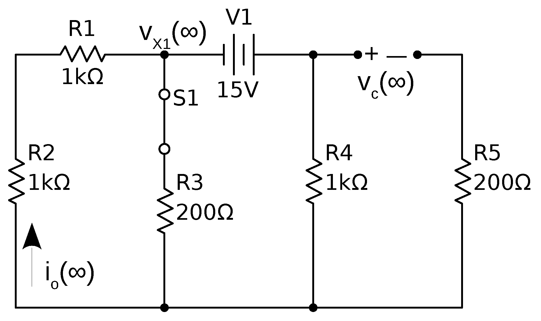
2. Determination of Circuit Response

This section comprises the preliminary work, in which we perform deterministic analysis to derive an expression for the circuit response using basic circuit theorems. To best demonstrate our technique, we use a numerical example of the circuit shown in Figure 1 and find the circuit response in terms of the current i o ( t ) in Figure 1. We use this circuit for ease of demonstration and also due to the fact that the derivation of the probability model of the parameters of other circuit elements can also be explained easily. The demonstrated technique can easily be generalized for a simple RC circuit.
The circuit is previously in a steady state. The circuit enters a transient state when the switch S 1 closes at time t = 0 . Afterward, the circuit returns to a steady state once again. The parameter values of all the circuit components are known as labeled in Figure 1. However, the precise value of the capacitor’s capacitance C is not ascertainable, but it is known to fall within a continuous interval of values. The capacitance can take any of the values in the range with equal probability. After the capacitor takes a capacitance value at random from the interval, the value remains fixed and does not vary during the entire period of the transient response. Therefore, we assume that the capacitance is C farads (F), which is a uniformly distributed continuous random variable. It is to be noted that the capacitance can take on any other probability distribution, such as Gaussian distribution, depending upon the application and reason for its variation. It is also possible that the parameters of more than one circuit element are random variables. In this work, we assume that only the capacitance is a random variable and has continuous uniform distribution.
In Figure 1, a first-order R C circuit is shown. We are interested in the investigation of the response current through the resistor R2. The general form of the current through the resistor R2 is as below:
i o ( t ) = k 1 + k 2 e t τ ,
where k 1 , k 2 and τ are constants, such that
k 1 = i o ( ) ,
k 2 = i o ( 0 ) i o ( ) ,
τ = R e C ,
where i o ( 0 ) represents the initial current at time t = 0 , while i o ( ) represents the current at steady state when t = . The Thevenin equivalent resistance as seen across the capacitor terminals is denoted by R e .
The circuit response in terms of i o ( t ) can be determined using a step-wise approach. Figure 2 depicts the circuit during t < 0 , when the switch has been open for an extended period, allowing the circuit to reach a steady-state condition. The initial voltage v c ( 0 ) across the capacitor before the closure of the switch S 1 is found to be
v c ( 0 ) = v c ( 0 + ) = v c ( 0 ) = 5 V .
The initial current at t = 0 + can be determined by considering the circuit in Figure 3, and is given by
i o ( 0 ) = 65 23 = 2.83 mA .
Similarly, the steady-state current after closing switch S 1 is determined by using Figure 4. This can be calculated to be
i o ( ) = 15 13 = 1.154 mA .
To calculate the circuit time constant using (4), we must initially determine the Thevenin equivalent resistance across the capacitor terminals when the circuit has achieved steady-state status at t > 0 . To determine the Thevenin equivalent resistance, we turn off the independent voltage source V1 in the circuit of Figure 4. The resulting circuit is shown in Figure 5. The Thevenin equivalent resistance R e across the capacitor terminals is obtained as
R e = 4600 13 = 353.85 Ω .
Therefore, the time constant is given by
τ = 353.85 C s .
From (2) and (7), we obtain
k 1 = 15 13 = 1.154 .
Similarly, from (3), (6) and (7), we obtain
k 2 = 65 23 15 13 = 500 299 = 1.67 .
Substituting (9)–(11) in (1), we have
i o ( t ) = 15 13 + 500 299 e t 353.85 C mA ,
which can also be written as
i o ( t ) = 1.154 + 1.67 e t 353.85 C mA .
From (12) and (13), we can note that i o = 65 23 = 2.83 mA at t = 0 , and i o = 15 13 = 1.154 mA at t = . This suggests that the current i o ( t ) recedes during the transient phase, making the transient response in terms of i o ( t ) an exponential decay. It is important to note that the response’s initial and final values at t = 0 and t = do not rely on the capacitance C’s value. Nevertheless, the rapidity with which the response decays, i.e., the time constant, is dependent on the capacitance C. We plot the response in Figure 6 for C = 15 mF.

3. Probability Model

Since the capacitor’s capacitance is merely determined to exist within a range of values, we can use probability techniques to explore the response further. By considering the capacitance as a uniform continuous random variable, the circuit response can be regarded as a random variable that is dependent on the capacitance. In this section, we perform a probabilistic analysis of the circuit response and obtain the probability model in terms of the cumulative distribution function (CDF) and probability density function (PDF) of the current I o .
To explain the notation, we denote a random variable with a capital letter and any of its realizations are represented using the corresponding lower-case letter. Therefore, x is any one of the numerical values of the random variable X.
Suppose we know that the capacitance C lies in a continuous interval ( a , b ) , where b > a > 0 , and each value within the range has the same likelihood of occurrence. In that case, we can treat the capacitance C as a uniform random variable over the interval ( a , b ) . This implies that the probability density function (PDF) f C ( c ) of C can be expressed as follows:
f C ( c ) = 1 b a a c < b , 0 otherwise .
Next, the CDF F C ( c ) is then given by the following:
F C ( c ) = 0 a < c a , c a b a a < c b , 1 a < c > b .
During the interval ( 0 , 5 τ ) , the RC circuit is in the transient state. Consider a time t such that
t = n τ C ,
where the number n fulfills the condition
0 < t 5 τ , 0 < n τ C 5 τ , 0 < n 5 C .
During the transient state, the following relation holds true for the random variable C, with a < c b :
0 < n 5 a .
Using the value of τ from (9) in (16), we obtain
t = n τ C = 353.83 n .
Substituting this value in (12), we obtain an expression for the random variable I o , as below:
I o = 15 13 + 500 299 e n C .
The random variable I o is a derived random variable that depends on the random variable C. From (19), we obtain
500 299 e n C = I o 15 13 ,
C = n ln 299 500 I o 15 13 .
If (20) is to be valid, then I o 15 13 > 0 , i.e., I o > 15 13 . Since C is a uniform random variable over the interval ( a , b ) with b > a > 0 , it can be established that C > 0 . Therefore, the denominator in (20) meets the following condition:
ln 299 500 I o 15 13 < 0 .
As a result, C > 0 .

3.1. Probability Distribution of I o

Now, we will obtain the probability distribution of the random variable I o . For this, we first derive the cumulative distribution function (CDF) F I o ( i o ) , which is given by
F I o ( i o ) = P [ I o i o ] .
The expression I o i o can be evaluated using (19), as below:
15 13 + 500 299 e n C i o ,
n C ln 299 500 i o 15 13 .
We can conclude from (20) and (21) that ln 299 500 i o 15 13 > 0 in (23). Therefore, the reciprocal of (23) gives us the following:
C n ln 299 500 i o 15 13 .
The CDF can now be obtained from (22) and (24), as below:
F I o ( i o ) = P C n ln 299 500 i o 15 13 ,
This gives us the following:
F I o ( i o ) = F C n ln 299 500 i o 15 13 .
Hence, from (15), we obtain the following:
c a b a = n ln 299 500 i o 15 13 a b a ,
c a b a = n ( b a ) ln 299 500 i o 15 13 a b a .
For a complete specification of the CDF F I o ( i o ) , we need to determine three intervals for i o corresponding to c a , a < c b and c > b as is evident from (15). The expressions for these three intervals are derived in the following:
c a
Using (20), we obtain the following:
n ln 299 500 i o 15 13 a ,
i o 15 13 + 500 299 e n a .
Therefore, the interval for F I o ( i o ) corresponding to the interval c a for F C ( c ) is given by (28). We now derive an expression for the interval which corresponds to c > b in the following by using (20):
c > b
n ln 299 500 i o 15 13 > b ,
i o > 15 13 + 500 299 e n b .
Analogously, the expression for the third interval is obtained through the following derivation:
a < c b
a < n ln 299 500 i o 15 13 b ,
15 13 + 500 299 e n a < i o 15 13 + 500 299 e n b .
We can now obtain the complete CDF F I o ( i o ) using (27)–(30), as follows:
F I o ( i o ) = 0 15 13 + 500 299 e n a < i o 15 13 + 500 299 e n a , n ( b a ) ln 299 500 i o 15 13 a b a 15 13 + 500 299 e n a < i o 15 13 + 500 299 e n b , 1 15 13 + 500 299 e n a < i o > 15 13 + 500 299 e n b .
We obtain the PDF by differentiating the CDF in (31):
f I o ( i o ) = n ( b a ) ( i o 15 13 ) ln 299 500 ( i o 15 13 ) 2 .
The PDF f I o ( i o ) can now be completely specified, as below:
f I o ( i o ) = n ( b a ) ( i o 15 13 ) ln 299 500 ( i o 15 13 ) 2 15 13 + 500 299 e n a i o < 15 13 + 500 299 e n b , 0 otherwise .
Either the CDF presented in (31) or the PDF given in (33) provides a complete description of the probability distribution of I o and, consequently, the transient response of the circuit.
With the help of the techniques developed in this section, a probability model of a general RC circuit can be developed in a similar manner starting from (1). In addition, higher-order circuits can also be investigated using a similar approach.

3.2. Validity Check

We can confirm the validity of (33) if the following can be confirmed to hold:
+ f I o ( i o ) d i o = 1 .
Therefore, from (33), we have
+ f I o ( i o ) d i o = 15 13 + 500 299 e n a 15 13 + 500 299 e n b n ( b a ) ( i o 15 13 ) ln 299 500 ( i o 15 13 ) 2 d i o .
This can be solved using substitution. Therefore, let
u = ln 299 500 ( i o 15 13 ) .
From this, we can obtain the following:
d i o = i o 15 13 d u .
By the substitution in (36), we obtain the limits for u in (35) as follows:
u = n a .
u = n b .
Substituting (36) and (37) in (35), and making use of the limits (38) and (39), we obtain
+ f I o ( i o ) d i o = n ( b a ) n a n b d u u 2 ,
+ f I o ( i o ) d i o = n ( b a ) 1 u n a n b = 1 .
Hence, (33) satisfies the condition in (34). Therefore, it is concluded that it is a valid PDF.

3.3. Utilization of the Probability Model

To illustrate the usage of the probability model, we provide an example where we take a = 10 mF and b = 20 mF, resulting in an expected value of C as E [ C ] = 15 mF. By substituting these values into (14) and (15), we acquire the ensuing PDF and CDF of C, respectively.
f C ( c ) = 1 10 10 c < 20 , 0 otherwise ,
F C ( c ) = 0 10 < c 10 , c 10 10 10 < c 20 , 1 10 < c > 20 .
The unit mF for C is used in (42) and (43). In accordance with (17), let us now assume n = a = 10 mF. Therefore, from (18), we obtain t = 353.83 × 10 × 10 3 = 3.538 s. As 10 < c 20 , therefore, using (9), we note that t = 3.538 < τ , which is within the transient state. By substituting a = 10 , b = 20 and n = a = 10 into (31), we can obtain the following CDF:
F I o ( i o ) = 0 1.77 < i o 1.77 , 1 ln 299 500 i o 15 13 1 1.77 < i o 2.17 , 1 1.77 < i o > 2.17 .
Similarly, the PDF for this specific example can be obtained from (33), as below:
f I o ( i o ) = 1 ( i o 15 13 ) ln 299 500 ( i o 15 13 ) 2 1.77 i o < 2.17 , 0 otherwise .
The probability model for the scenario where C∼uniform ( 10 , 20 ) can be obtained from the CDF in (44) and the PDF in (45). In the CDF and the PDF, the unit mA is used for the current i o . The CDF and PDF for this example are plotted in Figure 7 and Figure 8, respectively.
Utilizing the CDF and PDF, probabilities can be calculated for varying values of the current i o , which in turn helps in analyzing the transient response. As an example, let us find P [ I o 2.0 ] . This can be calculated using either the CDF or the PDF. As the former is convenient, we use the CDF from (44) to obtain
P [ I o 2.0 ] = F I o ( 2.0 ) = 0.468 .
Therefore, it can be stated that the probability that i o is below or equal to 2.0 mA at t = 3.538 s is 46.8 % . It can be observed from (44) and (45) that F I o ( i o ) = 0 and f I o ( i o ) = 0 for i o < 1.77 . Therefore, P [ I o 2.0 ] implies P [ 1.77 < I o 2.0 ] . In other words, the probability of i o falling between 1.77 and 2.0 mA is 46.8 % . This also implies that the probability of i o falling between 2.0 and 2.17 mA is 100 46.8 = 53.2 % . All these probability values for this specific example are calculated at time t = 3.538 s, which falls within the transient state. The probability for any other time can be calculated by choosing an appropriate value of n.
The probability models derived in this article can be leveraged for the analysis and investigation of an electric circuit with a failed component. In artificial intelligence and machine learning, probability theory is a key technique [25,26]. Designing an intelligent system that can carry out a desired task after learning from the environment and the data is the goal of artificial intelligence and machine learning applications. Numerous outcomes may be possible while carrying out a task. As a result, the machine learning model uses data to make predictions, approximations and estimations. In carrying out these important processes, probability theory is crucial [27,28,29,30]. The probability models created in our research can also be used to analyze and forecast how a circuit will behave when a component fails.

4. Probability Models of Other Parameters

The probability model for any voltage or current in the circuit can be obtained by following a similar approach used for deriving the probability model of I o . The circuit parameter of interest is represented as a function of C, and its corresponding CDF and PDF are obtained using a similar procedure to that employed for deriving the probability model of I o . Alternatively, if a circuit variable is a function of I o , then its probability distribution can also be determined from the probability model of I o . To further illustrate this methodology, we derive the probability models of the following three parameters of the circuit:
  • Voltage at node V x 1 ;
  • Current I 1 through the resistor R3;
  • Voltage at node V x 2 .

4.1. Voltage V x 1

Let us consider the voltage across the branch containing resistors R 1 and R 2 . We designate this voltage as V x 1 , and it is given by
V x 1 = ( R 1 + R 2 ) I o .
The unit of i o is mA in the CDF (31) and PDF (33); therefore, we can use R 1 + R 2 = 2 k Ω , and
V x 1 = 2 I o .
It is easy to notice that V x 1 is a random variable that is derived from I o and is a constant multiple of I o . Therefore, we can establish the relationships between the CDFs F V x 1 ( v x 1 ) and F I o ( i o ) and the PDFs f V x 1 ( v x 1 ) and f I o ( i o ) as follows:
F V x 1 ( v x 1 ) = P [ V x 1 v x 1 ] ,
Using (48), we have
F V x 1 ( v x 1 ) = P [ 2 I o v x 1 ] ,
F V x 1 ( v x 1 ) = P [ I o > v x 1 2 ] ,
F V x 1 ( v x 1 ) = 1 P [ I o v x 1 2 ] ,
Therefore,
F V x 1 ( v x 1 ) = 1 F I o ( v x 1 2 ) .
Differentiating this, we obtain the PDF as shown below:
f V x 1 ( v x 1 ) = 1 2 f I o ( v x 1 2 ) .
From (31) and (53), we obtain the CDF F V x 1 ( v x 1 ) , as shown below:
F V x 1 ( v x 1 ) = 0 30 13 1000 299 e n b < v x 1 30 13 1000 299 e n b , n ( b a ) ln 299 500 v x 1 2 + 15 13 + b b a 30 13 1000 299 e n b < v x 1 30 13 1000 299 e n a , 1 30 13 1000 299 e n a < v x 1 > 30 13 1000 299 e n a .
In a similar manner, we obtain the PDF f V x 1 ( v x 1 ) from (33) and (54) as follows:
f V x 1 ( v x 1 ) = n 2 ( b a ) ( v x 1 2 + 15 13 ) ln 299 500 ( v x 1 2 + 15 13 ) 2 30 13 1000 299 e n b v x 1 < 30 13 1000 299 e n a , 0 otherwise .

Example for the Probability Model of V x 1

We now demonstrate the usage of the probability model of V x 1 given by (55) and (56). For this, we use the probability model of C as described in (42) and (43). Therefore, a = 10 mF, b = 20 mF and n = a = 10 mF. Substituting these values in (55), we obtain the CDF for our example:
F V x 1 ( v x 1 ) = 0 4.336 < v x 1 4.336 , 1 ln 299 500 v x 1 2 + 15 13 + 2 4.336 < v x 1 3.538 , 1 4.336 < v x 1 > 3.538 .
Similarly, from (56), we obtain the PDF for the specific case, as shown below:
f V x 1 ( v x 1 ) = 1 2 ( v x 1 2 + 15 13 ) ln 299 500 ( v x 1 2 + 15 13 ) 2 4.336 v x 1 < 3.538 , 0 otherwise .
Let us now calculate the probability P [ V x 1 > 4 ] . This can be calculated using either (57) or (58). Using (57), we have
P [ V x 1 > 4 ] = 1 P [ V x 1 4 ] = 1 F V x 1 ( 4 ) = 0.468 .
It is to be noted that v x 1 = 4 V when i o = 2 mA. Therefore, the result in (59) is in harmony with (46). As a further example, let us calculate the probabilities P [ 4 < V x 1 3.7 ] and P [ 4.3 < V x 1 4 ] and compare the results. Again, from (57), we obtain the probabilities as follows:
P [ 4 < V x 1 3.7 ] = F V x 1 ( 3.7 ) F V x 1 ( 4 ) = 0.327 ,
P [ 4.3 < V x 1 4 ] = F V x 1 ( 4 ) F V x 1 ( 4.3 ) = 0.462 .
So, the likelihood of V x 1 falling between 4.3 V and 4 V at time t = 3.538 s, given that C follows a uniform distribution between 10 and 20, is greater than the likelihood of V x 1 falling between 4 V and 3.7 V.

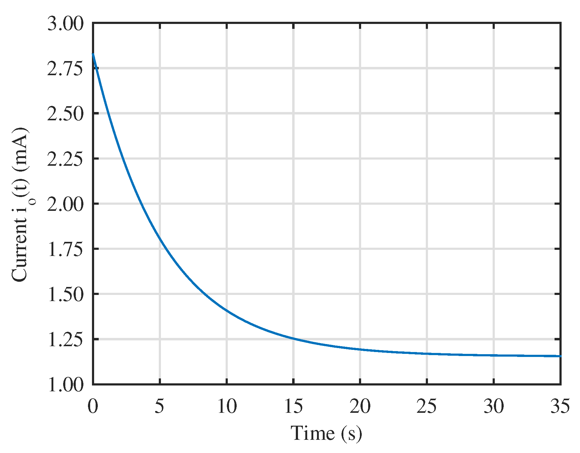
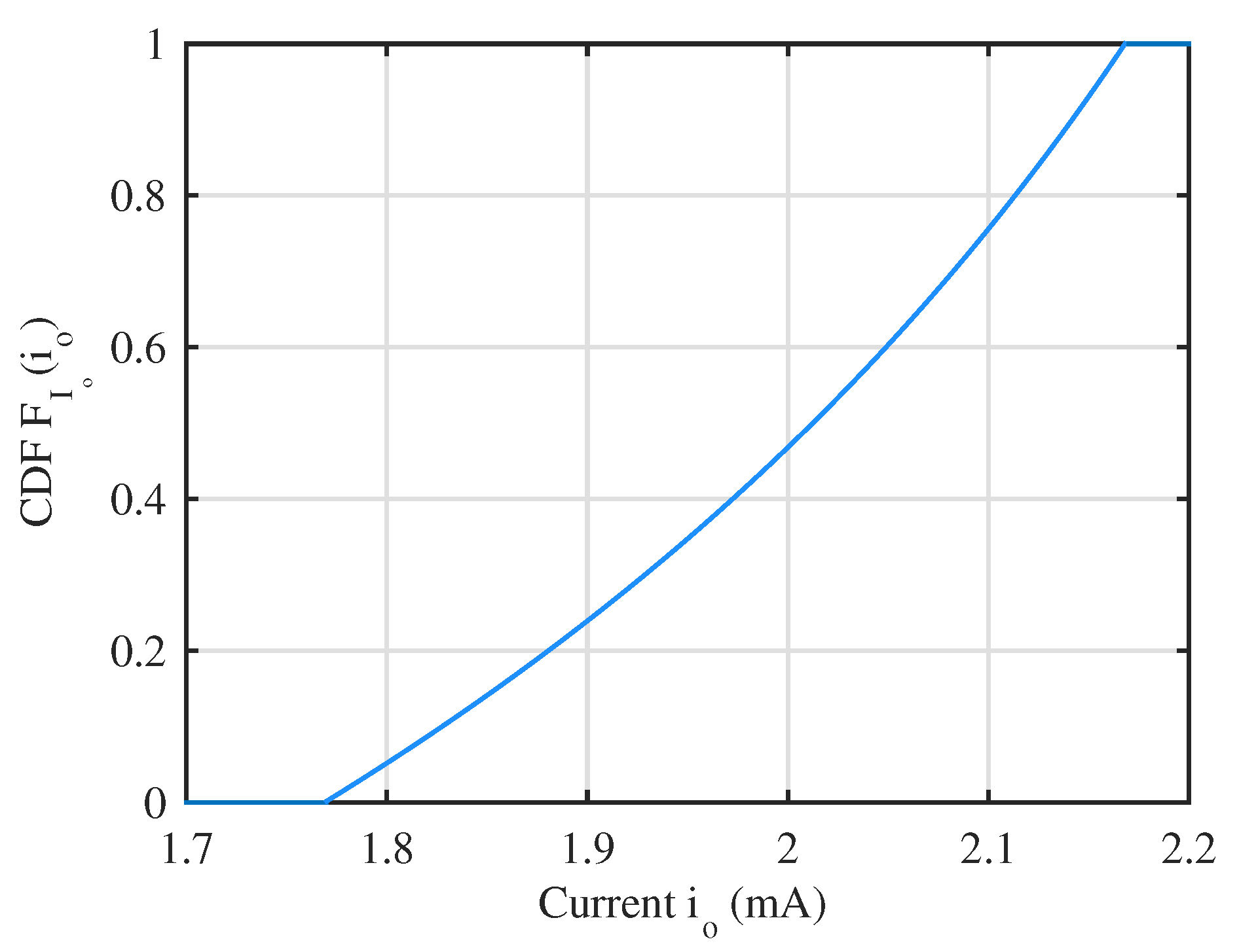
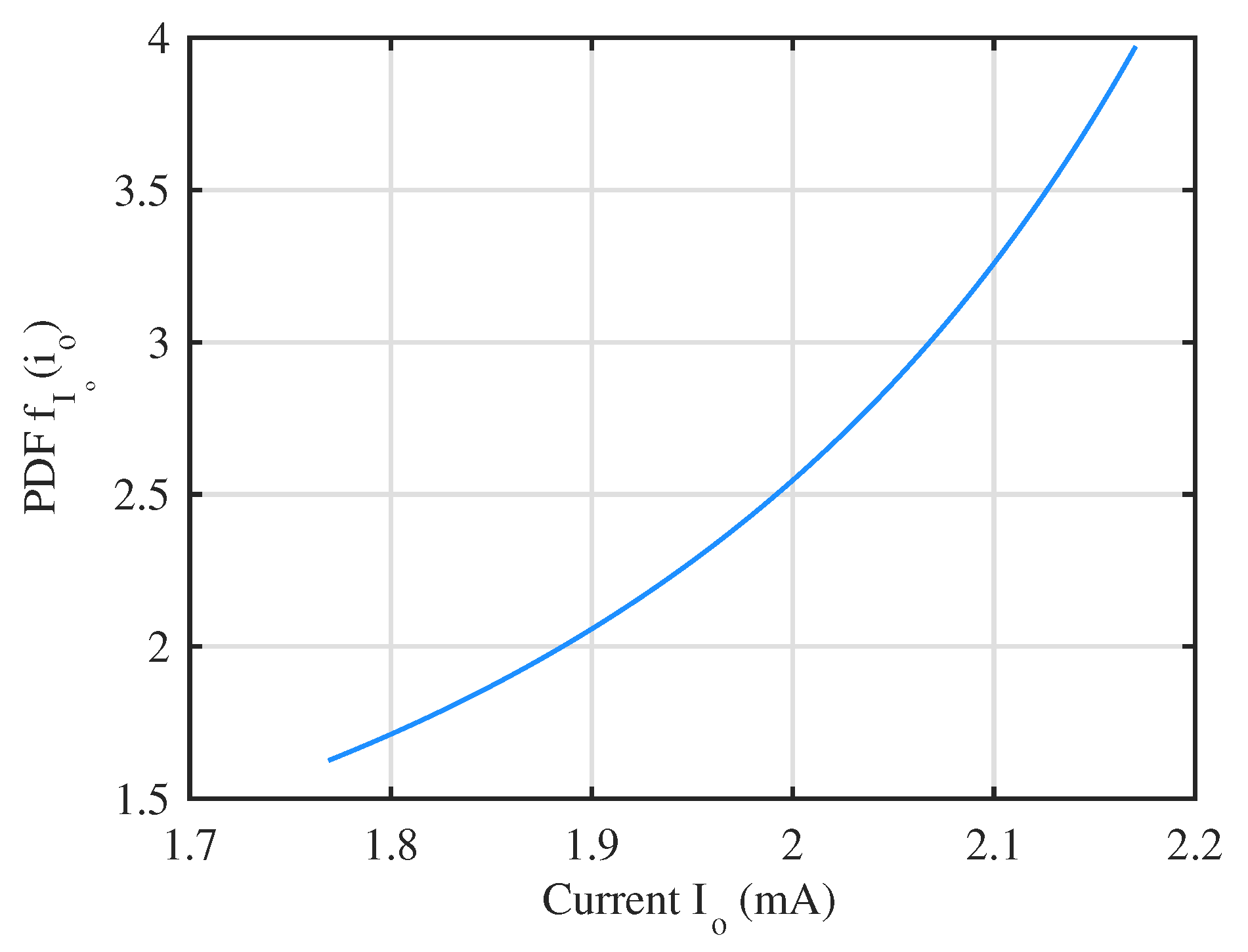
4.2. Current through Resistor R3

We now derive the probability model of the current through the resistor R3 in the direction from the node V x 1 to the bottom node. Let us denote this current using I 1 . The current I 1 is given by
I 1 = V x 1 200 A
To keep the model derived for I o consistent, let us express I 1 also in mA. Therefore,
I 1 = 5 V x 1 mA
This expresses the current I 1 as a function of V x 1 . Therefore, we can leverage the already derived probability model of V x 1 to develop the probability model of I 1 . The CDF F I 1 ( i 1 ) of I 1 is given by
F I 1 ( i 1 ) = P [ I 1 i 1 ] ,
F I 1 ( i 1 ) = P [ 5 V x 1 i 1 ] ,
F I 1 ( i 1 ) = P [ V x 1 i 1 5 ] ,
F I 1 ( i 1 ) = F V x 1 ( i 1 5 ) ,
Differentiating this, we obtain the PDF as follows:
f I 1 ( i 1 ) = 1 5 f V x 1 ( i 1 5 ) ,
From (55) and (68), we obtain the CDF F I 1 ( i 1 ) , as follows:
F I 1 ( i 1 ) = 0 150 13 5000 299 e n b < i 1 150 13 5000 299 e n b , n ( b a ) ln 299 500 i 1 10 + 15 13 + b b a 150 13 5000 299 e n b < i 1 150 13 5000 299 e n a , 1 150 13 5000 299 e n a < i 1 > 150 13 5000 299 e n a .
We can obtain the PDF by differentiating (69) or from (56) and (68) as follows:
f I 1 ( i 1 ) = n 10 ( b a ) ( i 1 10 + 15 13 ) ln 299 500 ( i 1 10 + 15 13 ) 2 150 13 5000 299 e n b i 1 < 150 13 5000 299 e n a , 0 otherwise .

Example for the Probability Model of I 1

For our example, let us assume the values of the parameters a, b and n are the same as those used previously, i.e., a = 10 mF, b = 20 mF and n = a = 10 . Therefore, the probability model of C is the same as that given by (42) and (43). We obtain the CDF for this example by substituting the values of the parameters a, b and n in (69) as follows:
F I 1 ( i 1 ) = 0 21.681 < i 1 21.681 , 1 ln 299 500 i 1 10 + 15 13 + 2 21.681 < i 1 17.690 , 1 21.681 < i 1 > 17.690 .
Similarly, using the parameter values in (70), we obtain the PDF as follows:
f I 1 ( i 1 ) = 1 10 ( i 1 10 + 15 13 ) ln 299 500 ( i 1 10 + 15 13 ) 2 21.681 i 1 < 17.690 , 0 otherwise .
Using either the CDF in (71) or the PDF in (72), we can obtain the probability for a specific range of the current I 1 . For example, we obtain P [ I 1 19 ] from the PDF as follows:
P [ I 1 19 ] = 21.681 19 f I o ( i o ) d i o = 0.761 ,
We can also solve this using the CDF, as P [ I 1 19 ] = F I 1 ( 19 ) = 0.761 .

4.3. Voltage V x 2

Considering the voltage relationships in Figure 3, it can be readily observed that the voltage V x 2 is given by
V x 2 = V x 1 + 15 .
Therefore, we can once again leverage the already derived probability model of V x 1 to develop the probability model of V x 2 . The CDF F V x 2 is given by
F V x 2 ( v x 2 ) = P [ V x 2 v x 2 ] ,
F V x 2 ( v x 2 ) = P [ V x 1 + 15 v x 2 ] ,
F V x 2 ( v x 2 ) = P [ V x 1 v x 2 15 ] ,
F V x 2 ( v x 2 ) = F V x 1 ( v x 2 15 ) .
Differentiating this, we obtain the relationship for the PDF f V x 2 ( v x 2 ) as follows:
f V x 2 ( v x 2 ) = f V x 1 ( v x 2 15 ) .
From (55) and (78), the CDF F V x 2 ( v x 2 ) is obtained as follows:
F V x 2 ( v x 2 ) = 0 165 13 1000 299 e n b < v x 2 165 13 1000 299 e n b , n ( b a ) ln 299 1000 v x 2 165 13 + b b a 165 13 1000 299 e n b < v x 2 165 13 1000 299 e n a , 1 165 13 1000 299 e n a < v x 2 > 165 13 1000 299 e n a .
We obtain the PDF f V x 2 ( v x 2 ) from (56) and (79) as follows:
f V x 2 ( v x 2 ) = n ( b a ) ( v x 2 165 13 ) ln 299 1000 ( v x 2 165 13 ) 2 165 13 1000 299 e n b v x 2 < 165 13 1000 299 e n a . 0 otherwise .

Example for the Probability Model of V x 2

As used in the examples for V x 1 and I 1 , we now substitute the same values of the parameters, i.e., a = 10 mF, b = 20 mF and n = a = 10 in (80) and (81) to obtain the CDF and the PDF, respectively, for the example for V x 2 as follows:
F V x 2 ( v x 2 ) = 0 10.664 < v x 2 10.664 , 1 ln 299 1000 v x 2 165 13 + 2 10.664 < v x 2 11.462 , 1 10.664 < v x 2 > 11.462 .
f V x 2 ( v x 2 ) = 1 ( v x 2 165 13 ) ln 299 1000 ( v x 2 165 13 ) 2 10.664 v x 2 < 11.462 . 0 otherwise .
For further demonstration, let us now calculate the probability, say, P [ V x 2 11 ] , using the CDF in (82) as follows:
P [ V x 2 11 ] = F V x 2 ( 11 ) = 0.532
We can calculate the same probability using the PDF in (83) as follows:
P [ V x 2 11 ] = 10.664 11 f V x 2 ( v x 2 ) d v x 2 = 0.532 ,
To summarize, the probability model of a circuit parameter provided by the CDF and the PDF can be developed directly or it can be obtained from an already derived model of another parameter. The probability model can then used for the probability estimation of circuit parameters.

5. Conclusions

In this work, we have conducted an investigation into the exponentially decaying transient response of an RC electric circuit. The capacitance of the circuit’s capacitor is subject to uncertainty, with its true value only known to exist within a range. To account for this, we have treated the capacitance as a continuous uniform random variable. Utilizing conventional analysis techniques, we have derived a general expression for the circuit’s transient response as a function of the capacitance. Subsequently, we have applied probability methods to establish a probability model for the circuit’s decaying transient response in terms of a branch current, which has been further utilized to derive the probability distribution of the branch voltage. These models have been utilized to perform a probabilistic analysis of the RC circuit’s decaying transient response. In future work, we aim to extend our analysis to consider more than one circuit parameter as random variables and consider employing other distributions in the derivation of the probability model. We also plan to derive probability models of general first-order and higher-order circuits using the techniques developed in this work.

Author Contributions

Conceptualization, M.F.-i.-A.; methodology, M.F.-i.-A. and A.S.; validation, M.F.-i.-A., Z.H.K. and A.G.; investigation, A.G.; resources, Z.H.K. and A.G.; writing—original draft preparation, M.F.-i.-A.; writing—review and editing, M.F.-i.-A., A.S. and A.G.; visualization, A.G.; supervision, M.F.-i.-A.; project administration, Z.H.K. and A.G. All authors have read and agreed to the published version of the manuscript.

Funding

This research received no external funding.

Institutional Review Board Statement

Not applicable.

Informed Consent Statement

Not applicable.

Data Availability Statement

Not applicable.

Conflicts of Interest

The authors declare no conflict of interest.

References

  1. Zheng, S.; Kang, Z.; Li, L.; Zhang, A.; Zhao, K.; Zhou, Y. Influence of series RC circuit parameters on the streamer discharge process of gas spark switch. Vacuum 2021, 193, 110518. [Google Scholar] [CrossRef]
  2. Qureshi, S.; Chang, M.M.; Shaikh, A.A. Analysis of series RL and RC circuits with time-invariant source using truncated M, Atangana beta and conformable derivatives. J. Ocean. Eng. Sci. 2021, 6, 217–227. [Google Scholar] [CrossRef]
  3. Wang, K.J.; Sun, H.C.; Fei, Z. The transient analysis for zero-input response of fractal RC circuit based on local fractional derivative. Alex. Eng. J. 2020, 59, 4669–4675. [Google Scholar] [CrossRef]
  4. Zhu, Q.; Zhou, M.; Qiao, Y.; Wu, N.; Hou, Y. Multiobjective Scheduling of Dual-Blade Robotic Cells in Wafer Fabrication. IEEE Trans. Syst. Man Cybern. Syst. 2020, 50, 5015–5023. [Google Scholar] [CrossRef]
  5. Koo, J.; Kim, B.; Park, H.J.; Sim, J.Y. A Quadrature RC Oscillator With Noise Reduction by Voltage Swing Control. IEEE Trans. Circuits Syst. Regul. Pap. 2019, 66, 3077–3088. [Google Scholar] [CrossRef]
  6. Sevilmiş, F.; Karaca, H. An advanced hybrid pre-filtering/in-loop-filtering based PLL under adverse grid conditions. Eng. Sci. Technol. Int. J. 2021, 24, 1144–1152. [Google Scholar] [CrossRef]
  7. Li, C.; Chen, S.; Luo, H.; Li, C.; Li, W.; He, X. A Modified RC Snubber with Coupled Inductor for Active Voltage Balancing of Series-Connected SiC MOSFETs. IEEE Trans. Power Electron. 2021, 36, 11208–11220. [Google Scholar] [CrossRef]
  8. Ebrahim, M.A.; Elyan, T.; Wadie, F.; Abd-Allah, M.A. Optimal design of RC snubber circuit for mitigating transient overvoltage on VCB via hybrid FFT/Wavelet Genetic approach. Electr. Power Syst. Res. 2017, 143, 451–461. [Google Scholar] [CrossRef]
  9. Momeni, M.; Moezzi, M. A Low Loss and Area Efficient RC Passive Poly Phase Filter for Monolithic GHz Vector-Sum Circuits. IEEE Trans. Circuits Syst. II Express Briefs 2019, 66, 1134–1138. [Google Scholar] [CrossRef]
  10. Merlo, L.; Di Biccari, L.; Cerati, L.; Andreini, A. Design of RC trigger circuit for dynamically activated ESD protections ensuring application requirements and ESD performances. Microelectron. Reliab. 2022, 138, 114685. [Google Scholar] [CrossRef]
  11. Ding, C.; Nie, T.; Tian, X.; Chen, T.; Yuan, Z. Analysis of the influence of RC buffer on DC solid-state circuit breaker. Energy Rep. 2020, 6, 1483–1489. [Google Scholar] [CrossRef]
  12. Chen, J.; Luo, Q.; Huang, J.; He, Q.; Sun, P.; Du, X. Analysis and Design of an RC Snubber Circuit to Suppress False Triggering Oscillation for GaN Devices in Half-Bridge Circuits. IEEE Trans. Power Electron. 2020, 35, 2690–2704. [Google Scholar] [CrossRef]
  13. Dou, G.; Zhang, Y.; Yang, H.; Han, M.; Guo, M.; Gai, W. RC Bridge Oscillation Memristor Chaotic Circuit for Electrical and Electronic Technology Extended Simulation Experiment. Micromachines 2023, 14, 410. [Google Scholar] [CrossRef] [PubMed]
  14. Wan, F.; Gu, T.; Ravelo, B.; Li, B.; Cheng, J.; Yuan, Q.; Ge, J. Negative Group Delay Theory of a Four-Port RC-Network Feedback Operational Amplifier. IEEE Access 2019, 7, 75708–75720. [Google Scholar] [CrossRef]
  15. Lavalle-Aviles, F.; Sánchez-Sinencio, E. A 0.6-V Power-Efficient Active-RC Analog Low-Pass Filter with Cutoff Frequency Selection. IEEE Trans. Very Large Scale Integr. Syst. 2020, 28, 1757–1769. [Google Scholar] [CrossRef]
  16. Cheong, H.G.; Kim, Y.S.; Chu, C.N. Machining Characteristics of an RC-type Generator Circuit With an N-channel MOSFET in Micro EDM. Procedia CIRP 2018, 68, 631–636. [Google Scholar] [CrossRef]
  17. Wu, S.L.; Al-Khaleel, M. Convergence analysis of the Neumann–Neumann waveform relaxation method for time-fractional RC circuits. Simul. Model. Pract. Theory 2016, 64, 43–56. [Google Scholar] [CrossRef]
  18. Farooq-i-Azam, M.; Farooq, M.O. Probability model of the exponentially rising transient response of a failed RC circuit. Eng. Fail. Anal. 2022, 142, 106770. [Google Scholar] [CrossRef]
  19. Farooq-i-Azam, M.; Khan, Z.H.; Hassan, S.R.; Asif, R. Probabilistic Analysis of an RL Circuit Transient Response under Inductor Failure Conditions. Electronics 2022, 11, 4051. [Google Scholar] [CrossRef]
  20. Yu, W.; de la Rosa, E. Neural Modeling with Guaranteed Input-Output Probability Distributions. IEEE Trans. Syst. Man Cybern. Syst. 2020, 51, 6660–6668. [Google Scholar] [CrossRef]
  21. Seliem, H.; Shahidi, R.; Ahmed, M.H.; Shehata, M.S. Accurate Probability Distribution Calculation for Drone-Based Highway-VANETs. IEEE Trans. Veh. Technol. 2020, 69, 1127–1130. [Google Scholar] [CrossRef]
  22. Bahri, Z. Asymptotic series expansion for the probability density function of the interference due to Faster-Than-Nyquist signaling. Eng. Sci. Technol. Int. J. 2017, 20, 1507–1514. [Google Scholar] [CrossRef]
  23. Singh, K.K.; Yadav, P.; Singh, A.; Dhiman, G.; Cengiz, K. Cooperative spectrum sensing optimization for cognitive radio in 6 G networks. Comput. Electr. Eng. 2021, 95, 107378. [Google Scholar] [CrossRef]
  24. Quan, Q.; Cui, G.; Du, G.X. Controllable probability and optimization of multicopters. Aerosp. Sci. Technol. 2021, 119, 107162. [Google Scholar] [CrossRef]
  25. Abdul Majid, A. Forecasting Monthly Wind Energy Using an Alternative Machine Training Method with Curve Fitting and Temporal Error Extraction Algorithm. Energies 2022, 15, 8596. [Google Scholar] [CrossRef]
  26. Ghahramani, Z. Probabilistic machine learning and artificial intelligence. Nature 2015, 521, 452–459. [Google Scholar] [CrossRef] [PubMed]
  27. Anthony, M. Probability Theory in Machine Learning. In Encyclopedia of the Sciences of Learning; Seel, N.M., Ed.; Springer: Boston, MA, USA, 2012; pp. 2677–2680. [Google Scholar] [CrossRef]
  28. Ranftl, S. A Connection between Probability, Physics and Neural Networks. Phys. Sci. Forum 2022, 5, 11. [Google Scholar] [CrossRef]
  29. Murphy, K.P. Probabilistic Machine Learning: An Introduction; MIT Press: Cambridge, MA, USA, 2022. [Google Scholar]
  30. Murphy, K.P. Probabilistic Machine Learning: Advanced Topics; MIT Press: Cambridge, MA, USA, 2023. [Google Scholar]
Figure 1. Response of the RC electric circuit is examined once the switch S 1 is closed at time t = 0 . The precise value of the capacitor’s capacitance is unknown, except for the fact that it is restricted to a specific fixed interval of values.
Symmetry 15 01378 g001
Figure 2. Prior to t = 0 , the switch S 1 had been open for a considerable amount of time, causing the circuit to settle into a steady state. At this point, the capacitor is fully charged and the voltage across the charged capacitor is v c ( 0 ) .
Symmetry 15 01378 g002
Figure 3. At t = 0 + when the switch S1 is closed. The circuit is depicted in the figure. The capacitor has been substituted with a voltage source, the voltage of which is equivalent to the initial voltage of the capacitor.
Symmetry 15 01378 g003
Figure 4. Once the switch S 1 is closed, and ample time has elapsed, the circuit attains a steady-state status at t > 0 , as shown in the figure. The capacitor is now charged to a different value.
Symmetry 15 01378 g004
Figure 5. Circuit at t > 0 after turning off voltage source V1 for the calculation of the Thevenin resistance across the capacitor terminals.
Symmetry 15 01378 g005
Figure 6. The plot illustrates the transient response with a capacitance value of 15 mF. At t = 0 , the initial current i o is 2.83 mA, whereas at t = , it decreases to 1.154 mA. The current i o ( t ) displays an exponential decay from t = 0 to t = .
Symmetry 15 01378 g006
Figure 7. The cumulative distribution function (CDF) F I o ( i o ) when a = 10 mF, b = 20 mF and C is a uniform random variable over the interval ( a , b ) .
Symmetry 15 01378 g007
Figure 8. The probability density function (PDF) f I o ( i o ) when a = 10 mF, b = 20 mF and C is uniform ( a , b ) random variable.
Symmetry 15 01378 g008
Disclaimer/Publisher’s Note: The statements, opinions and data contained in all publications are solely those of the individual author(s) and contributor(s) and not of MDPI and/or the editor(s). MDPI and/or the editor(s) disclaim responsibility for any injury to people or property resulting from any ideas, methods, instructions or products referred to in the content.

