Abstract
The most important advantage of conjugate gradient methods (CGs) is that these methods have low memory requirements and convergence speed. This paper contains two main parts that deal with two application problems, as follows. In the first part, three new parameters of the CG methods are designed and then combined by employing a convex combination. The search direction is a four-term hybrid form for modified classical CG methods with some newly proposed parameters. The result of this hybridization is the acquisition of a newly developed hybrid CGCG method containing four terms. The proposed CGCG has sufficient descent properties. The convergence analysis of the proposed method is considered under some reasonable conditions. A numerical investigation is carried out for an unconstrained optimization problem. The comparison between the newly suggested algorithm (CGCG) and five other classical CG algorithms shows that the new method is competitive with and in all statuses superior to the five methods in terms of efficiency reliability and effectiveness in solving large-scale, unconstrained optimization problems. The second main part of this paper discusses the image restoration problem. By using the adaptive median filter method, the noise in an image is detected, and then the corrupted pixels of the image are restored by using a new family of modified hybrid CG methods. This new family has four terms: the first is the negative gradient; the second one consists of either the HS-CG method or the HZ-CG method; and the third and fourth terms are taken from our proposed CGCG method. Additionally, a change in the size of the filter window plays a key role in improving the performance of this family of CG methods, according to the noise level. Four famous images (test problems) are used to examine the performance of the new family of modified hybrid CG methods. The outstanding clearness of the restored images indicates that the new family of modified hybrid CG methods has reliable efficiency and effectiveness in dealing with image restoration problems.
1. Introduction
CG parameters are widely utilized for dealing with a great variety of different optimization problems.
Many researchers have focused on modifying CG parameters in order to augment the corresponding CG strategies. Those newly proposed approaches have enhanced the performance of the conventional CG methods.
The CG algorithm has been applied numerous areas such as neural networks, image processing, medical science, operational research, engineering problems, etc.
Thus, the different problems generated in these applications can be formulated in various forms, such as unconstrained, constrained, multi-objective optimization problems, nonlinear systems, etc.
Therefore, this study concentrates on an unconstrained optimization problem defined as
where the function is continuously differentiable. CG methods have very powerful convergence abilities and fair storage needs.
Among the most important advantages of the CG method are its low memory requirements and convergence speed [1].
Thus, many authors have analyzed CG methods in order to solve large minimization optimization problems and other applications [2].
Accordingly, many authors have suggested several modificationsof the classical methods that deal with optimization problems, e.g, the Newton method [3], the quasi-Newton method [4], the semi-gradient method [5], the hybrid gradient meta-heuristic algorithm [6,7], and the CG-method [8,9,10,11].
Different versions of the Newton method are widely employed to solve multiple different optimization problems because of their fast convergence rates, e.g., [12,13,14,15,16,17].
However, these methods are very expensive since they require a calculation of the exact or approximate Jacobian matrix for each iteration. Therefore, it is best to avoid utilizing these methods when solving large-scale optimization problems.
Hence, the use of the CG technique has been more widespread compared to other conventional methods because of its simplicity, lower storage requirements, efficiency, and optimal convergence features [1,18,19].
Accordingly, the reason for selecting this topic for analysis depends on the following bases.
Conjugate gradient methods (CGs) are associated with a very strong global convergence theory for a local minimizer and they have low memory requirements. Moreover, in practice, combining the CG method with a line search strategy showed merit in dealing with an unconstrained minimization problem [20,21,22,23,24,25].
Additionally, CG parameters have shown remarkable superiority in solving problems involving systems of nonlinear equations (see, for example, [26,27,28,29,30,31,32,33,34,35]). According to previous successful uses of CG techniques to solve different applications problems, many authors have adapted CG methods such that they are capable of dealing with image restoration problems (see, for example, [25,35,36,37,38,39,40,41,42,43]).
Many researchers have shown that the CG method can also be used as a mathematical tool for training deep neural networks. (see, for example, [44,45,46,47,48]).
Generally, the iterative formula used to generate the sequence solutions of Problem (1) is defined in the following form
where is the current point, is the step size obtained using a line search technique, and is the search direction decided by the conjugate parameter .
The sequence of the step size and the search direction can be generated through various approaches. These approaches depend on many concepts that have been implemented for designing different formulas of , , and .
The short and simple formula used to determinethe search direction is defined as follows:
where , is known as the CG parameter and represents the gradient vector of the function f at .
A core difference between all the proposed CG methods is the form of the parameter .
The proposal of new CG parameters of the classical CG methods has led to improvements in said methods’ performance in dealing with many problems in different applications.
The classical CG methods include the HS-CG method proposed by the authors of [9]; the FR-CG parameter proposed by the authors of [8]; the PRP-CG method proposed by Polak and Ribiere [11], Polyak [49]; the LS-CG method proposed by Liu and Storey [10]; and the DY-CG method proposed by Dai and Yuan [50]. The value of these CG algorithms contains one term.
These CG parameters are listed in the following formulas:
where .
where is the Euclidean norm and the values of the parameter are computed as follows: .
Recently, many novel formulas for determining the parameter have been suggested, with those corresponding to CG methods including two or three terms (see [21,22,25,51,52])
In several papers, CG methods studied using convergence analysis have been reported (see [42,53]).
For example, Hager and Zhang [54] presented the following CG-method, which contains three terms:
where , .
In their numerical experiments, the authors of [54] set .
If employed appropriately, remarkable results can be when obtained using the CG method to solve the many different problems posed in several applications.
Hence, the modifications and additions to and recommendations for conventional CG techniques are undertaken to develop an updated version of the CG method or a novel technique with widespread applications.
These propositions and modifications have either one term or multiple terms.
For example, Jiang et al. [25] recently proposed a family of combination 3-term CG techniques for solving nonlinear optimization problems and aiding image restoration.
The authors of [25] combined the parameter with each parameter in the set to obtain a family of CG methods. They define the direction as follows:
where and . The authors of [25] used the convex combination technique developed by [35]. In addition to their proposal in Formula (10), they have suggested a new CG parameter, which was defined as follows:
where . Then, they combined their new parameter with the parameter to get a new algorithm that solves Problem (1) and can be used in image restoration; furthermore, they performed a convergence analysis of this family of combination 3-term CG methods.
Huo et al. [55] proposed a new CG method containing three parameters in order to solve Problem (1). Moreover, under reasonable assumptions, the author of [55] established the global convergence of their method.
Tian et al. [56] suggested a new hybrid three-term CG approach without using a line search method. The authors of [56] designed the new hybrid descent three-term direction in the following form:
where, when is met, the stopping criterion is satisfied, and the optimal solution is obtained. They proceeded to provide some remarks regarding their proposed directions. In addition, the authors of [56] successfully performed a convergence analysis of their newly proposed CG method (under certain conditions). The numerical outcomes demonstrate that the three-term CG method is more efficient and reliable in terms of solving large-scale unconstrained optimization problems compared to other methods.
Jian et al. [57] proposed a new spectral SCGM approach, i.e., the core study of the authors in [57], which consisted of designing a spectral parameter and a conjugate parameter using the SCGM method. They proved the global convergence of the suggested SCGM method. The approach proposed by the authors of [57] for yielding the spectral parameter is as follows:
The authors clearly showed that when the prior is in a descent.
In addition, they proposed a new conjugate parameter, which was defined as follows:
Subsequently, they presented a convergence-analysis-based proof of the SCGM method. Using the SCGM method, the authors of [57] solved an unconstrained optimization problem with many dimensions.
There are other studies that employ the same convex combination concept with different combination parameters (see, for example, [58]).
Yuan et al. [52] proposed a research direction of the CG method containing the following formula:
where the authors in [52] defined the parameter as follows:
where is a constant. The authors of [52] presented a convergence analysis proof of with some conditions.
Abubakar et al. [20] proposed the following CG-method (a new modified LS method (NMLS)):
where is defined as follows
where , and the parameter is defined by (7) and is defined by
The convergence analysis of this method was carried out by Abubakar et al. [20]. In addition, the numerical results, which were obtained by solving the corresponding unconstrained minimization problems, were implemented in applications in motion control
Alhawarat et al. [59] proposed a new CG method that depends on a convex group between two various search directions of the CG method; then, they employed this method to solve an unconstrained optimization problem involving image restoration. Their proposed method presented incredible results. The numerical results of the method proposed in [59] show that the convex combination allows the new CG method to provide more efficient results than the other compared methods.
Therefore, the convex combination technique plays a critical role in improving the performance of any new version of a CG method. The above arguments indicate that merging two or more parameters of the classical CG methods offers promising results.
Accordingly, such promising results encouraged us to continue this pattern of improving the performance of the classical CG techniques.
Many modifications and performance enhancements of the CG parameters have recently been proposed by numerous authors. Such recently developed GC parameters include two terms: the first one denotes the negative gradient vector, while the second term indicates the parameter proposed by the cited authors (see, for example, [21,22,25].
A brief review of the ideas presented in the literature has inspired us to design a new convex hybrid CG technique. This new convex combined technique has four terms, the first of which is a negative gradient vector, while the other three terms are the proposed parameters multiplied by .
Therefore, the major contributions of this paper include the following aspects.
- The presentation of some suggestions for and modifications to some classical CG parameters with new parameters;
- Three new parameters for CG techniques, which are are combined together, where ;
- Through the above procedures, a new suggested CG approach has been designed, which we dubbed “Convex Group Conjugated Gradient”, which has been shortened to CGCG;
- The performance of a convergence analysis of the new CGCG approach;
- Numerical investigations are offered, which were executed by solving a set of test minimization problems;
- The adaptation of the CGCG algorithm yielded a family of modified CG methods that can be used to deal with image restoration problems;
- By applying the adaptive median filter method, the noise in an image is detected;
- According to the noise level in the corrupted image, a change in the size of the filter window is considered for improving the performance of this family of CG methods;
- Four corrupted images (test problems) with salt-and-pepper noise (at 30–90% levels) are used to examine the performance of the new family of modified hybrid CG methods.
The rest of the current study is arranged as follows. In the next section, the CGCG method and convergence analysis proof are presented. Section 3 presents the numerical experiments concerning the set of optimization test problems solved using the CGCG method and five other traditional CG methods.
Section 4 offers a brief discussion about image processing, including some applications of the adaptive CGCG method (a member of the family of CG methods) in image restoration. Section 5 presents the numerical experiments conducted with the proposed family of CG methods, which concern the solution to an image restoration problem. The last section provides some concluding remarks.
2. CGCG Method
The proposed CGCG method involves modifications to and suggestions for several classical CG-methods, which are listed in (4)–(8). In addition, this CGCG method contains new parameters, which are presented in this paper.
Therefore, the details of the newly proposed CGCG-method are listed in Algorithm 1 and used to solve Problem (1). The convergence analysis proof of the CGCG algorithm is also presented in this section. In addition, the CGCG method is adapted and modified in order to yield the family of CG-methods listed in Algorithms 2–4. These algorithms can be used in image restoration problems, as we will see in Section 4.
| Algorithm 1 A Convex Group Conjugated Gradient Method (CGCG). |
| Input:
, , and , , an initial point and . Output: is the optimal solution. 1: Set and . 2: while . do 3: Compute to fulfill (31) and (32). 4: Calculate a new point . 5: Compute , 6: Set . 7: end while 8: return , the optimal solution. |
| Algorithm 2 CGCG-HS2 Algorithm |
| Step 1: Inputs: Original image (O_img), Noise Ratio(N.R), and W_max . Step 2: Destroy the original (O_img) by using noise (salt and pepper) to obtain a noised image (N_img). Step 3: Apply adaptive median filter algorithm (A.M.F .A) for each level and W_max. Step 4: Detect pixels of the noised image (N_img). Step 5: Use Formulas (53) and (55) to remove the Noise from the corrupted pixels. Step 6: Output: Repaired Image (R_img) (O_img) |
| Algorithm 3 CGCG-HS1 Algorithm |
| Step 1: Inputs: Original image (O_img), Noise Ratio(N.R), and W_max . Step 2: Destroy the original (O_img) using a high noise level (salt and pepper) to obtain a noised image (N_img). Step 2a: If N.R . Step 2b: Set . Step 2b: Otherwise, set . Step 3: Apply adaptive median filter algorithm (A.M.F .A) for each level W_max . Step 4: Detect noisy pixels in the noised image (N_img). Step 5: Use Formulas (53) and (55) to remove the noise from the corrupted pixels. Step 6: Output: Repaired Image (R_img) (O_img) |
| Algorithm 4 CGCG-HZ Algorithm |
| Step 1: Inputs: Original image (O_img), Noise Ratio(N.R), and W_max . Step 2: Destroy the original (O_img) using a high noise level (salt and pepper) to obtain a noised image (N_img). Step 2a: If N.R . Step 2b: Set . Step 2b: Otherwise, set . Step 3: Apply adaptive median filter algorithm (A.M.F .A) for each level with W_max . Step 4: Noisy pixels of the Noise image (N_img) are detected. Step 5: Use Formulas (53) and (56) to remove the Noise from the corrupted pixels. Step 6: Output: Repaired Image (R_img) (O_img) |
Thus, to solve Problem (1), the next iterative form is utilized to generate a new candidate solution:
where is the current point and is the step size in the search direction .
The new proposed CG approach is defined in the following paragraph.
To achieve the global convergence of a hybrid CG technique, one must choose the step length carefully. Additionally, the selection of a suitable search direction must be considered.
The purpose of this procedure is to guarantee that the following sufficient descent condition is satisfied:
for .
Consequently, the following fundamental property is called an angle property. This property and other proposed parameters are critical in developing the proposed method:
where the angle is between and .
Hence, we benefit by obtaining the value of , which will be used to design a new mixed CG method containing four terms. The three terms that represent the core of our proposed method are inspired by the classical conjugate gradient parameters, which are defined in Formulas (4)–(8).
Therefore, we connect the three terms using the following parameter:
In addition, we define the following parameter to represent an option for the CG parameter.
where , are fixed real numbers such that and is an integer.
Then, the three CG parameters are defined as follows:
where
where
where is a fixed number,
where
where , , at the iteration k and n indicates the number of variables of a test problem.
According to the above relations and formulas, the new search direction is defined as follows:
Thus, the newly proposed CG approach includes four terms; we name this suggested method “Convex Group Conjugated Gradient”, which is abbreviated as (CGCG).
To render the CGCG method globally convergent, we use the following line search technique:
and
where and are constants.
According to the search direction (30) and the Wolfe conditions (31) and (32), we present the explicit steps of the (CGCG) technique, as follows.
Now, we present some numerical facts relating to the above parameters, allowing us to discuss the global convergence and descent properties of the CGCG method.
The purpose of the following remark is to facilitate the convergence analysis proof of the CGCG method.
Remark 1.
When both sides of (30) are multiplied by the , we obtain the following:
Then, the fourth term of (33) satisfies the following inequality for each iteration k:
Since , and if the first branch of (28) is satisfied, then ; otherwise, since and it is clear that .
The third term of (33) can be reformulated as follows:
The second term of (33) can be reformulated as follows:
We set the second term of Formula (35) as follows:
The following inequality is applied to the first expression of the numerator, with , .
Then,
then,
Similarly, the second branch of Formula (36) is rewritten as follows:
Therefore,
Note: As we have mentioned above, the four results that are listed in Formulas (34)–(38) of Remark 1 are applied in the convergence analysis of the suggested method described in Section 2.
The convergence analysis and descent property of the CGCG technique are presented in the following section.
2.1. Convergence Analysis
The convergence analysis of Algorithm 1 is presented as follows. First, two useful hypotheses are listed as follows.
Hypothesis 1.
Let a function be continuously differentiable.
Hypothesis 2.
In a few neighborhoods N of the level group, , the gradient vector of the function is Lipschitz-continuous.
Therefore, there is a fixed that satisfies the following inequality , .
The following lemma shows that the search direction defined by Formula (30) is a descent direction.
Lemma 1.
Let be the sequence obtained using Algorithm 1. If ; then,
where .
Proof.
According to (34) and Remark 1, the following cases exist that can be used to prove that Formula (39) is true.
Then,
where .
Therefore, (39) is met.
Case II: When and , then Formula (33) is as follows.
we set , with . Then,
where . Therefore, (39) is met.
Then,
where ; thus, (39) is met.
Then,
where ; thus, (39) is met.
Hence, the above four cases show that (39) is true. □
Below, some hypotheses and a useful lemma are presented, where the obtained result was essentially proven by the author of [60] and the author of [61,62].
Lemma 2.
Let be a starting point that satisfies Hypothesis 1. Regard any algorithm to be of Form (18), such that the satisfies (19) and the satisfies conditions (31) and (32).
Hence, the following inequality is met.
Theorem 1.
Suppose that Hypotheses 1 and 2 are met and that the following is satisfied: . Then, the sequence generated using the CGCGC method satisfies the next result.
Proof.
Proof by contradiction: assume that (45) is incorrect; hence, for some .
Then, the next result is correct.
Computational Cost Analysis of CGCG Method
In general, any modified version of the conjugate gradient method has low memory requirements and convergence speed [1] but converges much faster than the steepest descent method [19,63].
Since the quasi-Newton methods engender a need to keep a matrix (the inverse of the approximate Hessian ) or (the Cholesky factor of ) in a computer’s memory, a Quasi-Newton method needs data units [64].
On the other hand, by using the CGCG method, we can compute the values of the gradient vector only; therefore, the CGCG method has an memory requirement, i.e., complexity for each iteration.
3. Numerical Investigations
Numerical investigations are applied to test the effectiveness and robustness of the CGCG approach by solving a set of unconstrained optimization problems.
Therefore, the performance of Algorithm 1 (CGCG) is tested by solving the 76 benchmark test problems with variable dimensions between 100 to 800,000. These test problems were taken from [65,66].
These test problems have recently been used by many authors to test the efficiency and effectiveness of their proposed algorithms (see, for example, [25,58]).
These test problems are processed on a personal computer (a laptop) with an Intel(R) Core(TM) i5-3230M CPU@2.60GHz and 2.60 GHz with 4.00 GB of RAM using the Windows 10 operating system.
This CGCG method, which is listed in Algorithm 1, is proposed to obtain a new set of CG methods, as the CGCG method contains four terms.
The performance of the CGCG method is examined in this section. Therefore, 76 test problems are used to complete this task. In addition, five classical CG methods are used to solve these 76 test problems. These five classical CG methods are the HS-CG method defined by (4), the FR-CG method defined by (5), the LS-CG method defined by (7), the DY-CG method defined by (8), and the HZ-CG method defined by (9).

Table 1.
The Number of Iterations (Itr).
Table 2.
The Number of Function Evaluations (FEs).
Table 3.
The CPUT.
Next, the performance of all six algorithms is compared. The six methods are programmed in the MATLAB language (version 8.5.0.197613 (R2015a)).
The numerical comparisons present the advantages and disadvantages of each of the six algorithms. Therefore, three criteria are used to evaluate the performance of all six algorithms. These three criteria are “Itr”, denoting the number of iterations; “EFs”, denoting the functional evaluations; and “CPUT”, denoting the time.
We use the following termination form when running the six algorithms
or Itr , i.e., if the number of iterations exceeds 3000.
Accordingly, when or Itr , the algorithm stops. The standard for determining the success of the algorithm in solving a test problem is as follows. If Itr and , the algorithm has succeeded in solving the problem; otherwise, it has failed to solve the problem, which is denoted by “F” as shown in Table 1, Table 2 and Table 3.
Moreover, to display the test results clearly, we use a performance profile tool developed by Dolan and Moré [67]. More details about the performance profile and how it is used can be found in [67,68,69,70].
The significant feature of the performance profile constitutes its presentation of all results that are listed on one table in one figure by plotting an accumulative distribution function for the many algorithms.
The numerical outcomes recorded in Table 1, Table 2 and Table 3 and all three graphs, which are depicted in Figure 1 and Figure 2, display the performance of all six algorithms.
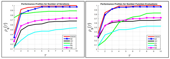
Figure 1.
Representation of the curve of the function for 6 methods with respect to Itr and FEs criteria.
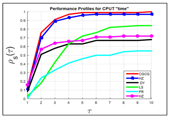
Figure 2.
Representation of the curve of function of six methods regarding CPU time criterion.
The results in Table 1 present the number of iterations (Itr) for all six CG parameters. It is clear that the CGCG algorithm (Algorithm 1) was capable of solving all the test problems (76 benchmark test problems).
Hence, the CGCG method satisfies the following condition (success standard): Itr and , for all test problems. The second-best performance was exhibited by the HZ method.
According to the graph on the left of Figure 1 with , the success rates of the six algorithms are ordered as follows: , , , , , and , for CGCG, HZ, DY, LS, FR, and HS, respectively.
The performance of the six algorithms examined via performance profiles is shown in Figure 1 and Figure 2. By utilizing the performance profile theory, we generated three performance levels, which are shown Figure 1 and Figure 2.
These two figures are based on the results listed in Table 1, Table 2 and Table 3 for the Itr, EFs, and CPU time for all 76 test problems, respectively.
It is clear from the two figures that the CGCG algorithm has the characteristics of efficiency, reliability, and effectiveness in solving the 76 test problems compared to the other five methods.
The performance of the six algorithms can be summarized by referencing Figure 1 and Figure 2, as follows. The performance of the six methods with respect to the Itr criterion is shown as follows.
At , the success rates of the 6 algorithms are arranged as follows: , , , , , and for the LS, CGCG, HZ, HS, FR, and DY methods, respectively, corresponding to the left graph in Figure 1.
At , the success rates of the six algorithms are ordered as follows: , , , , , and for the CGCG, HZ, LS, HS, DY, and FR, respectively, as shown in the left graph in Figure 1.
At , the success rates of the six algorithms are ordered as follows: , , , , and for the CGCG, HZ, LS, HS, DY, and FR, respectively, as shown in the left graph in Figure 1.
At , the success rates of the six algorithms are ordered as follows: , , , , , and for the CGCG, HZ, LS, HS, DY, and FR methods, respectively, shown in the left graph in Figure 1.
At , the success rates of the six algorithms are ordered as follows: , , , , , and for the CGCG, HZ, LS, HS, DY, and FR methods, respectively, as shown in the left graph of Figure 1.
At , the success rates of the six algorithms are ordered as follows: , , , , and for the CGCG, HZ, LS, HS, DY, and FR methods, respectively, as shown in the left graph in Figure 1.
At , the success rates of the six algorithms are ordered as follows: , , , , , and for the CGCG, HZ, LS, HS, DY, and FR methods, respectively, as shown in the left graph in Figure 1.
At , the success rates of the six algorithms are ordered as follows: , , , , , and for the CGCG, HZ, LS, HS, DY, and FR methods, respectively, as shown in the left graph in Figure 1.
At , the success rates of the six algorithms are ordered as follows: , , , , , and for the CGCG, HZ, LS, HS, DY, and FR methods, respectively, as shown in the left graph in Figure 1.
At , the success rates of the six algorithms are ordered as follows: , , , , , and for the CGCG, HZ, LS, HS, DY, and FR methods, respectively, as shown in the left graph in Figure 1.
The performance of the six methods with respect to the FEs criterion is shown as follows.
At , the success rates of the six algorithms are ordered as follows: , , , , , and , for the CGCG, HS, HZ, DY, LS, and FR, methods, respectively, as shown in the right graph of Figure 1.
At , the success rates of the six algorithms are ordered as follows: , , , , , and , for the CGCG, HZ, DY, HS, FR, and LS methods, respectively, in the right-hand graph in Figure 1.
At , the success rates of the six algorithms are ordered as follows: , , , , and , for the CGCG, HZ, HS, DY, FR and LS, for the right graph of Figure 1.
At , the success rates of the six algorithms are ordered as follows: , , , , and , for the CGCG, HZ, HS, DY, LS and FR for the right graph of Figure 1.
At , the success rates of the six algorithms are ordered as follows: , , , , and , for the CGCG, HZ, HS, LS, DY and FR for the right graph of Figure 1.
At , the success rates of the six algorithms are ordered as follows: , , , , and , for the CGCG, HZ, LS, HS, DY and FR for the right graph of Figure 1.
At , the success rates of the six algorithms are ordered as follows: , , , , and , for the CGCG, HZ, LS, HS, DY and FR for the right graph of Figure 1.
At , the success rates of the six algorithms are ordered as follows: , , , , and , for the CGCG, HZ, LS, HS, DY and FR for the right graph of Figure 1.
At , the success rates of the six algorithms are ordered as follows: , , , , and , for the CGCG, HZ, LS, HS, DY and FR for the right graph of Figure 1.
At , the success rates of the six algorithms are ordered as follows: , , , , , , for the CGCG, HZ, LS, HS, DY, and FR for the right graph of Figure 1.
In addition, for Figure 2 and at , the success rates of the six algorithms are ordered as follows , , , , and for the CGCG, HZ, DY, LS, FR, and HS methods, respectively.
In general, all the graphs show that the curve of the function is almost maximal for the CGCG method. Therefore, the comparison results indicate that the CGCG approach is competitive with, and in all cases superior to, the five other CG methods in terms of efficiency, reliability, and effectiveness with regard to solving the set of test problems.
4. Image Processing
This section constitutes the second part of our numerical experiments. This section aims to render the CGCG algorithm capable of dealing with image-processing problems.
Images are often corrupted by various sources (factors) that may be responsible for the introduction of an artifact in a photo.
Therefore, the number of degraded pixels in a photo corresponds to the amount of noise that has been introduced into the image.
The main sources of noise in a digital image are as follows: [71,72].
- Some environmental conditions may impact the efficiency of an imaging sensor during image acquisition.
- Noise may be introduced into an image through an inappropriate sensor temperature and low light levels.
- In addition, an image can deteriorated (corrupted) due to interference in the transmission channel.
- Similarly, the image may be deteriorated (corrupted) due to dust particles that may exist on the scanner screen.
Images are often deteriorated by batch fuzz due to noisy sensors or transmission channels that lead to the corruption of a number of pixels in the picture.
A batch fuzz is one of the numerous popular noise samples in which only a portion of the pixels is degraded, i.e., the information of the pixels is entirely lost.
Generally, different photos with several implementations require treatment using a fine noise funnel technique to obtain credible effects and thus restore the original picture.
To restore an original photo that has been deteriorated by batch noise, a two-phase scheme is used, in which the first phase entails determining the fuzz-affected pixels in the corrupted photo, which is executed using the adaptive median filter algorithm [73,74,75,76,77].
In the first stage, the adaptive median filter algorithm determines the noise in the corrupted image, as follows. The filter compares each pixel in the distorted image to the surrounding pixels. If one of the pixel values varies significantly from the majority of the surrounding pixels, the pixel is treated as noise. More details about the adaptive median filter algorithm and salt-and-pepper noise removal by median type are available in [73,74,75,76,78,79].
The second phase of the scheme involves restoring the original image by using any algorithm that solves optimization problems.
Chan et al. [73] have applied the two-phase scheme to restore a corrupted image.
Many authors have used these two phases to render CG algorithms cable of restoring images corrupted by impulse noise (see, for example [25,42,43]).
The two-phase scheme can be briefly described as follows.
By applying the first stage, we use the adaptive median filter to select the corrupted pixels [73].
In the second phase, assume that the corrupted photo, denoted by , has a size of by and , constituting the index group of the photo .
The set denotes the set of indices of the noise pixels detected from the first phase, and is the number of elements of ℵ.
Let be the set of the four closest neighbors of the pixel at pixel location , i.e., let , and be the observed pixel value (gray level) of the photo at pixel location .
Therefore, in the second stage, the noise from the corrupted pixels is removed by solving the following non-smooth problem:
where , , and is a potential edge-preserving function.
Some of these functions were defined in [73], as follows.
In this paper, we use the second branch of (51), employing different values of the , and is a column vector of length ordered lexicographically.
However, it is time consuming and costly to determine the minimizer point of a non-smooth problem (50) exactly.
The authors of [80] canceled the non-smooth term and presented the subsequent smooth unconstrained optimization problem:
Clearly, the greater the fuzz ratio, the greater the size of (52).
Cai et al. [80] revealed that degraded pictures may be repaired efficiently by utilizing the CG parameters to find the minimizer of Problem (52); however, in reality, the fuzz ratio is heightened or actually corresponds to .
Newly proposed algorithms of CG parameters for solving this problem (image restoration) can be found in [25,42,81].
Now, we concentrate on using the two-stage procedure to clear salt-and-pepper fuzz that represents a particular state of batch noise.
The adaptive median filter approach that is described by the authors of [76] will be used as the first stage to detect noisy pixels.
Therefore, the CGCG method is modified to obtain three CGCG algorithms, which are adapted to solve Problem (52); hence, this case represents the second stage.
The following iterative form is used to generate the candidate solutions of Problem (52).
where represents the step size computed by a line search method, and is the search direction, which is defined as follows.
where .
This combination allows for the acquisition of integrated algorithms that inherit the features of the parameters defined in Formulas (4), (9), (25), and (27).
Therefore, the two Formulas (53) and (54) can be run iteratively through one of the following cases.
Case 1: If , then the CGCG-SH algorithm is used.
Case 2: If , then the CGCG-HZ algorithm is used.
The selected size of the filter window for the adaptive median filter method has a key role in the phases uncovering the noisy pixels in the corrupted image.
Chan et al. [73] presented several volumes of the filter window (W) as noted by the fuzz level as follows:
When the noise level is less than , then the maximum of the window is . When the noise level is between and , ; if the noise level is between and , ; if the noise level is between and , ; if the noise level is between and , ; if the noise level is between and , ; and if the noise level is between and , .
In addition, the value of in Problem (52) may be significant for finding the minimizer of Problem (52). Cai et al. [80] set .
Accordingly, we suggest two diffident values of the filter window (W) and the parameter , as follows.
Procedure: A We set , and if the noise ratio is less than or equal to , then we set . Otherwise we set .
Consequently, by using Procedure: A and both Case 1 and Case 2, we design two algorithms for solving Problem (52). These tow algorithms are the CGCG-HS1 algorithm and CGCG-HZ algorithm; the research directions of the two algorithms are defined by
and
respectively.
Procedure: B If the noise ratio is equal to , we set ; if the noise ratio equals , we set ; if the noise ratio is equal to , we set ; and if the noise ratio is equal to , we set . Additionally, we set for any noise level.
According to Procedure: B, we used Formula (55) to solve all images problems; this algorithm is abbreviated as CGCG-HS2.
We assess the performance of these three incorporated algorithms in solving image restoration problems by utilizing the peak signal-to-noise ratio [82].
The peak signal-to-fuzz proportion (PSNR) is defined as follows:
where and are the pixel values of the fixed picture and the original one, respectively.
The examined pictures are Lena (), Hill (), Man (), and Boat ().
The stopping standard used is defined by the following conditions.
If one of the two conditions is met, or
The above procedures can be summarized as the following algorithms.
For further clarification of the working mechanism of the three proposed algorithms listed in Algorithms 2–4, the steps applied are shown in Figure 3.
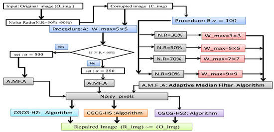
Figure 3.
Flowchart of the proposed algorithms CGCG-HS1, CGCG-HS2, and CGCG-HZ.
In addition, Figure 4 depicts a graphical abstract of the operational scheme of the three proposed algorithms with real examples.
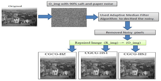
Figure 4.
A graphical abstract of the wormking mechanism of CGCG-HS1, CGCG-HS2, and CGCG-HZ.
5. Numerical Results
In this section, we use the same operating environment that is used in Section 3.
Therefore, three criteria are used in this section; these standards are the Itr CPU time (Tcpu) and the PSNR values for the restored images listed in Table 4.
Table 4.
Results regarding the performance of CGCG-HS1, CGCG-HS2, and CGCG-HZ Algorithms for repairing corrupted pictures.
In addition, the graphs of the original, noisy, and repaired pictures are shown in Figure 5, Figure 6, Figure 7 and Figure 8.
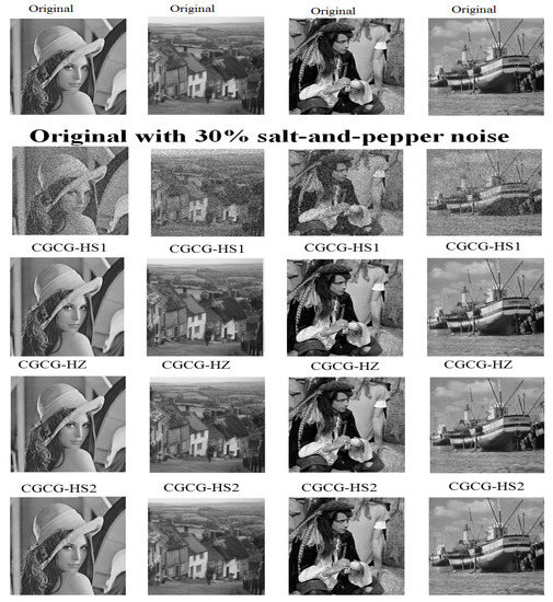
Figure 5.
Initial pictures (1st row), the noisy photos with 30% salt-and-pepper fuzz (2nd row), and the pictures repaired by CGCG-HS1 (3rd row), CGCG-HZ (4th row), and CGCG-HS2 (5th row).
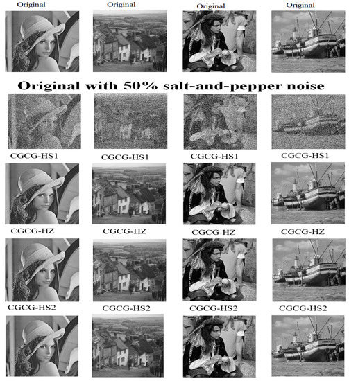
Figure 6.
Initial Photos (1st row), the noisy photos with 50% salt-and-peppernoise (2nd row), and the repaired images by CGCG-HS1 (3rd row), CGCG-HZ (4th row), and CGCG-HS2 (5th row).
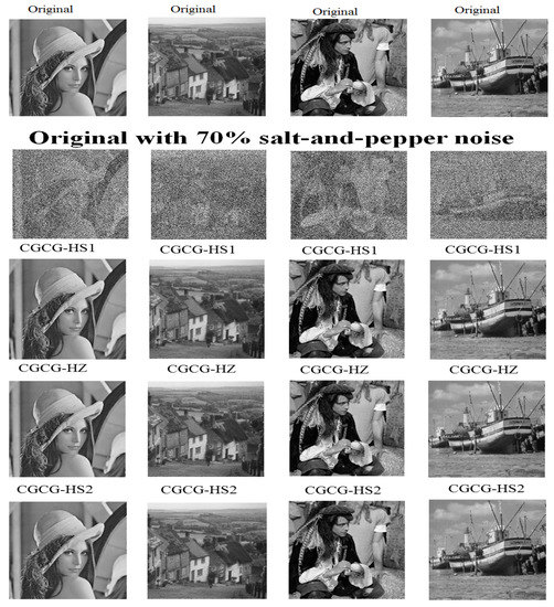
Figure 7.
Initial pictures (1st row), the noisy pictures with 70% salt-and-pepper noise (2nd row), and the repaired pictures by CGCG-HS1 (3rd row), CGCG-HZ (4th row), and CGCG-HS2 (fifth row).
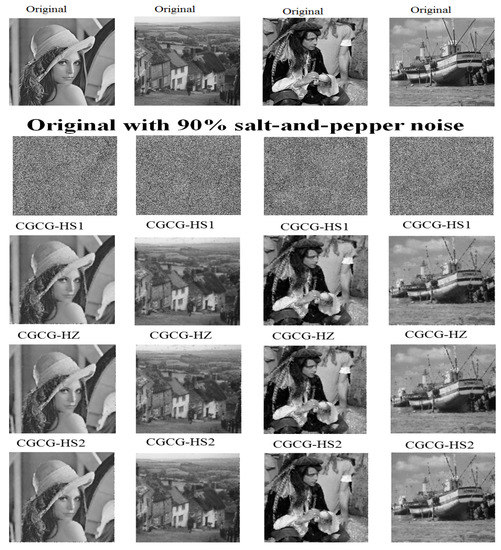
Figure 8.
Initial pictures (1st row), the noisy pictures with 90% salt-and-pepper noise (2nd row), and the repaired pictures by CGCG-HS1 (3rd row), CGCG-HZ (4th row), and CGCG-HS2 (5th row).
The noise levels of the salt-and-pepper noise are as follows: , , , and .
The fifth row of Table 4 offers the totals of the three standards, i.e., Itr, Tcpu, and PSNR, for the repaired pictures. These pictures were processed by three algorithms: CGCG-HS1, CGCG-HZ, and CGCG-HS2.
These three criteria show that the CGCG-HS1 algorithm has achieved the best results for the PSNR compared to the CGCG-HS2 and CGCG-HZ algorithms.
With respect to time (Tcpu) and the number of iterations (Itr), the CGCG-HZ algorithm is the best, as it restores all corrupted images of all noises levels within 441.33 s with 288 iterations versus 525.62 s and 324 iterations achieved by applying the CGCG-HS1 algorithm and 525.738 s and 332 iterations achieved using CGCG-HS2 method. However, the CGCG-HS1 algorithm is the best for PSNR, as it its time span is 479.58 against 479.02 and 479.35 for CGCG-HZ and CGCG-HS2, respectively.
In general, the performance of the CGCG-HS1 and CGCG-HZ algorithms is better than the performance of the CGCG-HS2 algorithm. This means that the value of the parameter plays a key role in minimizing the objective function in (52); additionally, the size of the filter window in the adaptive median filter method is very significant when scanning a deteriorated image. The outstanding clarity of the restored images proves the new family of modified hybrid CG methods can be used to solve many problems in different applications.
6. Conclusions and Future Work
A novel four-term CG parameter has been designed and tested in this study. The newly proposed algorithm is abbreviated as CGCG, which stands for “Convex Group Conjugated Gradient”.
The CGCG algorithm solved an unconstrained optimization problem.
The convergence analysis proof of the CGCG approach has been shown. Through solving a set 76 benchmark test problems using the six algorithms, the numerical results indicate that the CGCG algorithm outperforms the five classical CG algorithms. The CGCG algorithm has been adapted into a new family of modified CG methods used to deal with image restoration problems. The median filter method was first applied to detect the noise in a corrupted image. According to the noise level in the corrupted image, we changed the size of the filter window to improve the performance of this proposed family of CG methods. The salt-and-pepper technique was used to corrupt an image as a test problem, where levels of noise are 30–90%. Therefore, four well-known images (test problems) were corrupted with salt-and-pepper noise (at levels from 30 to 90%) to examine the performance of the new family of modified hybrid CG methods.
The superior clarity of the restored images indicates that the new family of modified hybrid CG methods has efficiency, reliability, and effectiveness in dealing with image restoration problems.
Therefore, this new family of modified hybrid CG methods can be adapted to deal with other problems in different applications. In future research, it will be valuable to combine the CGCG method with a meta-heuristic technique in order to possess the features of both techniques. Through this hybridization, we will obtain a hybrid CG meta-heuristic algorithm for dealing with global optimization problems, including unconstrained, constrained, and multi-objective problems.
It is also useful to develop the CGCG approach to deal with a nonlinear system of monotone equations.
Furthermore, the CGCG approach could be modified to deal with the symmetric system of nonlinear equations, image restoration, and deep neural networks used for trains.
7. List of Test Problem
These test problems were taken from [65,66].
COSINE function (CUTE): Pr = 1–3
DIXMAAN function (CUTE): Pr = 4–26
where .
| A | 1 | 0 | 0.125 | 0.125 | 0 | 0 | 0 | 0 |
| B | 1 | 0.0625 | 0.0625 | 0.0625 | 0 | 0 | 0 | 1 |
| C | 1 | 0.125 | 0.125 | 0.125 | 0 | 0 | 0 | 0 |
| D | 1 | 0.26 | 0.26 | 0.26 | 0 | 0 | 0 | 0 |
| E | 1 | 0 | 0.125 | 0.125 | 1 | 0 | 0 | 1 |
| F | 1 | 0.0625 | 0.0625 | 0.0625 | 1 | 0 | 0 | 1 |
| G | 1 | 0.125 | 0.125 | 0.125 | 1 | 0 | 0 | 1 |
| H | 1 | 0.26 | 0.26 | 0.26 | 1 | 0 | 0 | 1 |
| I | 1 | 0 | 0.125 | 0.125 | 2 | 0 | 0 | 2 |
| J | 1 | 0.0625 | 0.0625 | 0.0625 | 2 | 0 | 0 | 2 |
| K | 1 | 0.125 | 0.125 | 0.125 | 2 | 0 | 0 | 2 |
| L | 1 | 0.26 | 0.26 | 0.26 | 2 | 0 | 0 | 2 |
DIXON3DQ function (CUTE): Pr = 27
DQDRTIC function (CUTE): Pr = 28–31
EDENSCH function (CUTE): Pr = 32–34
EG2 function (CUTE): Pr = 35
FLETCHCR function (CUTE): Pr = 36–38
HIMMELBG function (CUTE): Pr = 39–40
LIARWHD function (CUTE): Pr = 41–42
Extended Penalty function: Pr = 43–44
QUARTC function (CUTE): Pr = 45–47
TRIDIA function (CUTE): Pr = 48–49
Extended Wood function: Pr = 50
.
BDEXP function (CUTE): Pr = 51–53
BIGGSB 1 function (CUTE): Pr = 54
SINE function: Pr = 55–57
FLETCBV3 function (CUTE): Pr = 58
where , , and .
NONSCOMP function (CUTE): Pr = 59–60
POWER function (CUTE): Pr = 61
Raydan 1 function: Pr = 62–63
Raydan 2 function: Pr = 64–66
Diagonal 1 function: Pr = 67–68
Diagonal 2 function: Pr = 69–70
Diagonal 3 function: Pr = 71–72
Extended Rosenbrock function: Pr = 73–74
TRIDIA function (CUTE): Pr = 75–76
Author Contributions
Conceptualization, E.A.; methodology, E.A. and S.M.; software, E.A. and S.M.; validation, E.A.; formal analysis, E.A.; investigation, E.A.; Funding acquisition, E.A.; data curation, E.A.; writing—original draft preparation, E.A. and S.M.; writing—review and editing E.A. and S.M.; visualization, E.A. and S.M.; supervision, E.A. and S.M. All authors have read and agreed to the published version of the manuscript.
Funding
This research was funded by the Deanship of Scientific Research at Najran University (grant number NU/DRP/SERC/12/3).
Data Availability Statement
Not applicable.
Acknowledgments
The authors are thankful to the Deanship of Scientific Research at Najran University for funding this work under the Research Priorities and Najran Research funding program grant number (NU/DRP/SERC/12/3).
Conflicts of Interest
The authors declare no conflict of interest.
References
- Hager, W.W.; Zhang, H. Algorithm 851: Cg_descent, a conjugate gradient method with guaranteed descent. ACM Trans. Math. Softw. 2006, 32, 113–137. [Google Scholar] [CrossRef]
- Andrei, N. Conjugate Gradient Methods; Springer International Publishing: Cham, Switzerland, 2022; pp. 169–260. ISBN 978-3-031-08720-2. [Google Scholar]
- Brown, P.N.; Saad, Y. Convergence theory of nonlinear newton—Krylov algorithms. SIAM J. Optim. 1994, 4, 297–330. [Google Scholar] [CrossRef]
- Li, D.-H.; Fukushima, M. A modified bfgs method and its global convergence in nonconvex minimization. J. Comput. Appl. Math. 2001, 129, 15–35. [Google Scholar] [CrossRef]
- Ali, E.; Mahdi, S. Adaptive hybrid mixed two-point step size gradient algorithm for solving non-linear systems. Mathematics 2023, 11, 2102. [Google Scholar] [CrossRef]
- Alnowibet, K.A.; Mahdi, S.; El-Alem, M.; Abdelawwad, M.; Mohamed, A.W. Guided hybrid modified simulated annealing algorithm for solving constrained global optimization problems. Mathematics 2022, 10, 1312. [Google Scholar] [CrossRef]
- L-Alem, M.E.; Aboutahoun, A.; Mahdi, S. Hybrid gradient simulated annealing algorithm for finding the global optimal of a nonlinear unconstrained optimization problem. Soft Comput. 2020, 25, 2325–2350. [Google Scholar] [CrossRef]
- Fletcher, R.; Reeves, C.M. Function minimization by conjugate gradients. Comput. J. 1964, 7, 149–154. [Google Scholar] [CrossRef]
- Hestenes, M.R.; Stiefel, E. Methods of conjugate gradients for solving. J. Res. Natl. Bur. Stand. 1952, 49, 409. [Google Scholar] [CrossRef]
- Liu, Y.; Storey, C. Efficient generalized conjugate gradient algorithms, part 1: Theory. J. Optim. Theory Appl. 1991, 69, 129–137. [Google Scholar] [CrossRef]
- Polak, E.; Ribiere, G. Note sur la convergence de méthodes de directions conjuguées. ESAIM Math. Model. Numer. Anal. Model. Math. Anal. Numer. 1969, 3, 35–43. [Google Scholar] [CrossRef]
- Argyros, I.K. Convergence and Applications of Newton-Type Iterations; Springer Science & Business Media: Berlin/Heidelberg, Germany, 2008. [Google Scholar]
- Birgin, E.G.; Krejić, N.; Martínez, J.M. Globally convergent inexact quasi-newton methods for solving nonlinear systems. Numer. Algorithms 2003, 32, 249–260. [Google Scholar] [CrossRef]
- Li, D.; Fukushima, M. A globally and superlinearly convergent gauss—Newton-based bfgs method for symmetric nonlinear equations. SIAM J. Numer. Anal. 1999, 37, 152–172. [Google Scholar] [CrossRef]
- Li, D.-H.; Fukushima, M. A derivative-free line search and global convergence of broyden-like method for nonlinear equations. Optim. Methods Softw. 2000, 13, 181–201. [Google Scholar] [CrossRef]
- Solodov, M.V.; Svaiter, B.F. A globally convergent inexact newton method for systems of monotone equations. In Reformulation: Nonsmooth, Piecewise Smooth, Semismooth and Smoothing Methods; Springer: Berlin/Heidelberg, Germany, 1998; pp. 355–369. [Google Scholar]
- Zhou, G.; Toh, K.-C. Superlinear convergence of a newton-type algorithm for monotone equations. J. Optim. Theory Appl. 2005, 125, 205–221. [Google Scholar] [CrossRef]
- Golub, G.H.; O’Leary, D.P. Some history of the conjugate gradient and lanczos algorithms: 1948–1976. SIAM Rev. 1989, 31, 50–102. [Google Scholar] [CrossRef]
- Hager, W.W.; Zhang, H. A survey of nonlinear conjugate gradient methods. Pac. J. Optim. 2006, 2, 35–58. [Google Scholar]
- Abubakar, A.B.; Malik, M.; Kumam, P.; Mohammad, H.; Sun, M.; Ibrahim, A.H.; Kiri, A.I. A liu-storey-type conjugate gradient method for unconstrained minimization problem with application in motion control. J. King Saud Univ.-Sci. 2022, 34, 101923. [Google Scholar] [CrossRef]
- Alnowibet, K.A.; Mahdi, S.; Alshamrani, A.M.; Sallam, K.M.; Mohamed, A.W. A family of hybrid stochastic conjugate gradient algorithms for local and global minimization problems. Mathematics 2022, 10, 3595. [Google Scholar] [CrossRef]
- Alshamrani, A.M.; Alrasheedi, A.F.; Alnowibet, K.A.; Mahdi, S.; Mohamed, A.W. A hybrid stochastic deterministic algorithm for solving unconstrained optimization problems. Mathematics 2022, 10, 3032. [Google Scholar] [CrossRef]
- Deng, S.; Wan, Z. A three-term conjugate gradient algorithm for large-scale unconstrained optimization problems. Appl. Numer. Math. 2015, 92, 70–81. [Google Scholar] [CrossRef]
- Jian, J.; Liu, P.; Jiang, X.; Zhang, C. Two classes of spectral conjugate gradient methods for unconstrained optimizations. J. Appl. Math. Comput. 2022, 68, 4435–4456. [Google Scholar] [CrossRef]
- Jiang, X.; Liao, W.; Yin, J.; Jian, J. A new family of hybrid three-term conjugate gradient methods with applications in image restoration. Numer. Algorithms 2022, 91, 161–191. [Google Scholar] [CrossRef]
- Abubakar, A.B.; Kumam, P. A descent dai-liao conjugate gradient method for nonlinear equations. Numer. Algorithms 2019, 81, 197–210. [Google Scholar] [CrossRef]
- Abubakar, A.B.; Kumam, P.; Awwal, A.M.; Thounthong, P. A modified self-adaptive conjugate gradient method for solving convex constrained monotone nonlinear equations for signal recovery problems. Mathematics 2019, 7, 693. [Google Scholar] [CrossRef]
- Abubakar, A.B.; Kumam, P.; Mohammad, H.; Awwal, A.M. An efficient conjugate gradient method for convex constrained monotone nonlinear equations with applications. Mathematics 2019, 7, 767. [Google Scholar] [CrossRef]
- Aji, S.; Kumam, P.; Awwal, A.M.; Yahaya, M.M.; Sitthithakerngkiet, K. An efficient dy-type spectral conjugate gradient method for system of nonlinear monotone equations with application in signal recovery. Aims. Math. 2021, 6, 8078–8106. [Google Scholar] [CrossRef]
- Althobaiti, A.; Sabi’u, J.; Emadifar, H.; Junsawang, P.; Sahoo, S.K. A scaled dai-yuan projection-based conjugate gradient method for solving monotone equations with applications. Symmetry 2022, 14, 1401. [Google Scholar] [CrossRef]
- Ibrahim, A.H.; Kumam, P.; Abubakar, A.B.; Abubakar, J.; Muhammad, A.B. Least-square-based three-term conjugate gradient projection method for l 1-norm problems with application to compressed sensing. Mathematics 2020, 8, 602. [Google Scholar] [CrossRef]
- Sabi’u, J.; Muangchoo, K.; Shah, A.; Abubakar, A.B.; Aremu, K.O. An inexact optimal hybrid conjugate gradient method for solving symmetric nonlinear equations. Symmetry 2021, 13, 1829. [Google Scholar] [CrossRef]
- Su, Z.; Li, M. A derivative-free liu—Storey method for solving large-scale nonlinear systems of equations. Math. Probl. Eng. 2020, 2020, 6854501. [Google Scholar] [CrossRef]
- Sulaiman, I.M.; Awwal, A.M.; Malik, M.; Pakkaranang, N.; Panyanak, B. A derivative-free mzprp projection method for convex constrained nonlinear equations and its application in compressive sensing. Mathematics 2022, 10, 2884. [Google Scholar] [CrossRef]
- Yuan, G.; Li, T.; Hu, W. A conjugate gradient algorithm for large-scale nonlinear equations and image restoration problems. Appl. Numer. Math. 2020, 147, 129–141. [Google Scholar] [CrossRef]
- Abubakar, A.B.; Muangchoo, K.; Ibrahim, A.H.; Muhammad, A.B.; Jolaoso, L.O.; Aremu, K.O. A new three-term hestenes-stiefel type method for nonlinear monotone operator equations and image restoration. IEEE Access 2021, 9, 18262–18277. [Google Scholar] [CrossRef]
- Aji, S.; Kumam, P.; Siricharoen, P.; Abubakar, A.B.; Yahaya, M.M. A modified conjugate descent projection method for monotone nonlinear equations and image restoration. IEEE Access 2020, 8, 158656–158665. [Google Scholar] [CrossRef]
- Chen, X.; Zhou, W. Smoothing nonlinear conjugate gradient method for image restoration using nonsmooth nonconvex minimization. SIAM J. Imaging Sci. 2010, 3, 765–790. [Google Scholar] [CrossRef]
- Ibrahim, A.H.; Kumam, P.; Abubakar, A.B.; Yusuf, U.B.; Yimer, S.E.; Aremu, K.O. An efficient gradient-free projection algorithm for constrained nonlinear equations and image restoration. Aims. Math. 2020, 6, 235. [Google Scholar] [CrossRef]
- Ibrahim, A.H.; Kumam, P.; Kumam, W. A family of derivative-free conjugate gradient methods for constrained nonlinear equations and image restoration. IEEE Access 2020, 8, 162714–162729. [Google Scholar] [CrossRef]
- Liu, Y.; Zhu, Z.; Zhang, B. Two sufficient descent three-term conjugate gradient methods for unconstrained optimization problems with applications in compressive sensing. J. Appl. Math. Comput. 2022, 68, 1787–1816. [Google Scholar] [CrossRef]
- Ma, G.; Lin, H.; Jin, W.; Han, D. Two modified conjugate gradient methods for unconstrained optimization with applications in image restoration problems. J. Appl. Math. Comput. 2022, 68, 4733–4758. [Google Scholar] [CrossRef]
- Malik, M.; Sulaiman, I.M.; Abubakar, A.B.; Ardaneswari, G.; Sukono. A new family of hybrid three-term conjugate gradient method for unconstrained optimization with application to image restoration and portfolio selection. AIMS Math. 2023, 8, 1–28. [Google Scholar] [CrossRef]
- Iiduka, H.; Kobayashi, Y. Training deep neural networks using conjugate gradient-like methods. Electronics 2020, 9, 1809. [Google Scholar] [CrossRef]
- Peng, C.-C.; Magoulas, G.D. Advanced adaptive nonmonotone conjugate gradient training algorithm for recurrent neural networks. Int. J. Artif. Intell. Tools 2008, 17, 963–984. [Google Scholar] [CrossRef]
- Sabir, Z.; Guirao, J.L. A soft computing scaled conjugate gradient procedure for the fractional order majnun and layla romantic story. Mathematics 2023, 11, 835. [Google Scholar] [CrossRef]
- Sabir, Z.; Said, S.B.; Guirao, J.L. A radial basis scale conjugate gradient deep neural network for the monkeypox transmission system. Mathematics 2023, 11, 975. [Google Scholar] [CrossRef]
- Xue, W.; Wan, P.; Li, Q.; Zhong, P.; Yu, G.; Tao, T. An online conjugate gradient algorithm for large-scale data analysis in machine learning. AIMS Math. 2021, 6, 1515–1537. [Google Scholar] [CrossRef]
- Polyak, B.T. The conjugate gradient method in extremal problems. USSR Comput. Math. Math. Phys. 1969, 9, 94–112. [Google Scholar] [CrossRef]
- Dai, Y.-H.; Yuan, Y. A nonlinear conjugate gradient method with a strong global convergence property. SIAM J. Optim. 1999, 10, 177–182. [Google Scholar] [CrossRef]
- Masmali, I.A.; Salleh, Z.; Alhawarat, A. A decent three term conjugate gradient method with global convergence properties for large scale unconstrained optimization problems. AIMS Math. 2021, 6, 10742–10764. [Google Scholar] [CrossRef]
- Yuan, G.; Jian, A.; Zhang, M.; Yu, J. A modified hz conjugate gradient algorithm without gradient lipschitz continuous condition for non convex functions. J. Appl. Math. Comput. 2022, 68, 4691–4721. [Google Scholar] [CrossRef]
- Mtagulwa, P.; Kaelo, P. An efficient modified prp-fr hybrid conjugate gradient method for solving unconstrained optimization problems. Appl. Numer. Math. 2019, 145, 111–120. [Google Scholar] [CrossRef]
- Hager, W.W.; Zhang, H. A new conjugate gradient method with guaranteed descent and an efficient line search. SIAM J. Optim. 2005, 16, 170–192. [Google Scholar] [CrossRef]
- Huo, J.; Yang, J.; Wang, G.; Yao, S. A class of three-dimensional subspace conjugate gradient algorithms for unconstrained optimization. Symmetry 2022, 14, 80. [Google Scholar] [CrossRef]
- Tian, Q.; Wang, X.; Pang, L.; Zhang, M.; Meng, F. A new hybrid three-term conjugate gradient algorithm for large-scale unconstrained problems. Mathematics 2021, 9, 1353. [Google Scholar] [CrossRef]
- Jian, J.; Yang, L.; Jiang, X.; Liu, P.; Liu, M. A spectral conjugate gradient method with descent property. Mathematics 2020, 8, 280. [Google Scholar] [CrossRef]
- Yunus, R.B.; Kamfa, K.; Mohammed, S.I.; Mamat, M. A novel three term conjugate gradient method for unconstrained optimization via shifted variable metric approach with application. In Intelligent Systems Modeling and Simulation II; Springer: Berlin/Heidelberg, Germany, 2022; pp. 581–596. [Google Scholar]
- Alhawarat, A.; Salleh, Z.; Masmali, I.A. A convex combination between two different search directions of conjugate gradient method and application in image restoration. Math. Probl. Eng. 2021, 2021, 9941757. [Google Scholar] [CrossRef]
- Zoutendijk, G. Nonlinear programming, computational methods. In Integer and Nonlinear Programming; North-Holland Publishing: Amsterdam, The Netherlands, 1970; pp. 37–86. [Google Scholar]
- Wolfe, P. Convergence conditions for ascent methods. SIAM Rev. 1969, 11, 226–235. [Google Scholar] [CrossRef]
- Wolfe, P. Convergence conditions for ascent methods. ii: Some corrections. SIAM Rev. 1971, 13, 185–188. [Google Scholar] [CrossRef]
- Cantrell, J.W. Relation between the memory gradient method and the fletcher-reeves method. J. Optim. Theory Appl. 1969, 4, 67–71. [Google Scholar] [CrossRef]
- Han, J.; Liu, G.; Yin, H. Convergence of perry and shanno’s memoryless quasi-newton method for nonconvex optimization problems. OR Trans. 1997, 1, 22–28. [Google Scholar]
- Andrei, N. An unconstrained optimization test functions collection. Adv. Model. Optim. 2008, 10, 147–161. [Google Scholar]
- Moré, J.J.; Garbow, B.S.; Hillstrom, K.E. Testing unconstrained optimization software. Acm Trans. Math. Softw. 1981, 7, 17–41. [Google Scholar] [CrossRef]
- Dolan, E.D.; Moré, J.J. Benchmarking optimization software with performance profiles. Math. Program. 2002, 91, 201–213. [Google Scholar] [CrossRef]
- Ali, M.M.; Khompatraporn, C.; Zabinsky, Z.B. A numerical evaluation of several stochastic algorithms on selected continuous global optimization test problems. J. Glob. Optim. 2005, 31, 635–672. [Google Scholar] [CrossRef]
- Barbosa, H.J.; Bernardino, H.S.; Barreto, A.M. Using performance profiles to analyze the results of the 2006 cec constrained optimization competition. In IEEE Congress on Evolutionary Computation; IEEE: Piscataway, NJ, USA, 2010; pp. 1–8. [Google Scholar]
- Vaz, A.I.F.; Vicente, L.N. A particle swarm pattern search method for bound constrained global optimization. J. Glob. Optim. 2007, 39, 197–219. [Google Scholar] [CrossRef]
- Mythili, C.; Kavitha, V.; Kavitha, D.V. Efficient technique for color image noise reduction. Res. Bull. Jordan Acm 2011, 2, 41–44. [Google Scholar]
- Verma, R.; Ali, J. A comparative study of various types of image noise and efficient noise removal techniques. Int. J. Adv. Res. Comput. Sci. Softw. Eng. 2013, 3, 617–622. [Google Scholar]
- Chan, R.H.; Ho, C.-W.; Nikolova, M. Salt-and-pepper noise removal by median-type noise detectors and detail-preserving regularization. IEEE Trans. Image Process. 2005, 141, 479–1485. [Google Scholar] [CrossRef]
- Chen, T.; Wu, H.R. Adaptive impulse detection using center-weighted median filters. IEEE Signal Process. Lett. 2001, 8, 1–3. [Google Scholar] [CrossRef]
- Gao, Z. An adaptive median filtering of salt and pepper noise based on local pixel distribution. In Proceedings of the 2018 International Conference on Transportation & Logistics, Information & Communication, Smart City (TLICSC 2018), Chengdu, China, 30–31 October 2018; Atlantis Press: Amsterdam, The Netherlands, 2018; pp. 473–483. [Google Scholar]
- Hwang, H.; Haddad, R.A. Adaptive median filters: New algorithms and results. IEEE Trans. Image Process. 1995, 4, 499–502. [Google Scholar] [CrossRef]
- Win, N.; Kyaw, K.; Win, T.; Aung, P. Image noise reduction using linear and non-linear filtering technique. Int. J. Sci. Res. Publ. 2019, 9, 816–821. [Google Scholar]
- Shrestha, S. Image denoising using new adaptive based median filters. arXiv 2014, arXiv:1410.2175. [Google Scholar] [CrossRef]
- Soni, H.; Sankhe, D. Image restoration using adaptive median filtering. Image 2019, 6, 841–844. [Google Scholar]
- Cai, J.-F.; Chan, R.; Morini, B. Minimization of an edge-preserving regularization functional by conjugate gradient type methods. In Image Processing Based on Partial Differential Equations; Springer: Berlin/Heidelberg, Germany, 2007; pp. 109–122. [Google Scholar]
- Yu, G.; Huang, J.; Zhou, Y. A descent spectral conjugate gradient method for impulse noise removal. Appl. Math. Lett. 2010, 23, 555–560. [Google Scholar] [CrossRef]
- Shih, F.Y. Image Processing and Pattern Recognition: Fundamentals and Techniques; John Wiley & Sons: Hoboken, NJ, USA, 2010. [Google Scholar]


Disclaimer/Publisher’s Note: The statements, opinions and data contained in all publications are solely those of the individual author(s) and contributor(s) and not of MDPI and/or the editor(s). MDPI and/or the editor(s) disclaim responsibility for any injury to people or property resulting from any ideas, methods, instructions or products referred to in the content. |
© 2023 by the authors. Licensee MDPI, Basel, Switzerland. This article is an open access article distributed under the terms and conditions of the Creative Commons Attribution (CC BY) license (https://creativecommons.org/licenses/by/4.0/).