Fluxbrane Polynomials and Melvin-like Solutions for Simple Lie Algebras

Abstract

This review dealt with generalized Melvin solutions for simple finite-dimensional Lie algebras. Each solution appears in a model which includes a metric and n scalar fields coupled to n Abelian 2-forms with dilatonic coupling vectors determined by simple Lie algebra of rank n. The set of n moduli functions $H_s\left(z\right)$ comply with n non-linear (ordinary) differential equations (of second order) with certain boundary conditions set. Earlier, it was hypothesized that these moduli functions should be polynomials in z (so-called “fluxbrane” polynomials) depending upon certain parameters $p_s>0$, $s=1,\dots ,n$. Here, we presented explicit relations for the polynomials corresponding to Lie algebras of ranks $n=1,2,3,4,5$ and exceptional algebra $E_6$. Certain relations for the polynomials (e.g., symmetry and duality ones) were outlined. In a general case where polynomial conjecture holds, 2-form flux integrals are finite. The use of fluxbrane polynomials to dilatonic black hole solutions was also explored.

1. Introduction

In this review article, we dealt with a certain generalization of the Melvin solution [1], which was studied earlier in Ref. [2]. It occurs in the model which contains metric, n Abelian 2-forms $F^s=d{A}^s$ and l scalar fields ${\phi }^{\alpha }$ ($l\ge n$). This solution is governed by a certain non-degenerate matrix $\left(A_{sl}\right)$ (“quasi-Cartan” matrix), $s,l=1,\dots ,n$. It is a particular case of the so-called generalized fluxbrane solutions presented earlier in Ref. [3].

The original $4d$ Melvin’s solution, which describes the gravitational field of a magnetic flux tube, has numerous multidimensional analogs, supported by certain configurations of form fields. These analogs are usually referred to as fluxbranes. The fluxbrane solutions originally appear in superstring/brane models. For generalized Melvin and fluxbrane solutions, see [4,5,6,7,8,9,10,11,12,13,14,15,16,17,18,19,20,21,22,23,24,25,26] and references therein.

It is important to note that the solutions from Ref. [3] are governed by a set of moduli functions $H_s\left(z\right)>0$ defined on the interval $(0,+\infty )$. Here, $z={\rho }^2$ and $\rho$ is a radial variable. These functions obey a set of n non-linear ordinary differential equations of second order—so-called master equations, governed by the matrix $\left(A_{s{s}^{\prime }}\right)$ (in fact, they are equivalent to Toda-like equations). The moduli functions should also obey the boundary conditions: $H_s(+0)=1$, $s=1,\dots ,n$.

Here, we assume that the matrix $\left(A_{s{s}^{\prime }}\right)$ is just a Cartan matrix of a simple finite-dimensional Lie algebra $\mathcal{G}$ of rank n. (Obviously, $A_{ss}=2$ for all s). Due to “polynomial conjecture” from Ref. [3], the solutions to master equations with the boundary conditions imposed have a polynomial structure:

$$H_s\left(z\right)=1+\sum _{k=1}^{n_s}{P}_s^{\left(k\right)}{z}^k,$$

(1)

where $P_s^{\left(k\right)}$ are constants ($P_s^{\left(n_s\right)}\ne 0$) and

$$n_s=2\sum _{s^{\prime }=1}^n{A}^{s{s}^{\prime }}.$$

(2)

Here, we denote $\left(A^{s{s}^{\prime }}\right)={\left(A_{s{s}^{\prime }}\right)}^{-1}$. The parameters $n_s$ are integers, which are called components of a twice-dual Weyl vector in the basis of simple roots [27].

In Refs. [2,28], a program (in Maple) for the calculation of these (fluxbrane) polynomials for a classical series of Lie algebras ($A_n$, $B_n$, $C_n$, $D_n$) was presented.

The fluxbrane polynomials $H_s$ define special solutions to open Toda chain equations [29,30,31,32], corresponding to simple finite-dimensional Lie algebra $\mathcal{G}$,

$$\frac{d^2{y}^s}{d{u}^2}=-4P_{s}exp\left(\sum _{l=1}^n{A}_{sl}{y}^l\right),$$

(3)

where

$$H_s=exp(-y^s\left(u\right)-n_{s}u),$$

(4)

$P_s>0$, $s=1,\dots ,n$, and $z=e^{-2u}$. These special solutions obey

$$y^s\left(u\right)=-n_{s}u+o\left(1\right),$$

(5)

as $u\to +\infty$.

In Section 2, we describe the generalized Melvin solution related to a simple finite-dimensional Lie algebra $\mathcal{G}$ [2]. In Section 3 and in Appendix A and Appendix B, we present fluxbrane polynomials for Lie algebras of ranks $n=1,2,3,4,5$ and also for $E_6$. Here, we also outline the so-called symmetry and duality identities for these polynomials and consider certain relations between them. In Section 4, we present calculations of 2-form flux integrals ${\mathsf{\Phi }}^s={\int }_{M_{*}}{F}^s$ over a certain $2d$ submanifold $M_{*}$. It is amazing that these integrals (fluxes) are finite for all parameters of fluxbrane polynomials. In Section 5, we outline possible applications of fluxbrane polynomials to dilatonic black hole solutions.

It should be noted that definitions of fluxbrane polynomials can be easily extended to (finite dimensional) semisimple Lie algebras.

2. The Solutions

We consider a model governed by the action

$$S=\int d^{D}x\sqrt{\left|g\right|}\left\{R\left[g\right]-h_{\alpha \beta }{g}^{MN}{\partial }_M{\phi }^{\alpha }{\partial }_N{\phi }^{\beta }-\frac{1}{2}\sum _{s=1}^{n}exp\left[2{\lambda }_s\left(\phi \right)\right]{\left(F^s\right)}^2\right\},$$

(6)

where $g=g_{MN}\left(x\right)d{x}^M\otimes d{x}^N$ is a metric, $\phi =\left({\phi }^{\alpha }\right)\in {\mathbb{R}}^l$ is a set of scalar fields, and $\left(h_{\alpha \beta }\right)$ is a constant symmetric non-degenerate $l\times l$ matrix $(l\in \mathbb{N})$, $F^s=d{A}^s=\frac{1}{2}{F}_{MN}^{s}d{x}^M\wedge d{x}^N$ is a 2-form, ${\lambda }_s$ is a 1-form on ${\mathbb{R}}^l$: ${\lambda }_s\left(\phi \right)={\lambda }_{s\alpha }{\phi }^{\alpha }$, $s=1,\dots ,n$; $\alpha =1,\&,l$. Here, $\left({\lambda }_{s\alpha }\right)$, $s=1,\dots ,n$, are dilatonic coupling vectors. In (6) we denote $\left|g\right|=|det(g_{MN}\left)\right|$, ${\left(F^s\right)}^2=F_{M_1{M}_2}^s{F}_{N_1{N}_2}^s{g}^{M_1{N}_1}{g}^{M_2{N}_2}$, $s=1,\dots ,n$.

Here, we deal with a family of exact solutions to field equations which correspond to the action (6) and depend on one variable $\rho$. These solutions are defined on the manifold,

$$M=(0,+\infty )\times M_1\times M_2,$$

(7)

where $M_1$ is a one-dimensional manifold (say $S^1$ or $\mathbb{R}$) and $M_2$ is a ($D-2$)-dimensional Ricci-flat manifold. The solution (from the family under consideration) reads [2]

$$\begin{array}{c}\hfill g=\left(\prod _{s=1}^n{H}_s^{2h_s/(D-2)}\right)\left\{wd\rho \otimes d\rho +\left(\prod _{s=1}^n{H}_s^{-2h_s}\right){\rho }^{2}d\varphi \otimes d\varphi +g^2\right\},\end{array}$$

(8)

$$\begin{array}{c}\hfill exp\left({\phi }^{\alpha }\right)=\prod _{s=1}^n{H}_s^{h_s{\lambda }_s^{\alpha }},\end{array}$$

(9)

$$\begin{array}{c}\hfill F^s=q_s\left(\prod _{l=1}^n{H}_l^{-A_{sl}}\right)\rho d\rho \wedge d\varphi ,\end{array}$$

(10)

$s=1,\dots ,n$; $\alpha =1,\dots ,l$, where $w=\pm 1$, $g^1=d\varphi \otimes d\varphi$ is a metric on $M_1$ and $g^2$ is a Ricci-flat metric on $M_2$. Here, $q_s\ne 0$ are integration constants ($q_s=-Q_s$ in notations of Ref. [2]), $s=1,\dots ,n$.

The moduli functions $H_s\left(z\right)>0$, $z={\rho }^2$ obey the master equations,

$$\frac{d}{dz}\left(\frac{z}{H_s}\frac{d}{dz}{H}_s\right)=P_s\prod _{l=1}^n{H}_l^{-A_{sl}},$$

(11)

with the following boundary conditions:

$$H_s(+0)=1,$$

(12)

where

$$P_s=\frac{1}{4}{K}_s{q}_s^2,$$

(13)

$s=1,\cdots ,n$. For $w=+1$, the boundary conditions (12) are necessary to avoid a conic singularity (for our metric (8)) in the limit $\rho =+0$.

The parameters $h_s$ obey the relations,

$$h_s=K_s^{-1},K_s=B_{ss}>0,$$

(14)

where

$$B_{s{s}^{\prime }}\equiv 1+\frac{1}{2-D}+{\lambda }_{s\alpha }{\lambda }_{s^{\prime }\beta }{h}^{\alpha \beta },$$

(15)

$s,s^{\prime }=1,\dots ,n$, with $\left(h^{\alpha \beta }\right)={\left(h_{\alpha \beta }\right)}^{-1}$. In the relations above we denote ${\lambda }_s^{\alpha }=h^{\alpha \beta }{\lambda }_{s\beta }$ and

$$\left(A_{s{s}^{\prime }}\right)=\left(2B_{s{s}^{\prime }}/B_{s^{\prime }{s}^{\prime }}\right).$$

(16)

This is the so-called quasi-Cartan matrix.

The constants $B_{s{s}^{\prime }}$ and $K_s=B_{ss}$ are related to scalar products of so-called “brane vectors” $U^s$, belonging to a certain linear space (in our case it has dimension $l+2$). We have $B_{s{s}^{\prime }}=(U^s,U^{s^{\prime }})$ and $K_s=(U^s,U^s)$, with certain scalar product $(.,.)$ defined in Refs. [33,34]. Such scalar products appear in various solutions with branes (black branes, fluxbranes, S-branes etc), e.g., in calculations of certain physical parameters (Hawking temperature, black hole/brane entropy, PPN parameters etc), see Ref. [34].

Product relation (16) defines generalized intersection rules for branes [33], while numbers $K_s$ are invariant under dimensional reductions with typical value $K_s=2$ for brane U-vectors which appear in numerous supergravity models, e.g., for $D=10,11$ [35].

It can be readily shown that if the matrix $\left(h_{\alpha \beta }\right)$ is of Euclidean signature, $l\ge n$, and $\left(A_{s{s}^{\prime }}\right)$ is a Cartan matrix of certain simple Lie algebra of rank n, then there exist co-vectors ${\lambda }_1,\dots ,{\lambda }_n$ obeying (16).

Our solution is nothing more than a special case of the fluxbrane (for $w=+1$, $M_1=S^1$) and S-brane ($w=-1$) solutions from Refs. [3,25], respectively.

If we put $w=+1$ and choose Ricci-flat metric $g^2$ of pseudo-Euclidean signature on manifold $M_2$ of dimension $d_2>2$, we obtain a higher dimensional generalization of the Melvin’s solution [1].

The Melvin’s solution does not contain scalar fields. It corresponds (in our notations) to $D=4$, $n=1$, $w=+1$, $l=0$, $M_1=S^1$ ($0<\varphi <2\pi$), $M_2={\mathbb{R}}^2$, $g^2=-dt\otimes dt+dx\otimes dx$, and Lie algebra $\mathcal{G}=A_1=\mathrm{sl}\left(2\right)$.

For the case of $w=-1$ and $g^2$ of Euclidean signature, one can obtain a cosmological solution with a horizon (as $\rho =+0$) if $M_1=\mathbb{R}$ ($-\infty <\varphi <+\infty$).

3. Examples of Solutions for Certain Lie Algebras

Here, we deal with the generalized Melvin-like solution for $n=l$, $w=+1$ and $M_1=S^1$, which corresponds to simple (finite dimensional) Lie algebra of certain rank n with the Cartan matrix $A=\left(A_{sl}\right)$.

We put here $h_{\alpha \beta }={\delta }_{\alpha \beta }$ and denote $\left({\lambda }_{s\alpha }\right)=\left({\lambda }_s^{\alpha }\right)={\overrightarrow{\lambda }}_s$, $s=1,\dots ,n$.

Due to (14)–(16) we get

$$K_s=\frac{D-3}{D-2}+{\overrightarrow{\lambda }}_s^2,$$

(17)

$h_s=K_s^{-1}$, and

$${\overrightarrow{\lambda }}_s{\overrightarrow{\lambda }}_l=\frac{1}{2}{K}_l{A}_{sl}-\frac{D-3}{D-2}\equiv G_{sl},$$

(18)

$s,l=1,\dots ,n$; (17) just follows from (18).

Remark 1. 

For large enough $K_s$ in (18) (or large enough ${\overrightarrow{\lambda }}_s^2$), there exist vectors ${\overrightarrow{\lambda }}_s$ obeying (18) (and hence (17)). Indeed, the matrix $G=\left(G_{sl}\right)$ is positive definite if $K_s>K_{*}$, where $K_{*}$ is some positive number. Hence, there exists a matrix Λ, such that ${\mathsf{\Lambda }}^T\mathsf{\Lambda }=G$. We put $\left({\Lambda }_{as}\right)=\left({\lambda }_s^a\right)$ and get a set of vectors obeying (18).

Here, as in [36], we use another parameter $p_s$ instead of $P_s$:

$$p_s=P_s/n_s,$$

(19)

$s=1,\dots ,n$. This is carried out to avoid big denominators for $P_s^{\left(k\right)}$ in relation (1).

Remark 2. 

The parameters $p_s$ give us the coefficients $P_s^{\left(1\right)}$ in (1):

$$P_s^{\left(1\right)}=P_s=p_s{n}_s,$$

(20)

$s=1,\dots ,n$. These relations can be readily obtained by putting $z=+0$ into master Equation (11) and using the boundary conditions (12). Moreover, for given Lie algebra one can deduce recurrent relations for higher coefficients $P_s^{(k+1)}$ in (1) as functions of $P_s^{\left(k\right)},\dots ,P_s^{\left(1\right)}=P_s$ and solve the chain of recurrent relations, justifying that $P_s^{(n_s+1)}=0$, for all $s=1,\dots ,n$.

We note also that, for a special choice of $p_s$ parameters: $p_s=p>0$, the polynomials have the following simple form [3]:

$$H_s\left(z\right)={(1+pz)}^{n_s},$$

(21)

$s=1,\dots ,n$. This relation may be considered a nice tool for the verification of general solutions for polynomials.

3.1. Rank-1 Case

${\mathit{A}}_{\mathbf{1}}$-case. We start with the simplest example, which occurs for the Lie algebra

$A_1=sl\left(2\right)$. We obtain [3]

$$H_1=1+p_{1}z.$$

(22)

Here, $n_1=1$.

In this case (due to (14)–(16)), we have

$$K_1=\frac{D-3}{D-2}+{\overrightarrow{\lambda }}_1^2,$$

(23)

$h_1=K_1^{-1}$.

Due to (22), we get the following asymptotical behavior:

$$H_1=H_1(z,p_1)\sim p_{1}z\equiv H_1^{as}(z,p_1),$$

(24)

as $z\to \infty$.

Relations (22) and (24) imply the following identity.

Duality Relation

Proposition 1. 

The fluxbrane polynomial corresponding to Lie algebra $A_1$ obeys for all $p_1\ne 0$ and $z\ne 0$ the identity

$$H_1(z,p_1)=H_1^{as}(z,p_1)H_1(z^{-1},p_1^{-1}).$$

(25)

3.2. Rank-2 Case

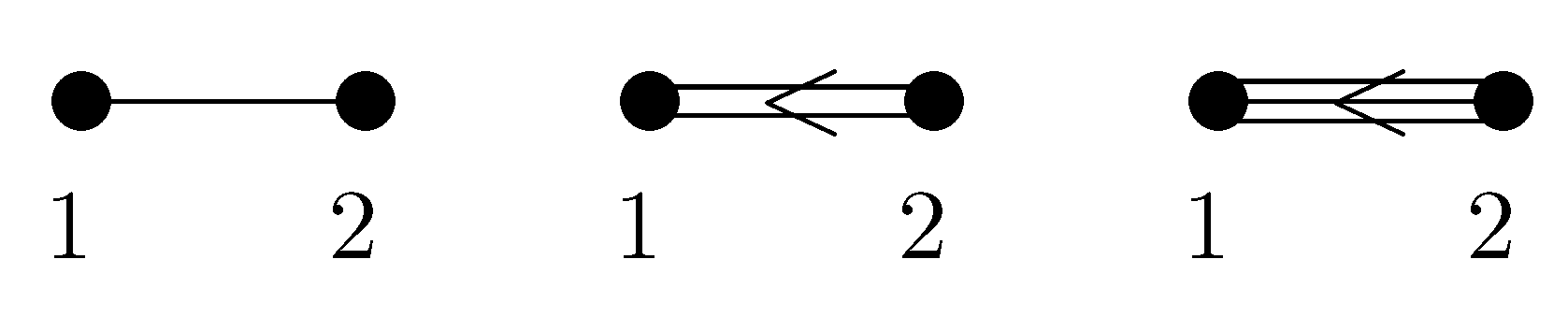
Now, we proceed with the solutions which correspond to simple Lie algebras $\mathcal{G}$ of rank 2, i.e., the matrix $A=\left(A_{sl}\right)$ is just a Cartan matrix,

$$\left(A_{s{s}^{\prime }}\right)=\left(\begin{array}{cc}2& -1\\ -k& 2\end{array}\right),$$

(26)

where $k=1,2,3$ for $\mathcal{G}=A_2,C_2\cong B_2,G_2$, respectively [37].

The matrix A is described graphically by the Dynkin diagrams presented in Figure 1 (for any of these three Lie algebras).

Figure 1. The Dynkin diagrams for the Lie algebras $A_2$, $C_2$, $G_2$, respectively.

It follows from (14)–(16) that

$$\frac{h_1}{h_2}=\frac{K_2}{K_1}=\frac{A_{21}}{A_{12}}=k,$$

(27)

where $k=1,2,3$ for $\mathcal{G}=A_2,C_2,G_2$, respectively.

3.2.1. Polynomials

${\mathit{A}}_{\mathbf{2}}$-case. For the Lie algebra $A_2=sl\left(3\right)$, we have [3,25,36]

$$\begin{array}{c}\hfill H_1=1+2p_{1}z+p_1{p}_2{z}^2,\end{array}$$

(28)

$$\begin{array}{c}\hfill H_2=1+2p_{2}z+p_1{p}_2{z}^2.\end{array}$$

(29)

${\mathit{C}}_{\mathbf{2}}$-case. In the case of Lie algebra $C_2=so\left(5\right)$, we get the following polynomials [25,36]:

$$\begin{array}{c}\hfill H_1=1+3p_{1}z+3p_1{p}_2{z}^2+p_1^2{p}_2{z}^3,\end{array}$$

(30)

$$\begin{array}{c}\hfill H_2=1+4p_{2}z+6p_1{p}_2{z}^2+4p_1^2{p}_2{z}^3+p_1^2{p}_2^2{z}^4.\end{array}$$

(31)

${\mathit{G}}_{\mathbf{2}}$-case. For the Lie algebra $G_2$, the fluxbrane polynomials read [25,36]:

$$\begin{array}{c}\hfill H_1=1+6p_{1}z+15p_1{p}_2{z}^2+20p_1^2{p}_2{z}^3+\\ \hfill 15p_1^3{p}_2{z}^4+6p_1^3{p}_2^2{z}^5+p_1^4{p}_2^2{z}^6,\end{array}$$

(32)

$$\begin{array}{c}\hfill H_2=1+10p_{2}z+45p_1{p}_2{z}^2+120p_1^2{p}_2{z}^3+p_1^2{p}_2(135p_1+75p_2)z^4\\ \hfill +252p_1^3{p}_2^2{z}^5+p_1^3{p}_2^2\left(75p_1+135p_2\right)z^6+120p_1^4{p}_2^3{z}^7\\ \hfill +45p_1^5{p}_2^3{z}^8+10p_1^6{p}_2^3{z}^9+p_1^6{p}_2^4{z}^{10}.\end{array}$$

(33)

Let us denote

$$H_s=H_s\left(z\right)=H_s(z,\left(p_i\right)),$$

(34)

$s=1,2$; where $\left(p_i\right)=(p_1,p_2)$.

We have the following asymptotical relations for polynomials:

$$H_s=H_s(z,\left(p_i\right))\sim \left(\prod _{l=1}^2{\left(p_l\right)}^{{\nu }^{sl}}\right)z^{n_s}\equiv H_s^{as}(z,\left(p_i\right)),$$

(35)

$s=1,2$, as $z\to \infty$.

Here, $\nu =\left({\nu }^{sl}\right)$ is the integer valued matrix,

$$\nu =\left(\begin{array}{cc}1& 1\\ 1& 1\end{array}\right),\left(\begin{array}{cc}2& 1\\ 2& 2\end{array}\right),\left(\begin{array}{cc}4& 2\\ 6& 4\end{array}\right),$$

(36)

for Lie algebras $A_2,C_2,G_2$, respectively.

For last two cases ($C_2$ and $G_2$), we have $\nu =2A^{-1}$ ($A^{-1}$ is inverse Cartan matrix). For the $A_2$-case, the matrix $\nu$ reads

$$\nu =A^{-1}(I+P),$$

(37)

where I is a $2\times 2$ identity matrix and

$$P=\left(\begin{array}{cc}0& 1\\ 1& 0\end{array}\right).$$

(38)

is a permutation matrix. It corresponds to the permutation $\sigma \in S_2$ ($S_2$ is symmetric group)

$$\sigma :(1,2)\mapsto (2,1),$$

(39)

by the following relation $P=\left(P_j^i\right)=\left({\delta }_{\sigma \left(j\right)}^i\right)$. Here, $\sigma$ is the generator of the group $S_2=\{\sigma ,id\}$—the group of symmetry of the Dynkin diagram (for $A_2$), which is isomorphic to the group $Z_2$.

Here, in all cases we get

$$\sum _{l=1}^2{\nu }^{sl}=n_s,$$

(40)

$s=1,2$.

Now, we denote ${\widehat{p}}_i=p_{\sigma \left(i\right)}$ for the $A_2$-case and ${\widehat{p}}_i=p_i$ for $C_2$ and $G_2$ cases, $i=1,2$. We call the ordered set $\left({\widehat{p}}_i\right)$ a dual one to the ordered set $\left(p_i\right)$. Using the relations for polynomials, we obtain the following identities (which can be readily verified just “by hands”).

3.2.2. Symmetry Relations

Proposition 2. 

The fluxbrane polynomials for $A_2$ obey for all $p_i$ and z the identities:

$$H_{\sigma \left(s\right)}(z,\left(p_i\right))=H_s(z,\left({\widehat{p}}_i\right)),$$

(41)

$s=1,2$.

3.2.3. Duality Relations

Proposition 3. 

The fluxbranes polynomials corresponding to Lie algebras $A_2$, $C_2$ and $G_2$ obey for all $p_i>0$ and $z>0$ the identities

$$H_s(z,\left(p_i\right))=H_s^{as}(z,\left(p_i\right))H_s(z^{-1},\left({\widehat{p}}_i^{-1}\right)),$$

(42)

$s=1,2$.

We call relations (42) duality ones.

3.3. Rank-3 Algebras

Now, we deal with polynomials which correspond to simple Lie algebras $\mathcal{G}$ of rank 3, when the matrix $A=\left(A_{sl}\right)$ coincides with one of the Cartan matrices,

$$\left(A_{s{s}^{\prime }}\right)=\left(\begin{array}{ccc}2& -1& 0\\ -1& 2& -1\\ 0& -1& 2\end{array}\right),\left(\begin{array}{ccc}2& -1& 0\\ -1& 2& -2\\ 0& -1& 2\end{array}\right),\left(\begin{array}{ccc}2& -1& 0\\ -1& 2& -1\\ 0& -2& 2\end{array}\right)$$

(43)

for $\mathcal{G}=A_3,B_3,C_3$, respectively [38].

Any of these matrices is described graphically by a Dynkin diagram pictured in Figure 2.

Figure 2. The Dynkin diagrams for the Lie algebras $A_3$, $B_3$, $C_3$, respectively.

It follows from (14), (16) that

$$\frac{h_s}{h_l}=\frac{K_l}{K_s}=\frac{B_{ll}}{B_{ss}}=\frac{B_{ls}}{B_{ss}}\frac{B_{ll}}{B_{sl}}=\frac{A_{ls}}{A_{sl}},$$

(44)

for any $s\ne l$ obeying $A_{sl},A_{ls}\ne 0$. This implies

$$K_1=K_2=K,K_3=K,\frac{1}{2}K,2K$$

(45)

or

$$h_1=h_2=h,h_3=h,2h,\frac{1}{2}h,$$

(46)

($h=K^{-1}$) for $\mathcal{G}=A_3,B_3,C_3$, respectively.

3.3.1. Polynomials

The set of moduli functions $(H_1\left(z\right),H_2\left(z\right),H_3\left(z\right))$, obeying Equations (11) and (12) with the matrix $A=\left(A_{sl}\right)$ from (43) are polynomials with powers $(n_1,n_2,n_3)=(3,4,3),(6,10,6),(5,8,9)$ for $\mathcal{G}=A_3,B_3,C_3$, respectively. We get the following polynomials [38].

${\mathit{A}}_{\mathbf{3}}$-case. For the Lie algebra $A_3\cong sl\left(4\right)$ we have [28,36]

$$\begin{array}{ccc}\hfill & & H_1=1+3p_{1}z+3p_1{p}_2{z}^2+p_1{p}_2{p}_3{z}^3,\hfill \end{array}$$

(47)

$$\begin{array}{ccc}\hfill & & H_2=1+4p_{2}z+(3p_1{p}_2+3p_2{p}_3)z^2+4p_1{p}_2{p}_3{z}^3+p_1{p}_2^2{p}_3{z}^4,\hfill \end{array}$$

(48)

$$\begin{array}{ccc}& & H_3=1+3p_{3}z+3p_2{p}_3{z}^2+p_1{p}_2{p}_3{z}^3.\hfill \end{array}$$

(49)

${\mathit{B}}_{\mathbf{3}}$-case. In the case of Lie algebra $B_3\cong so\left(7\right)$, the fluxbrane polynomials read [28]

$$H_1=1+6p_{1}z+15p_1{p}_2{z}^2+20p_1{p}_2{p}_3{z}^3+15p_1{p}_2{p}_3^2{z}^4+6p_1{p}_2^2{p}_3^2{z}^5+p_1^2{p}_2^2{p}_3^2{z}^6,$$

(50)

$$\begin{array}{cc}{H}_2\hfill & =1+10p_{2}z+\left(15p_1{p}_2+30p_2{p}_3\right)z^2+\left(80p_1{p}_2{p}_3+40p_2{p}_3^2\right)z^3\hfill \\ & +\left(50p_1{p}_2^2{p}_3+135p_1{p}_2{p}_3^2+25p_2^2{p}_3^2\right)z^4+252p_1{p}_2^2{p}_3^2{z}^5+\left(25p_1^2{p}_2^2{p}_3^2+135p_1{p}_2^3{p}_3^2+50p_1{p}_2^2{p}_3^3\right)z^6\hfill \\ & +\left(40p_1^2{p}_2^3{p}_3^2+80p_1{p}_2^3{p}_3^3\right)z^7+\left(30p_1^2{p}_2^3{p}_3^3+15p_1{p}_2^3{p}_3^4\right)z^8+10p_1^2{p}_2^3{p}_3^4{z}^9+p_1^2{p}_2^4{p}_3^4{z}^{10},\hfill \end{array}$$

(51)

$$\begin{array}{ccc}\hfill & & H_3=1+6p_{3}z+15p_2{p}_3{z}^2+\left(10p_1{p}_2{p}_3+10p_2{p}_3^2\right)z^3+15p_1{p}_2{p}_3^2{z}^4+6p_1{p}_2^2{p}_3^2{z}^5+p_1{p}_2^2{p}_3^3{z}^6.\hfill \end{array}$$

(52)

${\mathit{C}}_{\mathbf{3}}$-case. For the Lie algebra $C_3\cong sp\left(3\right)$, we obtain (with the use of MATHEMATICA) the following polynomials:

$$H_1=1+5p_{1}z+10p_1{p}_2{z}^2+10p_1{p}_2{p}_3{z}^3+5p_1{p}_2^2{p}_3{z}^4+p_1^2{p}_2^2{p}_3{z}^5,$$

(53)

$$\begin{array}{cc}{H}_2\hfill & =1+8p_{2}z+\left(10p_1{p}_2+18p_2{p}_3\right)z^2+\left(40p_1{p}_2{p}_3+16p_2^2{p}_3\right)z^3+70p_1{p}_2^2{p}_3{z}^4\hfill \\ & +\left(16p_1^2{p}_2^2{p}_3+40p_1{p}_2^3{p}_3\right)z^5+\left(18p_1^2{p}_2^3{p}_3+10p_1{p}_2^3{p}_3^2\right)z^6\hfill \\ & +8p_1^2{p}_2^3{p}_3^2{z}^7+p_1^2{p}_2^4{p}_3^2{z}^8,\hfill \end{array}$$

(54)

$$\begin{array}{cc}{H}_3\hfill & =1+9p_{3}z+36p_2{p}_3{z}^2+\left(20p_1{p}_2{p}_3+64p_2^2{p}_3\right)z^3+\left(90p_1{p}_2^2{p}_3+36p_2^2{p}_3^2\right)z^4\hfill \\ & +\left(36p_1^2{p}_2^2{p}_3+90p_1{p}_2^2{p}_3^2\right)z^5+\left(64p_1^2{p}_2^2{p}_3^2+20p_1{p}_2^3{p}_3^2\right)z^6\hfill \\ & +36p_1^2{p}_2^3{p}_3^2{z}^7+9p_1^2{p}_2^4{p}_3^2{z}^8+p_1^2{p}_2^4{p}_3^3{z}^9.\hfill \end{array}$$

(55)

We denote

$$H_s=H_s\left(z\right)=H_s(z,\left(p_i\right)),$$

(56)

where $\left(p_i\right)=(p_1,p_2,p_3)$.

Due to obtained relations for polynomials, we get the asymptotical behavior

$$H_s=H_s(z,\left(p_i\right))\sim \left(\prod _{l=1}^3{\left(p_l\right)}^{{\nu }^{sl}}\right)z^{n_s}\equiv H_s^{as}(z,\left(p_i\right)),$$

(57)

as $z\to \infty$.

Here, $\nu =\left({\nu }^{sl}\right)$ is the integer valued matrix

$$\nu =\left(\begin{array}{ccc}1& 1& 1\\ 1& 2& 1\\ 1& 1& 1\end{array}\right),\left(\begin{array}{ccc}2& 2& 2\\ 2& 4& 4\\ 1& 2& 3\end{array}\right),\left(\begin{array}{ccc}2& 2& 1\\ 2& 4& 2\\ 2& 4& 3\end{array}\right),$$

(58)

for Lie algebras $A_3,B_3,C_3$, respectively.

For Lie algebras $B_3$ and $C_3$ we have

$$\nu =2A^{-1},$$

(59)

where $A^{-1}$ is inverse Cartan matrix. For the $A_3$-case the matrix $\nu$ reads as follows:

$$\nu =A^{-1}(I+P),$$

(60)

where I is $3\times 3$ identity matrix and

$$P=\left(\begin{array}{ccc}0& 0& 1\\ 0& 1& 0\\ 1& 0& 0\end{array}\right)$$

(61)

is a permutation matrix, which corresponds to the permutation $\sigma \in S_3$ ($S_3$ is symmetric group)

$$\sigma :(1,2,3)\mapsto (3,2,1),$$

(62)

by the following formula $P=\left(P_j^i\right)=\left({\delta }_{\sigma \left(j\right)}^i\right)$. Here, $\sigma$ is the generator of the group $G=\{\sigma ,\mathrm{id}\}$—the group of symmetry of the Dynkin diagram (for $A_3$), which is isomorphic to the group ${\mathbb{Z}}_2$.

Here, in all three cases we have

$$\sum _{l=1}^3{\nu }^{sl}=n_s,$$

(63)

$s=1,2,3$.

Now, we introduce notations: ${\widehat{p}}_i=p_{\sigma \left(i\right)}$ for the $A_3$ and ${\widehat{p}}_i=p_i$ for $B_3$ and $C_3$ algebras, $i=1,2,3$. Using relations for rank-3 polynomials, we obtain (with a help of MATHEMATICA) the following identities.

3.3.2. Symmetry Relations

Proposition 4. 

The fluxbrane polynomials for $A_3$ algebra obey for all $p_i$ and z the identities:

$$H_{\sigma \left(s\right)}(z,\left(p_i\right))=H_s(z,\left({\widehat{p}}_i\right)),$$

(64)

$s=1,2,3$.

3.3.3. Duality Relations

Proposition 5. 

The fluxbranes polynomials corresponding to Lie algebras $A_3$, $B_3$ and $C_3$ obey for all $p_i>0$ and $z>0$ the identities

$$H_s(z,\left(p_i\right))=H_s^{as}(z,\left(p_i\right))H_s(z^{-1},\left({\widehat{p}}_i^{-1}\right)),$$

(65)

$s=1,2,3$.

3.4. Rank-4 Algebras

In this subsection, we deal with the solutions related to Lie algebras $\mathcal{G}$ of rank 4, i.e., the matrix $A=\left(A_{sl}\right)$ coincides with one of the Cartan matrices.

$$\begin{array}{cc}\hfill \left(A_{s{s}^{\prime }}\right)& =\left(\begin{array}{cccc}2& -1& 0& 0\\ -1& 2& -1& 0\\ 0& -1& 2& -1\\ 0& 0& -1& 2\end{array}\right),\left(\begin{array}{cccc}2& -1& 0& 0\\ -1& 2& -1& 0\\ 0& -1& 2& -2\\ 0& 0& -1& 2\end{array}\right),\left(\begin{array}{cccc}2& -1& 0& 0\\ -1& 2& -1& 0\\ 0& -1& 2& -1\\ 0& 0& -2& 2\end{array}\right),\hfill \\ \hfill & \left(\begin{array}{cccc}2& -1& 0& 0\\ -1& 2& -1& -1\\ 0& -1& 2& 0\\ 0& -1& 0& 2\end{array}\right),\left(\begin{array}{cccc}2& -1& 0& 0\\ -1& 2& -2& 0\\ 0& -1& 2& -1\\ 0& 0& -1& 2\end{array}\right)\hfill \end{array}$$

(66)

for $\mathcal{G}=A_4,B_4,C_4,D_4,F_4$, respectively.

These matrices are graphically described using the Dynkin diagrams pictured in Figure 3.

Figure 3. The Dynkin diagrams for the Lie algebras $A_4$, $B_4$, $C_4$, $D_4$, $F_4$, respectively.

It follows from (14), (16) that

$$\frac{h_s}{h_l}=\frac{K_l}{K_s}=\frac{B_{ll}}{B_{ss}}=\frac{B_{ls}}{B_{ss}}\frac{B_{ll}}{B_{sl}}=\frac{A_{ls}}{A_{sl}}$$

(67)

for any $s\ne l$ obeying $A_{sl},A_{ls}\ne 0$. This implies

$$K_1=K_2=K_3=K,K_4=K,\frac{1}{2}K,2K,K,$$

(68)

or

$$h_1=h_2=h_3=h,h_4=h,2h,\frac{1}{2}h,h,$$

(69)

($h=K^{-1}$) for $\mathcal{G}=A_4,B_4,C_4,D_4$, respectively, and

$$K_1=K_2=K,K_3=K_4=\frac{1}{2}K,$$

(70)

or

$$h_1=h_2=h,h_3=h_4=2h,$$

(71)

($h=K^{-1}$) for $\mathcal{G}=F_4$.

3.4.1. Polynomials

Due to polynomial conjecture, the functions $H_1\left(z\right),...,H_4\left(z\right)$, obeying Equations (11) and (12) with the Cartan matrix $A=\left(A_{sl}\right)$ from (66) should be polynomials with powers $(n_1,n_2,n_3,n_4)=(4,6,6,4)$, $(8,14,18,10)$, $(7,12,15,16)$, $(6,10,6,6)$, $(22,42,30,16)$ (see (2)) for Lie algebras $A_4$, $B_4$, $C_4$, $D_4$, $F_4$, respectively.

One can verify this conjecture by using appropriate MATHEMATICA algorithm, which follows from master Equation (11). Below we present a list of the obtained polynomials [39,40].

${\mathit{A}}_{\mathbf{4}}$-case. For the Lie algebra $A_4\cong sl\left(5\right)$ we find

$$H_1=1+4p_{1}z+6p_1{p}_2{z}^2+4p_1{p}_2{p}_3{z}^3+p_1{p}_2{p}_3{p}_4{z}^4,$$

(72)

$$\begin{array}{cc}{H}_2=\hfill & 1+6p_{2}z+\left(6p_1{p}_2+9p_2{p}_3\right)z^2+\left(16p_1{p}_2{p}_3+4p_2{p}_3{p}_4\right)z^3\hfill \\ & +\left(6p_1{p}_2^2{p}_3+9p_1{p}_2{p}_3{p}_4\right)z^4+6p_1{p}_2^2{p}_3{p}_4{z}^5+p_1{p}_2^2{p}_3^2{p}_4{z}^6,\hfill \end{array}$$

(73)

$$\begin{array}{cc}{H}_3=\hfill & 1+6p_{3}z+\left(9p_2{p}_3+6p_3{p}_4\right)z^2+\left(4p_1{p}_2{p}_3+16p_2{p}_3{p}_4\right)z^3\hfill \\ & +\left(9p_1{p}_2{p}_3{p}_4+6p_2{p}_3^2{p}_4\right)z^4+6p_1{p}_2{p}_3^2{p}_4{z}^5+p_1{p}_2^2{p}_3^2{p}_4{z}^6,\hfill \end{array}$$

(74)

$$\begin{array}{ccc}& & H_4=1+4p_{4}z+6p_3{p}_4{z}^2+4p_2{p}_3{p}_4{z}^3+p_1{p}_2{p}_3{p}_4{z}^4.\hfill \end{array}$$

(75)

${\mathit{B}}_{\mathbf{4}}$-case. In the case of Lie algebra $B_4\cong so\left(9\right)$, the fluxbrane polynomials read:

$$\begin{array}{ccc}& & H_1=1+8p_{1}z+28p_1{p}_2{z}^2+56p_1{p}_2{p}_3{z}^3+70p_1{p}_2{p}_3{p}_4{z}^4+56p_1{p}_2{p}_3{p}_4^2{z}^5\hfill \\ & & +28p_1{p}_2{p}_3^2{p}_4^2{z}^6+8p_1{p}_2^2{p}_3^2{p}_4^2{z}^7+p_1^2{p}_2^2{p}_3^2{p}_4^2{z}^8,\hfill \end{array}$$

(76)

$$\begin{array}{ccc}& & H_2=1+14p_{2}z+\left(28p_1{p}_2+63p_2{p}_3\right)z^2+\left(224p_1{p}_2{p}_3+140p_2{p}_3{p}_4\right)z^3\hfill \\ & & +(196p_1{p}_2^2{p}_3+630p_1{p}_2{p}_3{p}_4+175p_2{p}_3{p}_4^2)z^4\hfill \\ & & +\left(980p_1{p}_2^2{p}_3{p}_4+896p_1{p}_2{p}_3{p}_4^2+126p_2{p}_3^2{p}_4^2\right)z^5\hfill \\ & & +\left(490p_1{p}_2^2{p}_3^2{p}_4+1764p_1{p}_2^2{p}_3{p}_4^2+700p_1{p}_2{p}_3^2{p}_4^2+49p_2^2{p}_3^2{p}_4^2\right)z^6+3432p_1{p}_2^2{p}_3^2{p}_4^2{z}^7\hfill \\ & & +\left(49p_1^2{p}_2^2{p}_3^2{p}_4^2+700p_1{p}_2^3{p}_3^2{p}_4^2+1764p_1{p}_2^2{p}_3^3{p}_4^2+490p_1{p}_2^2{p}_3^2{p}_4^3\right)z^8\hfill \\ & & +\left(126p_1^2{p}_2^3{p}_3^2{p}_4^2+896p_1{p}_2^3{p}_3^3{p}_4^2+980p_1{p}_2^2{p}_3^3{p}_4^3\right)z^9\hfill \\ & & +\left(175p_1^2{p}_2^3{p}_3^3{p}_4^2+630p_1{p}_2^3{p}_3^3{p}_4^3+196p_1{p}_2^2{p}_3^3{p}_4^4\right)z^{10}+\left(140p_1^2{p}_2^3{p}_3^3{p}_4^3+224p_1{p}_2^3{p}_3^3{p}_4^4\right)z^{11}\hfill \\ & & +\left(63p_1^2{p}_2^3{p}_3^3{p}_4^4+28p_1{p}_2^3{p}_3^4{p}_4^4\right)z^{12}+14p_1^2{p}_2^3{p}_3^4{p}_4^4{z}^{13}+p_1^2{p}_2^4{p}_3^4{p}_4^4{z}^{14},\hfill \end{array}$$

(77)

$$\begin{array}{ccc}& & H_3=1+18p_{3}z+\left(63p_2{p}_3+90p_3{p}_4\right)z^2+\left(56p_1{p}_2{p}_3+560p_2{p}_3{p}_4+200p_3{p}_4^2\right)z^3\hfill \\ & & +\left(630p_1{p}_2{p}_3{p}_4+630p_2{p}_3^2{p}_4+1575p_2{p}_3{p}_4^2+225p_3^2{p}_4^2\right)z^4\hfill \\ & & +\left(1260p_1{p}_2{p}_3^2{p}_4+2016p_1{p}_2{p}_3{p}_4^2+5292p_2{p}_3^2{p}_4^2\right)z^5\hfill \\ & & +\left(490p_1{p}_2^2{p}_3^2{p}_4+9996p_1{p}_2{p}_3^2{p}_4^2+1225p_2^2{p}_3^2{p}_4^2+5103p_2{p}_3^3{p}_4^2+1750p_2{p}_3^2{p}_4^3\right)z^6\hfill \\ & & +\left(5616p_1{p}_2^2{p}_3^2{p}_4^2+12600p_1{p}_2{p}_3^3{p}_4^2+3528p_2^2{p}_3^3{p}_4^2+5040p_1{p}_2{p}_3^2{p}_4^3+5040p_2{p}_3^3{p}_4^3\right)z^7\hfill \\ & & +\left(441p_1^2{p}_2^2{p}_3^2{p}_4^2+17172p_1{p}_2^2{p}_3^3{p}_4^2+4410p_1{p}_2^2{p}_3^2{p}_4^3+15750p_1{p}_2{p}_3^3{p}_4^3+4410p_2^2{p}_3^3{p}_4^3+1575p_2{p}_3^3{p}_4^4\right)z^8\hfill \\ & & +\left(2450p_1^2{p}_2^2{p}_3^3{p}_4^2+5600p_1{p}_2^3{p}_3^3{p}_4^2+32520p_1{p}_2^2{p}_3^3{p}_4^3+5600p_1{p}_2{p}_3^3{p}_4^4+2450p_2^2{p}_3^3{p}_4^4\right)z^9\hfill \\ & & +\left(1575p_1^2{p}_2^3{p}_3^3{p}_4^2+4410p_1^2{p}_2^2{p}_3^3{p}_4^3+15750p_1{p}_2^3{p}_3^3{p}_4^3+4410p_1{p}_2^2{p}_3^4{p}_4^3+17172p_1{p}_2^2{p}_3^3{p}_4^4+441p_2^2{p}_3^4{p}_4^4\right)z^{10}\hfill \\ & & +\left(5040p_1^2{p}_2^3{p}_3^3{p}_4^3+5040p_1{p}_2^3{p}_3^4{p}_4^3+3528p_1^2{p}_2^2{p}_3^3{p}_4^4+12600p_1{p}_2^3{p}_3^3{p}_4^4+5616p_1{p}_2^2{p}_3^4{p}_4^4\right)z^{11}\hfill \\ & & +\left(1750p_1^2{p}_2^3{p}_3^4{p}_4^3+5103p_1^2{p}_2^3{p}_3^3{p}_4^4+1225p_1^2{p}_2^2{p}_3^4{p}_4^4+9996p_1{p}_2^3{p}_3^4{p}_4^4+490p_1{p}_2^2{p}_3^4{p}_4^5\right)z^{12}\hfill \\ & & +\left(5292p_1^2{p}_2^3{p}_3^4{p}_4^4+2016p_1{p}_2^3{p}_3^5{p}_4^4+1260p_1{p}_2^3{p}_3^4{p}_4^5\right)z^{13}\hfill \\ & & +\left(225p_1^2{p}_2^4{p}_3^4{p}_4^4+1575p_1^2{p}_2^3{p}_3^5{p}_4^4+630p_1^2{p}_2^3{p}_3^4{p}_4^5+630p_1{p}_2^3{p}_3^5{p}_4^5\right)z^{14}\hfill \\ & & +\left(200p_1^2{p}_2^4{p}_3^5{p}_4^4+560p_1^2{p}_2^3{p}_3^5{p}_4^5+56p_1{p}_2^3{p}_3^5{p}_4^6\right)z^{15}\hfill \\ & & +\left(90p_1^2{p}_2^4{p}_3^5{p}_4^5+63p_1^2{p}_2^3{p}_3^5{p}_4^6\right)z^{16}+18p_1^2{p}_2^4{p}_3^5{p}_4^6{z}^{17}+p_1^2{p}_2^4{p}_3^6{p}_4^6{z}^{18},\hfill \end{array}$$

(78)

$$\begin{array}{ccc}& & H_4=1+10p_{4}z+45p_3{p}_4{z}^2+\left(70p_2{p}_3{p}_4+50p_3{p}_4^2\right)z^3+\left(35p_1{p}_2{p}_3{p}_4+175p_2{p}_3{p}_4^2\right)z^4\hfill \\ & & +\left(126p_1{p}_2{p}_3{p}_4^2+126p_2{p}_3^2{p}_4^2\right)z^5+\left(175p_1{p}_2{p}_3^2{p}_4^2+35p_2{p}_3^2{p}_4^3\right)z^6\hfill \\ & & +\left(50p_1{p}_2^2{p}_3^2{p}_4^2+70p_1{p}_2{p}_3^2{p}_4^3\right)z^7+45p_1{p}_2^2{p}_3^2{p}_4^3{z}^8+10p_1{p}_2^2{p}_3^3{p}_4^3{z}^9+p_1{p}_2^2{p}_3^3{p}_4^4{z}^{10}.\hfill \end{array}$$

(79)

${\mathit{C}}_{\mathbf{4}}$-case. For the Lie algebra $C_4\cong sp\left(6\right)$, we have the following polynomials:

$$\begin{array}{ccc}& & H_1=1+7p_{1}z+21p_1{p}_2{z}^2+35p_1{p}_2{p}_3{z}^3+35p_1{p}_2{p}_3{p}_4{z}^4\hfill \\ & & +21p_1{p}_2{p}_3^2{p}_4{z}^5+7p_1{p}_2^2{p}_3^2{p}_4{z}^6+p_1^2{p}_2^2{p}_3^2{p}_4{z}^7,\hfill \end{array}$$

(80)

$$\begin{array}{ccc}& & H_2=1+12p_{2}z+\left(21p_1{p}_2+45p_2{p}_3\right)z^2+\left(140p_1{p}_2{p}_3+80p_2{p}_3{p}_4\right)z^3\hfill \\ & & +\left(105p_1{p}_2^2{p}_3+315p_1{p}_2{p}_3{p}_4+75p_2{p}_3^2{p}_4\right)z^4+\left(420p_1{p}_2^2{p}_3{p}_4+336p_1{p}_2{p}_3^2{p}_4+36p_2^2{p}_3^2{p}_4\right)z^5\hfill \\ & & +924p_1{p}_2^2{p}_3^2{p}_4{z}^6+\left(36p_1^2{p}_2^2{p}_3^2{p}_4+336p_1{p}_2^3{p}_3^2{p}_4+420p_1{p}_2^2{p}_3^3{p}_4\right)z^7\hfill \\ & & +\left(75p_1^2{p}_2^3{p}_3^2{p}_4+315p_1{p}_2^3{p}_3^3{p}_4+105p_1{p}_2^2{p}_3^3{p}_4^2\right)z^8+\left(80p_1^2{p}_2^3{p}_3^3{p}_4+140p_1{p}_2^3{p}_3^3{p}_4^2\right)z^9\hfill \\ & & +\left(45p_1^2{p}_2^3{p}_3^3{p}_4^2+21p_1{p}_2^3{p}_3^4{p}_4^2\right)z^{10}+12p_1^2{p}_2^3{p}_3^4{p}_4^2{z}^{11}+p_1^2{p}_2^4{p}_3^4{p}_4^2{z}^{12},\hfill \end{array}$$

(81)

$$\begin{array}{ccc}& & H_3=1+15p_{3}z+\left(45p_2{p}_3+60p_3{p}_4\right)z^2+\left(35p_1{p}_2{p}_3+320p_2{p}_3{p}_4+100p_3^2{p}_4\right)z^3\hfill \\ & & +\left(315p_1{p}_2{p}_3{p}_4+1050p_2{p}_3^2{p}_4\right)z^4+\left(1302p_1{p}_2{p}_3^2{p}_4+576p_2^2{p}_3^2{p}_4+1125p_2{p}_3^3{p}_4\right)z^5\hfill \\ & & +\left(1050p_1{p}_2^2{p}_3^2{p}_4+2240p_1{p}_2{p}_3^3{p}_4+1215p_2^2{p}_3^3{p}_4+500p_2{p}_3^3{p}_4^2\right)z^6\hfill \\ & & +\left(225p_1^2{p}_2^2{p}_3^2{p}_4+3990p_1{p}_2^2{p}_3^3{p}_4+1260p_1{p}_2{p}_3^3{p}_4^2+960p_2^2{p}_3^3{p}_4^2\right)z^7\hfill \\ & & +\left(960p_1^2{p}_2^2{p}_3^3{p}_4+1260p_1{p}_2^3{p}_3^3{p}_4+3990p_1{p}_2^2{p}_3^3{p}_4^2+225p_2^2{p}_3^4{p}_4^2\right)z^8\hfill \\ & & +\left(500p_1^2{p}_2^3{p}_3^3{p}_4+1215p_1^2{p}_2^2{p}_3^3{p}_4^2+2240p_1{p}_2^3{p}_3^3{p}_4^2+1050p_1{p}_2^2{p}_3^4{p}_4^2\right)z^9\hfill \\ & & +\left(1125p_1^2{p}_2^3{p}_3^3{p}_4^2+576p_1^2{p}_2^2{p}_3^4{p}_4^2+1302p_1{p}_2^3{p}_3^4{p}_4^2\right)z^{10}+\left(1050p_1^2{p}_2^3{p}_3^4{p}_4^2+315p_1{p}_2^3{p}_3^5{p}_4^2\right)z^{11}\hfill \\ & & +\left(100p_1^2{p}_2^4{p}_3^4{p}_4^2+320p_1^2{p}_2^3{p}_3^5{p}_4^2+35p_1{p}_2^3{p}_3^5{p}_4^3\right)z^{12}+\left(60p_1^2{p}_2^4{p}_3^5{p}_4^2+45p_1^2{p}_2^3{p}_3^5{p}_4^3\right)z^{13}\hfill \\ & & +15p_1^2{p}_2^4{p}_3^5{p}_4^3{z}^{14}+p_1^2{p}_2^4{p}_3^6{p}_4^3{z}^{15},\hfill \end{array}$$

(82)

$$\begin{array}{ccc}& & H_4=1+16p_{4}z+120p_3{p}_4{z}^2+\left(160p_2{p}_3{p}_4+400p_3^2{p}_4\right)z^3\hfill \\ & & +\left(70p_1{p}_2{p}_3{p}_4+1350p_2{p}_3^2{p}_4+400p_3^2{p}_4^2\right)z^4+\left(672p_1{p}_2{p}_3^2{p}_4+1296p_2^2{p}_3^2{p}_4+2400p_2{p}_3^2{p}_4^2\right)z^5\hfill \\ & & +\left(1400p_1{p}_2^2{p}_3^2{p}_4+1512p_1{p}_2{p}_3^2{p}_4^2+4096p_2^2{p}_3^2{p}_4^2+1000p_2{p}_3^3{p}_4^2\right)z^6\hfill \\ & & +\left(400p_1^2{p}_2^2{p}_3^2{p}_4+5600p_1{p}_2^2{p}_3^2{p}_4^2+1120p_1{p}_2{p}_3^3{p}_4^2+4320p_2^2{p}_3^3{p}_4^2\right)z^7\hfill \\ & & +\left(2025p_1^2{p}_2^2{p}_3^2{p}_4^2+8820p_1{p}_2^2{p}_3^3{p}_4^2+2025p_2^2{p}_3^4{p}_4^2\right)z^8\hfill \\ & & +\left(4320p_1^2{p}_2^2{p}_3^3{p}_4^2+1120p_1{p}_2^3{p}_3^3{p}_4^2+5600p_1{p}_2^2{p}_3^4{p}_4^2+400p_2^2{p}_3^4{p}_4^3\right)z^9\hfill \\ & & +\left(1000p_1^2{p}_2^3{p}_3^3{p}_4^2+4096p_1^2{p}_2^2{p}_3^4{p}_4^2+1512p_1{p}_2^3{p}_3^4{p}_4^2+1400p_1{p}_2^2{p}_3^4{p}_4^3\right)z^{10}\hfill \\ & & +\left(2400p_1^2{p}_2^3{p}_3^4{p}_4^2+1296p_1^2{p}_2^2{p}_3^4{p}_4^3+672p_1{p}_2^3{p}_3^4{p}_4^3\right)z^{11}\hfill \\ & & +\left(400p_1^2{p}_2^4{p}_3^4{p}_4^2+1350p_1^2{p}_2^3{p}_3^4{p}_4^3+70p_1{p}_2^3{p}_3^5{p}_4^3\right)z^{12}+\left(400p_1^2{p}_2^4{p}_3^4{p}_4^3+160p_1^2{p}_2^3{p}_3^5{p}_4^3\right)z^{13}\hfill \\ & & +120p_1^2{p}_2^4{p}_3^5{p}_4^3{z}^{14}+16p_1^2{p}_2^4{p}_3^6{p}_4^3{z}^{15}+p_1^2{p}_2^4{p}_3^6{p}_4^4{z}^{16}.\hfill \end{array}$$

(83)

${\mathit{D}}_{\mathbf{4}}$-case. In the case of Lie algebra $D_4\cong so\left(8\right)$, we obtain the following polynomials

$$\begin{array}{ccc}& & H_1=1+6p_{1}z+15p_1{p}_2{z}^2+\left(10p_1{p}_2{p}_3+10p_1{p}_2{p}_4\right)z^3+15p_1{p}_2{p}_3{p}_4{z}^4\hfill \\ & & +6p_1{p}_2^2{p}_3{p}_4{z}^5+p_1^2{p}_2^2{p}_3{p}_4{z}^6,\hfill \end{array}$$

(84)

$$\begin{array}{ccc}& & H_2=1+10p_{2}z+\left(15p_1{p}_2+15p_2{p}_3+15p_2{p}_4\right)z^2+\left(40p_1{p}_2{p}_3+40p_1{p}_2{p}_4+40p_2{p}_3{p}_4\right)z^3\hfill \\ & & +\left(25p_1{p}_2^2{p}_3+25p_1{p}_2^2{p}_4+135p_1{p}_2{p}_3{p}_4+25p_2^2{p}_3{p}_4\right)z^4+252p_1{p}_2^2{p}_3{p}_4{z}^5\hfill \\ & & +\left(25p_1^2{p}_2^2{p}_3{p}_4+135p_1{p}_2^3{p}_3{p}_4+25p_1{p}_2^2{p}_3^2{p}_4+25p_1{p}_2^2{p}_3{p}_4^2\right)z^6\hfill \\ & & +\left(40p_1^2{p}_2^3{p}_3{p}_4+40p_1{p}_2^3{p}_3^2{p}_4+40p_1{p}_2^3{p}_3{p}_4^2\right)z^7+\left(15p_1^2{p}_2^3{p}_3^2{p}_4+15p_1^2{p}_2^3{p}_3{p}_4^2+15p_1{p}_2^3{p}_3^2{p}_4^2\right)z^8\hfill \\ & & +10p_1^2{p}_2^3{p}_3^2{p}_4^2{z}^9+p_1^2{p}_2^4{p}_3^2{p}_4^2{z}^{10},\hfill \end{array}$$

(85)

$$\begin{array}{ccc}& & H_3=1+6p_{3}z+15p_2{p}_3{z}^2+\left(10p_1{p}_2{p}_3+10p_2{p}_3{p}_4\right)z^3+15p_1{p}_2{p}_3{p}_4{z}^4\hfill \\ & & +6p_1{p}_2^2{p}_3{p}_4{z}^5+p_1{p}_2^2{p}_3^2{p}_4{z}^6,\hfill \end{array}$$

(86)

$$\begin{array}{ccc}& & H_4=1+6p_{4}z+15p_2{p}_4{z}^2+\left(10p_1{p}_2{p}_4+10p_2{p}_3{p}_4\right)z^3+15p_1{p}_2{p}_3{p}_4{z}^4\hfill \\ & & +6p_1{p}_2^2{p}_3{p}_4{z}^5+p_1{p}_2^2{p}_3{p}_4^2{z}^6.\hfill \end{array}$$

(87)

${\mathit{F}}_{\mathbf{4}}$-case. Now we consider the exceptional Lie algebra $F_4$. We obtain the following polynomials

$$\begin{array}{c}{H}_1=1+22p_{1}z+231p_1{p}_2{z}^2+1540p_1{p}_2{p}_3{z}^3+(5775p_1{p}_2{p}_3^2+1540p_1{p}_2{p}_3{p}_4)z^4+(9702p_1{p}_2^2{p}_3^2+16632p_1{p}_2{p}_3^2{p}_4)z^5\hfill \\ \phantom{AAaa}+(5929p_1^2{p}_2^2{p}_3^2+53900p_1{p}_2^2{p}_3^2{p}_4+14784p_1{p}_2{p}_3^2{p}_4^2)z^6+(47432p_1^2{p}_2^2{p}_3^2{p}_4+33000p_1{p}_2^2{p}_3^3{p}_4+90112p_1{p}_2^2{p}_3^2{p}_4^2)z^7\hfill \\ \phantom{AAaa}+(65340p_1^2{p}_2^2{p}_3^3{p}_4+108900p_1^2{p}_2^2{p}_3^2{p}_4^2+145530p_1{p}_2^2{p}_3^3{p}_4^2)z^8+(33880p_1^2{p}_2^3{p}_3^3{p}_4+355740p_1^2{p}_2^2{p}_3^3{p}_4^2+107800p_1{p}_2^2{p}_3^4{p}_4^2)z^9\hfill \\ \phantom{AAaa}+(10164p_1^2{p}_2^3{p}_3^4{p}_4+211750p_1^2{p}_2^3{p}_3^3{p}_4^2+379456p_1^2{p}_2^2{p}_3^4{p}_4^2+45276p_1{p}_2^3{p}_3^4{p}_4^2)z^{10}+705432p_1^2{p}_2^3{p}_3^4{p}_4^2{z}^{11}\hfill \\ \phantom{AAaa}+(45276p_1^3{p}_2^3{p}_3^4{p}_4^2+379456p_1^2{p}_2^4{p}_3^4{p}_4^2+211750p_1^2{p}_2^3{p}_3^5{p}_4^2+10164p_1^2{p}_2^3{p}_3^4{p}_4^3)z^{12}\hfill \\ \phantom{AAaa}+(107800p_1^3{p}_2^4{p}_3^4{p}_4^2+355740p_1^2{p}_2^4{p}_3^5{p}_4^2+33880p_1^2{p}_2^3{p}_3^5{p}_4^3)z^{13}\hfill \\ \phantom{AAaa}+(145530p_1^3{p}_2^4{p}_3^5{p}_4^2+108900p_1^2{p}_2^4{p}_3^6{p}_4^2+65340p_1^2{p}_2^4{p}_3^5{p}_4^3)z^{14}\hfill \\ \phantom{AAaa}+(90112p_1^3{p}_2^4{p}_3^6{p}_4^2+33000p_1^3{p}_2^4{p}_3^5{p}_4^3+47432p_1^2{p}_2^4{p}_3^6{p}_4^3)z^{15}+(14784p_1^3{p}_2^5{p}_3^6{p}_4^2+53900p_1^3{p}_2^4{p}_3^6{p}_4^3+5929p_1^2{p}_2^4{p}_3^6{p}_4^4)z^{16}\hfill \\ \phantom{AAaa}+(16632p_1^3{p}_2^5{p}_3^6{p}_4^3+9702p_1^3{p}_2^4{p}_3^6{p}_4^4)z^{17}+(1540p_1^3{p}_2^5{p}_3^7{p}_4^3+5775p_1^3{p}_2^5{p}_3^6{p}_4^4)z^{18}+1540p_1^3{p}_2^5{p}_3^7{p}_4^4{z}^{19}+231p_1^3{p}_2^5{p}_3^8{p}_4^4{z}^{20}\hfill \\ \phantom{AAaa}+22p_1^3{p}_2^6{p}_3^8{p}_4^4{z}^{21}+p_1^4{p}_2^6{p}_3^8{p}_4^4{z}^{22},\hfill \end{array}$$

(88)

$$\begin{array}{c}{H}_2=1+42p_{2}z+(231p_1{p}_2+630p_2{p}_3)z^2+(6160p_1{p}_2{p}_3+4200p_2{p}_3^2+1120p_2{p}_3{p}_4)z^3\hfill \\ \phantom{AAaa}+(16170p_1{p}_2^2{p}_3+51975p_1{p}_2{p}_3^2+11025p_2^2{p}_3^2+13860p_1{p}_2{p}_3{p}_4+18900p_2{p}_3^2{p}_4)z^4\hfill \\ \phantom{AAaa}+(407484p_1{p}_2^2{p}_3^2+64680p_1{p}_2^2{p}_3{p}_4+266112p_1{p}_2{p}_3^2{p}_4+88200p_2^2{p}_3^2{p}_4+24192p_2{p}_3^2{p}_4^2)z^5\hfill \\ \phantom{AAaa}+(148225p_1^2{p}_2^2{p}_3^2+916839p_1{p}_2^3{p}_3^2+404250p_1{p}_2^2{p}_3^3+3132668p_1{p}_2^2{p}_3^2{p}_4+73500p_2^2{p}_3^3{p}_4+369600p_1{p}_2{p}_3^2{p}_4^2+200704p_2^2{p}_3^2{p}_4^2)z^6\hfill \\ \phantom{AAaa}+(996072p_1^2{p}_2^3{p}_3^2+2716560p_1{p}_2^3{p}_3^3+1707552p_1^2{p}_2^2{p}_3^2{p}_4+9055200p_1{p}_2^3{p}_3^2{p}_4+6035040p_1{p}_2^2{p}_3^3{p}_4+6044544p_1{p}_2^2{p}_3^2{p}_4^2+423360p_2^2{p}_3^3{p}_4^2)z^7\hfill \\ \phantom{AAaa}+(3735270p_1^2{p}_2^3{p}_3^3+2546775p_1{p}_2^3{p}_3^4+12450900p_1^2{p}_2^3{p}_3^2{p}_4+3201660p_1^2{p}_2^2{p}_3^3{p}_4+43423380p_1{p}_2^3{p}_3^3{p}_4+4365900p_1{p}_2^2{p}_3^4{p}_4+5336100p_1^2{p}_2^2{p}_3^2{p}_4^2+23654400p_1{p}_2^3{p}_3^2{p}_4^2\hfill \\ \phantom{AAaa}+18918900p_1{p}_2^2{p}_3^3{p}_4^2+396900p_2^2{p}_3^4{p}_4^2)z^8\hfill \\ \phantom{AAaa}+(6225450p_1^2{p}_2^3{p}_3^4+81650800p_1^2{p}_2^3{p}_3^3{p}_4+93601200p_1{p}_2^3{p}_3^4{p}_4+41164200p_1^2{p}_2^3{p}_3^2{p}_4^2+22767360p_1^2{p}_2^2{p}_3^3{p}_4^2+171990280p_1{p}_2^3{p}_3^3{p}_4^2+24147200p_1{p}_2^2{p}_3^4{p}_4^2\hfill \\ \phantom{AAaa}+205800p_2^3{p}_3^4{p}_4^2+4139520p_1{p}_2^2{p}_3^3{p}_4^3)z^9\hfill \\ \phantom{AAaa}+(2614689p_1^2{p}_2^4{p}_3^4+17431260p_1^2{p}_2^4{p}_3^3{p}_4+231708708p_1^2{p}_2^3{p}_3^4{p}_4+23769900p_1{p}_2^4{p}_3^4{p}_4+77962500p_1{p}_2^3{p}_3^5{p}_4+420637140p_1^2{p}_2^3{p}_3^3{p}_4^2\hfill \\ \phantom{AAaa}+30735936p_1^2{p}_2^2{p}_3^4{p}_4^2+598635576p_1{p}_2^3{p}_3^4{p}_4^2+56770560p_1{p}_2^3{p}_3^3{p}_4^3+11176704p_1{p}_2^2{p}_3^4{p}_4^3)z^{10}\hfill \\ \phantom{AAaa}+(175877856p_1^2{p}_2^4{p}_3^4{p}_4+274428000p_1^2{p}_2^3{p}_3^5{p}_4+58212000p_1{p}_2^4{p}_3^5{p}_4+142296000p_1^2{p}_2^4{p}_3^3{p}_4^2+1896293952p_1^2{p}_2^3{p}_3^4{p}_4^2+191866752p_1{p}_2^4{p}_3^4{p}_4^2\hfill \\ \phantom{AAaa}+984060000p_1{p}_2^3{p}_3^5{p}_4^2+121968000p_1^2{p}_2^3{p}_3^3{p}_4^3+435558816p_1{p}_2^3{p}_3^4{p}_4^3)z^{11}\hfill \\ \phantom{AAaa}+(12782924p_1^3{p}_2^4{p}_3^4{p}_4+525427980p_1^2{p}_2^4{p}_3^5{p}_4+5478396p_1^3{p}_2^3{p}_3^4{p}_4^2+2005022376p_1^2{p}_2^4{p}_3^4{p}_4^2+4106272940p_1^2{p}_2^3{p}_3^5{p}_4^2+816487980p_1{p}_2^4{p}_3^5{p}_4^2+707437500p_1{p}_2^3{p}_3^6{p}_4^2\hfill \\ \phantom{AAaa}+1396604748p_1^2{p}_2^3{p}_3^4{p}_4^3+220774400p_1{p}_2^4{p}_3^4{p}_4^3+1201272380p_1{p}_2^3{p}_3^5{p}_4^3+60555264p_1{p}_2^3{p}_3^4{p}_4^4)z^{12}\hfill \\ \phantom{AAaa}+(70436520p_1^3{p}_2^4{p}_3^5{p}_4+239057280p_1^2{p}_2^5{p}_3^5{p}_4+96049800p_1^2{p}_2^4{p}_3^6{p}_4+180457200p_1^3{p}_2^4{p}_3^4{p}_4^2\hfill \\ \phantom{AAaa}+398428800p_1^2{p}_2^5{p}_3^4{p}_4^2+9178974000p_1^2{p}_2^4{p}_3^5{p}_4^2+3585859200p_1^2{p}_2^3{p}_3^6{p}_4^2+1189465200p_1{p}_2^4{p}_3^6{p}_4^2+1611502200p_1^2{p}_2^4{p}_3^4{p}_4^3+5439772800p_1^2{p}_2^3{p}_3^5{p}_4^3+1540871640p_1{p}_2^4{p}_3^5{p}_4^3\hfill \\ \phantom{AAaa}+1303948800p_1{p}_2^3{p}_3^6{p}_4^3+292723200p_1^2{p}_2^3{p}_3^4{p}_4^4+391184640p_1{p}_2^3{p}_3^5{p}_4^4)z^{13}\hfill \\ \phantom{AAaa}+(82175940p_1^3{p}_2^5{p}_3^5{p}_4+112058100p_1^2{p}_2^5{p}_3^6{p}_4+136959900p_1^3{p}_2^5{p}_3^4{p}_4^2+1285029900p_1^3{p}_2^4{p}_3^5{p}_4^2+5685080940p_1^2{p}_2^5{p}_3^5{p}_4^2+15028648200p_1^2{p}_2^4{p}_3^6{p}_4^2+499167900p_1{p}_2^5{p}_3^6{p}_4^2\hfill \\ \phantom{AAaa}+234788400p_1^3{p}_2^4{p}_3^4{p}_4^3+15327479700p_1^2{p}_2^4{p}_3^5{p}_4^3+7171718400p_1^2{p}_2^3{p}_3^6{p}_4^3+3451486500p_1{p}_2^4{p}_3^6{p}_4^3+446054400p_1^2{p}_2^4{p}_3^4{p}_4^4+2151515520p_1^2{p}_2^3{p}_3^5{p}_4^4+596090880p_1{p}_2^4{p}_3^5{p}_4^4\hfill \\ \phantom{AAaa}+651974400p_1{p}_2^3{p}_3^6{p}_4^4)z^{14}\hfill \\ \phantom{AAaa}+(43827168p_1^3{p}_2^5{p}_3^6{p}_4+2179888480p_1^3{p}_2^5{p}_3^5{p}_4^2+2414513024p_1^3{p}_2^4{p}_3^6{p}_4^2+21026246976p_1^2{p}_2^5{p}_3^6{p}_4^2+3557400000p_1^2{p}_2^4{p}_3^7{p}_4^2+3277206240p_1^3{p}_2^4{p}_3^5{p}_4^3+10654446880p_1^2{p}_2^5{p}_3^5{p}_4^3\hfill \\ \phantom{AAaa}+38613582112p_1^2{p}_2^4{p}_3^6{p}_4^3+1774819200p_1{p}_2^5{p}_3^6{p}_4^3+646800000p_1{p}_2^4{p}_3^7{p}_4^3+8150714880p_1^2{p}_2^4{p}_3^5{p}_4^4+4079910912p_1^2{p}_2^3{p}_3^6{p}_4^4+2253071744p_1{p}_2^4{p}_3^6{p}_4^4)z^{15}\hfill \\ \phantom{AAaa}+(9717029784p_1^3{p}_2^5{p}_3^6{p}_4^2+8199664704p_1^2{p}_2^6{p}_3^6{p}_4^2+13199224500p_1^2{p}_2^5{p}_3^7{p}_4^2+4946287500p_1^3{p}_2^5{p}_3^5{p}_4^3+10108843668p_1^3{p}_2^4{p}_3^6{p}_4^3+64474736508p_1^2{p}_2^5{p}_3^6{p}_4^3+14007262500p_1^2{p}_2^4{p}_3^7{p}_4^3\hfill \\ \phantom{AAaa}+611226000p_1{p}_2^5{p}_3^7{p}_4^3+1760913000p_1^3{p}_2^4{p}_3^5{p}_4^4+7805952000p_1^2{p}_2^5{p}_3^5{p}_4^4+29296429974p_1^2{p}_2^4{p}_3^6{p}_4^4+1669054464p_1{p}_2^5{p}_3^6{p}_4^4+713097000p_1{p}_2^4{p}_3^7{p}_4^4)z^{16}\hfill \\ \phantom{AAaa}+(439267752p_1^4{p}_2^5{p}_3^6{p}_4^2+6754454784p_1^3{p}_2^6{p}_3^6{p}_4^2+6903638280p_1^3{p}_2^5{p}_3^7{p}_4^2+10040405760p_1^2{p}_2^6{p}_3^7{p}_4^2+2858625000p_1^2{p}_2^5{p}_3^8{p}_4^2+37825702992p_1^3{p}_2^5{p}_3^6{p}_4^3+33468019200p_1^2{p}_2^6{p}_3^6{p}_4^3\hfill \\ \phantom{AAaa}+4507937280p_1^3{p}_2^4{p}_3^7{p}_4^3+57537501840p_1^2{p}_2^5{p}_3^7{p}_4^3+4192650000p_1^3{p}_2^5{p}_3^5{p}_4^4+8611029504p_1^3{p}_2^4{p}_3^6{p}_4^4+63276492636p_1^2{p}_2^5{p}_3^6{p}_4^4+16802311680p_1^2{p}_2^4{p}_3^7{p}_4^4+1198002960p_1{p}_2^5{p}_3^7{p}_4^4\hfill \\ \phantom{AAaa}+245887488p_1^2{p}_2^4{p}_3^6{p}_4^5)z^{17}\hfill \\ \phantom{AAaa}+(1423552900p_1^4{p}_2^6{p}_3^6{p}_4^2+10086748980p_1^3{p}_2^6{p}_3^7{p}_4^2+2862182400p_1^3{p}_2^5{p}_3^8{p}_4^2+3890016900p_1^2{p}_2^6{p}_3^8{p}_4^2+2440376400p_1^4{p}_2^5{p}_3^6{p}_4^3+33759456500p_1^3{p}_2^6{p}_3^6{p}_4^3+44524657100p_1^3{p}_2^5{p}_3^7{p}_4^3\hfill \\ \phantom{AAaa}+59339922180p_1^2{p}_2^6{p}_3^7{p}_4^3+16165587900p_1^2{p}_2^5{p}_3^8{p}_4^3+43888833450p_1^3{p}_2^5{p}_3^6{p}_4^4+38856294400p_1^2{p}_2^6{p}_3^6{p}_4^4+6135803520p_1^3{p}_2^4{p}_3^7{p}_4^4+86086107380p_1^2{p}_2^5{p}_3^7{p}_4^4+1859334400p_1^2{p}_2^4{p}_3^8{p}_4^4\hfill \\ \phantom{AAaa}+221852400p_1{p}_2^5{p}_3^8{p}_4^4+1040793600p_1^2{p}_2^5{p}_3^6{p}_4^5+1115600640p_1^2{p}_2^4{p}_3^7{p}_4^5)z^{18}\hfill \\ \phantom{AAaa}+(2510101440p_1^4{p}_2^6{p}_3^7{p}_4^2+6411081600p_1^3{p}_2^6{p}_3^8{p}_4^2+8367004800p_1^4{p}_2^6{p}_3^6{p}_4^3+2151515520p_1^4{p}_2^5{p}_3^7{p}_4^3+81592267680p_1^3{p}_2^6{p}_3^7{p}_4^3+18912247200p_1^3{p}_2^5{p}_3^8{p}_4^3+38377231200p_1^2{p}_2^6{p}_3^8{p}_4^3\hfill \\ \phantom{AAaa}+3585859200p_1^4{p}_2^5{p}_3^6{p}_4^4+45964195200p_1^3{p}_2^6{p}_3^6{p}_4^4+79733253600p_1^3{p}_2^5{p}_3^7{p}_4^4+102862932480p_1^2{p}_2^6{p}_3^7{p}_4^4+46561158000p_1^2{p}_2^5{p}_3^8{p}_4^4+804988800p_1^3{p}_2^5{p}_3^6{p}_4^5+8941474080p_1^2{p}_2^5{p}_3^7{p}_4^5)z^{19}\hfill \\ \phantom{AAaa}+(1967099904p_1^4{p}_2^6{p}_3^8{p}_4^2+788889024p_1^3{p}_2^7{p}_3^8{p}_4^2+24726420180p_1^4{p}_2^6{p}_3^7{p}_4^3+5259260160p_1^3{p}_2^7{p}_3^7{p}_4^3+75784320612p_1^3{p}_2^6{p}_3^8{p}_4^3+8004150000p_1^2{p}_2^6{p}_3^9{p}_4^3+13340250000p_1^4{p}_2^6{p}_3^6{p}_4^4\hfill \\ \phantom{AAaa}+6589016280p_1^4{p}_2^5{p}_3^7{p}_4^4+166955605740p_1^3{p}_2^6{p}_3^7{p}_4^4+57761551386p_1^3{p}_2^5{p}_3^8{p}_4^4+113404704966p_1^2{p}_2^6{p}_3^8{p}_4^4+9338175000p_1^2{p}_2^5{p}_3^9{p}_4^4+7582847580p_1^3{p}_2^5{p}_3^7{p}_4^5+13113999360p_1^2{p}_2^6{p}_3^7{p}_4^5\hfill \\ \phantom{AAaa}+9175317228p_1^2{p}_2^5{p}_3^8{p}_4^5)z^{20}\hfill \\ \phantom{AAaa}+(398428800p_1^4{p}_2^7{p}_3^8{p}_4^2+2656192000p_1^4{p}_2^7{p}_3^7{p}_4^3+29530356856p_1^4{p}_2^6{p}_3^8{p}_4^3+14144946816p_1^3{p}_2^7{p}_3^8{p}_4^3+20764887000p_1^3{p}_2^6{p}_3^9{p}_4^3+60120060000p_1^4{p}_2^6{p}_3^7{p}_4^4\hfill \\ \phantom{AAaa}+14609056000p_1^3{p}_2^7{p}_3^7{p}_4^4+3123681792p_1^4{p}_2^5{p}_3^8{p}_4^4\hfill \\ \phantom{AAaa}+247562655912p_1^3{p}_2^6{p}_3^8{p}_4^4+3123681792p_1^2{p}_2^7{p}_3^8{p}_4^4+14609056000p_1^3{p}_2^5{p}_3^9{p}_4^4+60120060000p_1^2{p}_2^6{p}_3^9{p}_4^4+20764887000p_1^3{p}_2^6{p}_3^7{p}_4^5+14144946816p_1^3{p}_2^5{p}_3^8{p}_4^5\hfill \\ \phantom{AAaa}+29530356856p_1^2{p}_2^6{p}_3^8{p}_4^5+2656192000p_1^2{p}_2^5{p}_3^9{p}_4^5+398428800p_1^2{p}_2^5{p}_3^8{p}_4^6)z^{21}\hfill \\ \phantom{AAaa}+(9175317228p_1^4{p}_2^7{p}_3^8{p}_4^3+13113999360p_1^4{p}_2^6{p}_3^9{p}_4^3+7582847580p_1^3{p}_2^7{p}_3^9{p}_4^3+9338175000p_1^4{p}_2^7{p}_3^7{p}_4^4+113404704966p_1^4{p}_2^6{p}_3^8{p}_4^4+57761551386p_1^3{p}_2^7{p}_3^8{p}_4^4\hfill \\ \phantom{AAaa}+166955605740p_1^3{p}_2^6{p}_3^9{p}_4^4+6589016280p_1^2{p}_2^7{p}_3^9{p}_4^4+13340250000p_1^2{p}_2^6{p}_3^{10}{p}_4^4+8004150000p_1^4{p}_2^6{p}_3^7{p}_4^5+75784320612p_1^3{p}_2^6{p}_3^8{p}_4^5+5259260160p_1^3{p}_2^5{p}_3^9{p}_4^5+24726420180p_1^2{p}_2^6{p}_3^9{p}_4^5\hfill \\ \phantom{AAaa}+788889024p_1^3{p}_2^5{p}_3^8{p}_4^6+1967099904p_1^2{p}_2^6{p}_3^8{p}_4^6)z^{22}\hfill \\ \phantom{AAaa}+(8941474080p_1^4{p}_2^7{p}_3^9{p}_4^3+804988800p_1^3{p}_2^7{p}_3^{10}{p}_4^3+46561158000p_1^4{p}_2^7{p}_3^8{p}_4^4+102862932480p_1^4{p}_2^6{p}_3^9{p}_4^4+79733253600p_1^3{p}_2^7{p}_3^9{p}_4^4+45964195200p_1^3{p}_2^6{p}_3^{10}{p}_4^4+3585859200p_1^2{p}_2^7{p}_3^{10}{p}_4^4\hfill \\ \phantom{AAaa}+38377231200p_1^4{p}_2^6{p}_3^8{p}_4^5+18912247200p_1^3{p}_2^7{p}_3^8{p}_4^5+81592267680p_1^3{p}_2^6{p}_3^9{p}_4^5+2151515520p_1^2{p}_2^7{p}_3^9{p}_4^5+8367004800p_1^2{p}_2^6{p}_3^{10}{p}_4^5+6411081600p_1^3{p}_2^6{p}_3^8{p}_4^6+2510101440p_1^2{p}_2^6{p}_3^9{p}_4^6)z^{23}\hfill \\ \phantom{AAaa}+(1115600640p_1^4{p}_2^8{p}_3^9{p}_4^3+1040793600p_1^4{p}_2^7{p}_3^{10}{p}_4^3+221852400p_1^5{p}_2^7{p}_3^8{p}_4^4+1859334400p_1^4{p}_2^8{p}_3^8{p}_4^4+86086107380p_1^4{p}_2^7{p}_3^9{p}_4^4+6135803520p_1^3{p}_2^8{p}_3^9{p}_4^4+38856294400p_1^4{p}_2^6{p}_3^{10}{p}_4^4\hfill \\ \phantom{AAaa}+43888833450p_1^3{p}_2^7{p}_3^{10}{p}_4^4+16165587900p_1^4{p}_2^7{p}_3^8{p}_4^5+59339922180p_1^4{p}_2^6{p}_3^9{p}_4^5+44524657100p_1^3{p}_2^7{p}_3^9{p}_4^5+33759456500p_1^3{p}_2^6{p}_3^{10}{p}_4^5+2440376400p_1^2{p}_2^7{p}_3^{10}{p}_4^5+3890016900p_1^4{p}_2^6{p}_3^8{p}_4^6\hfill \\ \phantom{AAaa}+2862182400p_1^3{p}_2^7{p}_3^8{p}_4^6+10086748980p_1^3{p}_2^6{p}_3^9{p}_4^6+1423552900p_1^2{p}_2^6{p}_3^{10}{p}_4^6)z^{24}\hfill \\ \phantom{AAaa}+(245887488p_1^4{p}_2^8{p}_3^{10}{p}_4^3+1198002960p_1^5{p}_2^7{p}_3^9{p}_4^4+16802311680p_1^4{p}_2^8{p}_3^9{p}_4^4+63276492636p_1^4{p}_2^7{p}_3^{10}{p}_4^4+8611029504p_1^3{p}_2^8{p}_3^{10}{p}_4^4+4192650000p_1^3{p}_2^7{p}_3^{11}{p}_4^4+57537501840p_1^4{p}_2^7{p}_3^9{p}_4^5\hfill \\ \phantom{AAaa}+4507937280p_1^3{p}_2^8{p}_3^9{p}_4^5+33468019200p_1^4{p}_2^6{p}_3^{10}{p}_4^5+37825702992p_1^3{p}_2^7{p}_3^{10}{p}_4^5+2858625000p_1^4{p}_2^7{p}_3^8{p}_4^6+10040405760p_1^4{p}_2^6{p}_3^9{p}_4^6+6903638280p_1^3{p}_2^7{p}_3^9{p}_4^6+6754454784p_1^3{p}_2^6{p}_3^{10}{p}_4^6\hfill \\ \phantom{AAaa}+439267752p_1^2{p}_2^7{p}_3^{10}{p}_4^6)z^{25}\hfill \\ \phantom{AAaa}+(713097000p_1^5{p}_2^8{p}_3^9{p}_4^4+1669054464p_1^5{p}_2^7{p}_3^{10}{p}_4^4+29296429974p_1^4{p}_2^8{p}_3^{10}{p}_4^4+7805952000p_1^4{p}_2^7{p}_3^{11}{p}_4^4+1760913000p_1^3{p}_2^8{p}_3^{11}{p}_4^4+611226000p_1^5{p}_2^7{p}_3^9{p}_4^5+14007262500p_1^4{p}_2^8{p}_3^9{p}_4^5\hfill \\ \phantom{AAaa}+64474736508p_1^4{p}_2^7{p}_3^{10}{p}_4^5+10108843668p_1^3{p}_2^8{p}_3^{10}{p}_4^5+4946287500p_1^3{p}_2^7{p}_3^{11}{p}_4^5+13199224500p_1^4{p}_2^7{p}_3^9{p}_4^6+8199664704p_1^4{p}_2^6{p}_3^{10}{p}_4^6+9717029784p_1^3{p}_2^7{p}_3^{10}{p}_4^6)z^{26}\hfill \\ \phantom{AAaa}+(2253071744p_1^5{p}_2^8{p}_3^{10}{p}_4^4+4079910912p_1^4{p}_2^9{p}_3^{10}{p}_4^4+8150714880p_1^4{p}_2^8{p}_3^{11}{p}_4^4+646800000p_1^5{p}_2^8{p}_3^9{p}_4^5+1774819200p_1^5{p}_2^7{p}_3^{10}{p}_4^5+38613582112p_1^4{p}_2^8{p}_3^{10}{p}_4^5+10654446880p_1^4{p}_2^7{p}_3^{11}{p}_4^5\hfill \\ \phantom{AAaa}+3277206240p_1^3{p}_2^8{p}_3^{11}{p}_4^5+3557400000p_1^4{p}_2^8{p}_3^9{p}_4^6+21026246976p_1^4{p}_2^7{p}_3^{10}{p}_4^6+2414513024p_1^3{p}_2^8{p}_3^{10}{p}_4^6+2179888480p_1^3{p}_2^7{p}_3^{11}{p}_4^6+43827168p_1^3{p}_2^7{p}_3^{10}{p}_4^7)z^{27}\hfill \\ \phantom{AAaa}+(651974400p_1^5{p}_2^9{p}_3^{10}{p}_4^4+596090880p_1^5{p}_2^8{p}_3^{11}{p}_4^4+2151515520p_1^4{p}_2^9{p}_3^{11}{p}_4^4+446054400p_1^4{p}_2^8{p}_3^{12}{p}_4^4+3451486500p_1^5{p}_2^8{p}_3^{10}{p}_4^5+7171718400p_1^4{p}_2^9{p}_3^{10}{p}_4^5+15327479700p_1^4{p}_2^8{p}_3^{11}{p}_4^5\hfill \\ \phantom{AAaa}+234788400p_1^3{p}_2^8{p}_3^{12}{p}_4^5+499167900p_1^5{p}_2^7{p}_3^{10}{p}_4^6+15028648200p_1^4{p}_2^8{p}_3^{10}{p}_4^6+5685080940p_1^4{p}_2^7{p}_3^{11}{p}_4^6+1285029900p_1^3{p}_2^8{p}_3^{11}{p}_4^6+136959900p_1^3{p}_2^7{p}_3^{12}{p}_4^6+112058100p_1^4{p}_2^7{p}_3^{10}{p}_4^7\hfill \\ \phantom{AAaa}+82175940p_1^3{p}_2^7{p}_3^{11}{p}_4^7)z^{28}\hfill \\ \phantom{AAaa}+(391184640p_1^5{p}_2^9{p}_3^{11}{p}_4^4+292723200p_1^4{p}_2^9{p}_3^{12}{p}_4^4+1303948800p_1^5{p}_2^9{p}_3^{10}{p}_4^5+1540871640p_1^5{p}_2^8{p}_3^{11}{p}_4^5+5439772800p_1^4{p}_2^9{p}_3^{11}{p}_4^5+1611502200p_1^4{p}_2^8{p}_3^{12}{p}_4^5+1189465200p_1^5{p}_2^8{p}_3^{10}{p}_4^6\hfill \\ \phantom{AAaa}+3585859200p_1^4{p}_2^9{p}_3^{10}{p}_4^6+9178974000p_1^4{p}_2^8{p}_3^{11}{p}_4^6+398428800p_1^4{p}_2^7{p}_3^{12}{p}_4^6+180457200p_1^3{p}_2^8{p}_3^{12}{p}_4^6+96049800p_1^4{p}_2^8{p}_3^{10}{p}_4^7+239057280p_1^4{p}_2^7{p}_3^{11}{p}_4^7+70436520p_1^3{p}_2^8{p}_3^{11}{p}_4^7)z^{29}\hfill \\ \phantom{AAaa}+(60555264p_1^5{p}_2^9{p}_3^{12}{p}_4^4+1201272380p_1^5{p}_2^9{p}_3^{11}{p}_4^5+220774400p_1^5{p}_2^8{p}_3^{12}{p}_4^5+1396604748p_1^4{p}_2^9{p}_3^{12}{p}_4^5+707437500p_1^5{p}_2^9{p}_3^{10}{p}_4^6+816487980p_1^5{p}_2^8{p}_3^{11}{p}_4^6+4106272940p_1^4{p}_2^9{p}_3^{11}{p}_4^6\hfill \\ \phantom{AAaa}+2005022376p_1^4{p}_2^8{p}_3^{12}{p}_4^6+5478396p_1^3{p}_2^9{p}_3^{12}{p}_4^6+525427980p_1^4{p}_2^8{p}_3^{11}{p}_4^7+12782924p_1^3{p}_2^8{p}_3^{12}{p}_4^7)z^{30}\hfill \\ \phantom{AAaa}+(435558816p_1^5{p}_2^9{p}_3^{12}{p}_4^5+121968000p_1^4{p}_2^9{p}_3^{13}{p}_4^5+984060000p_1^5{p}_2^9{p}_3^{11}{p}_4^6+191866752p_1^5{p}_2^8{p}_3^{12}{p}_4^6+1896293952p_1^4{p}_2^9{p}_3^{12}{p}_4^6+142296000p_1^4{p}_2^8{p}_3^{13}{p}_4^6+58212000p_1^5{p}_2^8{p}_3^{11}{p}_4^7\hfill \\ \phantom{AAaa}+274428000p_1^4{p}_2^9{p}_3^{11}{p}_4^7+175877856p_1^4{p}_2^8{p}_3^{12}{p}_4^7)z^{31}\hfill \\ \phantom{AAaa}+(11176704p_1^5{p}_2^{10}{p}_3^{12}{p}_4^5+56770560p_1^5{p}_2^9{p}_3^{13}{p}_4^5+598635576p_1^5{p}_2^9{p}_3^{12}{p}_4^6+30735936p_1^4{p}_2^{10}{p}_3^{12}{p}_4^6+420637140p_1^4{p}_2^9{p}_3^{13}{p}_4^6+77962500p_1^5{p}_2^9{p}_3^{11}{p}_4^7+23769900p_1^5{p}_2^8{p}_3^{12}{p}_4^7\hfill \\ \phantom{AAaa}+231708708p_1^4{p}_2^9{p}_3^{12}{p}_4^7+17431260p_1^4{p}_2^8{p}_3^{13}{p}_4^7+2614689p_1^4{p}_2^8{p}_3^{12}{p}_4^8)z^{32}\hfill \\ \phantom{AAaa}+(4139520p_1^5{p}_2^{10}{p}_3^{13}{p}_4^5+205800p_1^6{p}_2^9{p}_3^{12}{p}_4^6+24147200p_1^5{p}_2^{10}{p}_3^{12}{p}_4^6+171990280p_1^5{p}_2^9{p}_3^{13}{p}_4^6+22767360p_1^4{p}_2^{10}{p}_3^{13}{p}_4^6+41164200p_1^4{p}_2^9{p}_3^{14}{p}_4^6+93601200p_1^5{p}_2^9{p}_3^{12}{p}_4^7+81650800p_1^4{p}_2^9{p}_3^{13}{p}_4^7\hfill \\ \phantom{AAaa}+6225450p_1^4{p}_2^9{p}_3^{12}{p}_4^8)z^{33}\hfill \\ \phantom{AAaa}+(396900p_1^6{p}_2^{10}{p}_3^{12}{p}_4^6+18918900p_1^5{p}_2^{10}{p}_3^{13}{p}_4^6+23654400p_1^5{p}_2^9{p}_3^{14}{p}_4^6+5336100p_1^4{p}_2^{10}{p}_3^{14}{p}_4^6+4365900p_1^5{p}_2^{10}{p}_3^{12}{p}_4^7+43423380p_1^5{p}_2^9{p}_3^{13}{p}_4^7+3201660p_1^4{p}_2^{10}{p}_3^{13}{p}_4^7\hfill \\ \phantom{AAaa}+12450900p_1^4{p}_2^9{p}_3^{14}{p}_4^7+2546775p_1^5{p}_2^9{p}_3^{12}{p}_4^8+3735270p_1^4{p}_2^9{p}_3^{13}{p}_4^8)z^{34}\hfill \\ \phantom{AAaa}+(423360p_1^6{p}_2^{10}{p}_3^{13}{p}_4^6+6044544p_1^5{p}_2^{10}{p}_3^{14}{p}_4^6+6035040p_1^5{p}_2^{10}{p}_3^{13}{p}_4^7+9055200p_1^5{p}_2^9{p}_3^{14}{p}_4^7+1707552p_1^4{p}_2^{10}{p}_3^{14}{p}_4^7+2716560p_1^5{p}_2^9{p}_3^{13}{p}_4^8+996072p_1^4{p}_2^9{p}_3^{14}{p}_4^8)z^{35}\hfill \\ \phantom{AAaa}+(200704p_1^6{p}_2^{10}{p}_3^{14}{p}_4^6+369600p_1^5{p}_2^{11}{p}_3^{14}{p}_4^6+73500p_1^6{p}_2^{10}{p}_3^{13}{p}_4^7+3132668p_1^5{p}_2^{10}{p}_3^{14}{p}_4^7+404250p_1^5{p}_2^{10}{p}_3^{13}{p}_4^8+916839p_1^5{p}_2^9{p}_3^{14}{p}_4^8+148225p_1^4{p}_2^{10}{p}_3^{14}{p}_4^8)z^{36}\hfill \\ \phantom{AAaa}+(24192p_1^6{p}_2^{11}{p}_3^{14}{p}_4^6+88200p_1^6{p}_2^{10}{p}_3^{14}{p}_4^7+266112p_1^5{p}_2^{11}{p}_3^{14}{p}_4^7+64680p_1^5{p}_2^{10}{p}_3^{15}{p}_4^7+407484p_1^5{p}_2^{10}{p}_3^{14}{p}_4^8)z^{37}\hfill \\ \phantom{AAaa}+(18900p_1^6{p}_2^{11}{p}_3^{14}{p}_4^7+13860p_1^5{p}_2^{11}{p}_3^{15}{p}_4^7+11025p_1^6{p}_2^{10}{p}_3^{14}{p}_4^8+51975p_1^5{p}_2^{11}{p}_3^{14}{p}_4^8+16170p_1^5{p}_2^{10}{p}_3^{15}{p}_4^8)z^{38}\hfill \\ \phantom{AAaa}+(1120p_1^6{p}_2^{11}{p}_3^{15}{p}_4^7+4200p_1^6{p}_2^{11}{p}_3^{14}{p}_4^8+6160p_1^5{p}_2^{11}{p}_3^{15}{p}_4^8)z^{39}\hfill \\ \phantom{AAaa}+(630p_1^6{p}_2^{11}{p}_3^{15}{p}_4^8+231p_1^5{p}_2^{11}{p}_3^{16}{p}_4^8)z^{40}+42p_1^6{p}_2^{11}{p}_3^{16}{p}_4^8{z}^{41}+p_1^6{p}_2^{12}{p}_3^{16}{p}_4^8{z}^{42},\hfill \end{array}$$

(89)

$$\begin{array}{c}{H}_3=1+30p_{3}z+(315p_2{p}_3+120p_3{p}_4)z^2+(770p_1{p}_2{p}_3+1050p_2{p}_3^2+2240p_2{p}_3{p}_4)z^3\hfill \\ \phantom{AAaa}+(5775p_1{p}_2{p}_3^2+6930p_1{p}_2{p}_3{p}_4+14700p_2{p}_3^2{p}_4)z^4+(9702p_1{p}_2^2{p}_3^2+90552p_1{p}_2{p}_3^2{p}_4+31500p_2{p}_3^3{p}_4+10752p_2{p}_3^2{p}_4^2)z^5\hfill \\ \phantom{AAaa}+(8085p_1{p}_2^2{p}_3^3+161700p_1{p}_2^2{p}_3^2{p}_4+249480p_1{p}_2{p}_3^3{p}_4+36750p_2^2{p}_3^3{p}_4+92400p_1{p}_2{p}_3^2{p}_4^2+45360p_2{p}_3^3{p}_4^2)z^6\hfill \\ \phantom{AAaa}+(1181400p_1{p}_2^2{p}_3^3{p}_4+316800p_1{p}_2^2{p}_3^2{p}_4^2+443520p_1{p}_2{p}_3^3{p}_4^2+94080p_2^2{p}_3^3{p}_4^2)z^7\hfill \\ \phantom{AAaa}+(177870p_1^2{p}_2^2{p}_3^3{p}_4+1358280p_1{p}_2^3{p}_3^3{p}_4+782100p_1{p}_2^2{p}_3^4{p}_4+3490575p_1{p}_2^2{p}_3^3{p}_4^2+44100p_2^2{p}_3^4{p}_4^2)z^8\hfill \\ \phantom{AAaa}+(830060p_1^2{p}_2^3{p}_3^3{p}_4+2633400p_1{p}_2^3{p}_3^4{p}_4+711480p_1^2{p}_2^2{p}_3^3{p}_4^2+4928000p_1{p}_2^3{p}_3^3{p}_4^2+5035250p_1{p}_2^2{p}_3^4{p}_4^2+168960p_1{p}_2^2{p}_3^3{p}_4^3)z^9\hfill \\ \phantom{AAaa}+(2144604p_1^2{p}_2^3{p}_3^4{p}_4+1559250p_1{p}_2^3{p}_3^5{p}_4+3811500p_1^2{p}_2^3{p}_3^3{p}_4^2+853776p_1^2{p}_2^2{p}_3^4{p}_4^2+16967181p_1{p}_2^3{p}_3^4{p}_4^2\hfill \\ \phantom{AAaa}+3234000p_1{p}_2^2{p}_3^5{p}_4^2+1474704p_1{p}_2^2{p}_3^4{p}_4^3)z^{10}\hfill \\ \phantom{AAaa}+(2439360p_1^2{p}_2^3{p}_3^5{p}_4+18117750p_1^2{p}_2^3{p}_3^4{p}_4^2+26826030p_1{p}_2^3{p}_3^5{p}_4^2+5174400p_1{p}_2^3{p}_3^4{p}_4^3+2069760p_1{p}_2^2{p}_3^5{p}_4^3)z^{11}\hfill \\ \phantom{AAaa}+(711480p_1^2{p}_2^4{p}_3^5{p}_4+2371600p_1^2{p}_2^4{p}_3^4{p}_4^2+38368225p_1^2{p}_2^3{p}_3^5{p}_4^2+6338640p_1{p}_2^4{p}_3^5{p}_4^2\hfill \\ \phantom{AAaa}+14437500p_1{p}_2^3{p}_3^6{p}_4^2+5336100p_1^2{p}_2^3{p}_3^4{p}_4^3+18929680p_1{p}_2^3{p}_3^5{p}_4^3)z^{12}\hfill \\ \phantom{AAaa}+(21783930p_1^2{p}_2^4{p}_3^5{p}_4^2+32524800p_1^2{p}_2^3{p}_3^6{p}_4^2+8731800p_1{p}_2^4{p}_3^6{p}_4^2+29988000p_1^2{p}_2^3{p}_3^5{p}_4^3+8279040p_1{p}_2^4{p}_3^5{p}_4^3\hfill \\ \phantom{AAaa}+16678200p_1{p}_2^3{p}_3^6{p}_4^3+1774080p_1{p}_2^3{p}_3^5{p}_4^4)z^{13}\hfill \\ \phantom{AAaa}+(1584660p_1^3{p}_2^4{p}_3^5{p}_4^2+46973475p_1^2{p}_2^4{p}_3^6{p}_4^2+25194480p_1^2{p}_2^4{p}_3^5{p}_4^3+43705200p_1^2{p}_2^3{p}_3^6{p}_4^3\hfill \\ \phantom{AAaa}+17948700p_1{p}_2^4{p}_3^6{p}_4^3+5488560p_1^2{p}_2^3{p}_3^5{p}_4^4+4527600p_1{p}_2^3{p}_3^6{p}_4^4)z^{14}\hfill \\ \phantom{AAaa}+(5588352p_1^3{p}_2^4{p}_3^6{p}_4^2+15937152p_1^2{p}_2^5{p}_3^6{p}_4^2+5808000p_1^2{p}_2^4{p}_3^7{p}_4^2+3234000p_1^3{p}_2^4{p}_3^5{p}_4^3+93982512p_1^2{p}_2^4{p}_3^6{p}_4^3\hfill \\ \phantom{AAaa}+3234000p_1{p}_2^4{p}_3^7{p}_4^3+5808000p_1^2{p}_2^4{p}_3^5{p}_4^4+15937152p_1^2{p}_2^3{p}_3^6{p}_4^4+5588352p_1{p}_2^4{p}_3^6{p}_4^4)z^{15}\hfill \\ \phantom{AAaa}+(4527600p_1^3{p}_2^5{p}_3^6{p}_4^2+5488560p_1^2{p}_2^5{p}_3^7{p}_4^2+17948700p_1^3{p}_2^4{p}_3^6{p}_4^3+43705200p_1^2{p}_2^5{p}_3^6{p}_4^3\hfill \\ \phantom{AAaa}+25194480p_1^2{p}_2^4{p}_3^7{p}_4^3+46973475p_1^2{p}_2^4{p}_3^6{p}_4^4+1584660p_1{p}_2^4{p}_3^7{p}_4^4)z^{16}\hfill \\ \phantom{AAaa}+(1774080p_1^3{p}_2^5{p}_3^7{p}_4^2+16678200p_1^3{p}_2^5{p}_3^6{p}_4^3+8279040p_1^3{p}_2^4{p}_3^7{p}_4^3+29988000p_1^2{p}_2^5{p}_3^7{p}_4^3\hfill \\ \phantom{AAaa}+8731800p_1^3{p}_2^4{p}_3^6{p}_4^4+32524800p_1^2{p}_2^5{p}_3^6{p}_4^4+21783930p_1^2{p}_2^4{p}_3^7{p}_4^4)z^{17}\hfill \\ \phantom{AAaa}+(18929680p_1^3{p}_2^5{p}_3^7{p}_4^3+5336100p_1^2{p}_2^5{p}_3^8{p}_4^3+14437500p_1^3{p}_2^5{p}_3^6{p}_4^4+6338640p_1^3{p}_2^4{p}_3^7{p}_4^4\hfill \\ \phantom{AAaa}+38368225p_1^2{p}_2^5{p}_3^7{p}_4^4+2371600p_1^2{p}_2^4{p}_3^8{p}_4^4+711480p_1^2{p}_2^4{p}_3^7{p}_4^5)z^{18}\hfill \\ \phantom{AAaa}+(2069760p_1^3{p}_2^6{p}_3^7{p}_4^3+5174400p_1^3{p}_2^5{p}_3^8{p}_4^3+26826030p_1^3{p}_2^5{p}_3^7{p}_4^4+18117750p_1^2{p}_2^5{p}_3^8{p}_4^4+2439360p_1^2{p}_2^5{p}_3^7{p}_4^5)z^{19}\hfill \\ \phantom{AAaa}+(1474704p_1^3{p}_2^6{p}_3^8{p}_4^3+3234000p_1^3{p}_2^6{p}_3^7{p}_4^4+16967181p_1^3{p}_2^5{p}_3^8{p}_4^4+853776p_1^2{p}_2^6{p}_3^8{p}_4^4\hfill \\ \phantom{AAaa}+3811500p_1^2{p}_2^5{p}_3^9{p}_4^4+1559250p_1^3{p}_2^5{p}_3^7{p}_4^5+2144604p_1^2{p}_2^5{p}_3^8{p}_4^5)z^{20}\hfill \\ \phantom{AAaa}+(168960p_1^3{p}_2^6{p}_3^9{p}_4^3+5035250p_1^3{p}_2^6{p}_3^8{p}_4^4+4928000p_1^3{p}_2^5{p}_3^9{p}_4^4+711480p_1^2{p}_2^6{p}_3^9{p}_4^4+2633400p_1^3{p}_2^5{p}_3^8{p}_4^5+830060p_1^2{p}_2^5{p}_3^9{p}_4^5)z^{21}\hfill \\ \phantom{AAaa}+(44100p_1^4{p}_2^6{p}_3^8{p}_4^4+3490575p_1^3{p}_2^6{p}_3^9{p}_4^4+782100p_1^3{p}_2^6{p}_3^8{p}_4^5+1358280p_1^3{p}_2^5{p}_3^9{p}_4^5+177870p_1^2{p}_2^6{p}_3^9{p}_4^5)z^{22}\hfill \\ \phantom{AAaa}+(94080p_1^4{p}_2^6{p}_3^9{p}_4^4+443520p_1^3{p}_2^7{p}_3^9{p}_4^4+316800p_1^3{p}_2^6{p}_3^{10}{p}_4^4+1181400p_1^3{p}_2^6{p}_3^9{p}_4^5)z^{23}\hfill \\ \phantom{AAaa}+(45360p_1^4{p}_2^7{p}_3^9{p}_4^4+92400p_1^3{p}_2^7{p}_3^{10}{p}_4^4+36750p_1^4{p}_2^6{p}_3^9{p}_4^5+249480p_1^3{p}_2^7{p}_3^9{p}_4^5+161700p_1^3{p}_2^6{p}_3^{10}{p}_4^5+8085p_1^3{p}_2^6{p}_3^9{p}_4^6)z^{24}\hfill \\ \phantom{AAaa}+(10752p_1^4{p}_2^7{p}_3^{10}{p}_4^4+31500p_1^4{p}_2^7{p}_3^9{p}_4^5+90552p_1^3{p}_2^7{p}_3^{10}{p}_4^5+9702p_1^3{p}_2^6{p}_3^{10}{p}_4^6)z^{25}\hfill \\ \phantom{AAaa}+(14700p_1^4{p}_2^7{p}_3^{10}{p}_4^5+6930p_1^3{p}_2^7{p}_3^{11}{p}_4^5+5775p_1^3{p}_2^7{p}_3^{10}{p}_4^6)z^{26}\phantom{AAaa}+(2240p_1^4{p}_2^7{p}_3^{11}{p}_4^5+1050p_1^4{p}_2^7{p}_3^{10}{p}_4^6+770p_1^3{p}_2^7{p}_3^{11}{p}_4^6)z^{27}\hfill \\ \phantom{AAaa}+(120p_1^4{p}_2^8{p}_3^{11}{p}_4^5+315p_1^4{p}_2^7{p}_3^{11}{p}_4^6)z^{28}+30p_1^4{p}_2^8{p}_3^{11}{p}_4^6{z}^{29}+p_1^4{p}_2^8{p}_3^{12}{p}_4^6{z}^{30},\hfill \end{array}$$

(90)

$$\begin{array}{c}{H}_4=1+16p_{4}z+120p_3{p}_4{z}^2+560p_2{p}_3{p}_4{z}^3+(770p_1{p}_2{p}_3{p}_4+1050p_2{p}_3^2{p}_4)z^4+(3696p_1{p}_2{p}_3^2{p}_4+672p_2{p}_3^2{p}_4^2)z^5\hfill \\ \phantom{AAaa}+(4312p_1{p}_2^2{p}_3^2{p}_4+3696p_1{p}_2{p}_3^2{p}_4^2)z^6+(2640p_1{p}_2^2{p}_3^3{p}_4+8800p_1{p}_2^2{p}_3^2{p}_4^2)z^7+12870p_1{p}_2^2{p}_3^3{p}_4^2{z}^8\hfill \\ \phantom{AAaa}+(8800p_1{p}_2^2{p}_3^4{p}_4^2+2640p_1{p}_2^2{p}_3^3{p}_4^3)z^9+(3696p_1{p}_2^3{p}_3^4{p}_4^2+4312p_1{p}_2^2{p}_3^4{p}_4^3)z^{10}+(672p_1^2{p}_2^3{p}_3^4{p}_4^2+3696p_1{p}_2^3{p}_3^4{p}_4^3)z^{11}\hfill \\ \phantom{AAaa}+(1050p_1^2{p}_2^3{p}_3^4{p}_4^3+770p_1{p}_2^3{p}_3^5{p}_4^3)z^{12}+560p_1^2{p}_2^3{p}_3^5{p}_4^3{z}^{13}+120p_1^2{p}_2^4{p}_3^5{p}_4^3{z}^{14}+16p_1^2{p}_2^4{p}_3^6{p}_4^3{z}^{15}+p_1^2{p}_2^4{p}_3^6{p}_4^4{z}^{16}.\hfill \end{array}$$

(91)

Now we denote

$$H_s\equiv H_s\left(z\right)=H_s(z,\left(p_i\right)),\left(p_i\right)\equiv (p_1,p_2,p_3,p_4).$$

(92)

The asymptotic formulae for the polynomials read:

$$H_s=H_s(z,\left(p_i\right))\sim \left(\prod _{l=1}^4{\left(p_l\right)}^{{\nu }^{sl}}\right)z^{n_s}\equiv H_s^{as}(z,\left(p_i\right)),\mathrm{as}z\to \infty ,$$

(93)

where the matricies $\nu =\left({\nu }^{sl}\right)$ have the following form

$$\begin{array}{cc}\hfill \nu & =\left(\begin{array}{cccc}1& 1& 1& 1\\ 1& 2& 2& 1\\ 1& 2& 2& 1\\ 1& 1& 1& 1\end{array}\right),\left(\begin{array}{cccc}2& 2& 2& 2\\ 2& 4& 4& 4\\ 2& 4& 6& 6\\ 1& 2& 3& 4\end{array}\right),\left(\begin{array}{cccc}2& 2& 2& 1\\ 2& 4& 4& 2\\ 2& 4& 6& 3\\ 2& 4& 6& 4\end{array}\right),\hfill \\ \hfill & \left(\begin{array}{cccc}2& 2& 1& 1\\ 2& 4& 2& 2\\ 1& 2& 2& 1\\ 1& 2& 1& 2\end{array}\right),\left(\begin{array}{cccc}4& 6& 8& 4\\ 6& 12& 16& 8\\ 4& 8& 12& 6\\ 2& 4& 6& 4\end{array}\right)\hfill \end{array}$$

(94)

for Lie algebras $A_4,B_4,C_4,D_4,F_4$, respectively. In all these cases we are led to the relations

$$\sum _{l=1}^4{\nu }^{sl}=n_s,s=1,2,3,4.$$

(95)

In the case of Lie algebras $B_4$, $C_4$, $D_4$ and $F_4$ we have

$$\nu \left(\mathcal{G}\right)=2A^{-1},\mathcal{G}=B_4,C_4,D_4,F_4,$$

(96)

where $A^{-1}$ is inverse Cartan matrix, whereas in the $A_4$-case the matrix $\nu$ reads as follows

$$\nu \left(\mathcal{G}\right)=A^{-1}(I+P),\mathcal{G}=A_4.$$

(97)

Here, I is $4\times 4$ identity matrix and

$$P=\left(\begin{array}{cccc}0& 0& 0& 1\\ 0& 0& 1& 0\\ 0& 1& 0& 0\\ 1& 0& 0& 0\end{array}\right)$$

(98)

is a matrix which corresponds to the permutation $\sigma \in S_4$ ($S_4$ is symmetric group)

$$\sigma :(1,2,3,4)\mapsto (4,3,2,1),$$

(99)

due to relation $P=\left(P_j^i\right)=\left({\delta }_{\sigma \left(j\right)}^i\right)$. Here, $\sigma$ is the generator of the group of symmetry of the Dynkin diagram for $A_4$: $G=\{\sigma ,\mathrm{id}\}$. This group is isomorphic to the group ${\mathbb{Z}}_2$.

For the Lie algebra $D_4$, we are led to the group of symmetry of the Dynkin diagram $G^{\prime }$, which is isomorphic to the symmetric group $S_3$. This group is acting on the set of three vertices of the diagram $\{1,3,4\}$ by their permutations. The groups symmetry $G\cong {\mathbb{Z}}_2$ and $G^{\prime }\cong S_3$ imply certain identity properties for the polynomials $H_s\left(z\right)$.

Now, we introduce the dual (ordered) set: $\left({\widehat{p}}_i\right)=\left(p_{\sigma \left(i\right)}\right)$ for the algebra $A_4$, and $\left({\widehat{p}}_i\right)=\left(p_i\right)$ for algebras $B_4$, $C_4$, $D_4$, $F_4$ ($i=1,2,3,4$). The dual set for $A_4$ case is a result of action of the generator $\sigma$ of the group $G\cong {\mathbb{Z}}_2$ on vertices of the Dynkin diagram.

Afterwards we obtain symmetry and duality identities. They were verified by using certain MATHEMATICA algorithm.

3.4.2. Symmetry Relations

Proposition 6. 

The fluxbrane polynomials satisfy for all $p_i$ and z the following identities:

$$\begin{array}{ccc}& & H_{\sigma \left(s\right)}(z,\left(p_i\right))=H_s(z,\left({\widehat{p}}_i\right))\mathit{for}{A}_4\mathit{case},\hfill \\ & & H_{{\sigma }^{\prime }\left(s\right)}(z,\left(p_i\right))=H_s(z,\left(p_{{\sigma }^{\prime }\left(i\right)}\right)\mathit{for}{D}_4\mathrm{case},\hfill \end{array}$$

(100)

for any ${\sigma }^{\prime }\in S_3$, $s=1,\cdots ,4$.

3.4.3. Duality Relations

Proposition 7. 

The fluxbrane polynomials corresponding to Lie algebras $A_4$, $B_4$, $C_4$, $D_4$ and $F_4$ obey for all $p_i>0$ and $z>0$ the identities:

$$H_s(z,\left(p_i\right))=H_s^{as}(z,\left(p_i\right))H_s(z^{-1},\left({\widehat{p}}_i^{-1}\right)),$$

(101)

$s=1,2,3,4$.

3.5. Rank-5 Algebras

Now turn our attention to the solutions corresponding to Lie algebras of rank 5 when the matrix $A=\left(A_{sl}\right)$ is coinciding with one of the Cartan matrices

$$\begin{array}{c}\hfill \left(A_{s{s}^{\prime }}\right)=\left(\begin{array}{ccccc}2& -1& 0& 0& 0\\ -1& 2& -1& 0& 0\\ 0& -1& 2& -1& 0\\ 0& 0& -1& 2& -1\\ 0& 0& 0& -1& 2\end{array}\right),\left(\begin{array}{ccccc}2& -1& 0& 0& 0\\ -1& 2& -1& 0& 0\\ 0& -1& 2& -1& 0\\ 0& 0& -1& 2& -2\\ 0& 0& 0& -1& 2\end{array}\right),\\ \hfill \left(\begin{array}{ccccc}2& -1& 0& 0& 0\\ -1& 2& -1& 0& 0\\ 0& -1& 2& -1& 0\\ 0& 0& -1& 2& -1\\ 0& 0& 0& -2& 2\end{array}\right),\left(\begin{array}{ccccc}2& -1& 0& 0& 0\\ -1& 2& -1& 0& 0\\ 0& -1& 2& -1& -1\\ 0& 0& -1& 2& 0\\ 0& 0& -1& 0& 2\end{array}\right).\end{array}$$

(102)

for $\mathcal{G}=A_5,B_5,C_5,D_5$, respectively.

Figure 4 gives us graphical presentations of these matrices by Dynkin diagrams.

Figure 4. Dynkin diagrams for the Lie algebras $A_5,B_5,C_5,D_5$, respectively.

3.5.1. Polynomials

According to the conjecture from Ref. [3], the functions $H_1\left(z\right),...,H_5\left(z\right)$ obeying Equations (11) and (12) with any matrix $A=\left(A_{sl}\right)$ from (102), should be polynomials. Relation (2) gives us the powers of these polynomials: $(n_1,n_2,n_3,n_4,n_5)$ = $(5,8,9,8,5)$, $(10,18,24,28,15)$, $(9,16,21,24,25)$, $(8,14,18,10,10)$ for Lie algebras $A_5$, $B_5$, $C_5$, $D_5$, respectively.

In this case the verification (or proof) of the polynomial conjecture [3] is following: we solve the set of algebraic equations for the coefficients of the polynomials (1) which follow from the master Equation (11).

In this subsection, we present the structures (or “truncated versions”) of these polynomials. The total list of the polynomials is presented in Appendix A. The polynomials were obtained by using a certain MATHEMATICA algorithm in Ref. [41].

${\mathit{A}}_{\mathbf{5}}$-case. For the Lie algebra $A_5$ the polynomials have the following structure

$$\begin{array}{c}{H}_1=1+5p_{1}z+10p_1{p}_2{z}^2+10p_1{p}_2{p}_3{z}^3+5p_1{p}_2{p}_3{p}_4{z}^4+p_1{p}_2{p}_3{p}_4{p}_5{z}^5,\hfill \\ H_2=1+8p_{2}z+(10p_1{p}_2+18p_2{p}_3)z^2+\cdots +(10p_1{p}_2^2{p}_3^2{p}_4+18p_1{p}_2^2{p}_3{p}_4{p}_5)z^6+8p_1{p}_2^2{p}_3^2{p}_4{p}_5{z}^7+p_1{p}_2^2{p}_3^2{p}_4^2{p}_5{z}^8,\hfill \\ H_3=1+9p_{3}z+(18p_2{p}_3+18p_3{p}_4)z^2+\cdots +(18p_1{p}_2^2{p}_3^2{p}_4{p}_5+18p_1{p}_2{p}_3^2{p}_4^2{p}_5)z^7+9p_1{p}_2^2{p}_3^2{p}_4^2{p}_5{z}^8+p_1{p}_2^2{p}_3^3{p}_4^2{p}_5{z}^9,\hfill \\ H_4=1+8p_{4}z+(18p_3{p}_4+10p_4{p}_5)z^2+\cdots +(18p_1{p}_2{p}_3{p}_4^2{p}_5+10p_2{p}_3^2{p}_4^2{p}_5)z^6+8p_1{p}_2{p}_3^2{p}_4^2{p}_5{z}^7+p_1{p}_2^2{p}_3^2{p}_4^2{p}_5{z}^8,\hfill \\ H_5=1+5p_{5}z+10p_4{p}_5{z}^2+10p_3{p}_4{p}_5{z}^3+5p_2{p}_3{p}_4{p}_5{z}^4+p_1{p}_2{p}_3{p}_4{p}_5{z}^5.\hfill \end{array}$$

${\mathit{B}}_{\mathbf{5}}$-case. In the case of Lie algebra $B_5$ the polynomial structure is following

$$\begin{array}{c}{H}_1=1+10p_{1}z+45p_1{p}_2{z}^2+\cdots +45p_1{p}_2{p}_3^2{p}_4^2{p}_5^2{z}^8+10p_1{p}_2^2{p}_3^2{p}_4^2{p}_5^2{z}^9+p_1^2{p}_2^2{p}_3^2{p}_4^2{p}_5^2{z}^{10},\hfill \\ H_2=1+18p_{2}z+(45p_1{p}_2+108p_2{p}_3)z^2+\cdots +(108p_1^2{p}_2^3{p}_3^3{p}_4^4{p}_5^4+45p_1{p}_2^3{p}_3^4{p}_4^4{p}_5^4)z^{16}+18p_1^2{p}_2^3{p}_3^4{p}_4^4{p}_5^4{z}^{17}+p_1^2{p}_2^4{p}_3^4{p}_4^4{p}_5^4{z}^{18},\hfill \\ H_3=1+24p_{3}z+(108p_2{p}_3+168p_3{p}_4)z^2+\cdots +(168p_1^2{p}_2^4{p}_3^5{p}_4^5{p}_5^6+108p_1^2{p}_2^3{p}_3^5{p}_4^6{p}_5^6)z^{22}+24p_1^2{p}_2^4{p}_3^5{p}_4^6{p}_5^6{z}^{23}+p_1^2{p}_2^4{p}_3^6{p}_4^6{p}_5^6{z}^{24},\hfill \\ H_4=1+28p_{4}z+(168p_3{p}_4+210p_4{p}_5)z^2+\cdots +(210p_1^2{p}_2^4{p}_3^6{p}_4^7{p}_5^7+168p_1^2{p}_2^4{p}_3^5{p}_4^7{p}_5^8)z^{26}+28p_1^2{p}_2^4{p}_3^6{p}_4^7{p}_5^8{z}^{27}+p_1^2{p}_2^4{p}_3^6{p}_4^8{p}_5^8{z}^{28},\hfill \\ H_5=1+15p_{5}z+105p_4{p}_5{z}^2+\cdots +105p_1{p}_2^2{p}_3^3{p}_4^3{p}_5^4{z}^{13}+15p_1{p}_2^2{p}_3^3{p}_4^4{p}_5^4{z}^{14}+p_1{p}_2^2{p}_3^3{p}_4^4{p}_5^5{z}^{15}.\hfill \end{array}$$

${\mathit{C}}_{\mathbf{5}}$-case. The polynomials corresponding to Lie algebra $C_5$ have the following structure:

$$\begin{array}{c}{H}_1=1+9p_{1}z+36p_1{p}_2{z}^2+\cdots +36p_1{p}_2{p}_3^2{p}_4^2{p}_5{z}^7+9p_1{p}_2^2{p}_3^2{p}_4^2{p}_5{z}^8+p_1^2{p}_2^2{p}_3^2{p}_4^2{p}_5{z}^9,\hfill \\ H_2=1+16p_{2}z+(36p_1{p}_2+84p_2{p}_3)z^2+\cdots +(84p_1^2{p}_2^3{p}_3^3{p}_4^4{p}_5^2+36p_1{p}_2^3{p}_3^4{p}_4^4{p}_5^2)z^{14}+16p_1^2{p}_2^3{p}_3^4{p}_4^4{p}_5^2{z}^{15}+p_1^2{p}_2^4{p}_3^4{p}_4^4{p}_5^2{z}^{16},\hfill \\ H_3=1+21p_{3}z+(84p_2{p}_3+126p_3{p}_4)z^2+\cdots +(126p_1^2{p}_2^4{p}_3^5{p}_4^5{p}_5^3+84p_1^2{p}_2^3{p}_3^5{p}_4^6{p}_5^3)z^{19}+21p_1^2{p}_2^4{p}_3^5{p}_4^6{p}_5^3{z}^{20}+p_1^2{p}_2^4{p}_3^6{p}_4^6{p}_5^3{z}^{21},\hfill \\ H_4=1+24p_{4}z+(126p_3{p}_4+150p_4{p}_5)z^2+\cdots +(150p_1^2{p}_2^4{p}_3^6{p}_4^7{p}_5^3+126p_1^2{p}_2^4{p}_3^5{p}_4^7{p}_5^4)z^{22}+24p_1^2{p}_2^4{p}_3^6{p}_4^7{p}_5^4{z}^{23}+p_1^2{p}_2^4{p}_3^6{p}_4^8{p}_5^4{z}^{24},\hfill \\ H_5=1+25p_{5}z+300p_4{p}_5{z}^2+\cdots +300p_1^2{p}_2^4{p}_3^6{p}_4^7{p}_5^4{z}^{23}+25p_1^2{p}_2^4{p}_3^6{p}_4^8{p}_5^4{z}^{24}+p_1^2{p}_2^4{p}_3^6{p}_4^8{p}_5^5{z}^{25}.\hfill \end{array}$$

${\mathit{D}}_{\mathbf{5}}$-case. In the case of Lie algebra $D_5$, we are led to the the following structure of polynomials

$$\begin{array}{c}{H}_1=1+8p_{1}z+28p_1{p}_2{z}^2+\cdots +28p_1{p}_2{p}_3^2{p}_4{p}_5{z}^6+8p_1{p}_2^2{p}_3^2{p}_4{p}_5{z}^7+p_1^2{p}_2^2{p}_3^2{p}_4{p}_5{z}^8,\hfill \\ H_2=1+14p_{2}z+(28p_1{p}_2+63p_2{p}_3)z^2+\cdots +(63p_1^2{p}_2^3{p}_3^3{p}_4^2{p}_5^2+28p_1{p}_2^3{p}_3^4{p}_4^2{p}_5^2)z^{12}+14p_1^2{p}_2^3{p}_3^4{p}_4^2{p}_5^2{z}^{13}+p_1^2{p}_2^4{p}_3^4{p}_4^2{p}_5^2{z}^{14},\hfill \\ H_3=1+18p_{3}z+(63p_2{p}_3+45p_3{p}_4+45p_3{p}_5)z^2+\cdots +(45p_1^2{p}_2^4{p}_3^5{p}_4^3{p}_5^2+45p_1^2{p}_2^4{p}_3^5{p}_4^2{p}_5^3+63p_1^2{p}_2^3{p}_3^5{p}_4^3{p}_5^3)z^{16}+18p_1^2{p}_2^4{p}_3^5{p}_4^3{p}_5^3{z}^{17}+p_1^2{p}_2^4{p}_3^6{p}_4^3{p}_5^3{z}^{18},\hfill \\ H_4=1+10p_{4}z+45p_3{p}_4{z}^2+\cdots +45p_1{p}_2^2{p}_3^2{p}_4^2{p}_5{z}^8+10p_1{p}_2^2{p}_3^3{p}_4^2{p}_5{z}^9+p_1{p}_2^2{p}_3^3{p}_4^2{p}_5^2{z}^{10},\hfill \\ H_5=1+10p_{5}z+45p_3{p}_5{z}^2+\cdots +45p_1{p}_2^2{p}_3^2{p}_4{p}_5^2{z}^8+10p_1{p}_2^2{p}_3^3{p}_4{p}_5^2{z}^9+p_1{p}_2^2{p}_3^3{p}_4^2{p}_5^2{z}^{10}.\hfill \end{array}$$

By using notations

$$H_s\equiv H_s\left(z\right)=H_s(z,\left(p_i\right)),\left(p_i\right)\equiv (p_1,p_2,p_3,p_4,p_5)$$

(103)

we write asymptotic relations for polynomials

$$H_s=H_s(z,\left(p_i\right))\sim \left(\prod _{l=1}^5{\left(p_l\right)}^{{\nu }^{sl}}\right)z^{n_s}\equiv H_s^{as}(z,\left(p_i\right)),\mathrm{as}z\to \infty .$$

(104)

Here, we denote by $\nu =\left({\nu }^{sl}\right)$ the integer valued matrix. It has the form

$$\begin{array}{cc}\hfill \nu & =\left(\begin{array}{ccccc}1& 1& 1& 1& 1\\ 1& 2& 2& 2& 1\\ 1& 2& 3& 2& 1\\ 1& 2& 2& 2& 1\\ 1& 1& 1& 1& 1\end{array}\right),\left(\begin{array}{ccccc}2& 2& 2& 2& 2\\ 2& 4& 4& 4& 4\\ 2& 4& 6& 6& 6\\ 2& 4& 6& 8& 8\\ 1& 2& 3& 4& 5\end{array}\right),\left(\begin{array}{ccccc}2& 2& 2& 2& 1\\ 2& 4& 4& 4& 2\\ 2& 4& 6& 6& 3\\ 2& 4& 6& 8& 4\\ 2& 4& 6& 8& 5\end{array}\right),\hfill \\ \hfill & \left(\begin{array}{ccccc}2& 2& 2& 1& 1\\ 2& 4& 4& 2& 2\\ 2& 4& 6& 3& 3\\ 1& 2& 3& 2& 2\\ 1& 2& 3& 2& 2\end{array}\right)\hfill \end{array}$$

(105)

for Lie algebras $A_5,B_5,C_5,D_5$, respectively.

One can readily verify that any matrix $\nu =\left({\nu }^{sl}\right)$ obeys the following identity

$$\sum _{l=1}^5{\nu }^{sl}=n_s,s=1,2,3,4,5.$$

(106)

For Lie algebras $B_5$, $C_5$, the matrix $\nu$ is twice inverse Cartan matrix $A^{-1}$:

$$\nu \left(\mathcal{G}\right)=2A^{-1},\mathcal{G}=B_5,C_5,$$

(107)

and in the $A_5$ and $D_5$ cases we are led to another relation:

$$\nu \left(\mathcal{G}\right)=A^{-1}(I+P\left(\mathcal{G}\right)),\mathcal{G}=A_5,D_5.$$

(108)

Here, we use the notations: I—for $5\times 5$ identity matrix and $P\left(\mathcal{G}\right)$—for a matrix corresponding to a certain permutation $\sigma \in S_5$ ($S_5$ is symmetric group), $P=\left(P_j^i\right)=\left({\delta }_{\sigma \left(j\right)}^i\right)$, where $\sigma$ is the generator of the group $G=\{\sigma ,\mathrm{id}\}$. The group G is isomorphic to the group ${\mathbb{Z}}_2$. For $A_5$ and $D_5$ the group of symmetry of the Dynkin diagram acts on the set of corresponding five vertices via their permutations.

The explicit forms for the permutation matrix P and the generator $\sigma$ for both Lie algebras $A_5,D_5$ read as follows:

$$P\left(A_5\right)=\left(\begin{array}{ccccc}0& 0& 0& 0& 1\\ 0& 0& 0& 1& 0\\ 0& 0& 1& 0& 0\\ 0& 1& 0& 0& 0\\ 1& 0& 0& 0& 0\end{array}\right),\sigma :(1,2,3,4,5)\mapsto (5,4,3,2,1);$$

(109)

$$P\left(D_5\right)=\left(\begin{array}{ccccc}1& 0& 0& 0& 0\\ 0& 1& 0& 0& 0\\ 0& 0& 1& 0& 0\\ 0& 0& 0& 0& 1\\ 0& 0& 0& 1& 0\end{array}\right),\sigma :(1,2,3,4,5)\mapsto (1,2,3,5,4).$$

(110)

The above symmetry groups control certain identity properties for polynomials $H_s\left(z\right)$.

We also denote ${\widehat{p}}_i=p_{\sigma \left(i\right)}$ for the $A_5$ and $D_5$ cases, and ${\widehat{p}}_i=p_i$ for $B_5$ and $C_5$ cases ($i=1,2,3,4,5$).

By using MATHEMATICA algorithms we were able to verify the validity of the following identities.

3.5.2. Symmetry Relations

Proposition 8. 

The fluxbrane polynomials, corresponding to Lie algebras $A_5$ and $D_5$, obey for all $p_i$ and z the following identities:

$$\begin{array}{ccc}& & H_{\sigma \left(s\right)}(z,\left(p_i\right))=H_s(z,\left({\widehat{p}}_i\right)),\hfill \end{array}$$

(111)

where $\sigma \in S_5$, $s=1,\cdots ,5$, is defined for each algebra by Equations (109) and (110).

3.5.3. Duality Relations

Proposition 9. 

The fluxbrane polynomials which correspond to Lie algebras $A_5$, $B_5$, $C_5$, $D_5$, satisfy for all $p_i>0$ and $z>0$ the following identities

$$H_s(z,\left(p_i\right))=H_s^{as}(z,\left(p_i\right))H_s(z^{-1},\left({\widehat{p}}_i^{-1}\right)),$$

(112)

$s=1,2,3,4,5$.

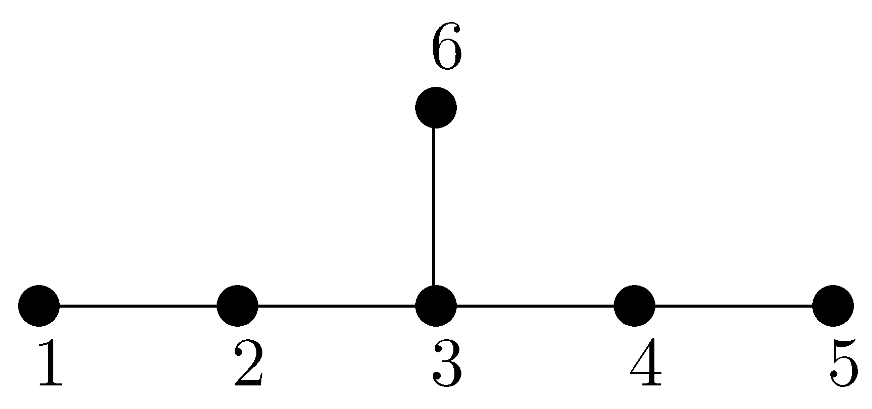
3.6. $E_6$ Algebra

Now we deal with the exceptional Lie algebra $E_6$. The matrix A is coinciding with the Cartan matrix (for $E_6$)

$$A=\left(A_{s{s}^{\prime }}\right)=\left(\begin{array}{cccccc}2& -1& 0& 0& 0& 0\\ -1& 2& -1& 0& 0& 0\\ 0& -1& 2& -1& 0& -1\\ 0& 0& -1& 2& -1& 0\\ 0& 0& 0& -1& 2& 0\\ 0& 0& -1& 0& 0& 2\end{array}\right).$$

(113)

This matrix is graphically depicted by the Dynkin diagram in Figure 5.

Figure 5. The Dynkin diagram for the Lie algebra $E_6$.

The inverse Cartan matrix for $E_6$

$$A^{-1}=\left(A^{s{s}^{\prime }}\right)=\left(\begin{array}{cccccc}\frac{4}{3}& \frac{5}{3}& 2& \frac{4}{3}& \frac{2}{3}& 1\\ \frac{5}{3}& \frac{10}{3}& 4& \frac{8}{3}& \frac{4}{3}& 2\\ 2& 4& 6& 4& 2& 3\\ \frac{4}{3}& \frac{8}{3}& 4& \frac{10}{3}& \frac{5}{3}& 2\\ \frac{2}{3}& \frac{4}{3}& 2& \frac{5}{3}& \frac{4}{3}& 1\\ 1& 2& 3& 2& 1& 2\end{array}\right)$$

(114)

implies due to (2)

$$(n_1,n_2,n_3,n_4,n_5,n_6)=(16,30,42,30,16,22).$$

(115)

For the Lie algebra $E_6$ we find the set of six fluxbrane polynomials [42], which are listed in Appendix B.

The polynomials have the following structure:

$$\begin{array}{c}{H}_1=1+16p_{1}z+120p_1{p}_2{z}^2+\cdots +120p_1^2{p}_2^3{p}_3^4{p}_4^2{p}_5{p}_6^2{z}^{14}\hfill \\ \hfill +16p_1^2{p}_2^3{p}_3^4{p}_4^3{p}_5{p}_6^2{z}^{15}+p_1^2{p}_2^3{p}_3^4{p}_4^3{p}_5^2{p}_6^2{z}^{16},\end{array}$$

$$\begin{array}{c}{H}_2=1+30p_{2}z+(120p_1{p}_2+315p_3{p}_2)z^2\hfill \\ \cdots +(120p_1^3{p}_2^6{p}_4^5{p}_5^2{p}_6^4{p}_3^8+315p_1^3{p}_2^6{p}_4^5{p}_5^3{p}_6^4{p}_3^7)z^{28}\\ \hfill +30p_1^3{p}_2^6{p}_3^8{p}_4^5{p}_5^3{p}_6^4{z}^{29}+p_1^3{p}_2^6{p}_3^8{p}_4^6{p}_5^3{p}_6^4{z}^{30},\end{array}$$

$$\begin{array}{c}{H}_3=1+42p_{3}z+(315p_2{p}_3+315p_4{p}_3+231p_6{p}_3)z^2\hfill \\ \cdots +(315p_1^4{p}_2^7{p}_4^8{p}_5^4{p}_6^6{p}_3^{11}+315p_1^4{p}_2^8{p}_4^7{p}_5^4{p}_6^6{p}_3^{11}+231p_1^4{p}_2^8{p}_4^8{p}_5^4{p}_6^5{p}_3^{11})z^{40}\\ \hfill +42p_1^4{p}_2^8{p}_3^{11}{p}_4^8{p}_5^4{p}_6^6{z}^{41}+p_1^4{p}_2^8{p}_3^{12}{p}_4^8{p}_5^4{p}_6^6{z}^{42},\end{array}$$

(116)

$$\begin{array}{c}{H}_4=1+30p_{4}z+(315p_3{p}_4+120p_5{p}_4)z^2\hfill \\ \cdots +(120p_1^2{p}_2^5{p}_4^6{p}_5^3{p}_6^4{p}_3^8+315p_1^3{p}_2^5{p}_4^6{p}_5^3{p}_6^4{p}_3^7)z^{28}\\ \hfill +30p_1^3{p}_2^5{p}_3^8{p}_4^6{p}_5^3{p}_6^4{z}^{29}+p_1^3{p}_2^6{p}_3^8{p}_4^6{p}_5^3{p}_6^4{z}^{30},\end{array}$$

$$\begin{array}{c}{H}_5=1+16p_{5}z+120p_4{p}_5{z}^2+\cdots +120p_1{p}_2^2{p}_3^4{p}_4^3{p}_5^2{p}_6^2{z}^{14}\hfill \\ \hfill +16p_1{p}_2^3{p}_3^4{p}_4^3{p}_5^2{p}_6^2{z}^{15}+p_1^2{p}_2^3{p}_3^4{p}_4^3{p}_5^2{p}_6^2{z}^{16},\end{array}$$

$$\begin{array}{c}{H}_6=1+22p_{6}z+231p_3{p}_6{z}^2+\cdots +231p_1^2{p}_2^4{p}_3^5{p}_4^4{p}_5^2{p}_6^3{z}^{20}\hfill \\ \hfill +22p_1^2{p}_2^4{p}_3^6{p}_4^4{p}_5^2{p}_6^3{z}^{21}+p_1^2{p}_2^4{p}_3^6{p}_4^4{p}_5^2{p}_6^4{z}^{22}.\end{array}$$

The powers of polynomials are in agreement with the relation (115). In what follows we denote

$$H_s=H_s\left(z\right)=H_s(z,\left(p_i\right)),$$

(117)

$s=1,\cdots ,6$; where $\left(p_i\right)=(p_1,p_2,p_3,p_4,p_5,p_6)$.

Due to (116) the asymptotical relations for the polynomials read as follows

$$H_s=H_s(z,\left(p_i\right))\sim \left(\prod _{l=1}^6{\left(p_l\right)}^{{\nu }^{sl}}\right)z^{n_s}\equiv H_s^{as}(z,\left(p_i\right)),$$

(118)

$s=1,\cdots ,6$, as $z\to \infty$. Here,

$$\nu =\left({\nu }^{sl}\right)=\left(\begin{array}{cccccc}2& 3& 4& 3& 2& 2\\ 3& 6& 8& 6& 3& 4\\ 4& 8& 12& 8& 4& 6\\ 3& 6& 8& 6& 3& 4\\ 2& 3& 4& 3& 2& 2\\ 2& 4& 6& 4& 2& 4\end{array}\right).$$

(119)

This matrix reads

$$\nu =A^{-1}(I+P),$$

(120)

where $A^{-1}$ is inverse Cartan matrix, I is $6\times 6$ identity matrix and

$$P=\left(\begin{array}{cccccc}0& 0& 0& 0& 1& 0\\ 0& 0& 0& 1& 0& 0\\ 0& 0& 1& 0& 0& 0\\ 0& 1& 0& 0& 0& 0\\ 1& 0& 0& 0& 0& 0\\ 0& 0& 0& 0& 0& 1\end{array}\right).$$

(121)

is permutation matrix. This matrix is related to the permutation $\sigma \in S_6$ ($S_6$ is symmetric group)

$$\sigma :(1,2,3,4,5,6)\mapsto (5,4,3,2,1,6),$$

(122)

by the following formula $P=\left(P_j^i\right)=\left({\delta }_{\sigma \left(j\right)}^i\right)$. Here, $\sigma$ is the generator of the group of symmetry of the Dynkin diagram $G=\{\sigma ,id\}$. (G is isomorphic to the group $Z_2$.) $\sigma$ is a composition of two transpositions: $(1\mapsto 5)$ and $(2\mapsto 4)$.

We note that the matrix $\nu$ is symmetric one and

$$\sum _{s=1}^6{\nu }^{sl}=n_l,$$

(123)

$l=1,\cdots ,6$.

Now we introduce the dual (ordered) set $\left({\widehat{p}}_i\right)=\left(p_{\sigma \left(i\right)}\right)$, $i=1,\cdots ,6$. By using the relations for polynomials from Appendix B we are led to the following two identities which are verified with the aid of MATHEMATICA.

3.6.1. Symmetry Relations

Proposition 10. 

For all $p_i$ and z

$$H_{\sigma \left(s\right)}(z,\left(p_i\right))=H_s(z,\left({\widehat{p}}_i\right)),$$

(124)

$s=1,\cdots ,6$.

3.6.2. Duality Relations

Proposition 11. 

For all $p_i>0$ and $z>0$

$$H_s(z,\left(p_i\right))=H_s^{as}(z,\left(p_i\right))H_s(z^{-1},\left({\widehat{p}}_i^{-1}\right)),$$

(125)

$s=1,\cdots ,6$.

The solution (8)–(10) reads in our case

$$\begin{array}{c}g=\left(\prod _{s=1}^6{H}_s^{2h/(D-2)}\right)\left\{d\rho \otimes d\rho +\left(\prod _{s=1}^6{H}_s^{-2h}\right){\rho }^{2}d\varphi \otimes d\varphi +g^2\right\},\end{array}$$

(126)

$$\begin{array}{c}exp\left({\phi }^a\right)=\prod _{s=1}^6{H}_s^{h{\lambda }_s^a},\end{array}$$

(127)

$$\begin{array}{c}{F}^s={\mathcal{B}}^s\rho d\rho \wedge d\varphi ,\end{array}$$

(128)

$a,s=1,\cdots ,6$, where $g^1=d\varphi \otimes d\varphi$ is a metric on $M_1=S^1$ ($0<\varphi <2\pi$), $g^2$ is a Ricci-flat metric on $M_2$ of signature $(-,+,\cdots ,+)$. Here,

$${\mathcal{B}}^s=-Q_s\left(\prod _{l=1}^6{H}_l^{-A_{sl}}\right)$$

(129)

and due to (14)–(16)

$$K=K_s=\frac{D-3}{D-2}+{\overrightarrow{\lambda }}_s^2,$$

(130)

$h_s=h=K^{-1}$,

$${\overrightarrow{\lambda }}_s{\overrightarrow{\lambda }}_{s^{\prime }}=\frac{1}{2}K{A}_{s{s}^{\prime }}-\frac{D-3}{D-2}\equiv G_{s{s}^{\prime }},$$

(131)

$s,s^{\prime }=1,\cdots ,6$.

3.7. Some Relations between Polynomials

Here, we denote the set of polynomials corresponding to a set of parameters $p_1>0$, …, $p_n>0$ as following

$$H_s=H_s(z,p_1,\dots ..,p_n;A),$$

(132)

$s=1,\cdots ,n$, where $A=A\left[\mathcal{G}\right]$ is the Cartan matrix corresponding to a (semi)simple Lie algebra $\mathcal{G}$ of rank n.

3.7.1. $C_{n+1}$-Polynomials from $A_{2n+1}$-Ones

It was conjectured in Ref. [28] that the set of polynomials corresponding to the Lie algebra $C_{n+1}$ may be obtained from the set of polynomials corresponding to the Lie algebra $A_{2n+1}$ according to the following relations

$$H_s(z,p_1,...,p_{n+1};A\left[C_{n+1}\right])=H_s(z,p_1,...,p_{n+1},p_{n+2}=p_n,...,p_{2n+1}=p_1;A\left[A_{2n+1}\right]),$$

(133)

$s=1,\cdots ,n+1$, i.e., the parameters $p_1,...,p_{n+1},p_{n+2},...,p_{2n+1}$ are identified symmetrically with respect to $p_{n+1}$.

Relation (133) may be readily verified at least for $n=1,2$ by using explicit relations for corresponding polynomials presented above.

3.7.2. $B_n$-Polynomials from $D_{n+1}$-Ones

Due to the conjecture from Ref. [28], the set polynomials corresponding to the Lie algebra $B_n$ can be obtained from the set of polynomials corresponding to the Lie algebra $D_{n+1}$ according to the following relation

$$H_s(z,p_1,...,p_n;A\left[B_n\right])=H_s(z,p_1,...,p_n,p_{n+1}=p_n;A\left[D_{n+1}\right]),$$

(134)

$s=1,\cdots ,n$, i.e., the parameters $p_n$ and $p_{n+1}$ are identified.

Relation (134) can be readily verified at least for $n=3,4$ by using explicit relations for corresponding polynomials presented above.

3.7.3. $G_2$-Polynomials from $D_4$-Ones

It can be readily checked that $G_2$-polynomials may be obtained just by imposing the following relations on parameters of $D_4$-polynomials: $p_1=p_3=p_4$. We obtain

$$\begin{array}{c}\hfill H_1(z,p_1,p_2,p_1,p_1;A\left[D_4\right])=H_1(z,p_1,p_2;A\left[G_2\right]),\end{array}$$

(135)

$$\begin{array}{c}\hfill H_2(z,p_1,p_2,p_1,p_1;A\left[D_4\right])=H_2(z,p_1,p_2;A\left[G_2\right]).\end{array}$$

(136)

It looks like we glue the symmetric points (1, 3 and 4) at the Dynkin graph for $D_4$ algebra (see Figure 3) in order to obtain the Dynkin graph for $G_2$ algebra (see Figure 1).

3.7.4. $F_4$-Polynomials from $E_6$-Ones

It can be verified that $F_4$-polynomials may be obtained by imposing the following relations on parameters of $E_6$-polynomials: $p_1=p_5={\overline{p}}_4$, $p_2=p_4={\overline{p}}_3$, $p_3={\overline{p}}_2$, $p_6={\overline{p}}_1$. We obtain

$$\begin{array}{c}\hfill H_1(z,p_1,p_2,p_3,p_2,p_1,p_6;A\left[E_6\right])=H_4(z,{\overline{p}}_1,{\overline{p}}_2,{\overline{p}}_3,{\overline{p}}_4;A\left[F_4\right]),\end{array}$$

(137)

$$\begin{array}{c}\hfill H_2(z,p_1,p_2,p_3,p_2,p_1,p_6;A\left[E_6\right])=H_3(z,{\overline{p}}_1,{\overline{p}}_2,{\overline{p}}_3,{\overline{p}}_4;A\left[F_4\right]),\end{array}$$

(138)

$$\begin{array}{c}\hfill H_3(z,p_1,p_2,p_3,p_2,p_1,p_6;A\left[E_6\right])=H_2(z,{\overline{p}}_1,{\overline{p}}_2,{\overline{p}}_3,{\overline{p}}_4;A\left[F_4\right]),\end{array}$$

(139)

$$\begin{array}{c}\hfill H_6(z,p_1,p_2,p_3,p_2,p_1,p_6;A\left[E_6\right])=H_1(z,{\overline{p}}_1,{\overline{p}}_2,{\overline{p}}_3,{\overline{p}}_4;A\left[F_4\right]).\end{array}$$

(140)

It looks like we glue the symmetric points (1 and 5, 2 and 4) at the Dynkin graph for $E_6$ algebra (see Figure 5) in order to obtain the Dynkin graph for $F_4$ algebra (see Figure 3).

3.7.5. Reduction Formulas

Here, we denote the Cartan matrix in the following way: $A=A_{\mathsf{\Gamma }}$, where $\mathsf{\Gamma }$ is the related Dynkin graph. Let i be a node of $\mathsf{\Gamma }$. We denote by ${\mathsf{\Gamma }}_i$ a Dynkin graph (which corresponds to a certain semi-simple Lie algebra) that is obtained from $\mathsf{\Gamma }$ by erasing all lines that have endpoints at i. It can be verified (e.g., by using MATHEMATICA) that for the polynomials presented above the following reduction formulae hold

$$H_s(z,p_1,...,p_i=0,...,p_n;A_{\mathsf{\Gamma }})=H_s(z,p_1,...,p_{i-1},p_{i+1},...,p_n;A_{{\mathsf{\Gamma }}_i}),$$

(141)

$s=1,\cdots ,i-1,i+1,\cdots ,n$, and

$$H_i(z,p_1,...,p_i=0,...,p_n;A_{\mathsf{\Gamma }})=1.$$

(142)

This means that by setting $p_i=0$ we reduce the set of polynomials by replacing the Cartan matrix $A_{\mathsf{\Gamma }}$ with the Cartan matrix $A_{{\mathsf{\Gamma }}_i}$. In this case the polynomial $H_i=1$ corresponds to $A_1$-subalgebra (represented by the node i) and the parameter $p_i=0$.

As an example of reduction formulas we present the following relations

$$H_s(z,p_1,...,p_n,p_{n+1}=0;A\left[\mathcal{G}\right])=H_s(z,p_1,...,p_n;A\left[A_n\right]),$$

(143)

$s=1,\cdots ,n$, for $\mathcal{G}=A_{n+1},B_{n+1},C_{n+1},D_{n+1}$ with suitable restrictions on n. These relations are valid at least for all $ABCD$-polynomials presented above. In writing relation (141) we use the numbering of the nodes in accordance with the Dynkin diagrams shown in the figures presented above.

The reduction formulas (142) for $A_5$-polynomials with $p_3=0$ are shown in Figure 6. The reduced polynomials coincide with those corresponding to semisimple Lie algebra $A_2⨁A_1⨁A_2$.

Figure 6. Dynkin diagram for semisimple Lie algebra $A_2⨁A_1⨁A_2$ describing the set of $A_5$-polynomials with $p_3=0$ [28].

4. Flux Integrals

As in the previous section, we deal here with the solution (8)–(10) with $n=l$, $w=+1$ and $M_1=S^1$ and $h_{\alpha \beta }={\delta }_{\alpha \beta }$.

We denote $\left({\lambda }_{sa}\right)=\left({\lambda }_s^a\right)={\overrightarrow{\lambda }}_s$, $s=1,\cdots ,n$. The solution corresponds to a simple finite-dimensional Lie algebra $\mathcal{G}$, i.e., the matrix $A=\left(A_{s{s}^{\prime }}\right)$ is coinciding with the Cartan matrix of this Lie algebra.

In this case, we get relations (17), (18) for $h_s=K_s^{-1}>0$ and scalar products ${\overrightarrow{\lambda }}_s{\overrightarrow{\lambda }}_l$ which follow from (14)–(16).

Due to (14)–(16) that

$$\frac{h_i}{h_j}=\frac{K_j}{K_i}=\frac{B_{jj}}{B_{ii}}=\frac{B_{ji}}{B_{ii}}\frac{B_{jj}}{B_{ij}}=\frac{A_{ji}}{A_{ij}}$$

(144)

for any $i\ne j$ obeying $A_{ij}=A_{ji}\ne 0$; $i,j=1,\cdots ,n$.

It follows from (144) and the connectedness of the Dynkin diagram for a simple Lie algebra that

$$\frac{h_i}{h_j}=\frac{K_j}{K_i}=\frac{r_j}{r_i}$$

(145)

$i\ne j$, where $r_i=({\alpha }_i,{\alpha }_i)$ is length squared of a simple root ${\alpha }_i$ of the Lie algebra $\mathcal{G}$. Here, ($(.,.)$ is dual Killing–Cartan form and

$$A_{ij}=2({\alpha }_i,{\alpha }_j)/({\alpha }_j,{\alpha }_j),$$

(146)

$i,j=1,\cdots ,n$. Due to (145) we obtain

$$K_i=\frac{1}{2}K{r}_i,$$

(147)

$i=1,\cdots ,n$, where $K>0$.

Now we consider the oriented 2-dimensional manifold $M_{*}=(0,+\infty )\times S^1$. The flux integrals read

$${\mathsf{\Phi }}^s={\int }_{M_{*}}{F}^s={\int }_0^{+\infty }d\rho {\int }_0^{2\pi }d\varphi \rho {\mathcal{B}}^s\left({\rho }^2\right)=2\pi {\int }_0^{+\infty }d\rho \rho {\mathcal{B}}^s\left({\rho }^2\right),$$

(148)

where

$${\mathcal{B}}^s\left({\rho }^2\right)=q_s\prod _{l=1}^n{\left(H_l\left({\rho }^2\right)\right)}^{-A_{sl}}.$$

(149)

Due to (13) and (19) we have

$$p_s=\frac{P_s}{n_s}=\frac{K_s}{4n_s}{q}_s^2.$$

(150)

The integrals (148) are convergent for all $s=1,\cdots ,n$, if the conjecture on polynomial structure of moduli functions $H_s$ is satisfied for the Lie algebra $\mathcal{G}$ under consideration.

Indeed, polynomial assumption (1) implies

$$H_s\left({\rho }^2\right)\sim C_s{\rho }^{2n_s},C_s=P_s^{\left(n_s\right)},$$

(151)

as $\rho \to +\infty$; $s=1,\cdots ,n$. From (149), (151) and the identities ${\sum }_1^n{A}_{sl}{n}_l=2$, following from (2), we obtain

$${\mathcal{B}}^s\left({\rho }^2\right)\sim q_s{C}^s{\rho }^{-4},C^s=\prod _{l=1}^n{C}_l^{-A_{sl}}.$$

(152)

Hence the integral (148) is convergent for any $s=1,\cdots ,n$.

From master Equation (11), we obtain

$$\begin{array}{c}\hfill {\int }_0^{+\infty }d\rho \rho {\mathcal{B}}^s\left({\rho }^2\right)=q_s{P}_s^{-1}\frac{1}{2}{\int }_0^{+\infty }dz\frac{d}{dz}\left(\frac{z}{H_s}\frac{d}{dz}{H}_s\right)\\ \hfill =\frac{1}{2}{q}_s{P}_s^{-1}\underset{z\to +\infty }{lim}\left(\frac{z}{H_s}\frac{d}{dz}{H}_s\right)=\frac{1}{2}{n}_s{q}_s{P}_s^{-1},\end{array}$$

(153)

which implies (see (13)) [43]

$${\mathsf{\Phi }}^s=4\pi n_s{q}_s^{-1}{h}_s,$$

(154)

$s=1,\cdots ,n$.

Thus, we see that any flux ${\mathsf{\Phi }}^s$ depends only upon one integration constant $q_s\ne 0$. This is a nontrivial fact since the integrand form $F^s$ depends upon all constants: $q_1,\cdots ,q_n$.

It should be noted that, for $D=4$ and $g^2=-dt\otimes dt+dx\otimes dx$, $q_s$ is coinciding with the value of the x-component of the magnetic field on the axis of symmetry.

For the case of Gibbons–Maeda dilatonic generalization of the Melvin solution, corresponding to $D=4$, $n=l=1$ and $\mathcal{G}=A_1$ [6], the flux from (154) ($s=1$) is in agreement with that obtained in Ref. [26]. For the Melvin’s solution and some higher dimensional extensions (with $\mathcal{G}=A_1$) see also Ref. [15].

Owing to (145) the ratios

$$\frac{q_i{\mathsf{\Phi }}^i}{q_j{\mathsf{\Phi }}^j}=\frac{n_i{h}_i}{n_j{h}_j}=\frac{n_i{r}_j}{n_j{r}_i}$$

(155)

are just fixed numbers which depend upon the Cartan matrix $\left(A_{ij}\right)$ of a simple finite-dimensional Lie algebra $\mathcal{G}$.

Since the manifold $M_{*}=(0,+\infty )\times S^1$ is isomorphic to the manifold ${\mathbb{R}}_{*}^2={\mathbb{R}}^2\setminus \left\{0\right\}$, the solution (8)–(10) may be rewritten (by pull-backs) onto manifold ${\mathbb{R}}_{*}^2\times M_2$. In this new presentation of the solution coordinates $\rho$, $\varphi$ are understood as polar coordinates on ${\mathbb{R}}_{*}^2$. Since they are not globally defined one may consider two charts with coordinates $\rho$, $\varphi ={\varphi }_1$ and $\rho$, $\varphi ={\varphi }_2$, where $\rho >0$, $0<{\varphi }_1<2\pi$ and $-\pi <{\varphi }_2<\pi$. Here, $exp\left(i{\varphi }_1\right)=exp\left(i{\varphi }_2\right)$. For both charts we have $x=\rho cos\varphi$ and $y=\rho sin\varphi$, where $x,y$ are standard (Euclidean) coordinates of ${\mathbb{R}}^2$. By using the identity $\rho d\rho \wedge d\varphi =dx\wedge dy$ we obtain

$$F^s=q_s\prod _{l=1}^n{\left(H_l(x^2+y^2)\right)}^{-A_{sl}}dx\wedge dy,$$

(156)

$s=1,\cdots ,n$.

Now, let us show that 2-forms (156) are well-defined on ${\mathbb{R}}^2$. Indeed, due to conjecture from Ref. [3] any polynomial $H_s\left(z\right)$ is a smooth function on $\mathbb{R}=(-\infty ,+\infty )$ obeying $H_s\left(z\right)>0$ for $z\in (-{\epsilon }_s,+\infty )$, where ${\epsilon }_s>0$. This is so since due to polynomial conjecture from Ref. [3] we have $H_s\left(z\right)>0$ for $z>0$ and $H_s(+0)=1$. Hence, $\left({\prod }_{l=1}^n{\left(H_l(x^2+y^2)\right)}^{-A_{sl}}\right)$ is a smooth function since it is just a composition of two well-defined smooth functions: $\left({\prod }_{l=1}^n{\left(H_l\left(z\right)\right)}^{-A_{sl}}\right)$ and $z=x^2+y^2$.

Now, we show that there exist 1-forms $A^s$ obeying $F^s=d{A}^s$ which are globally defined on ${\mathbb{R}}^2$. Let us consider the open submanifold ${\mathbb{R}}_{*}^2$. The 1-forms

$$A^s=\left({\int }_0^{\rho }d\overline{\rho }\overline{\rho }{\mathcal{B}}^s\left({\overline{\rho }}^2\right)\right)d\varphi =\frac{1}{2}\left({\int }_0^{{\rho }^2}d\overline{z}{\mathcal{B}}^s\left(\overline{z}\right)\right)d\varphi$$

(157)

are well defined on ${\mathbb{R}}_{*}^2$ and obey $F^s=d{A}^s$, $s=1,\cdots ,n$. It is obvious that here

$$d\varphi ={(x^2+y^2)}^{-1}(-ydx+xdy).$$

(158)

It follows from the master Equation (11) that

$$\begin{array}{c}\hfill A^s=\frac{q_s}{2P_s}\left({\int }_0^{{\rho }^2}d\overline{z}\frac{d}{d\overline{z}}\left(\frac{\overline{z}}{H_s\left(\overline{z}\right)}\frac{d}{d\overline{z}}{H}_s\left(\overline{z}\right)\right)\right)d\varphi \\ \hfill =\frac{2h_s}{q_s}\frac{H_s^{{}^{\prime }}\left({\rho }^2\right)}{H_s\left({\rho }^2\right)}{\rho }^{2}d\varphi ,\end{array}$$

(159)

$s=1,\cdots ,n$. Here, $H{{}^{\prime }}_s=\frac{d}{dz}{H}_s$. Due to relation ${\rho }^{2}d\varphi =-ydx+xdy$, we obtain

$$A^s=\frac{2h_s}{q_s}\frac{H_s^{{}^{\prime }}(x^2+y^2)}{H_s(x^2+y^2)}(-ydx+xdy),$$

(160)

$s=1,\cdots ,n$. Thus, we are led to 1-forms (160) which are well-defined (smooth) 1-forms on ${\mathbb{R}}^2$.

It should be noted that in case of Gibbons–Maeda solution [6] (with $D=4$, $n=l=1$ and $\mathcal{G}=A_1$) the gauge potential from (159) coincides (up to notations) with that considered in Ref. [8].

Now we verify the formula (154) for flux integrals by using the relation (160) for 1-forms $A^s$. Let us consider a $2d$ oriented manifold (disk)

$$D_R=\{(x,y):x^2+y^2\le R^2\}$$

(161)

with the boundary

$$\partial D_R=C_R=\{(x,y):x^2+y^2=R^2\}.$$

(162)

Here, $C_R$ is a circle of radius R. It is just an $1d$ oriented manifold with the orientation (inherited from that of $D_R$) obeying the relation ${\int }_{C_R}d\varphi =2\pi$. Using the Stokes–Cartan theorem we obtain

$${\mathsf{\Phi }}^s\left(R\right)={\int }_{D_R}{F}^s={\int }_{D_R}d{A}^s={\int }_{C_R}{A}^s=\frac{4\pi h_s}{q_s}\frac{H_s^{{}^{\prime }}\left(R^2\right)}{H_s\left(R^2\right)}{R}^2,$$

(163)

$s=1,\cdots ,n$. By using the asymptotic relation (151) we get

$$\underset{R\to +\infty }{lim}{\mathsf{\Phi }}^s\left(R\right)=\underset{R\to +\infty }{lim}{\int }_{D_R}{F}^s=\frac{4\pi h_s{n}_s}{q_s}={\mathsf{\Phi }}^s,$$

(164)

$s=1,\dots ,n$, in agreement with (154).

We note that, according to the definition of Abelian Wilson loop (factor), we have

$$W^s\left(C_R\right)=exp\left(i{\int }_{C_R}{A}^s\right)=exp\left(i{\mathsf{\Phi }}^s\left(R\right)\right),$$

(165)

$s=1,\dots ,n$. As a consequence (see (164)), we obtain finite limits

$$\underset{R\to +\infty }{lim}{W}^s\left(C_R\right)=exp\left(i{\mathsf{\Phi }}^s\right),$$

(166)

$s=1,\dots ,n$.

Finally, we note that the metric and scalar fields for our solution with $w=+1$ and $l=n$ can be extended to the manifold ${\mathbb{R}}^2\times M_2$.

Indeed, in standard $x,y$ coordinates on ${\mathbb{R}}^2$ the metric (8) and scalar fields (9) read as follows [43]

$$\begin{array}{c}\hfill g=\left(\prod _{s=1}^n{H}_s^{2h_s/(D-2)}\right)\left\{dx\otimes dx+dy\otimes dy+F{(-ydx+xdy)}_{\otimes }^2+g^2\right\},\end{array}$$

(167)

$$\begin{array}{c}\hfill {\phi }^a=\sum _{s=1}^n{h}_s{\lambda }_s^{a}ln{H}_s,\end{array}$$

(168)

$a=1,\cdots ,n$. Here, $H_s=H_s(x^2+y^2)$, $s=1,\cdots ,n$, ${\omega }_{\otimes }^2=\omega \otimes \omega$ and $F=F(x^2+y^2)$, where

$$F\left(z\right)=\left(\left(\prod _{s=1}^n{\left(H_s\left(z\right)\right)}^{-2h_s}\right)-1\right)z^{-1},$$

(169)

for $z\ne 0$ and

$$F\left(0\right)=\underset{z\to 0}{lim}F\left(z\right)=\sum _{s=1}^n(-2h_s{p}_s).$$

(170)

The metric and scalar fields are smooth on the manifold ${\mathbb{R}}^2\times M_2$ [43].

5. Dilatonic Black Holes

Relations on dilatonic coupling vectors (14)–(16) also appear for dilatonic black hole (DBH) solutions defined on the manifold

$$M=(R_0,+\infty )\times (M_0=S^2)\times (M_1=\mathbb{R})\times M_2,$$

(171)

where $R_0=2\mu >0$ and $M_2$ is a Ricci-flat manifold. These DBH solutions on M from (171) for the model under consideration may be extracted just from more general black brane solutions, see Refs. [35,36,44]. They read:

$$\begin{array}{c}\hfill g=\left(\prod _{s=1}^n{\mathbf{H}}_s^{2h_s/(D-2)}\right)\left\{f^{-1}dR\otimes dR+R^2{g}^0-\left(\prod _{s=1}^n{\mathbf{H}}^{-2h_s}\right)fdt\otimes dt+g^2\right\},\end{array}$$

(172)

$$\begin{array}{c}\hfill exp\left({\phi }^a\right)=\prod _{s=1}^n{\mathbf{H}}^{h_s{\lambda }_s^a},\end{array}$$

(173)

$$\begin{array}{c}\hfill F^s=-Q_s{R}^{-2}\left(\prod _{l=1}^n{\mathbf{H}}_l^{-A_{sl}}\right)dR\wedge dt,\end{array}$$

(174)

$s,a=1,\cdots ,n$, where $f=1-2\mu R^{-1}$, $g^0$ is the standard metric on $M_0=S^2$ and $g^2$ is a Ricci-flat metric of signature $(+,\cdots ,+)$ on $M_2$. Here, $Q_s\ne 0$ are integration constants (charges).

The functions ${\mathbf{H}}_s={\mathbf{H}}_s\left(R\right)>0$ obey the master equations

$$R^2\frac{d}{dR}\left(f\frac{R^2}{{\mathbf{H}}_s}\frac{d}{dR}{\mathbf{H}}_s\right)=B_s\prod _{l=1}^n{\mathbf{H}}_l^{-A_{sl}},$$

(175)

with the following boundary conditions (on the horizon and at infinity) imposed:

$${\mathbf{H}}_s(R_0+0)={\mathbf{H}}_{s0}>0,{\mathbf{H}}_s(+\infty )=1,$$

(176)

where

$$B_s=-K_s{Q}_s^2,$$

(177)

$s=1,\cdots ,n$.

It was shown in Ref. [36] that these polynomials may be obtained (at least for small enough $Q_s$) from fluxbrane polynomials $H_s\left(z\right)$ presented in this paper.

Indeed, let us denote $f=f\left(z\right)=1-2\mu z$, $z=1/R$. Then, the relations (175) may be rewritten as follows

$$\frac{d}{df}\left(\frac{f}{{\mathbf{H}}_s}\frac{d}{df}{\mathbf{H}}_s\right)=B_s{\left(2\mu \right)}^{-2}\prod _{l=1}^n{\mathbf{H}}_l^{-A_{sl}},$$

(178)

$s=1,\cdots ,n$. These relations could be solved (at least for small enough $Q_s$) by using fluxbrane polynomials $H_s\left(f\right)=H_s(f;p)$, given by $n\times n$ Cartan matrix $\left(A_{sl}\right)$, where $p=(p_1,\cdots ,p_n)$ is the set of parameters [36]. Here we impose the restrictions $p_s\ne 0$ for all s.

Due to approach of Ref. [36] we put

$${\mathbf{H}}_s\left(z\right)=H_s(f\left(z\right);p)/H_s(1;p)$$

(179)

for $s=1,\cdots ,n$. Then, the relations (178), are satisfied identically if [36]

$$n_s{p}_s\prod _{l=1}^n{\left(H_l(1;p)\right)}^{-A_{sl}}=B_s/{\left(2\mu \right)}^2,$$

(180)

$s=1,\dots ,n$.

We call the set of parameters $p=(p_1,\cdots ,p_n)$ ($p_i\ne 0$) a proper one if [36]

$$H_s(f;p)>0$$

(181)

for all $f\in [0,1]$ and $s=1,\cdots ,n$. Here, we consider only proper p. Due to relations (180) and $B_s<0$, we have $p_s<0$ for all $s=1,\cdots ,n$, i.e., one should use fluxbrane polynomials with negative parameters $p_s$ for a description of black hole solutions under consideration.

The boundary conditions (176) are valid, since

$${\mathbf{H}}_s({\left(2\mu \right)}^{-1}-0)=1/H_s(1;p)>0,$$

(182)

$s=1,\cdots ,n$ (see definition (179)).

For small enough $p_i$, the set $(p_1,\cdots ,p_n)$ is proper and relation (180) defines one-to-one correspondence between the sets of parameters $(p_1,\cdots ,p_n)$ and $(Q_1^2,\cdots ,Q_n^2)$.

Relations (182) imply the following formula for the Hawking temperature [36]

$$T_H=\frac{1}{8\pi \mu }\prod _{s=1}^n{\left(H_s(1;p)\right)}^{h_s}.$$

(183)

It should be noted that fluxbrane polynomials were used in Refs. [45,46,47] in the context of dyon-like black hole solutions. (To a certain extent these papers were inspired by Ref. [48].)

6. Conclusions

Here, we have explored a multidimensional generalization of the Melvin’s solution corresponding to a simple finite-dimensional Lie algebra $\mathcal{G}$. It takes place in a D-dimensional model which contains metric n Abelian 2-forms $F^s=d{A}^s$ and $l\ge n$ scalar fields ${\phi }^{\alpha }$. (Here, we have put $l=n$ for simplicity.)

The solution is governed by a set of n moduli functions $H_s\left(z\right)$, $s=1,\cdots ,n$, which were assumed earlier to be polynomials—so-called fluxbrane polynomials. These polynomials define special solutions to open Toda chain equations corresponding to the Lie algebra $\mathcal{G}$. The polynomials $H_s\left(z\right)$ also depend upon parameters $p_s\sim q_s^2$, where $q_s$ are coinciding for $D=4$ (up to a sign) with the values of colored magnetic fields on the axis of symmetry.

Here, we have presented examples of polynomials corresponding to Lie algebras of rank $r=1,2,3,4,5$ and exceptional Lie algebra $E_6$ and have outlined the symmetry and duality relations for these polynomials. The so-called duality relations for fluxbrane polynomials describe a behavior of the solutions under the inversion: $\rho \to 1/\rho$, which makes the model in tune with so-called T-duality in string models. These relations can be also mathematically understood in terms of the discrete groups of symmetry of Dynkin diagrams for the corresponding Lie algebras.

We have presented calculations of $2d$ flux integrals ${\mathsf{\Phi }}^s=\int F^s$, where $F^s$ are 2-forms, $s=1,\cdots ,n$. It is remarkable that any flux ${\mathsf{\Phi }}^s$ depends only upon one parameter $q_s$, while the integrand $F^s$ depends upon all parameters $q_1,\cdots ,q_n$.

Here, we have also outlined possible applications of fluxbrane polynomials for seeking dilatonic black hole solutions (e.g., $4d$ ones) in the model under consideration.

It should be noted that fluxbrane polynomials may also describe certain subclass of self-dual solutions to Yang-Mills equations in a flat space of signature $(+,+,-,-)$ [49]. This subclass belong to a more general Toda chain class of self-dual solutions.

Here, an interesting question occurs: how can the nice properties of polynomials (symmetries, duality relations, reduction formulas) be used for a description of geometries of Melvin-like solutions (and other fluxbrane ones) and possible generating of new solutions? This and other related questions may be a subject of future publications.