Chaotification of 1D Maps by Multiple Remainder Operator Additions—Application to B-Spline Curve Encryption

Abstract

In this work, a chaotification technique is proposed for increasing the complexity of chaotic maps. The technique consists of adding the remainder of multiple scalings of the map’s value for the next iteration, so that the most- and least-significant digits are combined. By appropriate parameter tuning, the resulting map can achieve a higher Lyapunov exponent value, a result that was first proven theoretically and then showcased through numerical simulations for a collection of chaotic maps. As a proposed application of the transformed maps, the encryption of B-spline curves and patches was considered. The symmetric encryption consisted of two steps: a shuffling of the control point coordinates and an additive modulation. A transformed chaotic map was utilised to perform both steps. The resulting ciphertext curves and patches were visually unrecognisable compared to the plaintext ones and performed well on several statistical tests. The proposed work gives an insight into the potential of the remainder operator for chaotification, as well as the chaos-based encryption of curves and computer graphics.

1. Introduction

1.1. Applications of Chaos and Chaotification

The applications of chaos in the digital world have been reported in multiple works [1,2,3,4] and span the areas of computing, encryption, surveillance, communications, fingerprinting, and many more. Within the broad range of these applications, both continuous and discrete chaotic systems are considered, depending on the application at hand.

Continuous chaotic systems have many merits, such as more degrees of freedom and a higher state space. However, this comes at the cost of computational time, which may pose problems in applications where execution time is of the essence. They are also heavily dependent on the numerical method used to compute their solution, which creates issues of reproducibility across different computers and digital devices.

This is why it is more suitable to consider discrete-time chaotic systems, or chaotic maps as they are also termed. Discrete maps can achieve chaotic behaviour even in a single dimension, have a much lighter computational cost, and are solved iteratively, so they are not dependent on numerical integration methods.

Still, for both continuous and discrete systems, there are several features that need to be present, in order to make a chaotic system suitable for use in security-related applications, such as encryption, watermarking, surveillance, and others. Desirable features include the absence of parameter ranges that lead to periodic behaviour and an increased sensitivity to the initial conditions, indicated by high Lyapunov exponent values, a high key space, and an unrecognisable phase diagram with no visual structure. These are all attributes of maps with increased complexity. The pursuit of finding such maps led to the field of study known as chaotification, which in general refers to the problem of constructing novel chaotic maps or devising methods to modify known maps in order to satisfy the above properties. Since there is already an abundance of chaotic maps in the literature, chaotification usually does not involve the generation of novel maps, but techniques that can be applied to any known map to improve its performance in cryptographic and similar tasks.

The field of chaotification is very active at the moment, with numerous contributions. Popular techniques include the use of sinusoidal functions [5,6,7,8,9,10,11,12], exponential terms [13], piecewise maps [14,15], the modulo operator [7,16,17,18,19], the coupling of maps [20], the composition through internal perturbation [21], and others [22,23].

In [18], the authors proposed a chaotification technique that consisted of adding a remainder term to any 1D map, in order to mix the most- and least-significant digits in each iteration and boost the chaotic behaviour of the seed map. Indeed, it was shown that, by the appropriate parameter choice, the Lyapunov exponent of the modified map can be larger than that of the seed map. Moreover, the modified map showed wide areas of uninterrupted chaotic behaviour in its parameter space. The present work is a straightforward extension of the chaotification technique in [18] by using a summation of remainder operators. The transformed maps are then considered for the encryption of B-spline curves and patches.

1.2. Encryption

The principles of chaos-based encryption are applicable to any type of data and, so far, have indeed been applied to the encryption of images [11,12,24,25], text [25], and continuous signals [26]. Image encryption seems to be the most-popular application, mainly due to its visual aspect, which makes it easier to depict and compare plaintext and ciphertext data and interpret the results of the various statistical tests performed on them.

In addition to the above, recently, there has been an increasing interest in encrypting 3D objects. Three-dimensional graphics can represent any type of data, from mechanical and biological objects, to video game graphics [27,28,29]. The format used to represent such graphics is the stereolithography (STL) format. In this work, in order to complement the work on computer graphics encryption, B-spline curves and patches will be chosen as the plaintext data.

B-spline curves, and their simpler form, Bézier curves, are a well-established family of parametric curves, which are extensively used for modelling 2D and 3D graphics [30,31,32,33,34,35,36]. Their use originated in the automotive industry, but currently, their usage has been expanded to a plethora of applications, most notably graphic design, robotics, and navigation, as they can be used to effectively generate motion trajectories for a robotic manipulator, a UVG, or a UAV.

There are several properties that make B-spline curves so useful. First is the ease of their implementation, as they are simply described by a closed-form formula. That formula requires only the specification of a set of control points characterising the shape of the curve. These points also define the convex hull of the curve, so it is easy to specify its boundaries, making it easier to avoid intersections with obstacles. Another property is that they are locally controllable, meaning that changing a single control point of the B-spline will affect only a part of the curve. Finally, their smoothness can also be controlled by choosing the appropriate curve order and control point placement.

In this work, a symmetric encryption technique of B-spline curves and patches was considered, which consists of two separate steps. The first step involves the shuffling of the control points, by the application of a chaotic pseudorandom rule. The second consists of combining the control points with the values of a transformed chaotic map, to mask their value. The resulting ciphertext curves were visually unrecognisable and also performed well on several statistical tests. This technique complements previous works that considered the encryption of 3D objects and proposes a setup for encrypting parametric curves.

The main contributions of this work is the construction and analysis of mappings using multiple remainder operators and the presentation of a new B-spline encryption algorithm. The use of multiple remainder operators can efficiently mix the least- and most-significant digits between iterative mappings and can be further explored and modified in the future. The encryption of B-spline curves using a two-step process can be a starting point for further experimentation into encrypting geometrical data structures in general.

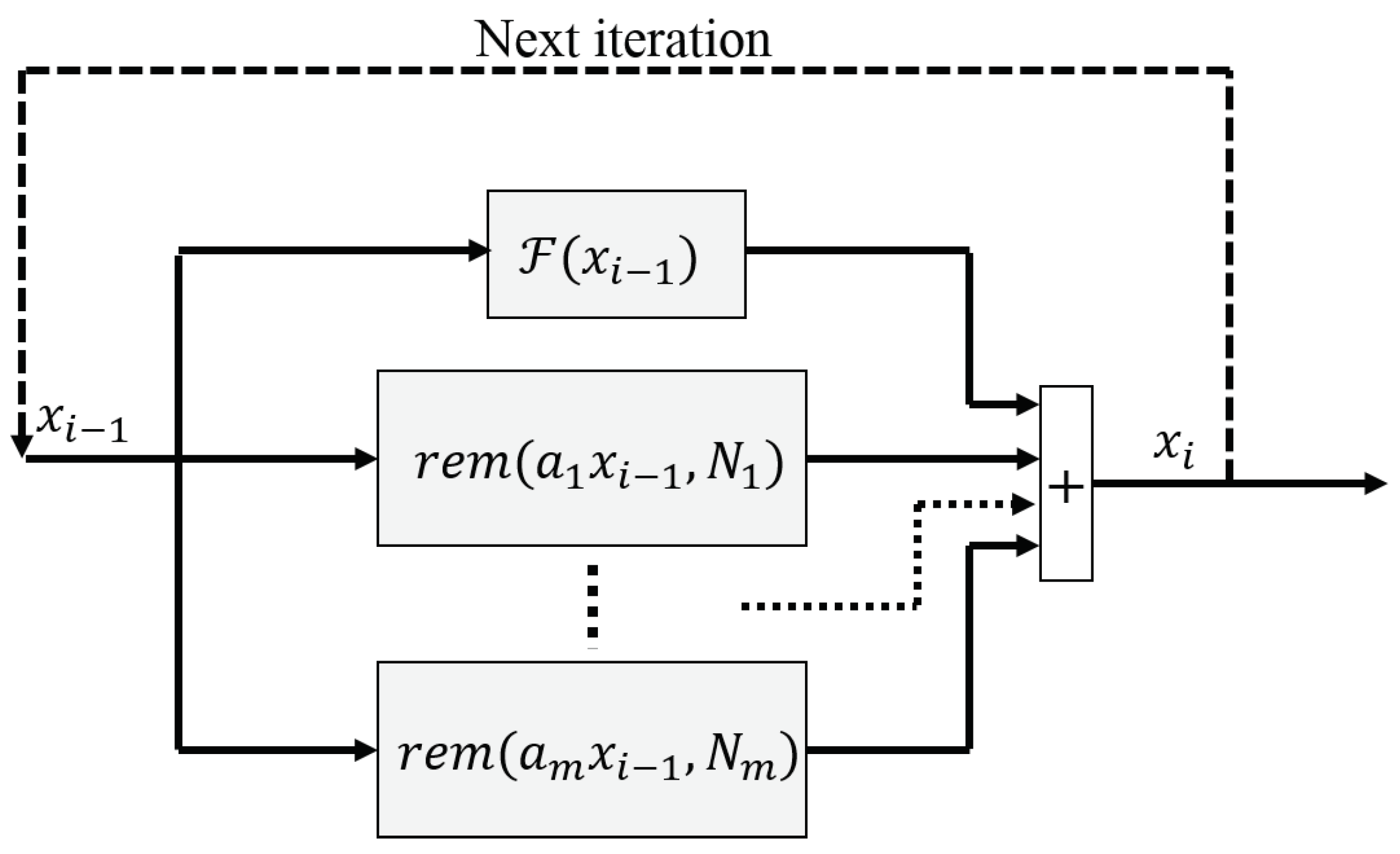
The rest of the work is structured as follows. In Section 2, the proposed chaotification technique is introduced. In Section 3, the technique is applied to several known maps. In Section 4, the effect of the proposed chaotification technique in expanding the key space of the resulting encryption protocol is discussed. In Section 5, the computational cost of applying the technique is presented. In Section 6 and Section 7, the symmetric encryption of B-spline curves and surfaces is considered. The simulation results of encryption are shown in Section 8. Finally, Section 9 concludes the present work and discusses topics for future research.

2. The Proposed Chaotification Technique

Consider a one-dimensional discrete time map described by the iterative formula:

$$x_i=\mathcal{F}\left(x_{i-1}\right).$$

(1)

The proposed chaotification technique is an extension of [18] and consists of using the remainder operator to add multiple scalings of the map’s value $x_{i-1}$ into the next iteration $x_i$ as follows:

$$x_i={\mathcal{H}}_m\left(x_{i-1}\right)=\mathcal{F}\left(x_{i-1}\right)+\sum _{j=1}^{m}rem(a_j{x}_{i-1},N_j),$$

(2)

where $a_j>0$ are the control parameters, $N_j\in {\mathbb{R}}_{\ast }^{+}$ map the remainder result on the interval $(-N_j,N_j)$, and $m\in \mathbb{N}$. The technique is also illustrated in Figure 1.

Theorem 1. 

Let

$${\mathcal{H}}_m\left(x_i\right)=\mathcal{F}\left(x_i\right)+\sum _{j=1}^{m}rem(a_j{x}_i,N_j).$$

(3)

Then, the following hold:

1. 

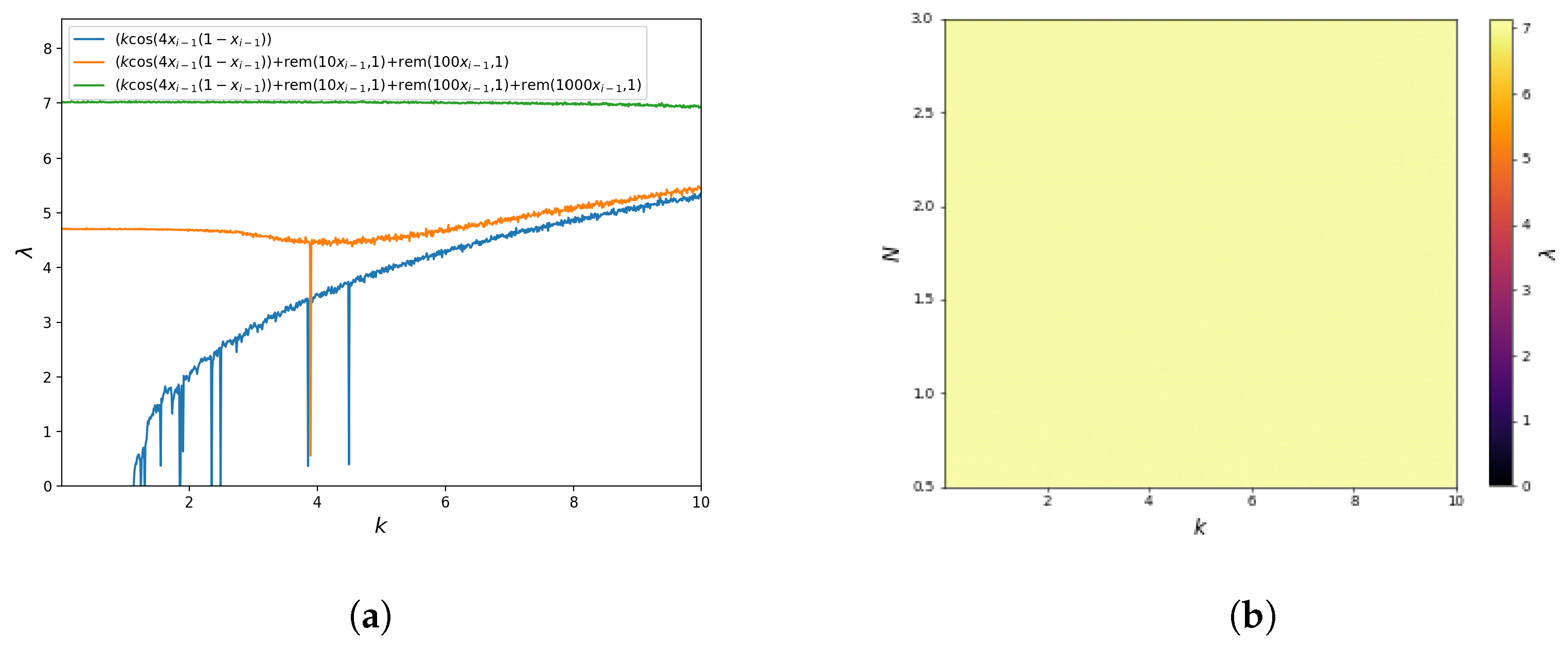
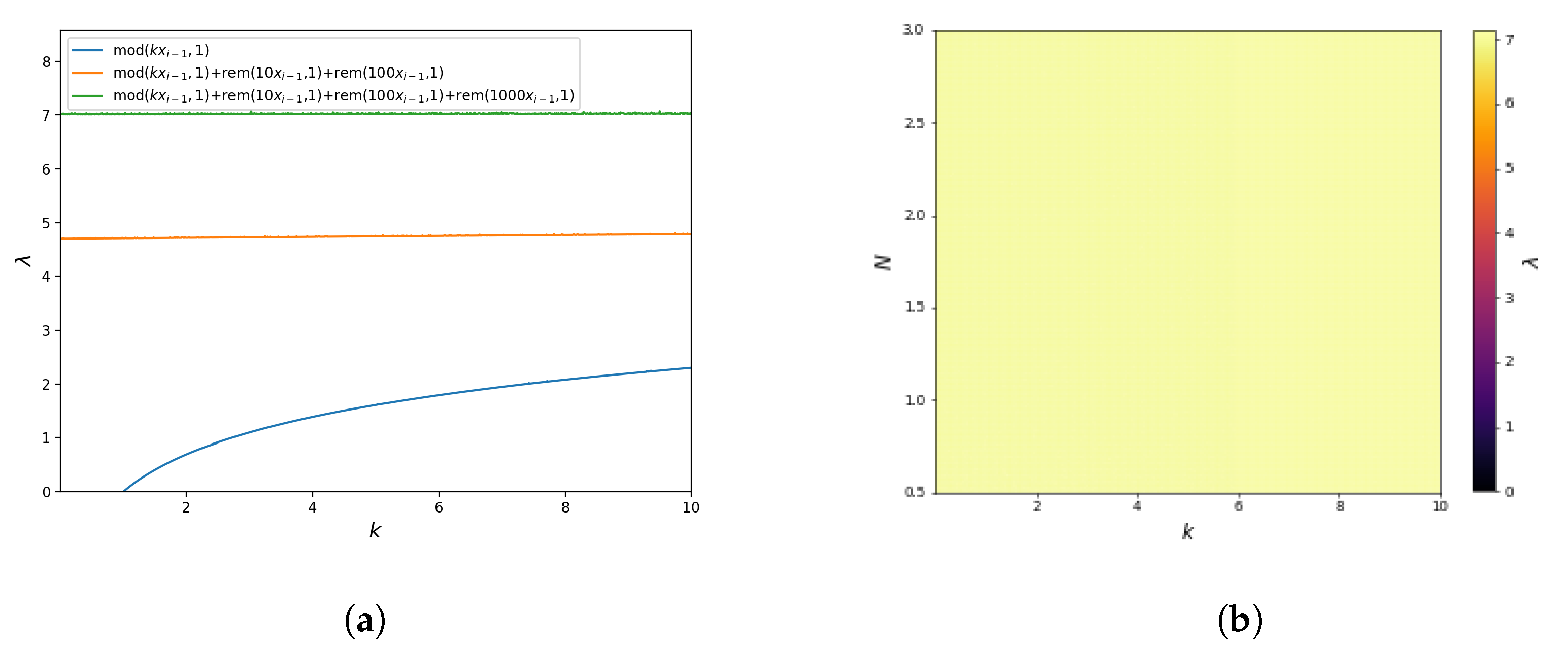
The map ${\mathcal{H}}_m\left(x_i\right)$ has a higher Lyapunov exponent if

$$\left|\sum _{j=1}^m{a}_j\right|>2\underset{x_i\in {\mathbb{D}}_m}{sup}\left|\dot{\mathcal{F}}\left(x_i\right)\right|,$$

(4)

where ${\mathbb{D}}_m$ is the domain of $\mathcal{F}$.

2. 

Let ${\lambda }_{\mu }$ denote the Lyapunov exponent of (3). If $a_{m+1}$ is selected, so that

$$\left|a_{m+1}\right|>2\underset{x_i\in {\mathbb{D}}_m}{sup}\left|{\dot{\mathcal{H}}}_m\left(x_i\right)\right|,$$

(5)

then ${\left({\lambda }_{\mu }\right)}_{\mu \in \mathbb{N}}$ is increasing.

Proof. 

We begin by considering the derivative of the remainder operation, which is

$${\displaystyle \frac{d}{dx}}rem\left(a·x,N\right)=a$$

(6)

for almost all x. Using (6), the derivative of ${\mathcal{H}}_m\left(x_i\right)$ as in (3) for almost all $x_i$ is

$${\dot{\mathcal{H}}}_m\left(x_i\right)={\dot{\mathcal{F}}}_m\left(x_i\right)+\sum _{j=1}^m{a}_j.$$

(7)

Observe that ${\sum }_{j=1}^m{a}_j$ is independent of $x_i$, and thus, if we denote it as

$$\widetilde{A_m}:=\sum _{j=1}^m{a}_j,$$

(8)

then

$${\dot{\mathcal{H}}}_m\left(x_i\right)={\dot{\mathcal{F}}}_m\left(x_i\right)+\widetilde{A_m}$$

(9)

which is exactly the case studied in [18], from which the conclusion is that, selecting

$$\widetilde{A_m}>2\underset{x_i\in {\mathbb{D}}_m}{sup}\left|\dot{\mathcal{F}}\left(x_i\right)\right|$$

(10)

results in a system with a greater Lyapunov exponent. Hence, in our case, the terms $a_j$ must be chosen so that ${\displaystyle \sum _{j=1}^m}{a}_j>2{sup}_{x_i\in {\mathbb{D}}_m}\left|\dot{\mathcal{F}}\left(x_i\right)\right|.$ We can extend the proof in that work by observing that a selection of

$$\widetilde{A_m}<-2\underset{x_i\in {\mathbb{D}}_m}{sup}\left|\dot{\mathcal{F}}\left(x_i\right)\right|$$

(11)

yields the same result. Thus, combining (10) and (11) yields that, selecting

$$\left|\sum _{j=1}^m{a}_j\right|>2\underset{x_i\in {\mathbb{D}}_m}{sup}\left|\dot{\mathcal{F}}\left(x_i\right)\right|$$

(12)

results in a system that has a higher Lyapunov exponent than that of the original system.

Observe that, until this point, no specific assumption has been made for each of the coefficients $a_j$ individually, only for their sum.

Next, we are interested in determining conditions such that the sequence of Lyapunov exponents created by adding extra terms in (3) is increasing. First of all, we observe that for every $m\in \mathbb{N}$, the domains of $\mathcal{F}$ and ${\mathcal{H}}_m$ coincide. With that in mind, we can then write

$$\begin{array}{cc}\hfill {\mathcal{H}}_{m+1}\left(x_i\right)=& \mathcal{F}\left(x_i\right)+\sum _{j=1}^{m+1}rem(a_j{x}_i,N_j)\hfill \end{array}$$

(13)

$$\begin{array}{cc}\hfill & =\mathcal{F}\left(x_i\right)+\sum _{j=1}^{m}rem(a_j{x}_i,N_j)+rem(a_{m+1}{x}_i,N_{m+1})\hfill \end{array}$$

(14)

$$\begin{array}{cc}\hfill & ={\mathcal{H}}_m\left(x_i\right)+rem(a_{m+1}{x}_i,N_{m+1}).\hfill \end{array}$$

(15)

Combining (15) with the first part of the proof and the fact that the domains of $\mathcal{F}$ and $\mathcal{H}$ coincide yields that selecting $a_{m+1}$ as

$$\left|a_{m+1}\right|>2\underset{x_i\in {\mathbb{D}}_m}{sup}\left|{\dot{\mathcal{H}}}_m\left(x_i\right)\right|$$

(16)

guarantees that ${\lambda }_{m+1}>{\lambda }_m$ for any m, which concludes the proof. □

Remark 1. 

Note that the choice of the remainder operator is made over the more common modulo operator, as the remainder operator does not change the sign of its input. This results in a more uniform distribution of the map’s values, compared to the use of the modulo. Figure 2 illustrates this difference using a modified version of the Sine Map. In addition, it is worth noting that the remainder operator results in a symmetric distribution in this case. In contrast, the map distribution with the modulo operator does not have such symmetry.

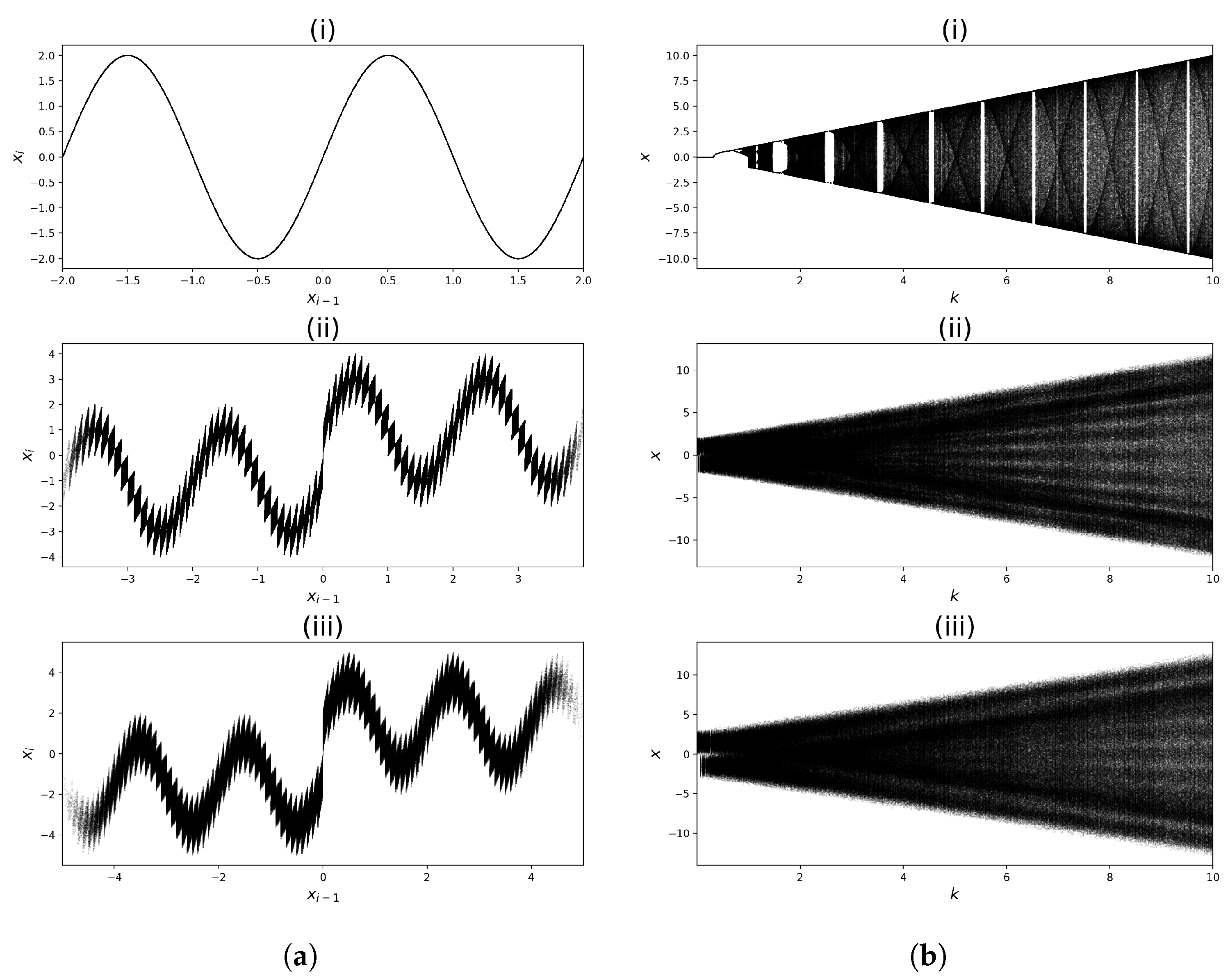
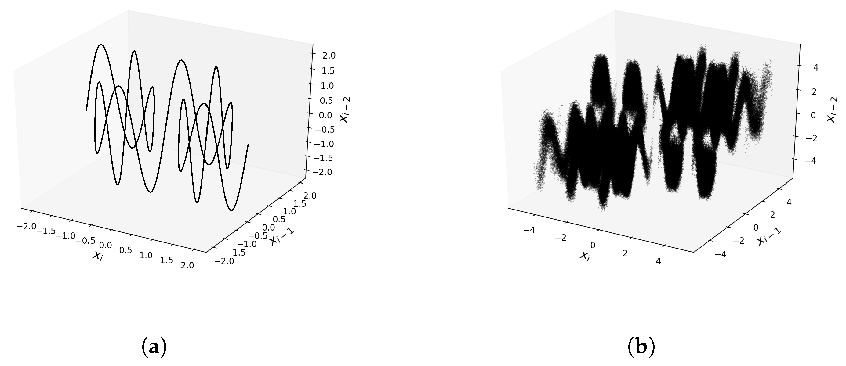
3. Chaotification Examples for Different Chaotic Maps

In this section, we apply the above chaotification technique to several well-known maps as shown below.

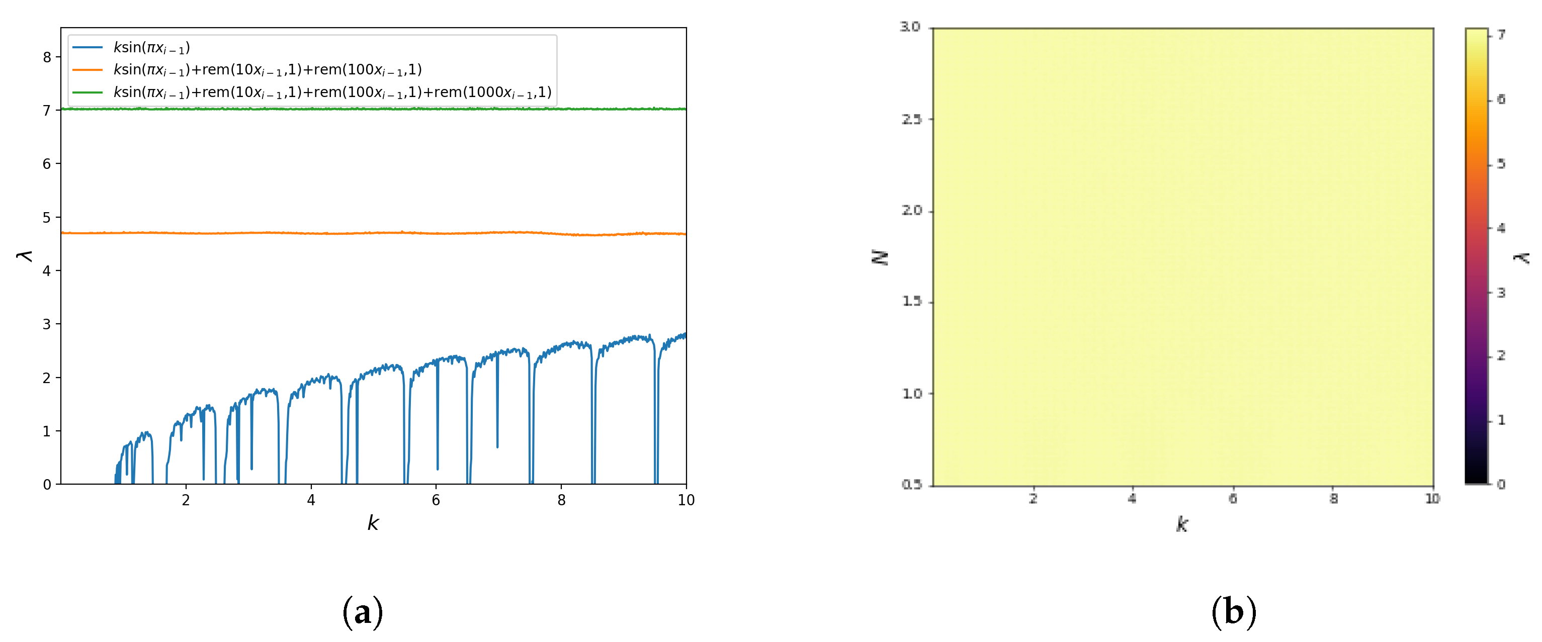
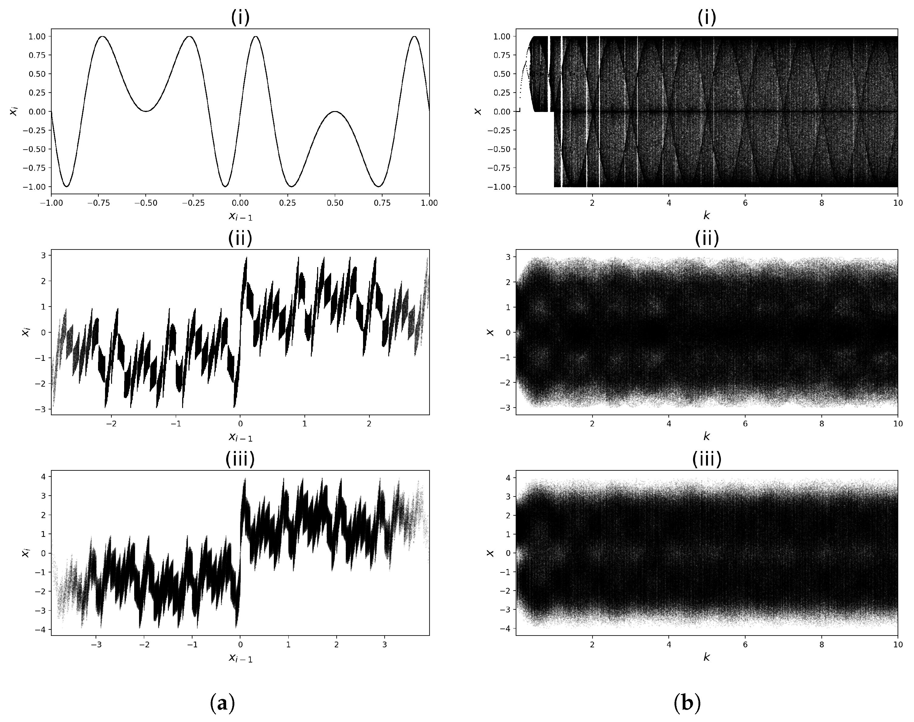
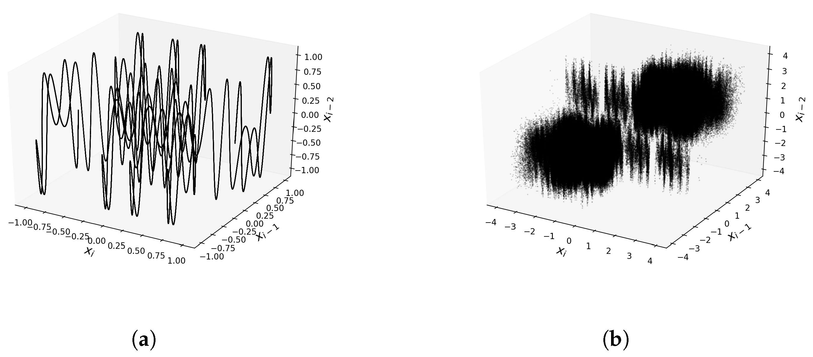
3.1. Sine Map

Consider the well-known Sine Map [37,38]:

$$x_i=ksin\left(\pi x_{i-1}\right).$$

(17)

Using the Sine Map (17) as the base function $\mathcal{F}\left(x\right)$, two cases of mappings of the form (2) are further analysed, for $m=2$ and $m=3$:

$$x_i=ksin\left(\pi x_{i-1}\right)+rem(10x_{i-1},1)+rem(100x_{i-1},1),$$

(18)

$$x_i=ksin\left(\pi x_{i-1}\right)+rem(10x_{i-1},1)+rem(100x_{i-1},1)+rem(1000x_{i-1},1).$$

(19)

The first map (18), apart from the base function (17), consists of two additional components: $rem(10x_{i-1},1)$ and $rem(100x_{i-1},1)$. In turn, the second map (19) modifies the first with an additional component: $rem(1000x_{i-1},1)$.

One of the tools for analysing dynamical systems is to present the so-called phase diagrams that show the system’s relationship $(x_{i-1},x_i)$. The phase diagrams of all three cases (Sine Map (17) and its two modifications (18) and (19)) for fixed parameter values are presented in Figure 3a. These graphs show that adding multiple $rem(·)$ operators causes a significant increase in the complexity of the base mapping. In turn, Figure 3b presents bifurcation diagrams of the analysed mappings. This figure depicts the existence of the so-called periodic windows for the Sine Map (17) and their respective absence for the modified mappings (18) and (19). This means that, in the case of mappings (18) and (19), there is no worry about choosing the proper mapping parameters, as any choice will always result in chaotic behaviour.

The increased complexity of the resulting maps is also confirmed by the three-dimensional phase diagrams, which show the relation of points $(x_i,x_{i-1},x_{i-2})$. These charts are presented in Figure 4. In the case of the Sine Map (17), the graph in Figure 4a shows that points fall on a curve, while for the modified maps (19) (Figure 4b), they fill up a 3D region, forming a cloud of points. Therefore, the mapping with the $rem(·)$ operators is much more complex than the base mapping.

Chaotic systems are characterised by the system’s sensitivity to a change in initial conditions, which is measured using the Lyapunov exponent $\lambda$ given by the formula:

$$\lambda =\underset{n\to \infty }{lim}\frac{1}{n}\sum _{i=0}^{n-1}ln\left|{\mathcal{F}}^{\prime }\left(x_i\right)\right|.$$

(20)

The plot of the Lyapunov exponent is shown in Figure 5a. This figure clearly shows the presence of stable/periodic regions for the Sine Map (17) and their absence for mappings with the $rem(·)$ operator. This figure also shows that the sensitivity to the change of initial conditions for the mappings (18) and (19) is roughly constant for the entire range of the parameter k. Thus, after the same number of iterations, the system will lose information about the initial conditions.

Moreover, to better illustrate the chaotic nature of the analysed dynamical systems, the Lyapunov exponent value $\lambda$’s dependence on $(k,N)$ is calculated. The results are shown in Figure 5b. The obtained values show that $\lambda >0$ for the entire analysed parameter range for the mapping (19). Moreover, the $\lambda$ value is roughly constant for the whole range of parameter values. These results are consistent with the value of the Lyapunov exponent from Figure 5a. They also confirm that the mapping (19) is characterised by interrupted chaotic behaviour for large ranges of parameter changes and, thus, has a much more complex behaviour than the base function Sine Map (17).

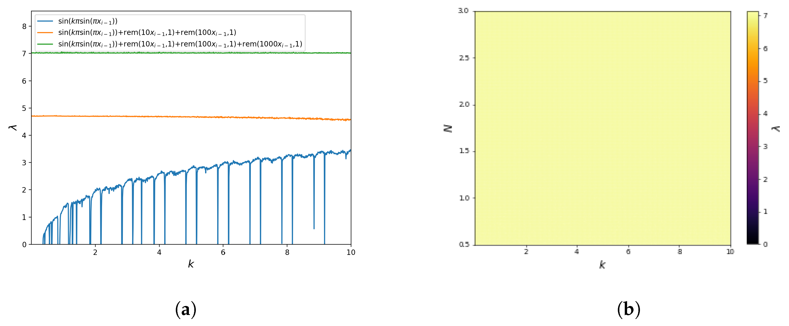
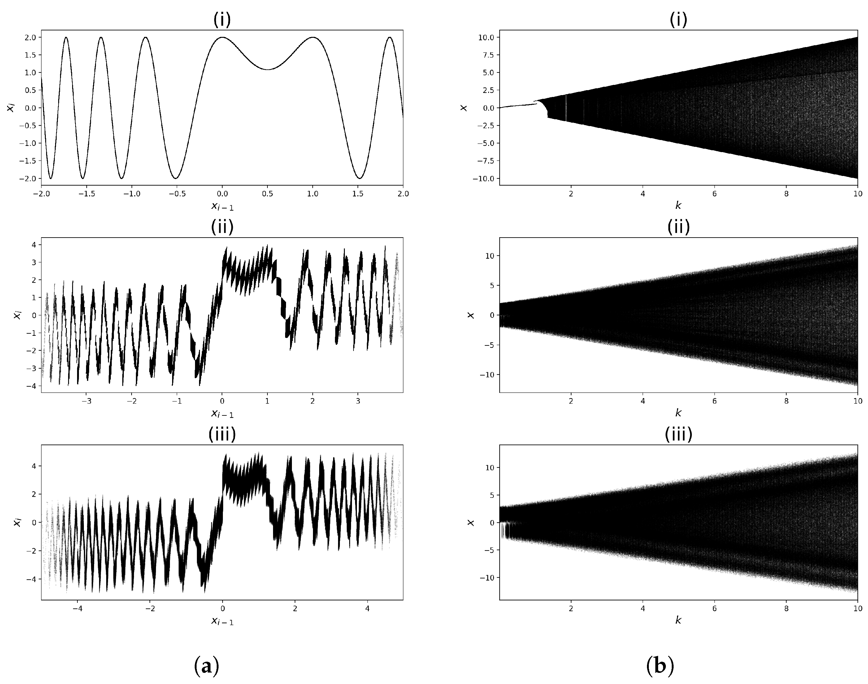
3.2. Sine-Sine Map

In [6] a sine chaotification was proposed. As an example of this method, consider the Sine-Sine Map:

$$x_i=sin(\pi ksin\left(\pi x_{i-1}\right)).$$

(21)

As in the case of the Sine Map (17), the Sine-Sine Map (21) was also used as the base function $\mathcal{F}\left(x\right)$, and two new maps are defined, which will be analysed further in the paper:

$$x_i=sin(\pi ksin\left(\pi x_{i-1}\right))+rem(10x_{i-1},1)+rem(100x_{i-1},1),$$

(22)

$$x_i=sin(\pi ksin\left(\pi x_{i-1}\right))+rem(10x_{i-1},1)+rem(100x_{i-1},1)+rem(1000x_{i-1},1).$$

(23)

Their design is very similar to the previous case, i.e., the first one, apart from the base function having two additional components $rem(10x_{i-1},1)$ and $rem(100x_{i-1},1)$. In turn, the second one has one more component equal to $rem(1000x_{i-1},1)$.

As previously, the phase diagrams of all three cases (Sine–-Sine Map (21) and its two modified versions (22) and (23)) for various fixed parameter values are presented in Figure 6a. These graphs confirm that adding multiple $rem(·)$ operators causes a significant increase in the complexity of the base mapping. In addition, Figure 6b presents bifurcation diagrams of the analysed mappings. This figure also demonstrates that, although there are visible periodic windows for the Sine-Sine Map (21), they are absent for the modified mappings (22) and (23). Similar to the Sine Map, this means that any choice of mapping parameters in (22) or (23) will always result in chaotic behaviour.

The three-dimensional phase diagram confirms the increase of complexity also in this case. These relevant plots are presented in Figure 7. In the case of the Sine–-Sine Map (21), the graph in Figure 7a consists of points forming a curve, while for the map (23) (Figure 7b), points fill up a 3D region indicating that the mapping with the $rem(·)$ operators is much more complex than the base mapping.

Similar to the sine map analysis, the Lyapunov exponent was also calculated, showing the significant increase of the system’s sensitivity to initial conditions after the chaotification is applied. The plot of the Lyapunov exponent is shown in Figure 8a. The results are very similar to the Sine Map case. This figure clearly shows the presence of stable regions for the Sine–-Sine Map (21) and their absence for mappings with the $rem(·)$ operator. This figure also shows that the sensitivity to the change of initial conditions for the mappings (22) and (23) is roughly constant for the entire range of the parameter k. Thus, after the same number of iterations, the system will lose information about the initial conditions.

Moreover, for these mappings, the Lyapunov exponent value $\lambda$ was also determined as a function of parameters $(k,N)$. The results are shown in Figure 8b. The obtained values show that $\lambda >0$ for the entire analysed parameter range for the mapping (23). Moreover, $\lambda$ is roughly constant for the whole range of parameter values. These results are consistent with the value of the Lyapunov exponent from Figure 8a. The obtained results confirmed that the mapping (23) is characterised by interrupted chaotic behaviour for large ranges of parameter changes and, therefore, has a much more complex behaviour than the base function Sine–Sine Map (21).

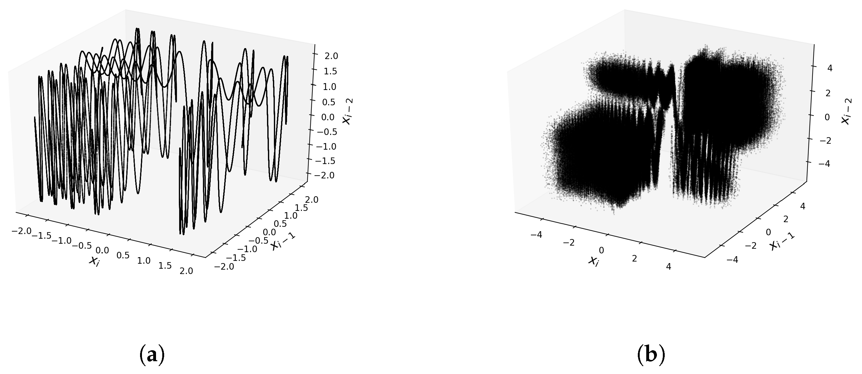
3.3. Cosine–Logistic Map

In [5] a cosine chaotification was proposed. As an example of this method, consider the Cosine–-Logistic Map:

$$x_i=kcos\left(r{x}_{i-1}(1-x_{i-1})\right).$$

(24)

As in the case of the analysed previous maps, the Cosine–-Logistic Map (24) was also used as the base function $\mathcal{F}\left(x\right)$, and two new maps are defined, which will be analysed further in the paper:

$$x_i=kcos\left(4x_{i-1}(1-x_{i-1})\right)+rem(10x_{i-1},1)+rem(100x_{i-1},1),$$

(25)

$$x_i=kcos\left(4x_{i-1}(1-x_{i-1})\right)+rem(10x_{i-1},1)+rem(100x_{i-1},1)+rem(1000x_{i-1},1).$$

(26)

Their design is very similar to the previous cases, i.e., the first one, apart from the base function, has two additional components $rem(10x_{i-1},1)$ and $rem(100x_{i-1},1)$. In turn, the second one has one more component equal to $rem(1000x_{i-1},1)$.

As before, phase diagrams of all three cases (the base Cosine–Logistic Map (24) and its two modifications (25) and (26))) for fixed parameter values are presented in Figure 9a. These graphs confirm that adding multiple $rem(·)$ operators causes a significant increase in the complexity of the base mapping. Figure 9b presents bifurcation diagrams of the analysed mappings. This figure shows that the behaviour of the Cosine–Logistic Map (24) is more complex than the behaviour of the previous base functions, i.e., after some value of the k parameter, there are no visible periodic windows. However, the mappings (25) and (26) also do not have visible periodic windows. Similar to the previous cases, this means that the choice of the mapping parameters in (25) or (26) will always result in chaotic behaviour.

Figure 10a,b also depict the difference between the three-dimensional phase diagrams of the Cosine–Logistic Map (24) and the map (26). The original map has a curve diagram, but the modified map fills a wide 3D region.

The respective plots of the Lyapunov exponent are shown in Figure 11a. The results are very similar to the Sine–-Sine Map. This figure clearly shows the presence of stable regions for the Cosine–Logistic Map (24) and their absence for the respective modified mappings with the $rem(·)$ operator. This figure also shows that the sensitivity to the change of initial conditions for the mappings (25) and (26) is roughly constant for the entire range of the parameter k. Thus, after the same number of iterations, the system will lose information about the initial conditions.

Moreover, for these mappings, the Lyapunov exponent value $\lambda$ was determined as a function of $(k,N)$. The results are shown in Figure 11b. The obtained values show that $\lambda >0$ for the entire analysed parameter range for the mapping (26). Moreover, the $\lambda$ value is roughly constant for the whole range of parameter values. These results are consistent with the value of the Lyapunov exponent from Figure 11a. Again, the obtained results confirm that the mapping (26) is characterised by interrupted chaotic behaviour for large ranges of parameter changes and, thus, has a much more complex behaviour than the base function Cosine–Logistic Map (24).

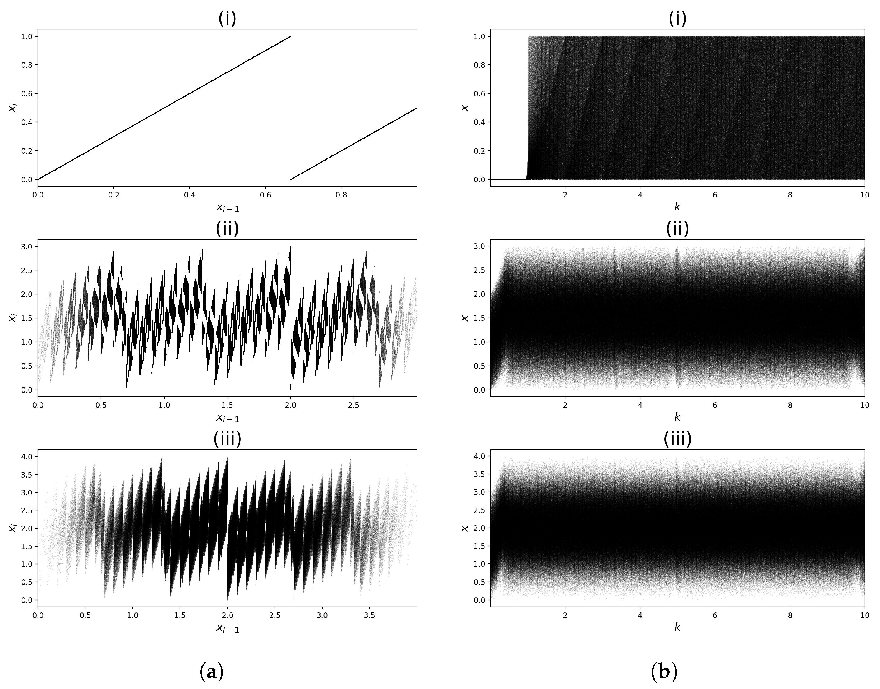
3.4. Renyi Map

Consider the Renyi Map [39]:

$$x_i=\mathrm{mod}(k{x}_{i-1},1).$$

(27)

Finally, the Renyi Map (27) was also used as the base function $\mathcal{F}\left(x\right)$, and two new maps are defined, which will be analysed further in the paper:

$$x_i=\mathrm{mod}(k{x}_{i-1},1)+rem(10x_{i-1},1)+rem(100x_{i-1},1),$$

(28)

$$x_i=\mathrm{mod}(k{x}_{i-1},1)+rem(10x_{i-1},1)+rem(100x_{i-1},1)+rem(1000x_{i-1},1).$$

(29)

The design is very similar to the previous cases, i.e., the first one, apart from the base function, has two additional components $rem(10x_{i-1},1)$ and $rem(100x_{i-1},1)$. In turn, the second one has one more component equal to $rem(1000x_{i-1},1)$.

As in the earlier analysis, the phase diagrams of all three cases (Renyi Map (27) and its two modifications (28) and (29)) for fixed parameter values are presented in Figure 12a. These graphs confirm that adding multiple $rem(·)$ operators causes a significant complication in the base mapping. In turn, Figure 12b presents bifurcation diagrams of the analysed mappings. This figure shows that the behaviour of the Renyi Map (27) is also very complicated, with no visible periodic windows (the stable states occur in this map for $k\in \mathbb{N}$). However, the mappings (28) and (29) also do not have visible periodic windows. As in the previous cases, this situation means that choosing the mapping parameters in (28) or (29) will always result in a chaotic behaviour of the system.

The three-dimensional phase diagrams are shown in Figure 13 for the Renyi Map (27) and the map (29). The Renyi Map diagram consists of piecewise linear parts, while the modified map has a phase diagram that is more dense and covers a 3D area.

Similar to the analysis of the previous maps, plots of the Lyapunov exponent were also determined in this case, showing the system’s sensitivity to the change of the initial conditions. The plot of the Lyapunov exponent is shown in Figure 14a. The obtained results are very similar to the previous case. This figure clearly shows the presence of stable regions for the Renyi Map (27) and their absence for mappings with the $rem(·)$ operator. This figure also shows that the sensitivity to the change of initial conditions for the mappings (28) and (29) is roughly constant for the entire range of the parameter k. Thus, after the same number of iterations, the system will lose information about the initial conditions.

Again, the Lyapunov exponent value $\lambda$ was also determined with respect to $(k,N)$. The results are shown in Figure 14b. The obtained values show that $\lambda >0$ for the entire analysed parameter range for the mapping (29). Moreover, $\lambda$ is roughly constant for the whole range of parameter values. These results are consistent with the value of the Lyapunov exponent from Figure 14a. The obtained results confirm that the mapping (29) is characterised by interrupted chaotic behaviour for large ranges of parameter changes and, thus, has a much more complex behaviour than the base function Renyi Map (27).

4. Effect on Key Space

Let $\mathcal{K}$ denote the key space of a seed map, that is the sum of all possible key parameter combinations for that map, which can result in unique solution trajectories. The proposed chaotification technique (2) introduces $2m$ additional parameters, $a_j,N_j$, $j=1,\dots ,m$. Assuming a D digit accuracy, this results in a multiplicative increase of the key space by ${10}^{2mD}$. If we let $D=16$, the key space increase is ${10}^{32m}\approx {\left({10}^3\right)}^{10.6m}\approx {\left(2^{10}\right)}^{10.6m}=2^{106m}$. In the proposed examples, there are three added terms, so $m=3$, and the increase is approximately $2^{318}$.

Table 1. Key space of the considered maps.

Chaotic System
	Sine (17)	Sine–Sine (21)	Cosine–Logistic (24)	Renyi (27)
Seed	$2^{53}$	$2^{53}$	$2^{106}$	$2^{53}$
Modified	$2^{373}$	$2^{373}$	$2^{426}$	$2^{373}$

lists the key spaces for all the considered maps.

5. Operations per Iteration

Here, the number of operations that the technique introduces in a single iteration is counted. The results are summarised in

Table 2. Number of operations per iteration for the modified maps.

		Chaotic System
Operation	(2) ($m=3$)	Mod. Sine (19)	Mod. Sine–Sine (23)	Mod. Cos.–Logistic (26)	Mod. Renyi (29)
Addition	m (3)	3	3	4	3
Multiplication	m (3)	5	5	6	4
Sinusoidal	0	1	2	1	0
Remainder	m (3)	3	3	3	4
Overall	3m (9)	12	13	14	11

. For m remainder terms, the chaotification technique requires 3 m additional operations, so the computational complexity of the chaotification technique increases linearly with the number of remainder operators.

Note that, in Table 2, operations that can be precomputed only once are not counted. For example, the term $\pi k$ in the Sine–-Sine Map (21) only needs to be computed once and not repeated in every iteration.

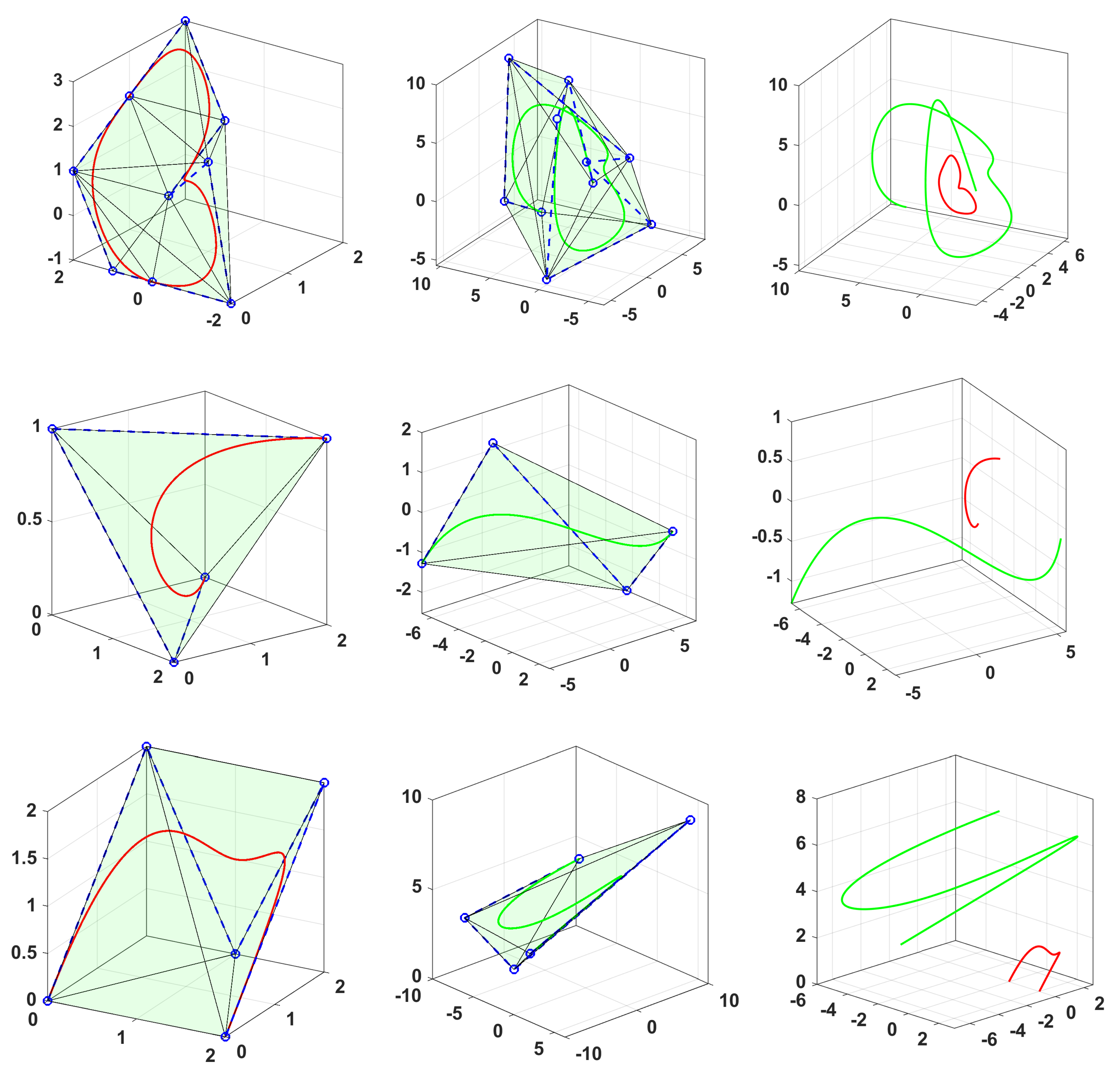
6. Application to Symmetric Encryption of B-Spline Curves

6.1. B-Spline Basics

A B-spline curve of degree n is characterised by its control points. Given $p+1$ control points $P_i\in {\mathbb{R}}^d$ in the d-dimensional space, the curve is described by

$$x\left(t\right)=\sum _{i=0}^p{N}_i^n\left(t\right)P_i,$$

(30)

where $N_i^n\left(t\right)$ are the B-spline basis polynomials of degree n. The curve is defined over a knot sequence T in the interval $t\in [0,1]$, which we assumed here as uniform, described by

$$T=[t_0,\dots ,t_{p+n+1}]=\left[\underset{n+1}{\underbrace{0,\dots ,0}},t_{n+1},\dots ,t_p,\underset{n+1}{\underbrace{1,\dots ,1}}\right].$$

(31)

The repetition of the first and last knots is performed so that the curve interpolates the first and last control points and is also tangent to the control polygon.

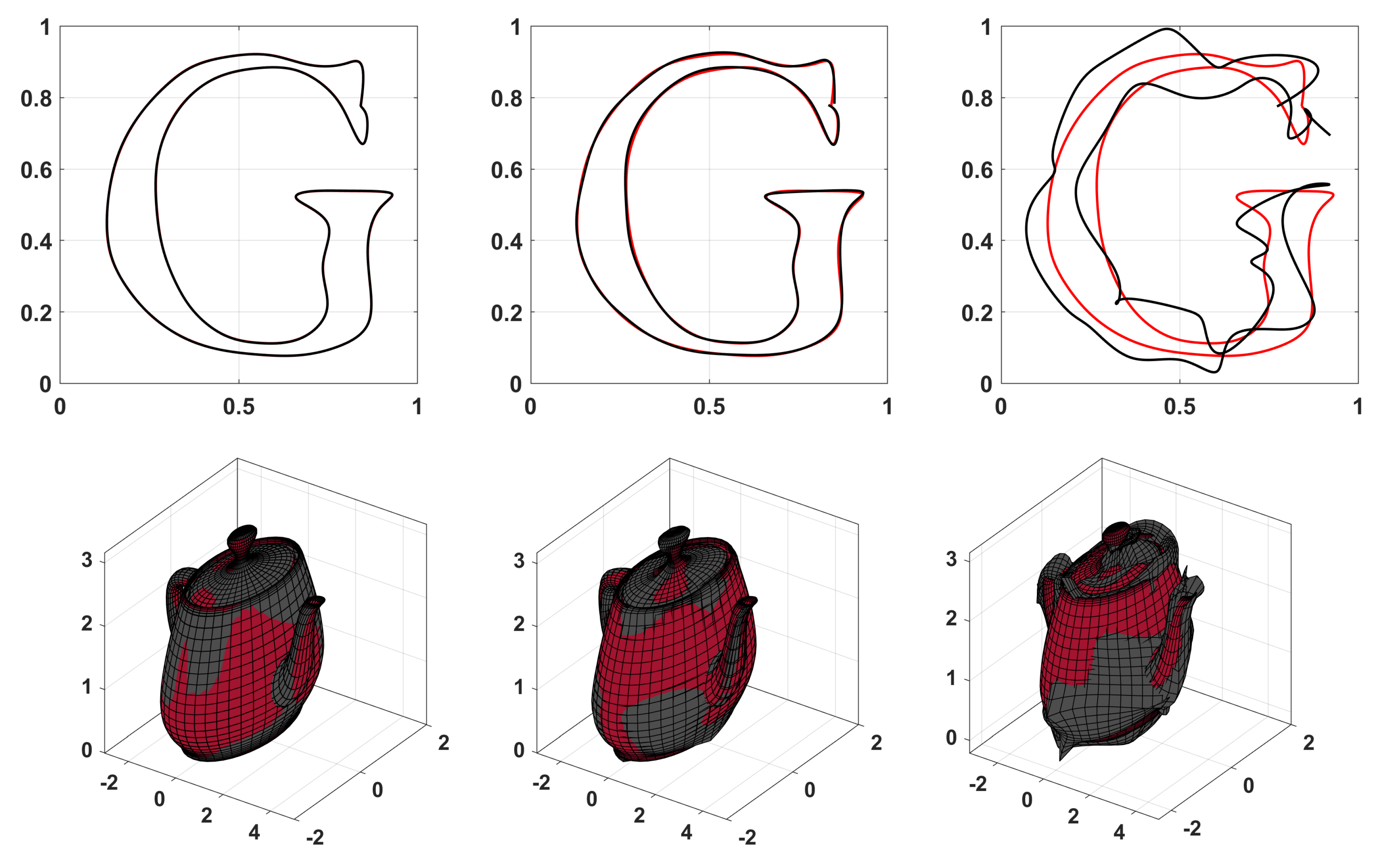
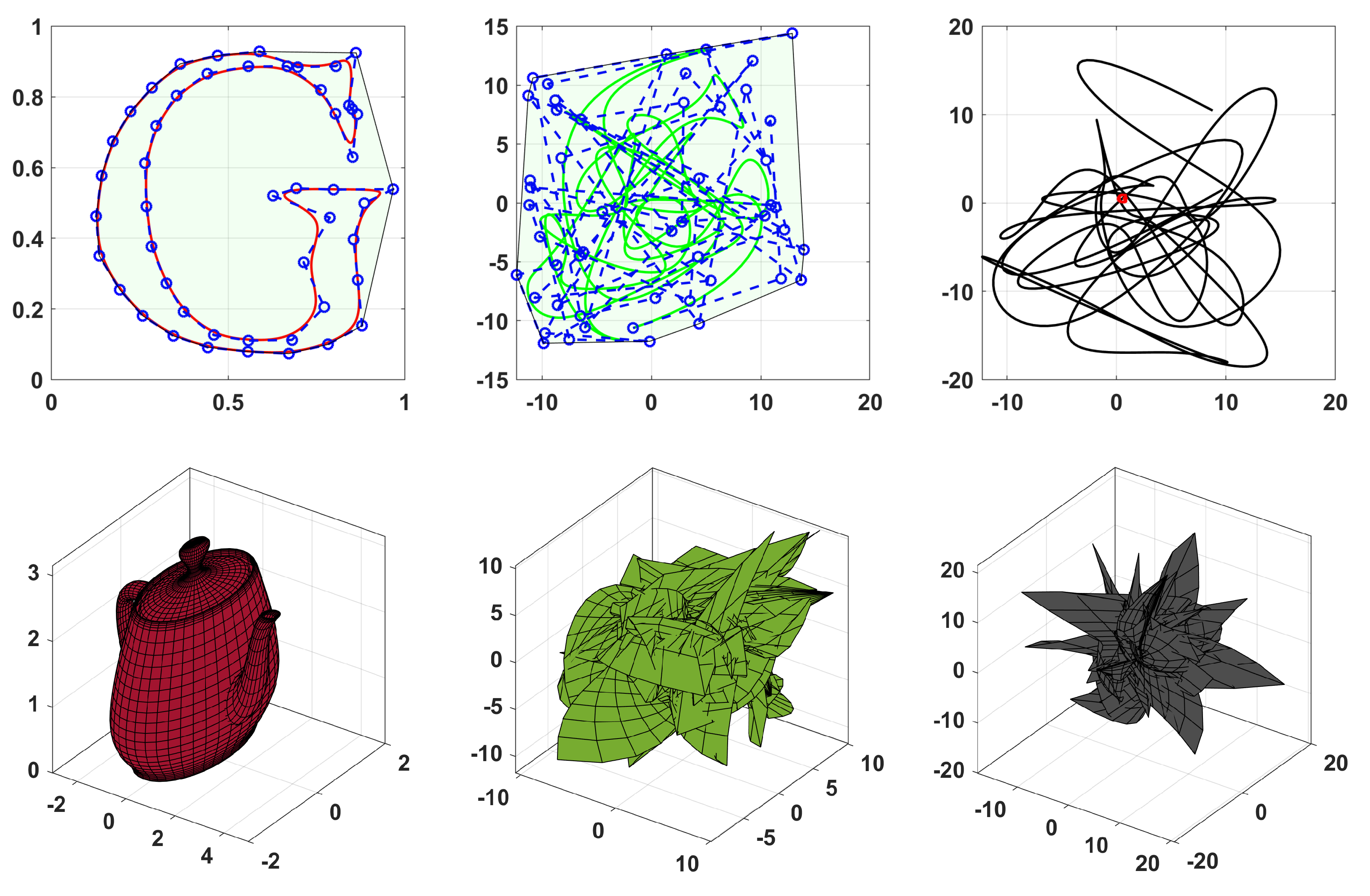
6.2. Encryption of a B-Spline Curve

As described in the previous section, the information required to completely describe a B-Spline curve is its control points $P_0,\dots ,P_p$ arranged in order, the polynomial degree n, and a knot sequence. Thus, the encryption of a curve should aim at masking these characteristics. As changing the polynomial order would effect the proper definition of the knot sequence, here we assumed that the encryption process will not affect the degree of the curve. The same holds for the knot sequence. The proposed encryption will not affect it, as it is fairly common to assume a uniform knot sequence. If required though, an optional step can be added, encrypting the knot sequence as well.

The procedure is described in the steps below. There are two main steps involved: a shuffling of the plaintext values and a modulation through addition. The purpose of the shuffling step is to disperse the information regarding the sequence of control points, for all their coordinates. The second step hides this information, by combining it with the values of a chaotic map. For both steps, a chaotic map is used, chosen from the ones presented in the previous section. Here, the modified Sine Map (19) is considered as an example.

Here, it is worth noting that a common, and very effective substitution action is the exclusive or (XOR) operation, which is performed on the binary level of the plaintext. Here, since the plaintext consists of rational numbers, the application of the XOR operation is possible only after transforming to binary format, for example using the IEEE-754 standard. However, as this is deemed time-consuming, the more computationally efficient option of additive modulation was chosen:

Input. 

A plaintext B-spline curve described by its control points $P_0,\dots ,P_p\in {\mathbb{R}}^d$ arranged in a matrix $\mathsf{\Pi }=(P_0,\dots ,P_p)\in {\mathbb{R}}^{d\times (p+1)}$, the polynomial degree n, and a knot sequence U. It is assumed that all the control point coordinates lie in the interval $[-B,B]$.

A chaotic map of the form (19), with key parameters $k,a_1,a_2,a_3,N_1,N_2,N_3$, to be computed below.

Data setup. 

First, the entries of $\mathsf{\Pi }$ are concatenated in a single vector ${\mathsf{\Pi }}_{row}$ of size $1\times d·(p+1)$ as follows:

$${\mathsf{\Pi }}_{row}=\left(\begin{array}{ccccccc}{P}_{0,1}& P_{0,2}& \cdots P_{0,d}& \cdots P_{1,1}& \cdots P_{1,d}& \cdots & P_{p,d}\end{array}\right)$$

(32)

where $P_{i,j}$ represents the j-th coordinate of the $P_i$ control point.

Key setup. 

To make the design resistant to plaintext attacks, the map keys should be plaintext-dependent. This achieves the confusion task in encryption. They are initialised as

$$\begin{array}{ccc}\hfill x_0& =& mean\left({\mathsf{\Pi }}_{row}\right)/\left|\right|{\mathsf{\Pi }}_{row}\left|\right|\hfill \end{array}$$

(33)

$$\begin{array}{ccc}\hfill k& =& B+\mathrm{entropy}\left({\mathsf{\Pi }}_{row}\right)\hfill \end{array}$$

(34)

$$\begin{array}{ccc}\hfill a_1& =& 10+\mathrm{mean}\left({\mathsf{\Pi }}_{row}\right)\hfill \end{array}$$

(35)

$$\begin{array}{ccc}\hfill a_2& =& 100+\mathrm{var}\left({\mathsf{\Pi }}_{row}\right)\hfill \end{array}$$

(36)

$$\begin{array}{ccc}\hfill a_3& =& 1000\hfill \end{array}$$

(37)

$$\begin{array}{ccc}\hfill N_1& =& 1\hfill \end{array}$$

(38)

$$\begin{array}{ccc}\hfill N_2& =& 1\hfill \end{array}$$

(39)

$$\begin{array}{ccc}\hfill N_3& =& 1\hfill \end{array}$$

(40)

where $\left|\right|·\left|\right|$ denotes the Euclidean norm.

Step 1. 

The first step is to shuffle the sequence of the control points. This is also part of the usual confusion step in encryption, which disperses the plaintext information. For the shuffling operation, the following pseudo-random number generator (PRNG) is utilised:

$$p_i=\lfloor \mathrm{mod}({10}^8{x}_i,d·(p+1))\rfloor +1,$$

(41)

which generates integers in the interval $[1,d·(p+1)]$, until $d·(p+1)$ discrete values are generated. If an integer is generated twice, it is discarded the second time. The result is a list of $d·(p+1)$ non-repeating integers, denoted as $S=(s_0,\dots ,s_{d·(p+1)-1})$. These integers represent the new order of the elements of the vector ${\mathsf{\Pi }}_{row}$. Therefore, the $s_0$ element of ${\mathsf{\Pi }}_{row}$ is moved to the first position, the $s_1$ element of ${\mathsf{\Pi }}_{row}$ is moved to the second position, and so on. The resulting matrix, which contains the re-arranged elements of ${\mathsf{\Pi }}_{row}$, is denoted as ${\mathsf{\Sigma }}_{row}$:

$${\mathsf{\Sigma }}_{row}=\left(\begin{array}{cccc}{\mathsf{\Sigma }}_{row,0}& {\mathsf{\Sigma }}_{row,1}& \cdots & {\mathsf{\Sigma }}_{row,d·(p+1)-1}\end{array}\right)$$

(42)

Step 2. 

The next step is the diffusion of the shuffled plaintext. The values of the vector ${\mathsf{\Sigma }}_{row}$ are masked using the values of the chaotic map used in Step 1. Continuing the iteration of the map from Step 2 (without making use of the PRNG), the elements of ${\mathsf{\Sigma }}_{row}$ are masked as follows:

$$\begin{array}{ccc}\hfill C_0& =& {\mathsf{\Sigma }}_{row,0}+x_i\hfill \end{array}$$

(43)

$$\begin{array}{ccc}\hfill C_1& =& {\mathsf{\Sigma }}_{row,1}+x_{i+1}\hfill \\ & ⋮& \hfill \end{array}$$

(44)

$$\begin{array}{ccc}\hfill C_{d·(p+1)-1}& =& {\mathsf{\Sigma }}_{row,d·(p+1)-1}+x_{i+d·(p+1)-1}\hfill \end{array}$$

(45)

where the i index in $x_i$ is used to denote that the map is being iterated, continuing from the previous Step 1. The resulting values are arranged in a vector:

$${\mathsf{\Psi }}_{row}=\left(\begin{array}{cccc}{C}_0& C_1& \cdots & C_{d·(p+1)-1}\end{array}\right)$$

(46)

Step 3. 

After the substitution step is finished, the elements of ${\mathsf{\Psi }}_{row}$ are reshaped into an $d\times (p+1)$ matrix $\mathsf{\Psi }=(E_0,\dots ,E_p)$, where each column represents a ciphertext control point, similar to the matrix $\mathsf{\Pi }$.

Output. 

A ciphertext B-spline curve described by its control points $E_0,\dots ,E_p$, the polynomial degree n, and a knot sequence U.

6.3. Decryption Process

The decryption process follows the exact same steps, in reverse order. These are described below:

Input. 

A ciphertext B-spline curve described by its control points $E_0,\dots ,E_p$, the polynomial degree n, and a knot sequence U.

A chaotic map of the form (19), with key parameters $k,a_1,a_2,a_3,N_1,N_2,N_3$.

Step 1. 

The first step is to arrange the elements of the ciphertext control points $E_0,\dots ,E_p$ in a $1\times d·(p+1)$ vector, as Equation (46).

Step 2. 

The PRNG (41) is initialised. The PRNG generates integers in the interval $[1,d·(p+1\left)\right]$, until $d·(p+1)$ discrete values are generated. Therefore, if an integer is generated twice, it is discarded the second time. The result is a list of $d·(p+1)$ non-repeating integers, denoted as $S=(s_0,\dots ,s_{d·(p+1)-1})$.

After this process is finished, the map is iterated again $d\times (p+1)$ times, to generate the values $x_i,\dots ,x_{i+d·(p+1)-1}$. The i index here denotes that the map is iterated consecutively from the previous process of generating S.

Step 3. 

The confusion is reversed as

$$\begin{array}{ccc}\hfill {\mathsf{\Sigma }}_{row,0}& =& C_0-x_i\hfill \end{array}$$

(47)

$$\begin{array}{ccc}\hfill {\mathsf{\Sigma }}_{row,1}& =& C_1-x_{i+1}\hfill \\ & ⋮& \hfill \end{array}$$

(48)

$$\begin{array}{ccc}\hfill {\mathsf{\Sigma }}_{row,d·(p+1)-1}& =& C_{d·(p+1)-1}-x_{i+d·(p+1)-1}\hfill \end{array}$$

(49)

The resulting elements are combined in a vector as Equation (42).

Step 4. 

The next step is to reverse the shuffling of the elements of ${\mathsf{\Sigma }}_{row}$.

The elements of S from Step 2 indicate the shuffling that was originally performed in the encryption process. The procedure is reversed, by moving the first element into the $s_0$ position, the second element into the $s_1$ position, and so on, until the last element is moved into the $s_{d·(p+1)-1}$ position. The new matrix is denoted as ${\mathsf{\Pi }}_{row}$.

Step 5. 

Finally, the elements of ${\mathsf{\Pi }}_{row}$ are reshaped into an $m\times (p+1)$ matrix $\mathsf{\Pi }=(P_0,\dots ,P_p)$, where each column represents the plaintext control point.

Output. 

A plaintext B-spline curve described by its control points $P_0,\dots ,P_p\in {\mathbb{R}}^d$ arranged in a matrix $\mathsf{\Pi }=(P_0,\dots ,P_p)\in {\mathbb{R}}^{d\times (p+1)}$, the polynomial degree n, and a knot sequence U.

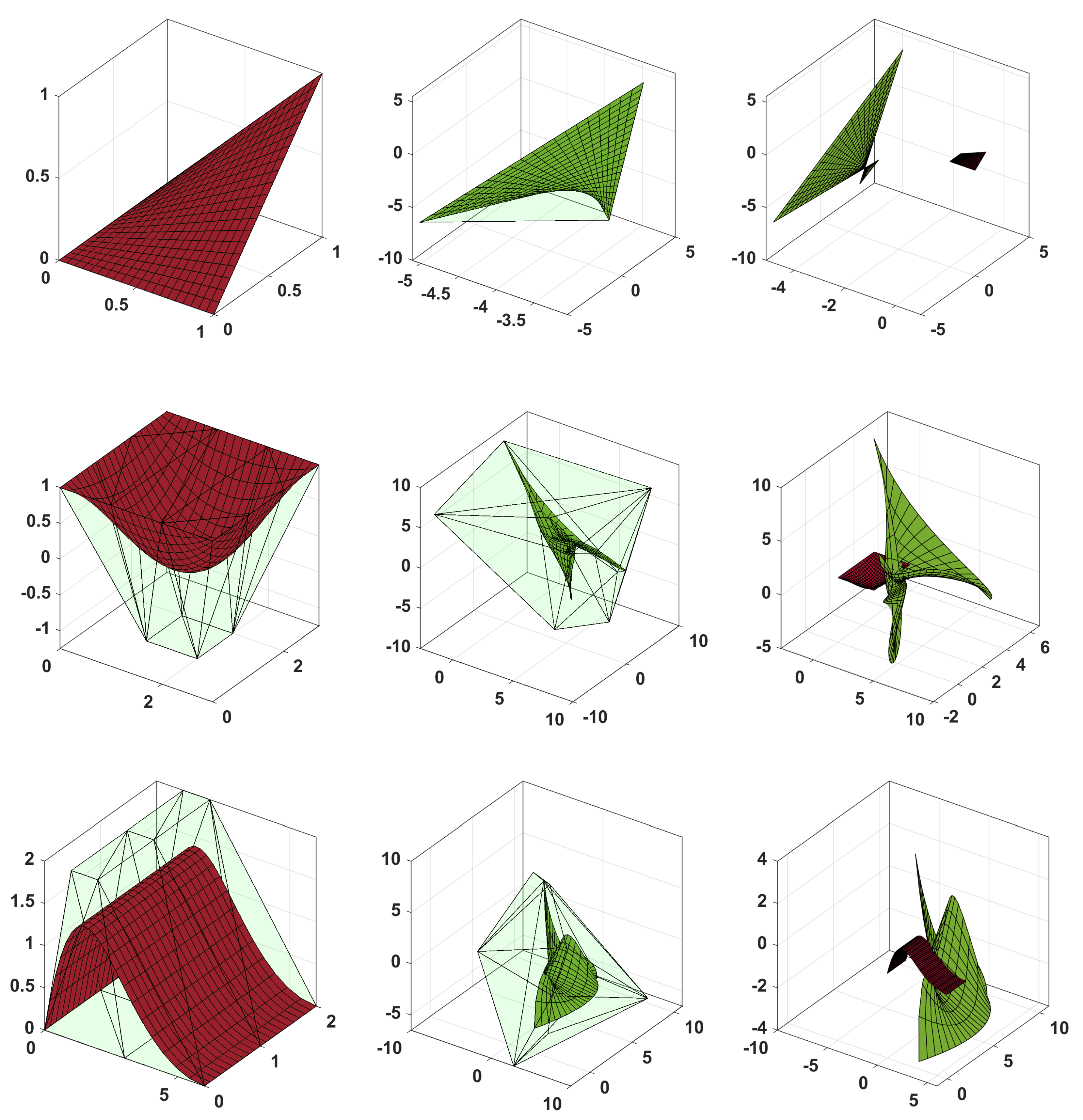
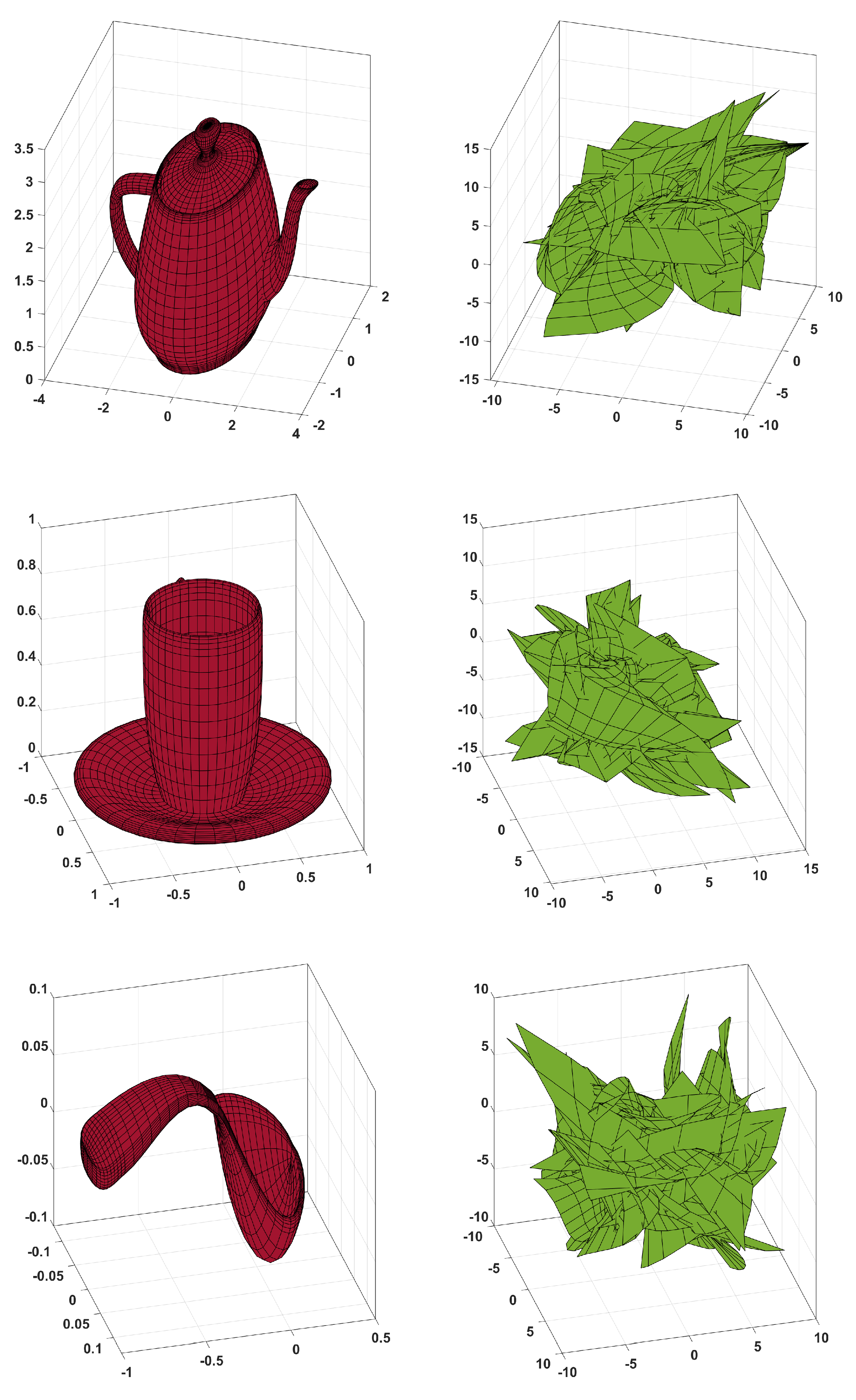
7. Patch Encryption

B-spline patches are obtained by considering a net of control points $P_{i,j}\in {\mathbb{R}}^3$, $i=0,\dots ,P$, $j=0,\dots ,Q$, and two B-spline polynomial bases $N_i^n\left(u\right)$, $N_j^m\left(v\right)$ of degrees $n,m$, defined over knot sequences $U,V$ as in (31). The B-spline patch is defined as

$$x(u,v)=\sum _{i=0}^P\sum _{j=0}^Q{N}_i^n\left(u\right)N_j^m\left(v\right)P_{i,j}$$

(50)

or in matrix form:

$$x(u,v)=\left(\begin{array}{ccc}{N}_0^n\left(u\right)& \cdots & N_P^n\left(u\right)\end{array}\right)\left(\begin{array}{ccc}{P}_{0,0}& \cdots & P_{0,Q}\\ ⋮& \cdots & ⋮\\ P_{P,0}& \cdots & P_{P,Q}\end{array}\right)\left(\begin{array}{c}{N}_0^m\left(v\right)\\ ⋮\\ N_Q^m\left(v\right)\end{array}\right).$$

(51)

To encrypt a B-spline patch, the procedure followed is a direct extension of Section 6.2. The idea is again to encrypt the control points of the patch, and this is performed following the exact same steps. To do so, the only modification required is to concatenate all the control points in a single row vector. This can be performed by arranging the coordinates of all points in a row ${\mathsf{\Pi }}_{row}$ similar to (32) as follows:

$${\mathsf{\Pi }}_{row}=\left(\begin{array}{cccccc}{P}_{0,0,1}& P_{0,0,2}& P_{0,0,3}& P_{1,0,1}& \cdots & P_{P,Q,3}\end{array}\right),$$

(52)

where the third index in $P_{i,j,1}$, $P_{i,j,2}$, $P_{i,j,3}$ denotes the $x,y,z$ coordinates, respectively. With this modification and the appropriate reshaping of ${\mathsf{\Psi }}_{row}$, Section 6.2 can be applied to encrypt a B-spline patch.

The same process can be performed when there is a collection of curves or patches to be encrypted. Since in (33), the encryption keys are plaintext-dependent, repeating the process of key generation for a collection of curves or patches would be impractical. This can be easily resolved, by arranging first all of the given control points into a single vector ${\mathsf{\Pi }}_{row}$, as in (32) or (52), and then, performing the encryption on the single vector ${\mathsf{\Pi }}_{row}$, which carries the plaintext information on all the curves. Of course, the appropriate reverse reshaping would have to be performed during the decryption stage.

8. Simulation Results

The encryption design is tested on a collection of several 2D and 3D cubic B-splines. Here, $B=5$. Figure 15, Figure 16 and Figure 17 show a collection of cubic B-spline curves to be used for encryption, along with their convex hulls, and the corresponding encrypted curves. The encrypted curves have no visual similarity to the corresponding plaintext ones. The curves in Figure 16 are taken from [31]. The curves were generated using the algorithms described in [30,40].

Figure 18 shows a collection of three patches and the respective encrypted ones. The encrypted patches are again visually dissimilar from the corresponding plaintext patch. Moreover, the encryption of the Utah teapot, teacup, and teaspoon is considered, with data taken from [41]. The data available consist of a .txt file of control points and a secondary .txt file indicating the control point indexes in the first file, for each patch. The results are shown in Figure 19. The teapot consists of 32 patches; the cup is 26 patches; the spoon is 16 patches. The resulting ciphertext collection of patches clearly has no distinguishable shape. Note that, for the ease of implementation, the reshaping of the control points into a single vector ${\mathsf{\Pi }}_{row}$ (52) is performed directly to the .txt file provided in [41].

In the following subsections, a series of statistical tests were performed on the plaintext and ciphertext curves. For this, the curves in Figure 16 and the shapes in Figure 19 were chosen, due to having the most control points. The “G” curve consists of 50 control points; the music key consists of 30 control points; the sinusoidal curve consists of 50 control points. For the teapot, all 32 patches have overall 306 control points; the teacup has 251 points; the teaspoon 251 control points.

8.1. Map Choice

In (34), the map parameter k is chosen based on the value where the curve lies. Depending on the map, the choice of k can affect the map’s range. This is the case for the sine map (19) and the Cosine–Logistic Map (24). Having a map with a wider range will affect how wide the resulting curve will be, after the modulation step. Naturally, the map’s range should be wide enough to hide the plaintext curve’s range after the modulation. See, for example, Figure 15 and Figure 16, where the encrypted curves lie on a much wider area in the plane, effectively hiding the range of the plaintext control points.

If a map’s control parameter k cannot affect its mapping range, as for example in the sine–sine (21) and Renyi (27) maps, then before the additive modulation step, the chaotic values can be scaled by an appropriate factor.

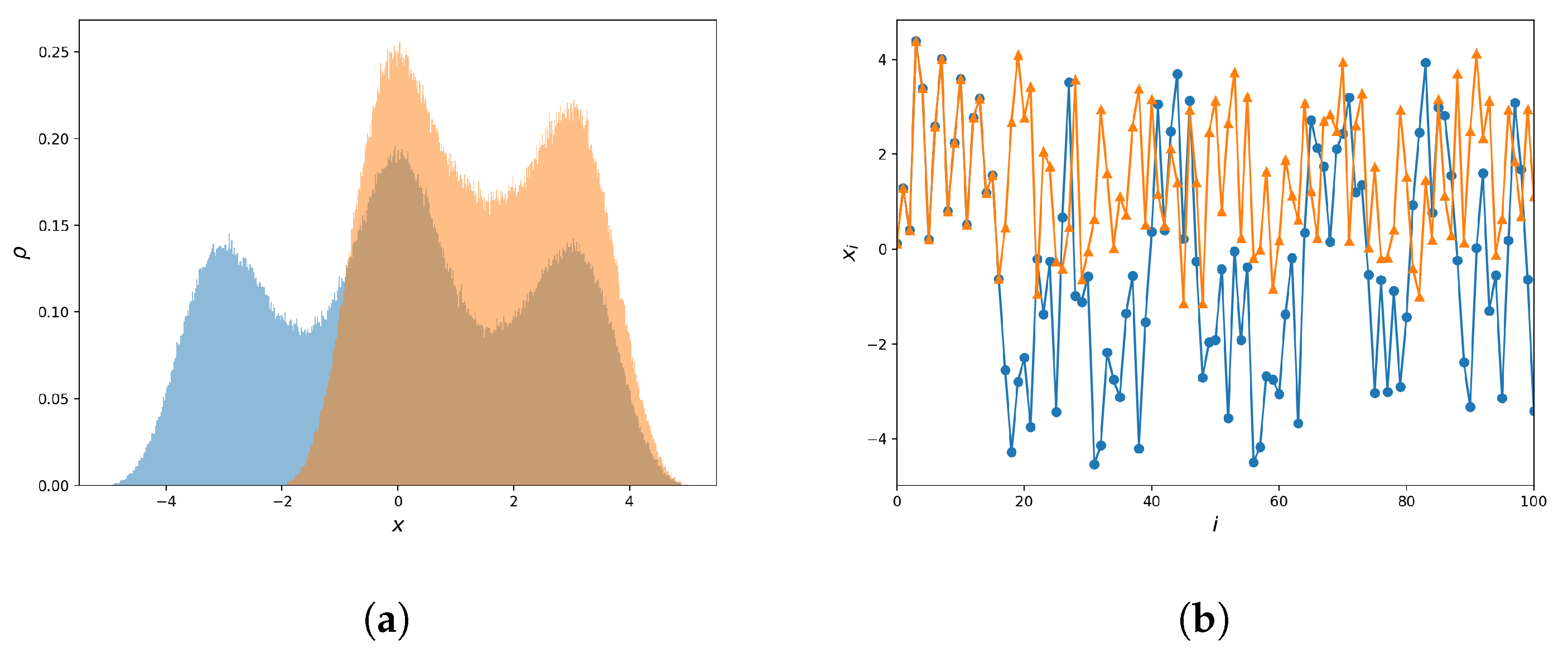
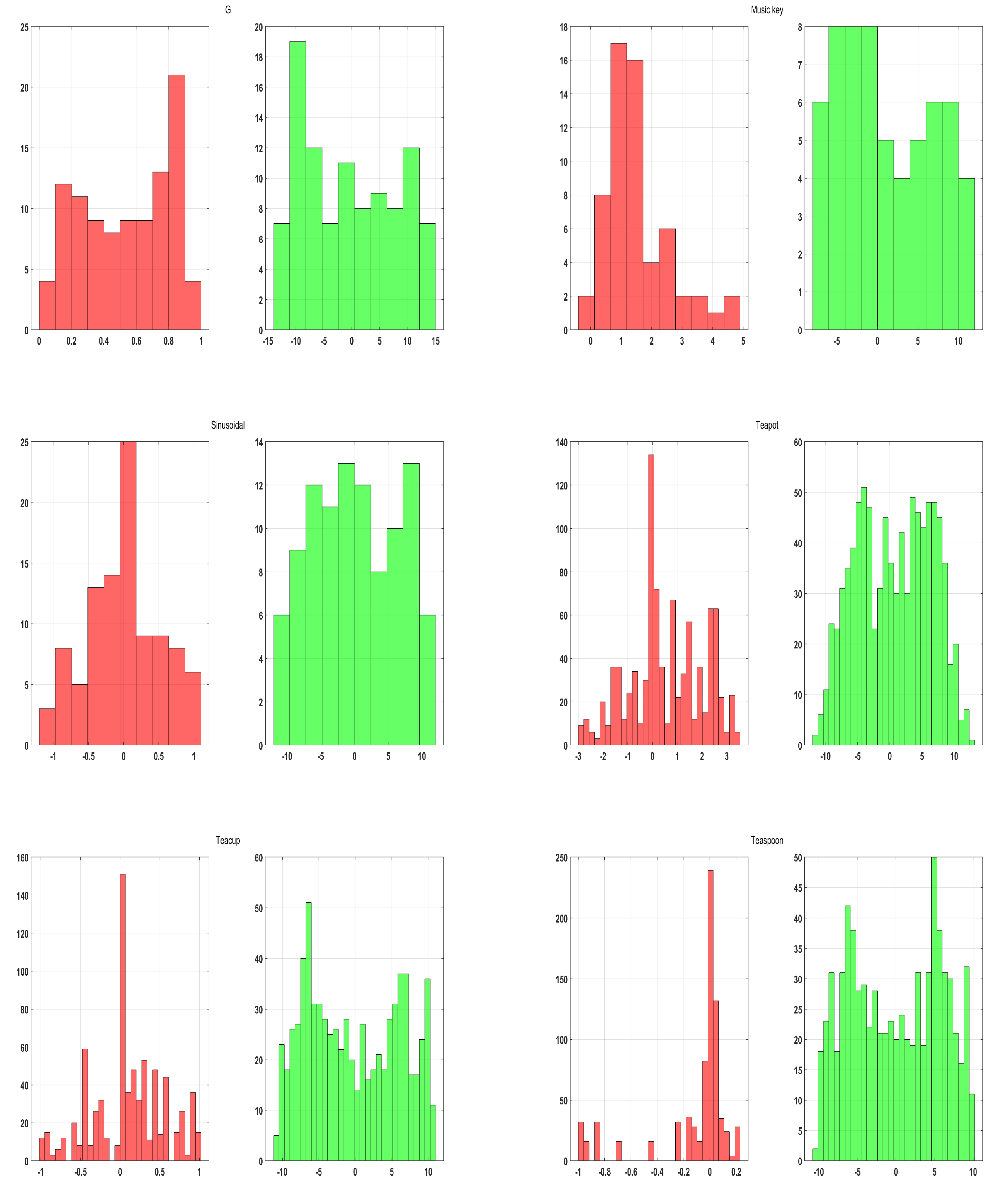
8.2. Histogram Analysis

Any statistically unbiased random time series should have a histogram that is uniform, indicating that there is no bias in the average values that occur over a specific subinterval of the state space. Here, the histograms were computed for the concatenated coordinate vectors ${\mathsf{\Pi }}_{row},{\mathsf{\Psi }}_{row}$. The row ${\mathsf{\Sigma }}_{row}$, being a shuffling of ${\mathsf{\Pi }}_{row}$, has the exact same histogram, so it is not shown here. The histograms are displayed in Figure 20. For the curves, the histogram consists of 10 groups, while for the surfaces, there are 30 groups. The ones corresponding to the ciphertext curves/patches are clearly more uniform compared to the plaintext ones.

Table 3. Histogram variance of the curves shown in Figure 16 and Figure 19.

	Original	Shuffled	Modulated
Curve 1 (G)	7.3333	7.3333	11.3333
Curve 2 (music key)	0.9290	0.9290	0.0572
Curve 3 (sinusoidal)	26.2222	26.2222	6.6667
Teapot	814.17	814.17	244.66
Teacup	646.78	646.78	88.6448
Teaspoon	2707.6	2707.6	70.593

also displays the histogram variance for three curves and shapes. The variance is much lower for the ciphertext points, indicating a more uniform histogram. Notice, however, that this analysis was performed in a very small ciphertext and, therefore, should only be interpreted as a measure of improved confusion in the ciphertext.

8.3. Correlation

Correlation indicates whether there is any linear relationship between two datasets. For two independent datasets, their correlation should be very close to zero, indicating that their values are linearly independent. Here, the correlation was measured between consecutive control points in the plaintext and ciphertext curves. Note here that, as a plaintext curve can have any form or shape, it is possible that the consecutive control points of the plaintext curve may also showcase low correlation. However, even in this case, it is expected that the correlation of the ciphertext control points will be even lower. The results are shown in

Table 4. Correlation of consecutive points for the curves shown in Figure 16 and Figure 19.

	Original	Shuffled	Modulated
Curve 1 (G)	0.9573	−0.1049	−0.0361
Curve 2 (music key)	0.9290	0.0812	0.0572
Curve 3 (sinusoidal)	0.8523	−0.0142	−0.1371
Teapot	0.9144	−0.0420	0.2114
Teacup	0.8356	0.0049	0.1822
Teaspoon	0.9788	0.0330	0.2180

.

8.4. Noise

The process of decryption described in Section 6.3 can be performed even if the ciphertext $\widehat{\mathsf{\Psi }}=\mathsf{\Psi }+\mathcal{W}$ has been corrupted by noise $\mathcal{W}$ during transmission. The noise will still be present in the decrypted set of control points though. When the channel noise is too intense, the decryption process can be independently complemented by a suitable filtering process to reduce the noise.

Figure 21 shows the result of decryption from a ciphertext set $\widehat{\mathsf{\Psi }}$ of control points under different noise intensities. The noise was modelled as uniform random numbers in the interval $[-z,z]$, where $z=0.001,0.01,0.1$ for the “G” curve and $z=0.01,0.1,0.5$ for the teapot. The error norms between the plaintext and decrypted control points are 0.0041, 0.0380, and 0.4505, respectively, for the “G” curve and 0.1043, 1.0768, 5.1801 for the teapot.

8.5. Key Space

The key space of the encryption (Section 6.2) is the same as the key space of the source map. As shown in Table 1, all the maps have the required key space to resist brute force attacks.

8.6. Key Sensitivity

The encryption process inherits the avalanche property of the chaotic map it uses as its source of randomness. As any chaotic map showcases sensitivity to parameter changes, perturbing any key value in (33) in the decryption process will result in the failure of the decryption. Figure 22 shows two such examples, were it can be observed that, indeed, the decryption fails to recreate the original plaintext curve and patch.

9. Conclusions and Future Goals

This work studied a chaotification technique, which is an extension of [18] and consists of combining the remainder of multiple scalings of the map’s value for the next iteration. The resulting maps can achieve a high Lyapunov exponent value, which can be controlled by appropriate parameter tuning.

An application of the proposed maps to the encryption of B-spline curves and patches was considered. The encryption consists of two steps: the first is the shuffling of the control points, and the second is an addition modulation step.

Future studies will be directed towards two main research areas. The first is the problem of chaotification. The use of the remainder operator will be explored for the creation of chaotic maps with a controllable mapping domain and without any equilibria. The control of the mapping interval will be of use in developing maps with modifiable statistical characteristics, which is desirable in various applications. The absence of equilibria is also desirable for achieving robust chaotic behaviour, as the Period 1 behaviour completely vanishes. Moreover, maps and systems without equilibria are themselves a distinct topic of study in dynamical systems’ analysis.

A second extension of this work is to generalise the encryption for rational B-spline curves and patches [30]. Here, the process should include the encryption of the control points along with the corresponding weights. Moreover, other types of geometric data structures can be considered, for example 3D objects. Finally, apart from the additive modulation, which is a linear operator, other operations can be considered for increased complexity, such as multiplication or cosine transformation. It must be noted though that highly nonlinear operations may introduce numerical errors during the decryption, so their choice must be carefully made. Any additional encryption steps can be considered either directly on the floating point plaintext data or in their binary representation. It would also be interesting to study if chaotic maps can be used for watermarking B-spline curves.

References

- Grassi, G. Chaos in the Real World: Recent Applications to Communications, Computing, Distributed Sensing, Robotic Motion, Bio-Impedance Modelling and Encryption Systems. Symmetry 2021, 13, 2151. [Google Scholar] [CrossRef]
- Moysis, L.; Butusov, D.N.; Tutueva, A.; Ostrovskii, V.; Kafetzis, I.; Volos, C. Introducing Chaos and Chaos Based Encryption Applications to University Students-Case Report of a Seminar. In Proceedings of the 2022 11th International Conference on Modern Circuits and Systems Technologies (MOCAST), Bremen, Germany, 8–10 June 2022; pp. 1–6. [Google Scholar]
- Özkaynak, F. Brief review on application of nonlinear dynamics in image encryption. Nonlinear Dyn. 2018, 92, 305–313. [Google Scholar] [CrossRef]
- Akmeşe, Ö.F. Bibliometric Analysis of Publications on Chaos Theory and Applications during 1987–2021. Chaos Theory Appl. 2022, 4, 169–178. [Google Scholar] [CrossRef]
- Natiq, H.; Banerjee, S.; Said, M. Cosine chaotification technique to enhance chaos and complexity of discrete systems. Eur. Phys. J. Spec. Top. 2019, 228, 185–194. [Google Scholar] [CrossRef]
- Hua, Z.; Zhou, B.; Zhou, Y. Sine chaotification model for enhancing chaos and its hardware implementation. IEEE Trans. Ind. Electron. 2018, 66, 1273–1284. [Google Scholar] [CrossRef]
- Hua, Z.; Zhang, Y.; Zhou, Y. Two-dimensional modular chaotification system for improving chaos complexity. IEEE Trans. Signal Process. 2020, 68, 1937–1949. [Google Scholar] [CrossRef]
- Mansouri, A.; Wang, X. A novel one-dimensional chaotic map generator and its application in a new index representation-based image encryption scheme. Inf. Sci. 2021, 563, 91–110. [Google Scholar] [CrossRef]
- Wu, Q. Cascade-sine chaotification model for producing chaos. Nonlinear Dyn. 2021, 106, 2607–2620. [Google Scholar] [CrossRef]
- Belazi, A.; Kharbech, S.; Aslam, M.N.; Talha, M.; Xiang, W.; Iliyasu, A.M.; Abd El-Latif, A.A. Improved Sine-Tangent chaotic map with application in medical images encryption. J. Inf. Secur. Appl. 2022, 66, 103131. [Google Scholar] [CrossRef]
- Lu, Q.; Yu, L.; Zhu, C. Symmetric Image Encryption Algorithm Based on a New Product Trigonometric Chaotic Map. Symmetry 2022, 14, 373. [Google Scholar] [CrossRef]
- Zhu, H.; Ge, J.; Qi, W.; Zhang, X.; Lu, X. Dynamic analysis and image encryption application of a sinusoidal-polynomial composite chaotic system. Math. Comput. Simul. 2022, 198, 188–210. [Google Scholar] [CrossRef]
- Hua, Z.; Zhou, Y. Exponential chaotic model for generating robust chaos. IEEE Trans. Syst. Man Cybern. Syst. 2019, 51, 3713–3724. [Google Scholar] [CrossRef]
- Zang, H.; Yuan, Y.; Wei, X. Research on Pseudorandom Number Generator Based on Several New Types of Piecewise Chaotic Maps. Math. Probl. Eng. 2021, 2021, 1375346. [Google Scholar] [CrossRef]
- Zhang, S.; Liu, L. A novel image encryption algorithm based on SPWLCM and DNA coding. Math. Comput. Simul. 2021, 190, 723–744. [Google Scholar] [CrossRef]
- Ablay, G. Lyapunov Exponent Enhancement in Chaotic Maps with Uniform Distribution Modulo One Transformation. Chaos Theory Appl. 2022, 4, 45–58. [Google Scholar] [CrossRef]
- Khairullah, M.K.; Alkahtani, A.A.; Bin Baharuddin, M.Z.; Al-Jubari, A.M. Designing 1D Chaotic Maps for Fast Chaotic Image Encryption. Electronics 2021, 10, 2116. [Google Scholar] [CrossRef]
- Moysis, L.; Kafetzis, I.; Baptista, M.S.; Volos, C. Chaotification of One-Dimensional Maps Based on Remainder Operator Addition. Mathematics 2022, 10, 2801. [Google Scholar] [CrossRef]
- Zhang, Z.; Zhu, H.; Ban, P.; Wang, Y.; Zhang, L.Y. Buffeting Chaotification Model for Enhancing Chaos and Its Hardware Implementation. IEEE Trans. Ind. Electron. 2022, 70, 2916–2926. [Google Scholar] [CrossRef]
- Zhu, M.; Wang, C. A novel parallel chaotic system with greatly improved Lyapunov exponent and chaotic range. Int. J. Mod. Phys. B 2020, 34, 2050048. [Google Scholar] [CrossRef]
- Dong, C.; Rajagopal, K.; He, S.; Jafari, S.; Sun, K. Chaotification of Sine-series maps based on the internal perturbation model. Results Phys. 2021, 31, 105010. [Google Scholar] [CrossRef]
- Lawnik, M.; Berezowski, M. New Chaotic System: M-Map and Its Application in Chaos-Based Cryptography. Symmetry 2022, 14, 895. [Google Scholar] [CrossRef]
- Ablay, G. Chaotic map construction from common nonlinearities and microcontroller implementations. Int. J. Bifurc. Chaos 2016, 26, 1650121. [Google Scholar] [CrossRef]
- Liu, L.; Wang, J. A cluster of 1D quadratic chaotic map and its applications in image encryption. Math. Comput. Simul. 2023, 204, 89–114. [Google Scholar] [CrossRef]
- Akgul, A.; Kacar, S.; Pehlivan, I.; Aricioglu, B. Chaos-based encryption of multimedia data and design of security analysis interface as an educational tool. Comput. Appl. Eng. Educ. 2018, 26, 1336–1349. [Google Scholar] [CrossRef]
- Abdallah, H.A.; Meshoul, S. A Multilayered Audio Signal Encryption Approach for Secure Voice Communication. Electronics 2023, 12, 2. [Google Scholar] [CrossRef]
- Wang, X.; Xu, M.; Li, Y. Fast encryption scheme for 3D models based on chaos system. Multimed. Tools Appl. 2019, 78, 33865–33884. [Google Scholar] [CrossRef]
- Gao, S.; Wu, R.; Wang, X.; Wang, J.; Li, Q.; Wang, C.; Tang, X. A 3D model encryption scheme based on a cascaded chaotic system. Signal Process. 2023, 202, 108745. [Google Scholar] [CrossRef]
- Gao, X.; Miao, M.; Chen, X. Multi-image encryption algorithm for 2D and 3D images based on chaotic system. Front. Phys. 2022, 10, 498. [Google Scholar] [CrossRef]
- Piegl, L.; Tiller, W. The NURBS Book; Springer Science & Business Media: Berlin/Heidelberg, Germany, 2012. [Google Scholar]
- Deng, C.; Lin, H. Progressive and iterative approximation for least squares B-spline curve and surface fitting. Comput.-Aided Des. 2014, 47, 32–44. [Google Scholar] [CrossRef]
- Hu, H.; Beck, J.; Lauer, M.; Stiller, C. Continuous Fusion of Motion Data Using an Axis-Angle Rotation Representation with Uniform B-spline. Sensors 2021, 21, 5004. [Google Scholar] [CrossRef]
- Majeed, A.; Abbas, M.; Qayyum, F.; Miura, K.T.; Misro, M.Y.; Nazir, T. Geometric modeling using new Cubic trigonometric B-spline functions with shape parameter. Mathematics 2020, 8, 2102. [Google Scholar] [CrossRef]
- Noreen, I. Collision free smooth path for mobile robots in cluttered environment using an economical clamped cubic B-spline. Symmetry 2020, 12, 1567. [Google Scholar] [CrossRef]
- Marinić-Kragić, I.; Perišić, S.; Vučina, D.; Ćurković, M. Superimposed RBF and B-spline parametric surface for reverse engineering applications. Integr.-Comput.-Aided Eng. 2020, 27, 17–35. [Google Scholar] [CrossRef]
- Zachariadis, O.; Teatini, A.; Satpute, N.; Gómez-Luna, J.; Mutlu, O.; Elle, O.J.; Olivares, J. Accelerating B-spline interpolation on GPUs: Application to medical image registration. Comput. Methods Programs Biomed. 2020, 193, 105431. [Google Scholar] [CrossRef]
- Hua, Z.; Zhou, Y. Image encryption using 2D Logistic-adjusted-Sine map. Inf. Sci. 2016, 339, 237–253. [Google Scholar] [CrossRef]
- Pareek, N.; Patidar, V.; Sud, K. Cryptography using multiple one-dimensional chaotic maps. Commun. Nonlinear Sci. Numer. Simul. 2005, 10, 715–723. [Google Scholar] [CrossRef]
- Alzaidi, A.A.; Ahmad, M.; Doja, M.N.; Al Solami, E.; Beg, M.S. A New 1D Chaotic Map and β-Hill Climbing for Generating Substitution-Boxes. IEEE Access 2018, 6, 55405–55418. [Google Scholar] [CrossRef]
- Moysis, L. Introduction to Computer Aided Geometric Design—A Student’s Companion with Matlab Examples. 2019. Available online: https://www.researchgate.net/profile/Lazaros-Moysis/publication/329337381_Introduction_to_Computer_Aided_Geometric_Design_-_A_student’s_companion_with_Matlab_examples_2nd_Edition/links/5c66dcfb4585156b57ffdffb/Introduction-to-Computer-Aided-Geometric-Design-A-students-companion-with-Matlab-examples-2nd-Edition.pdf (accessed on 30 January 2023).
- Burkardt, J. Teapot, Teacup, Teaspoon Data Files. 2006. Available online: https://people.sc.fsu.edu/~jburkardt/data/bezier_surface/bezier_surface.html (accessed on 30 January 2023).