Solving a System of Caputo Fractional-Order Volterra Integro-Differential Equations with Variable Coefficients Based on the Finite Difference Approximation via the Block-by-Block Method

Abstract

This paper focuses on computational technique to solve linear systems of Volterra integro-fractional differential equations (LSVIFDEs) in the Caputo sense for all fractional order $\mathrm{lins}\mathrm{in}\left(0,1\right]$ using two and three order block-by-block approach with explicit finite difference approximation. With this method, we aim to use an appropriate process to transform our problem into an analogous piecewise iterative linear algebraic system. Moreover, algorithms for treating LSVIFDEs using the above process have been developed, in order to express these solutions. In addition, numerical examples for our scheme are presented based on various kernels, including symmetry kernel and other sorts of separate kernels, are used to illustrate the validity, effectiveness and applicability of the suggested approach. Consequently, comparisons are performed with exact results using this technique, to communicate these approaches most general programs are written in Python V 3.8.8 software $\left(2021\right)$.

1. Introduction

A branch of mathematics known as Fractional Calculus (FC) may be thought of as the extension of integration and differentiation to arbitrary non-integer order. In the last few decades, there has been an increasing interest in the study of FC which is a valuable tool of applied mathematics for studying a variety of problems arising from the modeling of many phenomena in several branches of science and engineering, including mathematical physics, finance, hydrology, biophysics, thermodynamics, control theory, statistical mechanics, as well as astrophysics, cosmology and bioengineering, which are just a few of the real-world applications of fractional calculus (see, for instance, [1,2,3,4,5,6,7,8,9,10]). All modeling is based on the description of their properties in terms of fractional derivatives, naturally leading to the formation of fractional differential equations (FDEs) or fractional integro-differential equations (IFDEs). The fractional equations have attracted the interest of mathematicians and other scientists, leading to increased study of the FDE or IFDE solutions or a system of these in recent years [11,12,13,14]. Few of these equations can be solved explicitly, hence numerical approaches that are acceptable mixtures of numerical integrations and interpolation must often be used [15,16].

In addition, various research has been published for the creation of new techniques for finding numerical or approximate solutions, such as the Adomian decomposition method [17], homotopy perturbation method [18], collocation method [19] and Jacobi operational matrix method [20]. Muna, M. Mustafa and Thekra A. Latiff [21] used two and three points of the block-by-block method for solving the Volterra integral equations with delay. Katani and Shahmorad [22] used it to solve the systems of nonlinear Volterra integral equations. Miran and Shazad [23] applied the block-by-block method to solve linear Volterra integro fractional differential equations with a constant time-delay of retardation. Moreover, Atefa J. Salih [24] used second, third and fourth order block-by-block method for solving systems of nonlinear Volterra integro-differential equations.

In this work, the scheme was treated using a new procedure for finding the solutions of LSVI-FDEs based on explicit central finite difference approximation via the block-by-block method combined with adaptive Simpson’s method. The first step was described, summarized in a decent algorithm, and, ultimately, a computer program using Python-software was built.

The rest of this paper is structured as follows. After this introduction, definition of the work problem is presented in Section 2. Key properties with lemmas as well as some definitions and introductions to fractional calculus are offered in Section 3, and we outline the formulation of the essential quadrature formula principles that are applicable to our study. Section 4 derives the new scheme, which is based on the block-by-block method with explicit finite difference approximation. In Section 5, the performance of the suggested method is presented together with acceptable numerical results. The article concludes in Section 6 with conclusions.

2. Definition of the Problem

The goal of this paper is to provide a numerical scheme for solving a fractional order linear system Volterra integro-fractional differential equations (LSVIFDEs) of Caputo sense with variable coefficients in the following general form, for each $i=0,1,2,\dots ,m:$

$${{}_a{}^{c}D}_x^{{\alpha }_{in}}{y}_i\left(x\right)+{\displaystyle \sum _{k=1}^{n-1}}{\mathcal{P}}_{ik}\left(x\right){{}_a{}^{c}D}_x^{{\alpha }_{i(n-k)}}{y}_i\left(x\right)+{\mathcal{P}}_{in}\left(x\right)y_i\left(x\right)=f_i\left(x\right)+{\displaystyle \sum _{j=0}^m}{\lambda }_{ij}{\int }_a^x{\mathcal{K}}_{ij}\left(x,t\right){{}_a{}^{c}D}_t^{{\beta }_{i(m-j)}}{y}_j\left(t\right)dt.$$

(1)

Together, with the initial conditions:

$${\left[D_x^{{𝓋}_i}{y}_i\left(𝓍\right)\right]}_{x=a}=y_{i{𝓋}_i},{𝓋}_i=0,1,\dots ,{\mu }_i-1.$$

(2)

The variable coefficients ${\mathcal{P}}_{ik}\left(x\right)\in C\left(\mathbb{R}\right)$, which are real continuous functions, with ${\mathcal{P}}_{i0}\left(x\right)=1$ for all $i=0,1,2,\dots ,m$ and $k=0,1,\dots ,n.$ The fractional order $\left\{\left.{\alpha }_{ik},{\beta }_{ij}\right\}\in \left(0,1\right]\right.$ have the property that: ${\alpha }_{in}>{\alpha }_{i(n-1)}>\cdots >{\alpha }_{i1}>{\alpha }_{i0}=0$ and ${\beta }_{im}>{\beta }_{i(m-1)}>\cdots >{\beta }_{i1}>{\beta }_{i0}=0$. For all $i=0,1,2,\dots ,m,$ the ${\mu }_i=\max \left\{m_{ik}^{\alpha },m_{ij}^{\beta }\right\}$ for all $j=0,1,2,\dots ,m$ and $k=0,1,2,\dots ,n$ where $m_{ik}^{\alpha }-1<{\alpha }_{ik}\le m_{ik}^{\alpha }$ and $m_{ij}^{\beta }-1<{\beta }_{ij}\le m_{ij}^{\beta }.$ Furthermore, $y_i\left(𝓍\right)$ are the $\left(m+1\right)$-unknown real continuous functions which are the solution of LSVIFDEs (1), as well as, the functions $f_i\in C\left(\left[a,b\right],\mathbb{R}\right)$ and ${\mathcal{K}}_{ij}\in C(S,\mathbb{R})$ with $S=\left\{\left(𝓍,t\right):a\le t,𝓍\le b\right\}$ given functions. ${\lambda }_{ij}$ are the scalar parameter for all $i=0,1,2,\dots ,m$ and $j=0,1,2,\dots ,m$.

3. Preliminaries

3.1. Fractional Operators

In this segment, we first review the most common definitions and properties of fractional integration and derivatives with recall certain lemmas which will be used throughout this article. There are various definitions of fractional integration of real arbitrary order in the literature; however, they may not all be equivalent. The most popular definition is that of Riemann–Liouville, and it is as follows, while we begin by defining function space $C_{\gamma },\gamma \in \mathbb{R}$.

Definition 1 

([25]). A real valued function $y\left(x\right)$ defined on $[a,b]$, be in the space $C_{\gamma }\left[a,b\right],\gamma \in \mathbb{R}$ if there exists a real number $p>\gamma$, such that $y\left(x\right)={\left(x-a\right)}^p{y}_{*}\left(x\right),$ where $y_{*}\in C\left[a,b\right],$ and it is said to be in the space $C_{\gamma }^n\left[a,b\right]$, if $y^{\left(n\right)}\in C_{\gamma }\left[a,b\right],n\in {\mathbb{N}}_0$.

Definition 2 

([26]). The operator ${{}_{a}J}_x^{\alpha }y$ is the Riemann–Liouville fractional integral (R-L) of order $\alpha \in {\mathbb{R}}^{+}$ of a function $y\in C_{\mu },\mu \ge -1$ on a closed bounded interval $[a,b]$ is defined as:

$${{}_{a}J}_x^{\alpha }y\left(x\right)=\left\{\begin{array}{c}\frac{1}{\mathsf{\Gamma }\left(\alpha \right)}{\int }_a^x{\left(x-\vartheta \right)}^{\alpha -1}y\left(\vartheta \right)d\vartheta ,\alpha >0\\ y\left(x\right),\mathrm{whenver}\alpha =0\end{array}\right.$$

for all $\alpha ,\beta \ge 0$ have a semi-group property, that is: ${{}_{a}J}_x^{\alpha }{{}_{a}J}_x^{\beta }y\left(x\right){={}_{a}J}_x^{\alpha +\beta }y\left(x\right)={{}_{a}J}_x^{\beta }{{}_{a}J}_x^{\alpha }y\left(x\right)$. Respectively, here $\mathsf{\Gamma }$ represents the Euler’s Gamma function.

Definition 3 

([4,26]). The Caputo fractional derivative operator ${{}_a{}^{C}D}_x^{\alpha }$ of order $\alpha \in {\mathbb{R}}^{+}$ of a function $y\in C_{-1}^m$ on the closed bounded interval $[a,b]$ and $m-1<\alpha \le m,m\in {\mathbb{Z}}^{+}$ is defined as:

$${{}_a{}^{C}D}_x^{\alpha }y\left(x\right)=\left\{\begin{array}{c}{{}_{a}J}_x^{m-\alpha }\left[D_x^{m}y\left(x\right)\right]\\ \hspace{1em}\hspace{1em}=\frac{1}{\mathsf{\Gamma }\left(m-\alpha \right)}{\int }_a^x{\left(x-\vartheta \right)}^{m-\alpha -1}{y}^{\left(m\right)}\left(\vartheta \right)d\vartheta ,\alpha >0,x>a\\ y\left(x\right),\mathrm{whenever}\alpha =0\\ y^{\left(m\right)}\left(x\right),\mathrm{If}\alpha =m\left(\in {\mathbb{Z}}^{+}\right)\mathrm{and}y\in C^m\left[a,b\right]\end{array}\right.$$

Additionally, for $\alpha >0$, the Caputo fractional derivative of a constant function is equal to zero, it means ${}_a{}^c{D}_{𝓍}^{\alpha }\mathcal{A}=0,$ for any constant $\mathcal{A}.$ If $y\left(x\right)$ is continuous $\alpha \ge 0$ with $n-1<\alpha \le n,n\in \mathbb{N},$ then ${{}_a{}^{C}D}_x^{\alpha }{{}_{a}J}_x^{\alpha }y\left(x\right)=y\left(x\right),x\in \left[a,b\right]$. Additionally, assume that $\alpha \ge 0,y\left(x\right)\in C^{⌈\alpha ⌉}\left[a,b\right],$ then

$${{}_{a}J}_x^{\alpha }{{}_a{}^{C}D}_x^{\alpha }y\left(x\right)=y\left(x\right)-{\sum }_{k=0}^{⌈\alpha ⌉-1}\frac{y^{\left(k\right)}\left(a\right)}{k!}{\left(x-a\right)}^k$$

Lemma 1 

([26]). Let $y\left(𝓍\right)={(𝓍-a)}^v,v\ge 0$ and The Caputo derivative of order $\alpha \ge 0$ is given by:

$${{}_a{}^{C}D}_{𝓍}^{\alpha }y\left(𝓍\right)=\left\{\begin{array}{c}0\hspace{1em}\hspace{1em}\hspace{1em}\hspace{1em}\hspace{1em}\hspace{1em}\hspace{1em}\mathrm{if}v\in \{0,1,2,\dots ,⌈\alpha ⌉-1\}\\ \frac{Г\left(v+1\right)}{Г\left(v+1-\alpha \right)}{\left(𝓍-a\right)}^{v-\alpha } \mathrm{if}v\in \mathbb{N}\mathrm{and}v\ge ⌈\alpha ⌉\\ \hspace{1em}\hspace{1em}\hspace{1em}\hspace{1em}\hspace{1em}\hspace{1em}\hspace{1em}\mathrm{or} v\notin \mathbb{N} \mathrm{and} v>⌈\alpha ⌉-1\\ \end{array}\right.$$

Lemma 2 

([14]). Let $\alpha \ge 0,\alpha \notin \mathbb{N}$ and $m=⌈\alpha ⌉.$ Moreover, assume that $y\in C_{-1}^m\left[a,b\right].$ Then the Caputo fractional derivative ${{}_a{}^{C}D}_x^{\alpha }y\left(x\right)$ is continuous on $\left[a,b\right]$ and ${\left[{{}_a{}^{C}D}_x^{\alpha }y\left(x\right)\right]}_{x=a}=0.$

Lemma 3 

([26,27]). The finite difference approximation of Caputo derivative for $0<\alpha \le 1$ at given points $x=x;r=0,1,\dots ,N-1$ and $h=(b-a)/N,(N\in {\mathbb{Z}}^{+})$ is of the form

$${{}_a{}^{C}D}_x^{\alpha }y\left(x_{r+1}\right)=\frac{h^{-\alpha }}{\mathsf{\Gamma }(2-\mathsf{\alpha })}{\displaystyle \sum _{s=0}^r}\left[y\left(x_{r-s+1}\right)-y\left(x_{r-s}\right)\right]b_s^{\alpha }$$

where $b_s^{\alpha }={(s+1)}^{1-\alpha }-s^{1-\alpha }$.

Lemma 4 

([23]). For any $p$-orders of block-by-block methods the Caputo fractional derivative of order $0<\alpha \le 1$ for any smooth function $y\left(x\right)$ on $\left[a,b\right]$, can evaluate it at any points $x=x_{rp+\vartheta }$ for each $r=0,1,\dots ,N-1(N\in {\mathbb{Z}}^{+})$ with $\vartheta =1,2,\dots ,p$ by the following formula:

$$\begin{array}{c}{\left.{{}_a{}^{C}D}_x^{\alpha }y\left(x\right)\right|}_{x=x_{rp+\vartheta }}\\ \hspace{1em}\hspace{1em}\hspace{1em}\hspace{1em}=\frac{{\left[\stackrel{-}{h}\right]}^{-\alpha }}{\mathsf{\Gamma }\left(2-\mathsf{\alpha }\right)}\left\{\left[y\left(x_{rp+\vartheta }\right)\right.-y\left(x_{rp+\vartheta -1}\right)]+{\displaystyle \sum _{s=1}^{pr+\vartheta -1}}\left[{y(x}_{rp+\vartheta -s})-{y(x}_{rp+\vartheta -(s+1)})\right]b_s^{\alpha }\right\}\end{array}$$

where $b_s^{\alpha }={(s+1)}^{1-\alpha }-s^{1-\alpha },\stackrel{-}{h}=\frac{b-a}{pN},p\in {\mathbb{Z}}^{+}$.

3.2. Review Some of Integrated Formulas: [23,24,25,28]

In this section we explain the most important rules in quadrature formulas which are Simpson’s $\frac{1}{3}h$ and Adaptive Simpson’s rules. The following formula is derived by using adaptive Simpson’s rule:

$${\int }_{x_r}^{x_{r+1}}f\left(x\right)dx\cong \frac{h}{6}\left[f\left(x_r\right)+4f\left(x_{r+1/2}\right)+f\left(x_{r+1}\right)\right]$$

(3)

where $f\left(x_{r+1/2}\right)$ can be found from the Newton-Gregory Forward-Difference formula:

$$P_n\left(x\right)=f_r+\left(\genfrac{}{}{0pt}{}{s}{1}\right)∆f_r+\left(\genfrac{}{}{0pt}{}{s}{2}\right){∆}^2{f}_r+\left(\genfrac{}{}{0pt}{}{s}{3}\right){∆}^3{f}_r+\cdots +\left(\genfrac{}{}{0pt}{}{s}{n}\right){∆}^n{f}_r$$

where

$$f_r=f\left(x_r\right),x_s=x_r+sh,s=\frac{x-x_r}{h};{∆}^n{f}_r={∆}^{n-1}{f}_{r+1}-{∆}^{n-1}{f}_r;n\ge 1$$

Hence putting $s=\frac{1}{2}$ and $n=2$ so to interpolate $f\left(x_{r+1/2}\right)$ by $P_2\left(x=x_s\right)$, thus:

$$f\left(x_{r+1/2}\right)\cong P_2\left(x+\frac{1}{2}h\right)=\frac{3}{8}{f}_r+\frac{3}{4}{f}_{r+1}-\frac{1}{8}{f}_{r+2}$$

(4)

If we take $n=3$ and also interpolate $f\left(x_{r+1/2}\right)$ by $P_3\left(x=x_s\right)$ we obtain:

$$f\left(x_{r+1/2}\right)\cong P_3\left(x_r+\frac{1}{2}h\right)=\frac{1}{16}\left[5f_r+15f_{r+1}-5f_{r+2}+f_{r+3}\right]$$

(5)

4. Proposed Method

The main objective of this section is to create a new strategy for treating the equation LSVIFDE which build by combining block-by-block techniques of difference block orders (two and three) with aid of forward finite difference approximation. The general form:

$${{}_a{}^{c}D}_x^{{\alpha }_{in}}{y}_i\left(x\right)+{\displaystyle \sum _{k=1}^{n-1}}{\mathcal{P}}_{ik}\left(x\right){{}_a{}^{c}D}_x^{{\alpha }_{i(n-i)}}{y}_i\left(x\right)+{\mathcal{P}}_{in}\left(x\right)y_i\left(x\right)=f_i\left(x\right)+{\displaystyle \sum _{j=0}^m}{\lambda }_{ij}{\int }_a^x{\mathcal{K}}_{ij}\left(x,t\right){{}_a{}^{c}D}_t^{{\beta }_{i(m-j)}}{y}_j\left(t\right)dt$$

Now, for all fractional orders $\left\{{\alpha }_{in}\mathrm{a}\mathrm{n}\mathrm{d}{\beta }_{im}\right\}$ lies in $\left(0,1\right]$, thus ${\mu }_i=\max \left\{⌈{\alpha }_{in}⌉,⌈{\beta }_{im}⌉\right\}=1$ so the conditions (2) become: $y_i\left(a\right)=y_{i0}\left(\in \mathbb{R}\right),\mathrm{for} \mathrm{all} i=0,1,2,\dots ,m$ on the range $a\le x\le b$.

In our techniques, we begin by dividing the interval $\left[a,b\right]$ into $N$-equal sub-intervals, each of them is then divided into $p$-subinterval, $p$ is any positive integer number, on length $h$ such that: $h=\left(b-a\right)/Np$. Also, for $pr<s\le p\left(r+1\right);r=0,1,2,\dots ,N-1$ and set $x=x_s$ in system (1), so we can write:

$$\begin{array}{cc}\hfill {\left[{{}_a{}^{c}D}_x^{{\alpha }_{in}}{y}_i\left(x\right)\right]}_{x=x_s}& +{\displaystyle \sum _{k=1}^{n-1}}{\mathcal{P}}_{ik}\left(x_s\right){\left[{{}_a{}^{c}D}_x^{{\alpha }_{i\left(n-k\right)}}{y}_i\left(x\right)\right]}_{x=x_s}+{\mathcal{P}}_{in}\left(x_s\right)y_i\left(x_s\right)\hfill \\ & =f_i\left(x_s\right)+{\displaystyle \sum _{j=0}^m}{\lambda }_{ij}{\int }_a^{x_{pr}}{\mathcal{K}}_{ij}\left(x_s,t\right){{}_a{}^{c}D}_t^{{\beta }_{i\left(m-j\right)}}{y}_j\left(t\right)dt\hfill \\ & +{\displaystyle \sum _{j=0}^m}{\lambda }_{ij}{\int }_{x_{pr}}^{x_s}{\mathcal{K}}_{ij}\left(x_s,t\right){{}_a{}^{c}D}_t^{{\beta }_{i\left(m-j\right)}}{y}_j\left(t\right)dt\hfill \end{array}$$

(6)

where ${\mathcal{P}}_{i0}\left(x\right)=1$ for all $i=0,1,2,\dots ,m.$ Now, by applying the block-step idea [23,24], at each sub-interval in the points $x=x_{pr+1},x_{pr+2},x_{pr+3},\dots ,x_{pr+p}=x_{p(r+1)}$ for each $p$-blocks order at each subinterval $\left[x_{pr},x_{p\left(r+1\right)}\right]$ for each equations in the system (1). Apply the Lemma 4 for all fractional parts in the left-hand sides of our equation and we use the quadrature rules to approximate the integral terms: Simpson’s $\frac{1}{3}h$ and Adaptive Simpson’s rules, respectively. Noting that the first integral is vanishes at $r=0$.

4.1. Two-Block Method

Using the basic technique for the two-block method, where $p=2$ and for each equations, thus for each index $r=0,1,2,\dots ,N-1$, Simpson’s rule may be used to integrate over $\left[a,x_{2r}\right]$; at points $x_{2r},x_{2r+1}\mathrm{a}\mathrm{n}\mathrm{d}{x}_{2r+2}$, a quadratic interpolation polynomial is used to approximate the integrand over the interval $\left[x_{2r},x_{2r+1}\right]$; and Simpson’s rule can also be used to integrate over $\left[x_{2r},x_{2r+2}\right]$. Furthermore, we approximate the fractional differential by using forward difference in Lemma 4 also using Equations (3) and (4). Thus, after some manipulations on system (6) we obtain the following two basic blocks. For each $i=\overline{0:m}$ and for each $r=\overline{0,N-1}$: The First block at point $(2r+1)$ became:

$$\begin{array}{c}\left\{{{}_{\mathcal{C}}{}^{0}G}_{n,1}^{i,\alpha }\left(r\right)-\frac{{\lambda }_{ii}h}{6}\left(4{{\mathcal{H}}_{m,i}^{i,\beta }\mathcal{K}}_i^i\left(x_{2r+1},t_{2r+1/2}\right)\left[\frac{3}{4}-\frac{1}{8}{\mathcal{C}}_{m,i}^{i,\beta }\left(1\right)\right]+{{\mathcal{H}}_{m,i}^{i,\beta }\mathcal{K}}_i^i\left(x_{2r+1},t_{2r+1}\right)\right)\right\}{y}_{i,2r+1}\hfill \\ \hspace{1em}\hspace{1em}\hspace{1em}+\frac{{\lambda }_{ii}h}{12}\left\{{\mathcal{H}}_{m,i}^{i,\beta }{\mathcal{K}}_i^i\left(x_{2r+1},t_{2r+1/2}\right)\right\}{y}_{i,2r+2}\hfill \\ \hspace{1em}\hspace{1em}\hspace{1em}-\frac{h}{6}{\displaystyle \sum _{j=0,j\ne i}^m}\left\{{\lambda }_{ij}\left(4{{\mathcal{H}}_{m,j}^{i,\beta }\mathcal{K}}_j^i\left(x_{2r+1},t_{2r+1/2}\right)\left[\frac{3}{4}-\frac{1}{8}{\mathcal{C}}_{m,j}^{i,\beta }\left(1\right)\right]+{{\mathcal{H}}_{m,j}^{i,\beta }\mathcal{K}}_j^i\left(x_{2r+1},t_{2r+1}\right)\right)\right\}{y}_{j,2r+1}\hfill \\ \hspace{1em}\hspace{1em}\hspace{1em}+\frac{h}{12}{\displaystyle \sum _{j=0,j\ne i}^m}\left\{{\lambda }_{ij}{\mathcal{H}}_{m,j}^{i,\beta }{\mathcal{K}}_j^i\left(x_{2r+1},t_{2r+1/2}\right)\right\}{y}_{j,2r+2}\hfill \\ ={\mathcal{F}}_{r,1}^i+\left\{{{}_{\mathcal{C}}{}^{0}G}_{n,1}^{i,\alpha }\left(r\right)-{}^1{\mathcal{P}}_n^i\left(r\right)\right\}{y}_{i,2r}-\frac{h}{6}{\displaystyle \sum _{j=0}^m}{\lambda }_{ij}\left\{4{\mathcal{H}}_{m,j}^{i,\beta }{\mathcal{K}}_j^i\left(x_{2r+1},t_{2r+1/2}\right)\left[\frac{3}{4}-\frac{1}{8}{\mathcal{B}}_{m,j}^{i,\beta }\left(1\right)\right]+{{\mathcal{H}}_{m,j}^{i,\beta }\mathcal{K}}_j^i\left(x_{2r+1},t_{2r+1}\right)\right\}{y}_{j,2r}\hfill \\ \hspace{1em}\hspace{1em}\hspace{1em}-{\displaystyle \sum _{\ell =1}^{2r}}\left[y_{i,2r-\ell +1}-y_{i,2r-\ell }\right]\left({{}_{\mathcal{B}}{}^{\ell }G}_{n,1}^{i,\alpha }\left(r\right)-{}^1{\mathcal{P}}_n^i\left(r\right)\right)\hfill \\ +{\displaystyle \sum _{j=0}^m}{\lambda }_{ij}\{\frac{h}{3}{\displaystyle \sum _{d=1}^{2r}}{w}_d{{\mathcal{H}}_{m,j}^{i,\beta }\mathcal{K}}_j^i\left(x_{2r+1},t_d\right)\left({\displaystyle \sum _{\ell =0}^{d-1}}\left[y_{j,d-\ell }-y_{j,d-\ell -1}\right]{\mathcal{B}}_{m,j}^{i,\beta }\left(\ell \right)\right)\hfill \\ \hspace{1em}\hspace{1em}\hspace{1em}+\frac{h}{6}({\mathcal{H}}_{m,j}^{i,\beta }{\mathcal{K}}_j^i\left(x_{2r+1},t_{2r}\right)\left[{\displaystyle \sum _{\ell =0}^{2r-1}}\left[y_{j,2r-\ell }-y_{j,2r-\ell -1}\right]{\mathcal{B}}_{m,j}^{i,\beta }\left(\ell \right)\right]\hfill \\ \hspace{1em}\hspace{1em}\hspace{1em}+4{\mathcal{H}}_{m,j}^{i,\beta }{\mathcal{K}}_j^i(x_{2r+1},t_{2r+1/2})[\frac{3}{8}{\displaystyle \sum _{\ell =0}^{2r-1}}\left[y_{j,2r-\ell }-y_{j,2r-\ell -1}\right]{\mathcal{B}}_{m,j}^{i,\beta }\left(\ell \right)+\frac{3}{4}{\displaystyle \sum _{\ell =1}^{2r}}\left[y_{j,2r-\ell +1}-y_{j,2r-\ell }\right]{\mathcal{B}}_{m,j}^{i,\beta }\left(\ell \right)\hfill \\ \hspace{1em}\hspace{1em}\hspace{1em}-\frac{1}{8}{\displaystyle \sum _{\ell =2}^{2r+1}}\left[y_{j,2r-\ell +2}-y_{j,2r-\ell +1}\right]{\mathcal{B}}_{m,j}^{i,\beta }\left(\ell \right)]+{\mathcal{H}}_{m,j}^{i,\beta }{\mathcal{K}}_j^i\left(x_{2r+1},t_{2r+1}\right)\left[{\displaystyle \sum _{\ell =1}^{2r}}\left[y_{j,2r-\ell +1}-y_{j,2r-\ell }\right]{\mathcal{B}}_{m,j}^{i,\beta }\left(\ell \right)\right])\}\hfill \end{array}$$

(7)

The Second block at point $(2r+2)$ became:

$$\begin{array}{c}\left\{\left({{}_{\mathcal{C}}{}^{1}G}_{n,2}^{i,\alpha }\left(r\right)-{}^2{\mathcal{P}}_n^i\left(r\right)\right)-\frac{{\lambda }_{ii}h}{3}\left({\stackrel{-}{w}}_{2r+1}{{\mathcal{H}}_{m,i}^{i,\beta }\mathcal{K}}_i^i\left(x_{2r+2},t_{2r+1}\right){+\stackrel{-}{w}}_{2r+2}{{\mathcal{H}}_{m,i}^{i,\beta }\mathcal{K}}_i^i\left(x_{2r+2},t_{2r+2}\right){\mathcal{C}}_{m,i}^{i,\beta }\left(1\right)\right)\right\}{y}_{i,2r+1}\\ +\left\{{{}_{\mathcal{C}}{}^{0}G}_{n,2}^{i,\alpha }\left(r\right)-\frac{{\lambda }_{ii}h}{3}{\stackrel{-}{w}}_{2r+2}{\mathcal{H}}_{m,i}^{i,\beta }{\mathcal{K}}_i^i\left(x_{2r+2},t_{2r+2}\right)\right\}{y}_{i,2r+2}\\ -\frac{h}{3}{\displaystyle \sum _{j=0,j\ne i}^m}\left\{{\lambda }_{ij}\left({\stackrel{-}{w}}_{2r+1}{{\mathcal{H}}_{m,j}^{i,\beta }\mathcal{K}}_j^i\left(x_{2r+2},t_{2r+1}\right){+\stackrel{-}{w}}_{2r+2}{{\mathcal{H}}_{m,j}^{i,\beta }\mathcal{K}}_j^i\left(x_{2r+2},t_{2r+2}\right){\mathcal{C}}_{m,j}^{i,\beta }\left(1\right)\right)\right\}{y}_{j,2r+1}\\ -\frac{h}{3}{\displaystyle \sum _{j=0,j\ne i}^m}\left\{{\lambda }_{ij}{\stackrel{-}{w}}_{2r+2}{{\mathcal{H}}_{m,j}^{i,\beta }\mathcal{K}}_j^i\left(x_{2r+2},t_{2r+2}\right)\right\}{y}_{j,2r+2}\\ ={\mathcal{F}}_{r,2}^i+\left\{{{}_{\mathcal{B}}{}^{1}G}_{n,2}^{i,\alpha }\left(r\right)-{}^2{\mathcal{P}}_n^i\left(r\right)\right\}{y}_{i,2r}\\ -\frac{h}{3}{\displaystyle \sum _{j=0}^m}\left\{{\lambda }_{ij}\left({\stackrel{-}{w}}_{2r+1}{{\mathcal{H}}_{m,j}^{i,\beta }\mathcal{K}}_j^i\left(x_{2r+2},t_{2r+1}\right)+{\stackrel{-}{w}}_{2r+2}{{\mathcal{H}}_{m,j}^{i,\beta }\mathcal{K}}_j^i\left(x_{2r+2},t_{2r+2}\right){\mathcal{B}}_{m,j}^{i,\beta }\left(1\right)\right)\right\}{y}_{j,2r}\\ -{\displaystyle \sum _{\ell =2}^{2r+1}}\left[y_{i,2r-\ell +2}-y_{i,2r-\ell +1}\right]\left({{}_{\mathcal{B}}{}^{\ell }G}_{n,2}^{i,\alpha }\left(r\right)-{}^2{\mathcal{P}}_n^i\left(r\right)\right)\\ +\frac{h}{3}{\displaystyle \sum _{j=0}^m}{\lambda }_{ij}\{{\stackrel{-}{w}}_{2r+1}{\mathcal{H}}_{m,j}^{i,\beta }{\mathcal{K}}_j^i\left(x_{2r+2},t_{2r+1}\right)\left({\displaystyle \sum _{\ell =1}^{2r}}\left[y_{j,2r-\ell +1}-y_{j,2r-\ell }\right]{\mathcal{B}}_{m,j}^{i,\beta }\left(\ell \right)\right)\\ +{\stackrel{-}{w}}_{2r+2}{\mathcal{H}}_{m,j}^{i,\beta }{\mathcal{K}}_j^i\left(x_{2r+2},t_{2r+2}\right)\left({\displaystyle \sum _{\ell =2}^{2r+1}}\left[y_{j,2r-\ell +2}-y_{j,2r-\ell +1}\right]{\mathcal{B}}_{m,j}^{i,\beta }\left(\ell \right)\right)\\ +{\displaystyle \sum _{d=1}^{2r}}{\stackrel{-}{w}}_d{{\mathcal{H}}_{m,j}^{i,\beta }\mathcal{K}}_j^i\left(x_{2r+2},t_d\right)\left({\displaystyle \sum _{\ell =0}^{d-1}}\left[y_{j,d-\ell }-y_{j,d-\ell -1}\right]{\mathcal{B}}_{m,j}^{i,\beta }\left(\ell \right)\right)\}c\end{array}$$

(8)

where for all $i=0,1,2,\dots ,m$ and $r=0,1,2,\dots ,N-1$:

$$\begin{array}{c}{\mathcal{F}}_{r,v}^i=f_i\left(t_0+\left(2r+\vartheta \right)h\right),\vartheta =1,2\\ \begin{array}{c}{\mathcal{H}}_{𝓀,\ell }^{i,\sigma }=\frac{h^{-{\sigma }_{i(𝓀-\ell )}}}{\mathsf{\Gamma }\left(2-{\sigma }_{i(𝓀-\ell )}\right)},\ell =0,1,\dots ,𝓀-1\\ \end{array}\end{array}$$

(9)

For all fractional orders $\sigma$ equal to $\left\{\alpha \mathrm{o}\mathrm{r}\beta \right\}$ and $𝓀$ equal to $\left\{n\mathrm{o}\mathrm{r}m\right\}$, respectively. Furthermore, $\mathcal{E}$ may be select $\left\{\mathcal{C}\mathrm{o}\mathrm{r}\mathcal{B}\right\}$, that

$${{}_{\mathcal{E}}{}^{𝓆}G}_{𝓀,v}^{i,\sigma }\left(r\right)={}^v{\mathcal{P}}_{𝓀}^i\left(r\right)+{\displaystyle \sum _{\ell =0}^{k-1}}{}^v{\mathcal{P}}_{\ell }^i\left(r\right){\mathcal{H}}_{𝓀,\ell }^{i,\sigma }{\mathcal{E}}_{𝓀,\ell }^{i,\sigma }\left(𝓆\right)$$

(10)

While, ${}^v{\mathcal{P}}_{\ell }^i\left(r\right)={\mathcal{P}}_{i\ell }\left(t_{pr+v}\right)={\mathcal{P}}_{i\ell }\left(t_0+\left(pr+v\right)h\right);h=\left(b-a\right)/2N$ and ${\mathcal{P}}_{i0}\equiv 1$. With,

$$\left.\begin{array}{c}\begin{array}{c}{\mathcal{C}}_{𝓀,\ell }^{i,\sigma }\left(𝓆\right)={\mathcal{B}}_{𝓀,\ell }^{i,\sigma }\left(𝓆\right)-{\mathcal{B}}_{𝓀,\ell }^{i,\sigma }\left(𝓆-1\right)\\ {\mathcal{B}}_{𝓀,\ell }^{i,\sigma }\left(𝓆\right)={\left(\gamma +1\right)}^{1-{\sigma }_{i(𝓀-\ell )}}-{\gamma }^{1-{\sigma }_{i(𝓀-\ell )}}\end{array}\\ \begin{array}{cc}{\mathcal{B}}_{n,k}^{i,\alpha }\left(-1\right)=0& \begin{array}{cc}\mathrm{a}\mathrm{n}\mathrm{d}& {\mathcal{B}}_{m,j}^{i,\beta }\left(-1\right)=0\end{array}\end{array}\end{array}\right\},\gamma ,𝓆=0,1,2,\dots$$

(11)

For all $i,j,\ell =0,1,\dots ,m$ and $𝓀=0,1,\dots ,\left\{norm\right\}$. Moreover,

$$\left.\begin{array}{c}{w}_0=w_{2r}=1,{\stackrel{-}{w}}_0={\stackrel{-}{w}}_{2r+2}=1\\ w_d=3-{\left(-1\right)}^d\mathrm{w}\mathrm{h}\mathrm{e}\mathrm{r}\mathrm{e}d=1,2,3,\dots ,2r-1\\ {\stackrel{-}{w}}_d=3-{\left(-1\right)}^d\mathrm{w}\mathrm{h}\mathrm{e}\mathrm{r}\mathrm{e}d=1,2,3,\dots ,2r+1\end{array}\right\}$$

(12)

As a result, at each step (at each $r$), we get $2(m+1)$ simultaneous equations with the same number of unknown functions, i.e., we will have two-block systems with $2(m+1)$ unknowns from Equations (7) and (8). As a consequence, we must establish the block of unknowns $\boxed{\begin{array}{c}{y}_{i,2r+1}\\ y_{i,2r+2}\end{array}}$ and $\boxed{\begin{array}{c}{y}_{j,2r+1}\\ y_{j,2r+2}\end{array}}$ with all $j=\overline{0:m}\mathrm{a}\mathrm{n}\mathrm{d}j\ne i$ for all $r=\overline{0:N-1}$ with each $i=\overline{0:m}$. So, in order to obtain the solution of the linear system of VIFDEs using the Python program (V 3.8.8), we wrote the following algorithm (BMP2).

Algorithm 1: Two-Block Method (BMP2)

Step 1: For each $i=0,1,\dots ,m:$ Set $T\left[i,0\right]=y_{i0}=y_i\left(t_0\right)$ [Are given from initial conditions]. Let $h=\left(b-a\right)/2N,N\in {\mathbb{Z}}^{+}.$ Step 2: for each $i=0,1,2,\dots ,m$: Calculate ${\mathcal{H}}_{n,k}^{i,\alpha }\mathrm{a}\mathrm{n}\mathrm{d}{\mathcal{H}}_{m,j}^{i,\beta }$ for $k=\overline{0:n}$ and $j=\overline{0:m}$ from the Equation (9). Determine ${}^v{\mathcal{P}}_k^i\left(r\right)$ for $=0,1,\dots ,n$; $r=0,1,\dots ,N-1$ and each $v=1,2$. Applying Equation (10) and step (2, i) to compute ${{}_{\mathcal{C}}{}^{𝓆}G}_{n,v}^{i,\alpha }\left(r\right),{{}_{\mathcal{B}}{}^{\ell }G}_{n,v}^{i,\alpha }\left(r\right)$ for all $=0,1,\dots ,N-1$; $𝓆=0,1$; $\ell \ge 1$ and for each $v=1,2$. Compute ${\mathcal{C}}_{m,i}^{i,\beta }\left(1\right)$ and ${\mathcal{B}}_{m,j}^{i,\beta }\left(\ell \right)$ for all $=0,1,2,\dots$; and $i,j=\overline{0:m}$ with all $\ell \ge 1$ from the Equation (11). Evaluate ${\mathcal{F}}_{r,v}^i$ for all $r=0,1,\dots ,N-1$ and each $v=1,2.$ For all $\mathit{r}=0,1,2,\dots ,\mathit{N}-1,$ doing steps 3–8: Step 3: For each $i=0,1,\dots ,m$: For each $j=\overline{0:m},$ compute $Q_i^1\left[j,r\right]=-\frac{{\lambda }_{ij}h}{6}\left\{4{\mathcal{H}}_{m,j}^{i,\beta }{\mathcal{K}}_j^i\left(x_{2r+1},t_{2r+1/2}\right)\left[\frac{3}{4}-\frac{1}{8}{\mathcal{C}}_{m,j}^{i,\beta }\left(1\right)\right]+{\mathcal{H}}_{m,j}^{i,\beta }{\mathcal{K}}_j^i\left(x_{2r+1},t_{2r+1}\right)\right\}$ and $R_i^1\left[j,r\right]=\frac{{\lambda }_{ij}h}{12}\left\{{\mathcal{H}}_{m,j}^{i,\beta }{\mathcal{K}}_j^i\left(x_{2r+1},t_{2r+1/2}\right)\right\}$. For each $j=\overline{0:m},$ evaluate $C_i^1\left[j,r\right]=\frac{{\lambda }_{ij}h}{6}\left\{4{\mathcal{H}}_{m,j}^{i,\beta }{\mathcal{K}}_j^i\left(x_{2r+1},t_{2r+1/2}\right)\left[\frac{3}{4}-\frac{1}{8}{\mathcal{B}}_{m,j}^{i,\beta }\left(1\right)\right]+{{\mathcal{H}}_{m,j}^{i,\beta }\mathcal{K}}_j^i\left(x_{2r+1},t_{2r+1}\right)\right\}$. Compute $L_i^{\alpha ,1}\left[0,r\right]={\displaystyle {\sum }_{\ell =1}^{2r}}\left[T\left[i,2r-\ell +1\right]-T\left[i,2r-\ell \right]\right]\left({{}_{\mathcal{B}}{}^{\ell }G}_{n,1}^{i,\alpha }\left(r\right)-{}^1{\mathcal{P}}_n^i\left(r\right)\right)$ with $L_i^{\alpha ,1}\left[0,0\right]=0$. Step 4: For each $i=0,1,\dots ,m$. For each $j=\overline{0:m}$, If $r=0$ then $L_i^{\beta ,1}\left[j,0\right]=0$ else evaluate: $L_i^{\beta ,1}\left[j,r\right]=\frac{h}{3}{\displaystyle \sum _{d=1}^{2r}}{w}_d{{\mathcal{H}}_{m,j}^{i,\beta }\mathcal{K}}_j^i\left(x_{2r+1},t_d\right)\left({\displaystyle \sum _{\ell =0}^{d-1}}\left[T\left[j,d-\ell \right]-T\left[j,d-\ell -1\right]\right]{\mathcal{B}}_{m,j}^{i,\beta }\left(\ell \right)\right)$     $+\frac{h}{6}\left({\mathcal{K}}_j^i\left(x_{2r+1},t_{2r}\right){\mathcal{H}}_{m,j}^{i,\beta }\left[{\displaystyle {\sum }_{\ell =0}^{2r-1}}\left[T\left[j,2r-\ell \right]-T\left[j,2r-\ell -1\right]\right]{\mathcal{B}}_{m,j}^{i,\beta }\left(\ell \right)\right]\right.$     $+4{\mathcal{H}}_{m,j}^{i,\beta }{\mathcal{K}}_j^i(x_{2r+1},t_{2r+1/2})\left[\frac{3}{8}{\displaystyle {\sum }_{\ell =0}^{2r-1}}\left[T\left[j,2r-\ell \right]-T\left[j,2r-\ell -1\right]\right]{\mathcal{B}}_{m,j}^{i,\beta }\left(\ell \right)\right.$ $$\begin{gathered} +\frac{3}{4}{\displaystyle {\sum }_{\ell =1}^{2r}}\left[T\left[j,2r-\ell +1\right]-T\left[j,2r-\ell \right]\right]{\mathcal{B}}_{m,j}^{i,\beta }\left(\ell \right)-\frac{1}{8}\left[{\displaystyle {\sum }_{\ell =2}^{2r+1}}\left[T\left[j,2r-\ell +2\right]-T\left[j,2r-\ell + \\ 1\right]\right]{\mathcal{B}}_{m,j}^{i,\beta }\left(\ell \right)\right]\left.+{\mathcal{K}}_j^i\left(x_{2r+1},t_{2r+1}\right){\mathcal{H}}_{m,j}^{i,\beta }\left[{\displaystyle {\sum }_{\ell =1}^{2r}}\left[T\left[j,2r-\ell +1\right]-T\left[j,2r-\ell \right]\right]{\mathcal{B}}_{m,j}^{i,\beta }\left(\ell \right)\right]\right) \end{gathered}$$ Step 5: For each $i=0,1,\dots ,m$: For each $j=\overline{0:m},$ compute $Q_i^2\left[j,r\right]=-\frac{{\lambda }_{ij}h}{3}\left\{{\stackrel{-}{w}}_{2r+1}{{\mathcal{H}}_{m,j}^{i,\beta }\mathcal{K}}_j^i\left(x_{2r+2},t_{2r+1}\right){+\stackrel{-}{w}}_{2r+2}{{\mathcal{H}}_{m,j}^{i,\beta }\mathcal{K}}_j^i\left(x_{2r+2},t_{2r+2}\right){\mathcal{C}}_{m,j}^{i,\beta }\left(1\right)\right\}$ and $R_i^2\left[j,r\right]=-\frac{{\lambda }_{ij}h}{3}\left\{{\stackrel{-}{w}}_{2r+2}{{\mathcal{H}}_{m,j}^{i,\beta }\mathcal{K}}_j^i\left(x_{2r+2},t_{2r+2}\right)\right\}$. For each $j=\overline{0:m},$ evaluate $C_i^2\left[j,r\right]=\frac{{\lambda }_{ij}h}{3}\left\{{\stackrel{-}{w}}_{2r+1}{{\mathcal{H}}_{m,j}^{i,\beta }\mathcal{K}}_j^i\left(x_{2r+2},t_{2r+1}\right)+{\stackrel{-}{w}}_{2r+2}{{\mathcal{H}}_{m,j}^{i,\beta }\mathcal{K}}_j^i\left(x_{2r+2},t_{2r+2}\right){\mathcal{B}}_{m,j}^{i,\beta }\left(1\right)\right\}$. Compute $L_i^{\alpha ,2}\left[0,r\right]={\displaystyle {\sum }_{\ell =2}^{2r+1}}\left[T\left[i,2r-\ell +2\right]-T\left[i,2r-\ell +1\right]\right]\left({{}_{\mathcal{B}}{}^{\ell }G}_{n,2}^{i,\alpha }\left(r\right)-{}^2{\mathcal{P}}_n^i\left(r\right)\right)$ with $L_i^{\alpha ,2}\left[0,0\right]=0$. Step 6: For each $i=0,1,\dots ,m$. For each $j=\overline{0:m}$, If $r=0$ then put $L_i^{\beta ,2}\left[j,0\right]=0$ else evaluate: $L_i^{\beta ,2}\left[j,r\right]=\frac{h}{3}\left\{{\stackrel{-}{w}}_{2r+1}{\mathcal{H}}_{m,j}^{i,\beta }{\mathcal{K}}_j^i\left(x_{2r+2},t_{2r+1}\right)\left({\displaystyle {\sum }_{\ell =1}^{2r}}\left[T\left[j,2r-\ell +1\right]-T\left[j,2r-\ell \right]\right]{\mathcal{B}}_{m,j}^{i,\beta }\left(\ell \right)\right)\right.$ $$\begin{gathered} +{\stackrel{-}{w}}_{2r+2}{\mathcal{H}}_{m,j}^{i,\beta }{\mathcal{K}}_j^i\left(x_{2r+2},t_{2r+2}\right)\left({\displaystyle {\sum }_{\ell =2}^{2r+1}}\left[T\left[j,2r-\ell +2\right]-T\left[j,2r-\ell + \\ 1\right]\right]{\mathcal{B}}_{m,j}^{i,\beta }\left(\ell \right)\right)\left.+{\displaystyle {\sum }_{d=1}^{2r}}{\stackrel{-}{w}}_d{\mathcal{K}}_j^i\left(x_{2r+2},t_d\right){\mathcal{H}}_{m,j}^{i,\beta }\left({\displaystyle {\sum }_{\ell =0}^{d-1}}\left[T\left[j,d-\ell \right]-T\left[j,d-\ell -1\right]\right]{\mathcal{B}}_{m,j}^{i,\beta }\left(\ell \right)\right)\right\} \end{gathered}$$ Step 7: for each $i=0,1,\dots ,m$. Compute $y_{i,2r+1},y_{i,2r+2}$ and for all $j=\overline{0:m}$; $j\ne i$,$y_{j,2r+1},y_{j,2r+2};$ from the system: $$\begin{gathered} \left\{{{}_{\mathcal{C}}{}^{0}G}_{n,1}^{i,\alpha }\left(r\right)+Q_i^1\left[i,r\right]\right\}{y}_{i,2r+1}+R_i^1\left[i,r\right]y_{i,2r+2}+{\displaystyle \sum _{j=0,j\ne i}^m}\left\{Q_i^1\left[j,r\right]y_{j,2r+1}+R_i^1\left[j,r\right]y_{j,2r+2}\right\} \\ ={\mathcal{F}}_{r,1}^i+\left[{{}_{\mathcal{C}}{}^{0}G}_{n,1}^{i,\alpha }\left(r\right)-{}^1{\mathcal{P}}_n^i\left(r\right)\right]T\left[i,2r\right]-{\displaystyle \sum _{j=0}^m}{C}_i^1\left[j,r\right]T\left[j,2r\right] \\ -\left[{{}_{\mathcal{B}}{}^{\ell }G}_{n,1}^{i,\alpha }\left(r\right)-{}^1{\mathcal{P}}_n^i\left(r\right)\right]L_i^{\alpha ,1}\left[0,r\right]+{\displaystyle \sum _{j=0}^m}{\lambda }_{ij}{L}_i^{\beta ,1}\left[j,r\right] \end{gathered}$$ and $$\begin{gathered} \left\{\left({{}_{\mathcal{C}}{}^{1}G}_{n,2}^{i,\alpha }\left(r\right)-{}^2{\mathcal{P}}_n^i\left(r\right)\right)+Q_i^2\left[i,r\right]\right\}{y}_{i,2r+1}+\left\{{{}_{\mathcal{C}}{}^{0}G}_{n,2}^{i,\alpha }\left(r\right)+R_i^2\left[i,r\right]\right\}{y}_{i,2r+2} \\ +{\displaystyle \sum _{j=0,j\ne i}^m}\left\{Q_i^2\left[i,r\right]y_{j,2r+1}+R_i^2\left[j,r\right]y_{j,2r+2}\right\} \\ ={\mathcal{F}}_{r,2}^i+\left[{{}_{\mathcal{B}}{}^{1}G}_{n,2}^{i,\alpha }\left(r\right)-{}^2{\mathcal{P}}_n^i\left(r\right)\right]T\left[i,2r\right]-{\displaystyle \sum _{j=0}^m}{C}_i^2\left[j,r\right]T\left[j,2r\right] \\ -\left[{{}_{\mathcal{B}}{}^{\ell }G}_{n,2}^{i,\alpha }\left(r\right)-{}^2{\mathcal{P}}_n^i\left(r\right)\right]L_i^{\alpha ,2}\left[0,r\right]+{\displaystyle \sum _{j=0}^m}{\lambda }_{ij}{L}_i^{\beta ,2}\left[j,r\right] \end{gathered}$$ Step 8: for each $i=0,1,\dots ,m$: set $T\left[i,2r+1\right]=y_{i,2r+1};T\left[i,2r+2\right]=y_{i,2r+2}$

For all, putting

$$\begin{array}{ccc}{w}_0=w_{2r}=1& ;& {\stackrel{-}{w}}_0={\stackrel{-}{w}}_{2r+2}=1\\ w_d=3-{\left(-1\right)}^d& \mathrm{w}\mathrm{h}\mathrm{e}\mathrm{r}\mathrm{e}& d=1,2,3,\dots ,2r-1\\ {\stackrel{-}{w}}_d=3-{\left(-1\right)}^d& \mathrm{w}\mathrm{h}\mathrm{e}\mathrm{r}\mathrm{e}& d=1,2,3,\dots ,2r+1\end{array}$$

4.2. Three-Block Method

Using the basic technique for the three-block method, where $p=3$, thus we take $h=\left(b-a\right)/3N$. Through the use of linear systems (6), the integration becomes over the sub-intervals $\left[a,x_{3r}\right]$ and $\left[x_{3r},x_k\right]$ where $k=3r+1,3r+2,3r+3$ for all $r=0,1,\dots ,N-1$. After applying the notifications of Equations (9)–(11) and approximating the fractional differential through forward difference as in Lemma 4, the linear system (6) can be solved using the two-blocks method as described in Section 4.1. Following some manipulation, the solution of integrations will then depend on a quadrature formula: Simpson’s $\frac{1}{3}h$ rule, adaptive Simpson’s rule (3) and quadratic interpolation Formula (5) using point’s $x_{3r},x_{3r+1},x_{3r+2},x_{3r+3}.$ In practice, the value of $r$ divides each block into two parts. Therefore, the resalting equations are, for each $i=0,1,\dots ,m$ and for each $r=0,1,...,N-1$. The approximate solution is computed as follows. For $r$ is even: For the first block at point $\left(3r+1\right)$ became:

$$\begin{gathered} \left\{{{}_{\mathcal{C}}{}^{0}G}_{n,1}^{i,\alpha }\left(r\right)-\frac{{\lambda }_{ii}h}{6}\left(4{{\mathcal{H}}_{m,i}^{i,\beta }\mathcal{K}}_i^i\left(x_{3r+1},t_{3r+\frac{1}{2}}\right)\left[\frac{15}{16}-\frac{5}{16}{\mathcal{C}}_{m,i}^{i,\beta }\left(1\right)+\frac{1}{16}{\mathcal{C}}_{m,i}^{i,\beta }\left(2\right)\right]+{{\mathcal{H}}_{m,i}^{i,\beta }\mathcal{K}}_i^i\left(x_{3r+1},t_{3r+1}\right)\right)\right\}{y}_{i,3r+1} \\ -\frac{2{\lambda }_{ii}h}{3}\left\{{\mathcal{H}}_{m,i}^{i,\beta }{\mathcal{K}}_i^i\left(x_{3r+1},t_{3r+\frac{1}{2}}\right)\left[-\frac{5}{16}+\frac{1}{16}{\mathcal{C}}_{m,i}^{i,\beta }\left(1\right)\right]\right\}{y}_{i,3r+2} \\ -\frac{{\lambda }_{ii}h}{24}\left\{{\mathcal{H}}_{m,i}^{i,\beta }{\mathcal{K}}_i^i\left(x_{3r+1},t_{3r+\frac{1}{2}}\right)\right\}{y}_{i,3r+3} \\ -\frac{h}{6}{\displaystyle \sum _{j=0,j\ne i}^m}\left\{{\lambda }_{ij}\left(4{\mathcal{H}}_{m,j}^{i,\beta }{\mathcal{K}}_j^i\left(x_{3r+1},t_{3r+\frac{1}{2}}\right)\left[\frac{15}{16}-\frac{5}{16}{\mathcal{C}}_{m,j}^{i,\beta }\left(1\right)+\frac{1}{16}{\mathcal{C}}_{m,j}^{i,\beta }\left(2\right)\right] \\ +{{\mathcal{H}}_{m,j}^{i,\beta }\mathcal{K}}_j^i\left(x_{3r+1},t_{3r+1}\right)\right)\right\}{y}_{j,3r+1} \\ -\frac{2h}{3}{\displaystyle \sum _{j=0,j\ne i}^m}\left\{{\lambda }_{ij}{\mathcal{H}}_{m,j}^{i,\beta }{\mathcal{K}}_j^i\left(x_{3r+1},t_{3r+\frac{1}{2}}\right)\left[-\frac{5}{16}+\frac{1}{16}{\mathcal{C}}_{m,j}^{i,\beta }\left(1\right)\right]\right\}{y}_{j,3r+2} \\ -\frac{h}{24}{\displaystyle \sum _{j=0,j\ne i}^m}\left\{{\lambda }_{ij}{\mathcal{H}}_{m,j}^{i,\beta }{\mathcal{K}}_j^i\left(x_{3r+1},t_{3r+\frac{1}{2}}\right)\right\}{y}_{j,3r+3} \\ {=\mathcal{F}}_{r,1}^i+\left\{{{}_{\mathcal{C}}{}^{0}G}_{n,1}^{i,\alpha }\left(r\right)-{}^1{\mathcal{P}}_n^i\left(r\right)\right\}{y}_{i,2r} \\ -\frac{h}{6}{\displaystyle \sum _{j=0}^m}{\lambda }_{ij}\left\{4{\mathcal{H}}_{m,j}^{i,\beta }{\mathcal{K}}_j^i(x_{3r+1},t_{3r+\frac{1}{2}})\left[\frac{15}{16}-\frac{5}{16}{\mathcal{B}}_{m,j}^{i,\beta }\left(1\right)+\frac{1}{16}{\mathcal{B}}_{m,j}^{i,\beta }\left(2\right)\right]+{\mathcal{H}}_{m,j}^{i,\beta }{\mathcal{K}}_j^i\left(x_{3r+1},t_{3r+1}\right)\right\}{y}_{j,2r} \\ -{\displaystyle \sum _{\ell =1}^{3r}}\left[y_{j,3r-\ell +1}-y_{j,3r-\ell }\right]\left({{}_{\mathcal{B}}{}^{\ell }G}_{n,1}^{i,\alpha }\left(r\right)-{}^1{\mathcal{P}}_n^i\left(r\right)\right) \\ +{\displaystyle \sum _{j=0}^m}{\lambda }_{ij}\left\{\frac{h}{3}{\displaystyle \sum _{d=1}^{3r}}{w}_d{{\mathcal{H}}_{m,j}^{i,\beta }\mathcal{K}}_j^i\left(x_{3r+1},t_d\right){\displaystyle \sum _{\ell =0}^{d-1}}\left[y_{j,d-\ell }-y_{j,d-\ell -1}\right]{\mathcal{B}}_{m,j}^{i,\beta }\left(\ell \right) \\ +\frac{h}{6}\left({\mathcal{H}}_{m,j}^{i,\beta }{\mathcal{K}}_j^i\left(x_{3r+1},t_{3r}\right){\displaystyle \sum _{\ell =0}^{3r-1}}\left[y_{j,3r-\ell }-y_{j,3r-\ell -1}\right]{\mathcal{B}}_{m,j}^{i,\beta }\left(\ell \right) \\ +4{\mathcal{H}}_{m,j}^{i,\beta }{\mathcal{K}}_j^i(x_{3r+1},t_{3r+\frac{1}{2}})\left[\frac{5}{16}{\displaystyle \sum _{\ell =0}^{3r-1}}\left[y_{j,3r-\ell }-y_{j,3r-\ell -1}\right]{\mathcal{B}}_{m,j}^{i,\beta }\left(\ell \right)+\frac{15}{16}{\displaystyle \sum _{\ell =1}^{3r}}\left[y_{j,3r-\ell +1}-y_{j,3r-\ell }\right]{\mathcal{B}}_{m,j}^{i,\beta }\left(\ell \right) \\ -\frac{5}{16}{\displaystyle \sum _{\ell =2}^{3r+1}}\left[y_{j,3r-\ell +2}-y_{j,3r-\ell +1}\right]{\mathcal{B}}_{m,j}^{i,\beta }\left(\ell \right)+\frac{1}{16}{\displaystyle \sum _{\ell =3}^{3r+2}}\left[y_{j,3r-\ell +3}-y_{j,3r-\ell +2}\right]{\mathcal{B}}_{m,j}^{i,\beta }\left(\ell \right)\right] \\ +{\mathcal{H}}_{m,j}^{i,\beta }{\mathcal{K}}_j^i\left(x_{3r+1},t_{3r+1}\right){\displaystyle \sum _{\ell =1}^{3r}}\left[y_{j,3r-\ell +1}-y_{j,3r-\ell }\right]{\mathcal{B}}_{m,j}^{i,\beta }\left(\ell \right)\right)\right\} \end{gathered}$$

(13)

For the second block at point $(3r+2$) became:

$$\begin{gathered} \left\{\left({{}_{\mathcal{C}}{}^{1}G}_{n,2}^{i,\alpha }\left(r\right)-{}^2{\mathcal{P}}_n^i\left(r\right)\right)-\frac{{\lambda }_{ii}h}{3}\left({\stackrel{-}{w}}_{3r+1}{\mathcal{H}}_{m,i}^{i,\beta }{\mathcal{K}}_i^i\left(x_{3r+2},x_{3r+1}\right)+{\stackrel{-}{w}}_{3r+2}{\mathcal{H}}_{m,i}^{i,\beta }{\mathcal{K}}_i^i\left(x_{3r+2},x_{3r+2}\right){\mathcal{C}}_{m,i}^{i,\beta }\left(1\right)\right)\right\}{y}_{i,3r+1} \\ +\left\{{{}_{\mathcal{C}}{}^{0}G}_{n,2}^{i,\alpha }\left(r\right)-\frac{{\lambda }_{ii}h}{3}{\stackrel{-}{w}}_{3r+2}{\mathcal{H}}_{m,i}^{i,\beta }{\mathcal{K}}_i^i\left(x_{3r+2},x_{3r+2}\right)\right\}{y}_{i,3r+2} \\ -\frac{h}{3}{\displaystyle \sum _{j=0,j\ne i}^m}\left\{{\lambda }_{ij}\left({\stackrel{-}{w}}_{3r+1}{\mathcal{H}}_{m,j}^{i,\beta }{\mathcal{K}}_j^i\left(x_{3r+2},x_{3r+1}\right)+{\stackrel{-}{w}}_{3r+2}{\mathcal{H}}_{m,j}^{i,\beta }{\mathcal{K}}_j^i\left(x_{3r+2},x_{3r+2}\right){\mathcal{C}}_{m,j}^{i,\beta }\left(1\right)\right)\right\}{y}_{j,3r+1} \\ -\frac{h}{3}{\displaystyle \sum _{j=0,j\ne i}^m}\left\{{\lambda }_{ij}{\stackrel{-}{w}}_{3r+2}{\mathcal{H}}_{m,j}^{i,\beta }{\mathcal{K}}_j^i\left(x_{3r+2},x_{3r+2}\right)\right\}{y}_{j,3r+2} \\ {=\mathcal{F}}_{r,2}^i+\left\{{{}_{\mathcal{B}}{}^{1}G}_{n,2}^{i,\alpha }\left(r\right)-{}^2{\mathcal{P}}_n^i\left(r\right)\right\}{y}_{i,3r}-\frac{h}{3}{\displaystyle \sum _{j=0}^m}{\lambda }_{ij}\left\{{\stackrel{-}{w}}_{3r+1}{\mathcal{H}}_{m,j}^{i,\beta }{\mathcal{K}}_j^i\left(x_{3r+2},x_{3r+1}\right)+{\stackrel{-}{w}}_{3r+2}{\mathcal{H}}_{m,j}^{i,\beta }{\mathcal{K}}_j^i(x_{3r+2},x_{3r+2}){\mathcal{B}}_{m,j}^{i,\beta }\left(1\right)\right\}{y}_{j,3r} \\ -{\displaystyle \sum _{\ell =2}^{3r+1}}\left[y_{j,3r-\ell +2}-y_{j,3r-\ell +1}\right]\left({{}_{\mathcal{B}}{}^{\ell }G}_{n,2}^{i,\alpha }\left(r\right)-{}^2{\mathcal{P}}_n^i\left(r\right)\right) \\ +\frac{h}{3}{\displaystyle \sum _{j=0}^m}{\lambda }_{ij}{\stackrel{-}{w}}_{3r+1}{\mathcal{H}}_{m,j}^{i,\beta }{\mathcal{K}}_j^i\left(x_{3r+2},t_{3r+1}\right){\displaystyle \sum _{\ell =1}^{3r}}\left[y_{j,3r-\ell +1}-y_{j,3r-\ell }\right]{\mathcal{B}}_{m,j}^{i,\beta }\left(\ell \right) \\ +\frac{h}{3}{\displaystyle \sum _{j=0}^m}{\lambda }_{ij}{\stackrel{-}{w}}_{3r+2}{\mathcal{H}}_{m,j}^{i,\beta }{\mathcal{K}}_j^i\left(x_{3r+2},t_{3r+2}\right){\displaystyle \sum _{\ell =2}^{3r+1}}\left[y_{j,3r-\ell +2}-y_{j,3r-\ell +1}\right]{\mathcal{B}}_{m,j}^{i,\beta }\left(\ell \right) \\ +\frac{h}{3}{\displaystyle \sum _{j=0}^m}{\lambda }_{ij}{\displaystyle \sum _{d=1}^{3r}}{\stackrel{-}{w}}_d{\mathcal{H}}_{m,j}^{i,\beta }{\mathcal{K}}_j^i\left(x_{3r+2},t_d\right){\displaystyle \sum _{\ell =0}^{d-1}}\left[y_{j,d-\ell }-y_{j,d-\ell -1}\right]{\mathcal{B}}_{m,j}^{i,\beta }\left(\ell \right) \end{gathered}$$

(14)

For the third block at point $(3r+3)$ became:

$$\begin{gathered} \left\{\left({{}_{\mathcal{C}}{}^{2}G}_{n,3}^{i,\alpha }\left(r\right)-{}^3{\mathcal{P}}_n^i\left(r\right)\right)-\frac{{\lambda }_{ii}h}{6}{4\mathcal{H}}_{m,i}^{i,\beta }{\mathcal{K}}_i^i(x_{3r+3},x_{3r+\frac{1}{2}})\left[\frac{15}{16}-\frac{5}{16}{\mathcal{C}}_{m,i}^{i,\beta }\left(1\right)+\frac{1}{16}{\mathcal{C}}_{m,i}^{i,\beta }\left(2\right)\right] \\ -\frac{{\lambda }_{ii}h}{6}{\mathcal{H}}_{m,i}^{i,\beta }{\mathcal{K}}_i^i\left(x_{3r+3},t_{3r+1}\right) \\ -\frac{{\lambda }_{ii}h}{3}\left({\mathcal{H}}_{m,i}^{i,\beta }{\mathcal{K}}_i^i\left(x_{3r+3},t_{3r+1}\right)+4{\mathcal{H}}_{m,i}^{i,\beta }{\mathcal{K}}_i^i\left(x_{3r+3},t_{3r+2}\right){\mathcal{C}}_{m,i}^{i,\beta }\left(1\right) \\ +{\mathcal{H}}_{m,i}^{i,\beta }{\mathcal{K}}_i^i\left(x_{3r+3},t_{3r+3}\right){\mathcal{C}}_{m,i}^{i,\beta }\left(2\right)\right)\right\}{y}_{i,3r+1} \\ +\left\{\left({{}_{\mathcal{C}}{}^{1}G}_{n,3}^{i,\alpha }\left(r\right)-{}^3{\mathcal{P}}_n^i\left(r\right)\right)-\frac{{\lambda }_{ii}h}{6}4{\mathcal{H}}_{m,i}^{i,\beta }{\mathcal{K}}_i^i(x_{3r+3},x_{3r+\frac{1}{2}})\left[-\frac{5}{16}+\frac{1}{16}{\mathcal{C}}_{m,i}^{i,\beta }\left(1\right)\right] \\ -\frac{{\lambda }_{ii}h}{3}\left(4{\mathcal{H}}_{m,i}^{i,\beta }{\mathcal{K}}_i^i\left(x_{3r+3},t_{3r+2}\right)+{\mathcal{H}}_{m,i}^{i,\beta }{\mathcal{K}}_i^i\left(x_{3r+3},t_{3r+3}\right){\mathcal{C}}_{m,i}^{i,\beta }\left(1\right)\right)\right\}{y}_{i,3r+2}\left\{{{}_{\mathcal{C}}{}^{0}G}_{n,3}^{i,\alpha }\left(r\right) \\ -\frac{{\lambda }_{ii}h}{24}{\mathcal{H}}_{m,i}^{i,\beta }{\mathcal{K}}_i^i(x_{3r+3},x_{3r+\frac{1}{2}})-\frac{{\lambda }_{ii}h}{3}{\mathcal{H}}_{m,i}^{i,\beta }{\mathcal{K}}_i^i\left(x_{3r+3},t_{3r+3}\right)\right\}{y}_{i,3r+3} \\ -\frac{h}{6}{\displaystyle \sum _{j=0,j\ne i}^m}{\lambda }_{ij}\left\{{4\mathcal{H}}_{m,j}^{i,\beta }{\mathcal{K}}_j^i(x_{3r+3},x_{3r+\frac{1}{2}})\left[\frac{15}{16}-\frac{5}{16}{\mathcal{C}}_{m,j}^{i,\beta }\left(1\right)+\frac{1}{16}{\mathcal{C}}_{m,j}^{i,\beta }\left(2\right)\right] \\ +\frac{h}{6}{\mathcal{H}}_{m,j}^{i,\beta }{\mathcal{K}}_j^i\left(x_{3r+3},t_{3r+1}\right) \\ +\frac{h}{3}\left({\mathcal{H}}_{m,j}^{i,\beta }{\mathcal{K}}_j^i\left(x_{3r+3},t_{3r+1}\right)+4{\mathcal{H}}_{m,j}^{i,\beta }{\mathcal{K}}_j^i\left(x_{3r+3},t_{3r+2}\right){\mathcal{C}}_{m,j}^{i,\beta }\left(1\right) \\ +{\mathcal{H}}_{m,j}^{i,\beta }{\mathcal{K}}_j^i\left(x_{3r+3},t_{3r+3}\right){\mathcal{C}}_{m,j}^{i,\beta }\left(2\right)\right)\right\}{y}_{j,3r+1} \\ -\frac{h}{6}{\displaystyle \sum _{j=0,j\ne i}^m}{\lambda }_{ij}\left\{4{\mathcal{H}}_{m,j}^{i,\beta }{\mathcal{K}}_j^i(x_{3r+3},x_{3r+\frac{1}{2}})\left[-\frac{5}{16}+\frac{1}{16}{\mathcal{C}}_{m,j}^{i,\beta }\left(1\right)\right] \\ +\frac{h}{3}\left(4{\mathcal{H}}_{m,j}^{i,\beta }{\mathcal{K}}_j^i(x_{3r+3},t_{3r+2})+{\mathcal{H}}_{m,j}^{i,\beta }{\mathcal{K}}_j^i(x_{3r+3},t_{3r+3}){\mathcal{C}}_{m,j}^{i,\beta }\left(1\right)\right)\right\}{y}_{j,3r+2} \\ -\frac{h}{24}{\displaystyle \sum _{j=0,j\ne i}^m}{\lambda }_{ij}\left\{{\mathcal{H}}_{m,j}^{i,\beta }{\mathcal{K}}_j^i(x_{3r+3},x_{3r+\frac{1}{2}})+\frac{h}{3}{\mathcal{H}}_{m,j}^{i,\beta }{\mathcal{K}}_j^i\left(x_{3r+3},t_{3r+3}\right)\right\}{y}_{j,3r+3} \\ {=\mathcal{F}}_{r,3}^i+\left\{{{}_{\mathcal{B}}{}^{2}G}_{n,3}^{i,\alpha }\left(r\right)-{}^3{\mathcal{P}}_n^i\left(r\right)\right\}{y}_{i,3r} \\ -\left\{\frac{h}{6}{\displaystyle \sum _{j=0}^m}{\lambda }_{ij}{4\mathcal{H}}_{m,j}^{i,\beta }{\mathcal{K}}_j^i(x_{3r+3},x_{3r+\frac{1}{2}})\left[\frac{15}{16}-\frac{5}{16}{\mathcal{B}}_{m,j}^{i,\beta }\left(1\right)+\frac{1}{16}{\mathcal{B}}_{m,j}^{i,\beta }\left(2\right)\right] \\ +\frac{h}{6}{\displaystyle \sum _{j=0}^m}{\lambda }_{ij}{\mathcal{H}}_{m,j}^{i,\beta }{\mathcal{K}}_j^i\left(x_{3r+3},t_{3r+1}\right) \\ +\frac{h}{3}\left({\mathcal{H}}_{m,j}^{i,\beta }{\mathcal{K}}_j^i\left(x_{3r+3},t_{3r+1}\right)+4{\mathcal{H}}_{m,j}^{i,\beta }{\mathcal{K}}_j^i\left(x_{3r+3},t_{3r+2}\right){\mathcal{B}}_{m,j}^{i,\beta }\left(1\right) \\ +{\mathcal{H}}_{m,j}^{i,\beta }{\mathcal{K}}_j^i\left(x_{3r+3},t_{3r+3}\right){\mathcal{B}}_{m,j}^{i,\beta }\left(2\right)\right)\right\}{y}_{j,3r}-{\displaystyle \sum _{\ell =3}^{3r+2}}\left[y_{j,3r-\ell +3}-y_{j,3r-\ell +2}\right]\left({{}_{\mathcal{B}}{}^{\ell }G}_{n,3}^{i,\alpha }\left(r\right)-{}^3{\mathcal{P}}_n^i\left(r\right)\right) \\ +{\displaystyle \sum _{j=0}^m}{\lambda }_{ij}\left\{\frac{h}{3}{\displaystyle \sum _{d=1}^{3r}}{w}_d{\mathcal{H}}_{m,j}^{i,\beta }{\mathcal{K}}_j^i\left(x_{3r+3},t_d\right){\displaystyle \sum _{\ell =0}^{d-1}}\left[y_{j,d-\ell }-y_{j,d-\ell -1}\right]{\mathcal{B}}_{m,j}^{i,\beta }\left(\ell \right) \\ +\frac{h}{6}\left({\mathcal{H}}_{m,j}^{i,\beta }{\mathcal{K}}_j^i\left(x_{3r+3},t_{3r}\right){\displaystyle \sum _{\ell =0}^{3r-1}}\left[y_{j,3r-\ell }-y_{j,3r-\ell -1}\right]{\mathcal{B}}_{m,j}^{i,\beta }\left(\ell \right) \\ +4{\mathcal{H}}_{m,j}^{i,\beta }{\mathcal{K}}_j^i(x_{3r+3},t_{3r+\frac{1}{2}})\left[\frac{5}{16}{\displaystyle \sum _{\ell =0}^{3r-1}}\left[y_{j,3r-\ell }-y_{j,3r-\ell -1}\right]{\mathcal{B}}_{m,j}^{i,\beta }\left(\ell \right)+\frac{15}{16}{\displaystyle \sum _{\ell =1}^{3r}}\left[y_{j,3r-\ell +1}-y_{j,3r-\ell }\right]{\mathcal{B}}_{m,j}^{i,\beta }\left(\ell \right) \\ -\frac{5}{16}{\displaystyle \sum _{\ell =2}^{3r+1}}\left[y_{j,3r-\ell +2}-y_{j,3r-\ell +1}\right]{\mathcal{B}}_{m,j}^{i,\beta }\left(\ell \right)+\frac{1}{16}{\displaystyle \sum _{\ell =3}^{3r+2}}\left[y_{j,3r-\ell +3}-y_{j,3r-\ell +2}\right]{\mathcal{B}}_{m,j}^{i,\beta }\left(\ell \right)\right] \\ +{\mathcal{H}}_{m,j}^{i,\beta }{\mathcal{K}}_j^i\left(x_{3r+3},t_{3r+1}\right){\displaystyle \sum _{\ell =1}^{3r}}\left[y_{j,3r-\ell +1}-y_{j,3r-\ell }\right]{\mathcal{B}}_{m,j}^{i,\beta }\left(\ell \right)\right) \\ +\frac{h}{3}\left({\mathcal{H}}_{m,j}^{i,\beta }{\mathcal{K}}_j^i\left(x_{3r+3},t_{3r+1}\right){\displaystyle \sum _{\ell =1}^{3r}}\left[y_{j,3r-\ell +1}-y_{j,3r-\ell }\right]{\mathcal{B}}_{m,j}^{i,\beta }\left(\ell \right) \\ +4{\mathcal{H}}_{m,j}^{i,\beta }{\mathcal{K}}_j^i\left(x_{3r+3},t_{3r+2}\right){\displaystyle \sum _{\ell =2}^{3r+1}}\left[y_{j,3r-\ell +2}-y_{j,3r-\ell +1}\right]{\mathcal{B}}_{m,j}^{i,\beta }\left(\ell \right) \\ +{\mathcal{H}}_{m,j}^{i,\beta }{\mathcal{K}}_j^i\left(x_{3r+3},t_{3r+3}\right){\displaystyle \sum _{\ell =3}^{3r+2}}\left[y_{j,3r-\ell +3}-y_{j,3r-\ell +2}\right]{\mathcal{B}}_{m,j}^{i,\beta }\left(\ell \right)\right)\right\} \end{gathered}$$

(15)

where for all $i=0,1,2,\dots ,m$ and $r=0,1,2,\dots ,N-1$:

$$\begin{array}{ccc}{w}_0=w_{3r}=1& ;& {\stackrel{-}{w}}_0={\stackrel{-}{w}}_{3r+2}=1\\ w_d=3-{\left(-1\right)}^d& \mathrm{w}\mathrm{h}\mathrm{e}\mathrm{r}\mathrm{e}& d=1,2,3,\dots ,3r-1\\ {\stackrel{-}{w}}_d=3-{\left(-1\right)}^d& \mathrm{w}\mathrm{h}\mathrm{e}\mathrm{r}\mathrm{e}& d=1,2,3,\dots ,3r+1\end{array}$$

(16)

For $r$ is odd: for the first block at point $(3r+1)$ became:

$$\begin{gathered} \left\{{{}_{\mathcal{C}}{}^{0}G}_{n,1}^{i,\alpha }\left(r\right)-\frac{{\lambda }_{ii}h}{3}\left(z_{3r+1}{\mathcal{H}}_{m,i}^{i,\beta }{\mathcal{K}}_i^i(x_{3r+1},x_{3r+1})\right)\right\}{y}_{i,3r+1} \\ -\frac{h}{3}{\displaystyle \sum _{j=0,j\ne i}^m}\left\{{\lambda }_{ij}\left(z_{3r+1}{\mathcal{H}}_{m,j}^{i,\beta }{\mathcal{K}}_j^i(x_{3r+1},x_{3r+1})\right)\right\}{y}_{j,3r+1}{=\mathcal{F}}_{r,1}^i+\left\{{{}_{\mathcal{C}}{}^{0}G}_{n,1}^{i,\alpha }\left(r\right)-{}^1{\mathcal{P}}_n^i\left(r\right)\right\}{y}_{i,3r} \\ -\frac{h}{3}{\displaystyle \sum _{j=0}^m}{\lambda }_{ij}\left\{z_{3r+1}{\mathcal{H}}_{m,j}^{i,\beta }{\mathcal{K}}_j^i\left(x_{3r+1},x_{3r+1}\right)\right\}{y}_{j,3r}-{\displaystyle \sum _{\ell =1}^{3r}}\left[y_{j,3r-\ell +1}-y_{j,3r-\ell }\right]\left({{}_{\mathcal{B}}{}^{\ell }G}_{n,1}^{i,\alpha }\left(r\right)-{}^1{\mathcal{P}}_n^i\left(r\right)\right) \\ +\frac{h}{3}{\displaystyle \sum _{j=0}^m}{\lambda }_{ij}{z}_{3r+1}{\mathcal{H}}_{m,j}^{i,\beta }{\mathcal{K}}_j^i\left(x_{3r+1},t_{3r+1}\right){\displaystyle \sum _{\ell =1}^{3r}}\left[y_{j,3r-\ell +1}-y_{j,3r-\ell }\right]{\mathcal{B}}_{m,j}^{i,\beta }\left(\ell \right) \\ +\frac{h}{3}{\displaystyle \sum _{j=0}^m}{\lambda }_{ij}{\displaystyle \sum _{d=1}^{3r}}{z}_d{{\mathcal{H}}_{m,j}^{i,\beta }\mathcal{K}}_j^i\left(x_{3r+1},t_d\right){\displaystyle \sum _{\ell =0}^{d-1}}\left[y_{j,d-\ell }-y_{j,d-\ell -1}\right]{\mathcal{B}}_{m,j}^{i,\beta }\left(\ell \right) \end{gathered}$$

(17)

For the second block at point $(3r+2)$ became:

$$\begin{gathered} \left\{\left({{}_{\mathcal{C}}{}^{1}G}_{n,2}^{i,\alpha }\left(r\right)-{}^2{\mathcal{P}}_n^i\left(r\right)\right)-\frac{h{\lambda }_{ii}}{3}{z_{3r+1}\mathcal{H}}_{m,i}^{i,\beta }{\mathcal{K}}_i^i(x_{3r+2},x_{3r+1}) \\ -\frac{{\lambda }_{ii}h}{6}\left({\mathcal{H}}_{m,i}^{i,\beta }{\mathcal{K}}_i^i\left(x_{3r+2},t_{3r+1}\right)+4{{\mathcal{H}}_{m,i}^{i,\beta }\mathcal{K}}_i^i(x_{3r+2},t_{3r+\frac{3}{2}})\left[\frac{3}{8}+\frac{3}{4}{\mathcal{C}}_{m,i}^{i,\beta }\left(1\right)-\frac{1}{8}{\mathcal{C}}_{m,i}^{i,\beta }\left(2\right)\right] \\ +{\mathcal{H}}_{m,i}^{i,\beta }{\mathcal{K}}_i^i\left(x_{3r+3},t_{3r+2}\right){\mathcal{C}}_{m,i}^{i,\beta }\left(1\right)\right)\right\}{y}_{i,3r+1} \\ +\left\{{{}_{\mathcal{C}}{}^{0}G}_{n,2}^{i,\alpha }\left(r\right)-\frac{{\lambda }_{ii}h}{6}\left(4{{\mathcal{H}}_{m,i}^{i,\beta }\mathcal{K}}_i^i(x_{3r+2},t_{3r+\frac{3}{2}})\left[\frac{3}{4}-\frac{1}{8}{\mathcal{C}}_{m,i}^{i,\beta }\left(1\right)\right]+{\mathcal{H}}_{m,i}^{i,\beta }{\mathcal{K}}_i^i\left(x_{3r+3},t_{3r+2}\right)\right)\right\}{y}_{i,3r+2} \\ +\frac{{\lambda }_{ii}h}{12}\left\{{\mathcal{H}}_{m,i}^{i,\beta }{\mathcal{K}}_i^i(x_{3r+2},t_{3r+\frac{3}{2}})\right\}{y}_{i,3r+3} \\ -\frac{h}{3}{\displaystyle \sum _{j=0,j\ne i}^m}{\lambda }_{ij}\left\{z_{3r+1}{\mathcal{H}}_{m,j}^{i,\beta }{\mathcal{K}}_j^i(x_{3r+2},x_{3r+1}) \\ +\frac{h}{6}\left({{\mathcal{H}}_{m,j}^{i,\beta }\mathcal{K}}_j^i\left(x_{3r+2},t_{3r+1}\right)+4{\mathcal{H}}_{m,j}^{i,\beta }{\mathcal{K}}_j^i(x_{3r+2},t_{3r+\frac{3}{2}})\left[\frac{3}{8}+\frac{3}{4}{\mathcal{C}}_{m,j}^{i,\beta }\left(1\right)-\frac{1}{8}{\mathcal{C}}_{m,j}^{i,\beta }\left(2\right)\right] \\ +{{\mathcal{H}}_{m,j}^{i,\beta }\mathcal{K}}_j^i\left(x_{3r+3},t_{3r+2}\right){\mathcal{C}}_{m,j}^{i,\beta }\left(1\right)\right)\right\}{y}_{j,3r+1} \\ -\frac{h}{6}{\displaystyle \sum _{j=0,j\ne i}^m}{\lambda }_{ij}\left\{4{\mathcal{H}}_{m,j}^{i,\beta }{\mathcal{K}}_j^i(x_{3r+2},t_{3r+\frac{3}{2}})\left[\frac{3}{4}-\frac{1}{8}{\mathcal{C}}_{m,j}^{i,\beta }\left(1\right)\right]+{{\mathcal{H}}_{m,j}^{i,\beta }\mathcal{K}}_j^i\left(x_{3r+3},t_{3r+2}\right)\right\}{y}_{j,3r+2} \\ +\frac{h}{12}{\displaystyle \sum _{j=0,j\ne i}^m}\left\{{\lambda }_{ij}{\mathcal{H}}_{m,j}^{i,\beta }{\mathcal{K}}_j^i(x_{3r+2},t_{3r+\frac{3}{2}})\right\}{y}_{j,3r+3} \\ {=\mathcal{F}}_{r,2}^i+\left\{{{}_{\mathcal{B}}{}^{1}G}_{n,2}^{i,\alpha }\left(r\right) \\ -{}^2{\mathcal{P}}_n^i\left(r\right)\right\}{y}_{i,3r}{-{\displaystyle \sum _{j=0}^m}{\lambda }_{ij}\left\{\frac{h}{3}{z}_{3r+1}{{\mathcal{H}}_{m,j}^{i,\beta }\mathcal{K}}_j^i\left(x_{3r+2},x_{3r+1}\right) \\ +\frac{h}{6}\left({\mathcal{H}}_{m,j}^{i,\beta }{\mathcal{K}}_j^i\left(x_{3r+2},t_{3r+1}\right)+4{\mathcal{H}}_{m,j}^{i,\beta }{\mathcal{K}}_j^i(x_{3r+2},t_{3r+\frac{3}{2}})\left[\frac{3}{8}+\frac{3}{4}{\mathcal{B}}_{m,j}^{i,\beta }\left(1\right)-\frac{1}{8}{\mathcal{B}}_{m,j}^{i,\beta }\left(2\right)\right] \\ +{{\mathcal{H}}_{m,j}^{i,\beta }\mathcal{K}}_j^i\left(x_{3r+2},t_{3r+2}\right){\mathcal{B}}_{m,j}^{i,\beta }\left(1\right)\right)\right\}y}_{j,3r}-{\displaystyle \sum _{\ell =2}^{3r+1}}\left[y_{j,3r-\ell +2}-y_{j,3r-\ell +1}\right]\left({{}_{\mathcal{B}}{}^{\ell }G}_{n,2}^{i,\alpha }\left(r\right)-{}^2{\mathcal{P}}_n^i\left(r\right)\right) \\ -\frac{h}{3}{\displaystyle \sum _{j=0}^m}{\lambda }_{ij}{z}_{3r+1}{\mathcal{H}}_{m,j}^{i,\beta }{\mathcal{K}}_j^i\left(x_{3r+2},t_{3r+1}\right){\displaystyle \sum _{\ell =1}^{3r}}\left[y_{j,3r-\ell +1}-y_{j,3r-\ell }\right]{\mathcal{B}}_{m,j}^{i,\beta }\left(\ell \right) \\ +{\displaystyle \sum _{j=0}^m}{\lambda }_{ij}\left\{\frac{h}{3}{\displaystyle \sum _{d=1}^{3r}}{z}_d{\mathcal{H}}_{m,j}^{i,\beta }{\mathcal{K}}_j^i\left(x_{3r+2},t_d\right){\displaystyle \sum _{\ell =0}^{d-1}}\left[y_{j,d-\ell }-y_{j,d-\ell -1}\right]{\mathcal{B}}_{m,j}^{i,\beta }\left(\ell \right) \\ +\frac{h}{6}\left({\mathcal{H}}_{m,j}^{i,\beta }{\mathcal{K}}_j^i\left(x_{3r+2},t_{3r+1}\right){\displaystyle \sum _{\ell =1}^{3r}}\left[y_{j,3r+1-\ell }-y_{j,3r-\ell }\right]{\mathcal{B}}_{m,j}^{i,\beta }\left(\ell \right) \\ +4{\mathcal{H}}_{m,j}^{i,\beta }{\mathcal{K}}_j^i(x_{3r+2},t_{3r+\frac{3}{2}})\left[\frac{3}{8}{\displaystyle \sum _{\ell =1}^{3r}}\left[y_{j,3r-\ell +1}-y_{j,3r-\ell }\right]{\mathcal{B}}_{m,j}^{i,\beta }\left(\ell \right) \\ +\frac{3}{4}{\displaystyle \sum _{\ell =2}^{3r+1}}\left[y_{j,3r-\ell +2}-y_{j,3r-\ell +1}\right]{\mathcal{B}}_{m,j}^{i,\beta }\left(\ell \right)-\frac{1}{8}{\displaystyle \sum _{\ell =3}^{3r+2}}\left[y_{j,3r-\ell +3}-y_{j,3r-\ell +2}\right]{\mathcal{B}}_{m,j}^{i,\beta }\left(\ell \right)\right] \\ +{\mathcal{H}}_{m,j}^{i,\beta }{\mathcal{K}}_j^i\left(x_{3r+3},t_{3r+2}\right){\displaystyle \sum _{\ell =2}^{3r+1}}\left[y_{j,3r-\ell +2}-y_{j,3r-\ell +1}\right]{\mathcal{B}}_{m,j}^{i,\beta }\left(\ell \right)\right)\right\} \end{gathered}$$

(18)

For the third block at point $3\mathit{r}+3$ became:

$$\begin{gathered} \left\{\left({{}_{\mathcal{C}}{}^{2}G}_{n,3}^{i,\alpha }\left(r\right)-{}^3{\mathcal{P}}_n^i\left(r\right)\right) \\ -\frac{{\lambda }_{ii}h}{3}\left({\stackrel{-}{z}}_{3r+1}{\mathcal{H}}_{m,i}^{i,\beta }{\mathcal{K}}_i^i\left(x_{3r+3},x_{3r+1}\right)+{\stackrel{-}{z}}_{3r+2}{\mathcal{H}}_{m,i}^{i,\beta }{\mathcal{K}}_i^i\left(x_{3r+3},x_{3r+2}\right){\mathcal{C}}_{m,i}^{i,\beta }\left(1\right) \\ +{\stackrel{-}{z}}_{3r+3}{\mathcal{H}}_{m,i}^{i,\beta }{\mathcal{K}}_i^i\left(x_{3r+3},x_{3r+3}\right){\mathcal{C}}_{m,i}^{i,\beta }\left(2\right)\right)\right\}{y}_{i,3r+1} \\ +\left\{\left({{}_{\mathcal{C}}{}^{1}G}_{n,3}^{i,\alpha }\left(r\right)-{}^3{\mathcal{P}}_n^i\left(r\right)\right) \\ -\frac{{\lambda }_{ii}h}{3}\left({\stackrel{-}{z}}_{3r+2}{\mathcal{H}}_{m,i}^{i,\beta }{\mathcal{K}}_i^i\left(x_{3r+3},x_{3r+2}\right)+{\stackrel{-}{z}}_{3r+3}{\mathcal{H}}_{m,i}^{i,\beta }{\mathcal{K}}_i^i\left(x_{3r+3},x_{3r+3}\right){\mathcal{C}}_{m,i}^{i,\beta }\left(1\right)\right)\right\}{y}_{i,3r+2} \\ +\left\{{{}_{\mathcal{C}}{}^{0}G}_{n,3}^{i,\alpha }\left(r\right)-\frac{{\lambda }_{ii}h}{3}{\stackrel{-}{z}}_{3r+3}{\mathcal{H}}_{m,i}^{i,\beta }{\mathcal{K}}_i^i(x_{3r+3},x_{3r+3})\right\}{y}_{i,3r+3} \\ -\frac{h}{3}{\displaystyle \sum _{j=0,j\ne i}^m}{\lambda }_{ij}{\left\{{\stackrel{-}{z}}_{3r+1}{\mathcal{H}}_{m,j}^{i,\beta }{\mathcal{K}}_j^i\left(x_{3r+3},x_{3r+1}\right)+{\stackrel{-}{z}}_{3r+2}{\mathcal{H}}_{m,j}^{i,\beta }{\mathcal{K}}_j^i\left(x_{3r+3},x_{3r+2}\right){\mathcal{C}}_{m,j}^{i,\beta }\left(1\right) \\ +{\stackrel{-}{z}}_{3r+3}{\mathcal{H}}_{m,j}^{i,\beta }{\mathcal{K}}_j^i\left(x_{3r+3},x_{3r+3}\right){\mathcal{C}}_{m,j}^{i,\beta }\left(2\right)\right\}y}_{j,3r+1} \\ -\frac{h}{3}{\displaystyle \sum _{j=0,j\ne i}^m}{\lambda }_{ij}\left\{{\stackrel{-}{z}}_{3r+2}{\mathcal{H}}_{m,j}^{i,\beta }{\mathcal{K}}_j^i\left(x_{3r+3},x_{3r+2}\right)+{\stackrel{-}{z}}_{3r+3}{\mathcal{H}}_{m,j}^{i,\beta }{\mathcal{K}}_j^i\left(x_{3r+3},x_{3r+3}\right){\mathcal{C}}_{m,j}^{i,\beta }\left(1\right)\right\}{y}_{j,3r+2} \\ -\frac{h}{3}{\displaystyle \sum _{j=0,j\ne i}^m}{\lambda }_{ij}\left\{{{\lambda }_{ij}\stackrel{-}{z}}_{3r+3}{\mathcal{H}}_{m,j}^{i,\beta }{\mathcal{K}}_j^i(x_{3r+3},x_{3r+3})\right\}{y}_{j,3r+3} \\ {=\mathcal{F}}_{r,3}^i+\left\{{{}_{\mathcal{B}}{}^{2}G}_{n,3}^{i,\alpha }\left(r\right)-{}^3{\mathcal{P}}_n^i\left(r\right)\right\}{y}_{i,3r} \\ -\frac{h}{3}{\displaystyle \sum _{j=0}^m}{\lambda }_{ij}\left\{{\stackrel{-}{z}}_{3r+1}{\mathcal{H}}_{m,j}^{i,\beta }{\mathcal{K}}_j^i\left(x_{3r+3},x_{3r+1}\right)+{\stackrel{-}{z}}_{3r+2}{\mathcal{H}}_{m,j}^{i,\beta }{\mathcal{K}}_j^i\left(x_{3r+3},x_{3r+2}\right){\mathcal{B}}_{m,j}^{i,\beta }\left(1\right) \\ +{\stackrel{-}{z}}_{3r+3}{\mathcal{H}}_{m,j}^{i,\beta }{\mathcal{K}}_j^i\left(x_{3r+3},x_{3r+3}\right){\mathcal{B}}_{m,j}^{i,\beta }\left(2\right)\right\}{y}_{j,3r}-{\displaystyle \sum _{\ell =3}^{3r+2}}\left[y_{j,3r-\ell +3}-y_{j,3r-\ell +2}\right]\left({{}_{\mathcal{B}}{}^{\ell }G}_{n,3}^{i,\alpha }\left(r\right)-{}^3{\mathcal{P}}_n^i\left(r\right)\right) \\ +\frac{h}{3}{\displaystyle \sum _{j=0}^m}{\lambda }_{ij}{\stackrel{-}{z}}_{3r+1}{\mathcal{H}}_{m,j}^{i,\beta }{\mathcal{K}}_j^i\left(x_{3r+3},t_{3r+1}\right){\displaystyle \sum _{\ell =1}^{3r}}\left[y_{j,3r-\ell +1}-y_{j,3r-\ell }\right]{\mathcal{B}}_{m,j}^{i,\beta }\left(\ell \right) \\ +\frac{h}{3}{\displaystyle \sum _{j=0}^m}{\lambda }_{ij}{\stackrel{-}{z}}_{3r+2}{\mathcal{H}}_{m,j}^{i,\beta }{\mathcal{K}}_j^i\left(x_{3r+3},t_{3r+2}\right){\displaystyle \sum _{\ell =2}^{3r+1}}\left[y_{j,3r-\ell +2}-y_{j,3r-\ell +1}\right]{\mathcal{B}}_{m,j}^{i,\beta }\left(\ell \right) \\ +\frac{h}{3}{\displaystyle \sum _{j=0}^m}{\lambda }_{ij}{\stackrel{-}{z}}_{3r+3}{\mathcal{H}}_{m,j}^{i,\beta }{\mathcal{K}}_j^i\left(x_{3r+3},t_{3r+3}\right){\displaystyle \sum _{\ell =3}^{3r+2}}\left[y_{j,3r-\ell +3}-y_{j,3r-\ell +2}\right]{\mathcal{B}}_{m,j}^{i,\beta }\left(\ell \right) \\ +\frac{h}{3}{\displaystyle \sum _{j=0}^m}{\lambda }_{ij}{\displaystyle \sum _{d=1}^{3r}}{\stackrel{-}{z}}_d{{\mathcal{H}}_{m,j}^{i,\beta }\mathcal{K}}_j^i\left(x_{3r+3},t_d\right){\displaystyle \sum _{\ell =0}^{d-1}}\left[y_{j,d-\ell }-y_{j,d-\ell -1}\right]{\mathcal{B}}_{m,j}^{i,\beta }\left(\ell \right) \end{gathered}$$

(19)

where for all $i=0,1,2,\dots ,m$ and $r=0,1,2,\dots ,N-1$:

$$\begin{array}{ccc}{z}_0=z_{3r+1}=1& ;& {\stackrel{-}{z}}_0={\stackrel{-}{z}}_{3r+3}=1\\ z_d=3-{\left(-1\right)}^d& \mathrm{w}\mathrm{h}\mathrm{e}\mathrm{r}\mathrm{e}& d=1,2,3,\dots ,3r\\ {\stackrel{-}{z}}_d=3-{\left(-1\right)}^d& \mathrm{w}\mathrm{h}\mathrm{e}\mathrm{r}\mathrm{e}& d=1,2,3,\dots ,3r+2\end{array}$$

(20)

As a result, at each step (at each $r$), we get $3(m+1)$ simultaneous equations with the same number of unknown functions, i.e., we will have three-block systems with $3(m+1)$, unknowns from equations for $r$-even using Equations (13)–(15) and for $r$-odd using Equations (17)–(19). As a consequence, we must establish the block of unknowns $\boxed{\begin{array}{c}\begin{array}{c}{y}_{i,3r+1}\\ y_{i,3r+2}\end{array}\\ y_{i,3r+3}\end{array}}$ and $\boxed{\begin{array}{c}\begin{array}{c}{y}_{j,3r+1}\\ y_{j,3r+2}\end{array}\\ y_{j,3r+3}\end{array}}$ with all $j=\overline{0:m}\mathrm{a}\mathrm{n}\mathrm{d}j\ne i$ for all $r=\overline{0:N-1}$ with each $i=\overline{0:m}$. So, in order to obtain the solution of the linear system of VIFDEs using the Python program (V 3.8.8), we wrote the following algorithm (BMP3).

Algorithm 2: Three-Block Method (BMP3)

Step 1: For each $i=0,1,\dots ,m:$ Set $T\left[i,0\right]=y_{i0}=y_i\left(t_0\right)$ [Are given from initial conditions]. Let $h=\left(b-a\right)/3N,N\in {\mathbb{Z}}^{+}.$ Step 2: for each $i=0,1,2,\dots ,m$: Calculate ${\mathcal{H}}_{n,k}^{i,\alpha }\mathrm{a}\mathrm{n}\mathrm{d}{\mathcal{H}}_{m,j}^{i,\beta }$ for $k=\overline{0:n}$ and $j=\overline{0:m}$ from the Equation (9). Determine ${}^v{\mathcal{P}}_k^i\left(r\right)$ for $=0,1,\dots ,n$; $r=0,1,\dots ,N-1$ and each $v=1,2,3$. Applying Equation (10) and step (2, i) to compute ${{}_{\mathcal{C}}{}^{𝓆}G}_{n,v}^{i,\alpha }\left(r\right),{{}_{\mathcal{B}}{}^{\ell }G}_{n,v}^{i,\alpha }\left(r\right)$ for all $=0,1,\dots ,N-1$; $𝓆=0,1$; $\ell \ge 1$ and for each $v=1,2,3$. Compute ${\mathcal{C}}_{m,i}^{i,\beta }\left(1\right),{\mathcal{C}}_{m,i}^{i,\beta }\left(2\right)$ and ${\mathcal{B}}_{m,j}^{i,\beta }\left(\ell \right)$ for all $=0,1,2,\dots$; and $i,j=\overline{0:m}$ with all $\ell \ge 1$ from the Equation (11). Evaluate ${\mathcal{F}}_{r,v}^i$ for all $r=0,1,\dots ,N-1$ and each $v=1,2,3.$     For all $\mathit{r}=0,1,2,\dots ,\mathit{N}-1,$ if  $\mathit{r}$ is even doing the steps (3–9) else doing steps (10–16): Step 3: For each $i=0,1,\dots ,m$: For each $j=\overline{0:m},$ compute $Q_i^1\left[j,r\right]=-\frac{{\lambda }_{ij}h}{6}\left\{4{{\mathcal{H}}_{m,j}^{i,\beta }\mathcal{K}}_j^i(x_{3r+1},t_{3r+\frac{1}{2}})\left[\frac{15}{16}-\frac{5}{16}{\mathcal{C}}_{\mathrm{m},\mathrm{j}}^{\mathrm{i},\mathsf{\beta }}\left(1\right)+\frac{1}{16}{\mathcal{C}}_{\mathrm{m},\mathrm{j}}^{\mathrm{i},\mathsf{\beta }}\left(2\right)\right]+{{\mathcal{H}}_{\mathrm{m},\mathrm{j}}^{\mathrm{i},\mathsf{\beta }}\mathcal{K}}_{\mathrm{j}}^{\mathrm{i}}\left({\mathrm{x}}_{3\mathrm{r}+1},{\mathrm{t}}_{3\mathrm{r}+1}\right)\right\}$, $R_i^1\left[j,r\right]=-\frac{2{\lambda }_{ij}h}{3}\left\{{\mathcal{H}}_{m,j}^{i,\beta }{\mathcal{K}}_j^i(x_{3r+1},t_{3r+\frac{1}{2}})\left[-\frac{5}{16}+\frac{1}{16}{\mathcal{C}}_{m,j}^{i,\beta }\left(1\right)\right]\right\}$ and $S_i^1\left[j,r\right]=-\frac{{\lambda }_{ij}h}{24}\left\{{\mathcal{H}}_{m,j}^{i,\beta }{\mathcal{K}}_j^i\left(x_{3r+1},t_{3r+\frac{1}{2}}\right)\right\}.$ For each $j=\overline{0:m},$ evaluate $C_i^1\left[j,r\right]=\frac{{\lambda }_{ij}h}{6}\left\{4{\mathcal{H}}_{m,j}^{i,\beta }{\mathcal{K}}_j^i(x_{3r+1},t_{3r+\frac{1}{2}})\left[\frac{15}{16}-\frac{5}{16}{\mathcal{B}}_{m,j}^{i,\beta }\left(1\right)+\frac{1}{16}{\mathcal{B}}_{m,j}^{i,\beta }\left(2\right)\right]+{\mathcal{H}}_{m,j}^{i,\beta }{\mathcal{K}}_j^i\left(x_{3r+1},t_{3r+1}\right)\right\}$. Compute $L_i^{\alpha ,1}\left[0,r\right]={\displaystyle {\sum }_{\ell =1}^{3r}}\left[T\left[i,3r-\ell +1\right]-T\left[i,3r-\ell \right]\right]\left({{}_{\mathcal{B}}{}^{\ell }G}_{n,1}^{i,\alpha }\left(r\right)-{}^1{\mathcal{P}}_n^i\left(r\right)\right)$ with $L_i^{\alpha ,1}\left[0,0\right]=0$. Step 4: For each $i=0,1,\dots ,m$. For each $j=\overline{0:m}$, If $r=0$ then $L_i^{\beta ,1}\left[j,0\right]=0$ else evaluate: $$\begin{gathered} L_i^{\beta ,1}\left[j,r\right]=\frac{h}{3}{\displaystyle {\sum }_{d=1}^{3r}}{w}_d{{\mathcal{H}}_{m,j}^{i,\beta }\mathcal{K}}_j^i\left(x_{3r+1},t_d\right){\displaystyle {\sum }_{\ell =0}^{d-1}}\left[T\left[j,d-\ell \right]-T\left[j,d-\ell -1\right]\right]{\mathcal{B}}_{m,j}^{i,\beta }\left(\ell \right)+ \\ \frac{h}{6}({\mathcal{H}}_{m,j}^{i,\beta }{\mathcal{K}}_j^i\left(x_{3r+1},t_{3r}\right){\displaystyle {\sum }_{\ell =0}^{3r-1}}\left[T\left[j,3r-\ell \right]-T\left[j,3r-\ell -1\right]\right]{\mathcal{B}}_{m,j}^{i,\beta }\left(\ell \right)+ \\ 4{\mathcal{H}}_{m,j}^{i,\beta }{\mathcal{K}}_j^i(x_{3r+1},t_{3r+\frac{1}{2}})\left[\frac{5}{16}{\displaystyle {\sum }_{\ell =0}^{3r-1}}\left[T\left[j,3r-\ell \right]-T\left[j,3r-\ell -1\right]\right]{\mathcal{B}}_{m,j}^{i,\beta }\left(\ell \right)+ \\ \frac{15}{16}{\displaystyle {\sum }_{\ell =1}^{3r}}\left[T\left[j,3r-\ell +1\right]-T\left[j,3r-\ell \right]\right]{\mathcal{B}}_{m,j}^{i,\beta }\left(\ell \right)-\frac{5}{16}{\displaystyle {\sum }_{\ell =2}^{3r+1}}\left[T\left[j,3r-\ell +2\right]- \\ T\left[j,3r-\ell +1\right]\right]{\mathcal{B}}_{m,j}^{i,\beta }\left(\ell \right)+\frac{1}{16}{\displaystyle {\sum }_{\ell =3}^{3r+2}}{\left[T\left[j,3r-\ell +3\right]-T\left[j,3r-\ell +2\right]\right]\mathcal{B}}_{m,j}^{i,\beta }\left(\ell \right)\right]+ \\ {\mathcal{H}}_{m,j}^{i,\beta }{\mathcal{K}}_j^i\left(x_{3r+1},t_{3r+1}\right){\displaystyle {\sum }_{\ell =1}^{3r}}\left[T\left[j,3r-\ell +1\right]-T\left[j,3r-\ell \right]\right]{\mathcal{B}}_{m,j}^{i,\beta }\left(\ell \right)). \end{gathered}$$  Step 5: For each $i=0,1,\dots ,m$: For each $j=\overline{0:m},$ compute $Q_i^2\left[j,r\right]=-\frac{{\lambda }_{ij}h}{3}\left\{{\stackrel{-}{w}}_{3r+1}{\mathcal{H}}_{m,j}^{i,\beta }{\mathcal{K}}_j^i\left(x_{3r+2},x_{3r+1}\right)+{\stackrel{-}{w}}_{3r+2}{\mathcal{H}}_{m,j}^{i,\beta }{\mathcal{K}}_j^i(x_{3r+2},x_{3r+2}){\mathcal{C}}_{m,j}^{i,\beta }\left(1\right)\right\}$ and $R_i^2\left[j,r\right]=-\frac{{\lambda }_{ij}h}{3}\left\{{\stackrel{-}{w}}_{3r+2}{\mathcal{H}}_{m,j}^{i,\beta }{\mathcal{K}}_j^i(x_{3r+2},x_{3r+2})\right\}$. For each $j=\overline{0:m},$ evaluate $C_i^2\left[j,r\right]=\frac{h}{3}{\lambda }_{ij}\left\{{\stackrel{-}{\mathrm{w}}}_{3\mathrm{r}+1}{\mathcal{H}}_{\mathrm{m},\mathrm{j}}^{\mathrm{i},\mathsf{\beta }}{\mathcal{K}}_{\mathrm{j}}^{\mathrm{i}}\left({\mathrm{x}}_{3\mathrm{r}+2},{\mathrm{x}}_{3\mathrm{r}+1}\right)+{\stackrel{-}{\mathrm{w}}}_{3\mathrm{r}+2}{\mathcal{H}}_{\mathrm{m},\mathrm{j}}^{\mathrm{i},\mathsf{\beta }}{\mathcal{K}}_{\mathrm{j}}^{\mathrm{i}}({\mathrm{x}}_{3\mathrm{r}+2},{\mathrm{x}}_{3\mathrm{r}+2}){\mathcal{B}}_{\mathrm{m},\mathrm{j}}^{\mathrm{i},\mathsf{\beta }}\left(1\right)\right\}$. Compute $L_i^{\alpha ,2}\left[0,r\right]={\displaystyle {\sum }_{\ell =2}^{3r+1}}\left[T\left[j,3r-\ell +2\right]-T\left[j,3r-\ell +1\right]\right]\left({{}_{\mathcal{B}}{}^{\ell }G}_{n,2}^{i,\alpha }\left(r\right)-{}^2{\mathcal{P}}_n^i\left(r\right)\right)$ with $L_i^{\alpha ,2}\left[0,0\right]=0$. Step 6: For each $i=0,1,\dots ,m$. For each $j=\overline{0:m}$, If $r=0$ then put $L_i^{\beta ,2}\left[j,0\right]=0$ else evaluate: $$\begin{gathered} L_i^{\beta ,2}\left[j,r\right]=\frac{h}{3}{\stackrel{-}{w}}_{3r+1}{\mathcal{H}}_{m,j}^{i,\beta }{\mathcal{K}}_j^i\left(x_{3r+2},t_{3r+1}\right){\displaystyle {\sum }_{\ell =1}^{3r}}\left[T\left[j,3r-\ell +1\right]-T\left[j,3r-\ell \right]\right]{\mathcal{B}}_{m,j}^{i,\beta }\left(\ell \right)+ \\ \frac{h}{3}{\stackrel{-}{w}}_{3r+2}{\mathcal{H}}_{m,j}^{i,\beta }{\mathcal{K}}_j^i\left(x_{3r+2},t_{3r+2}\right){\displaystyle {\sum }_{\ell =2}^{3r+1}}\left[T\left[j,3r-\ell +2\right]-T\left[j,3r-\ell +1\right]\right]{\mathcal{B}}_{m,j}^{i,\beta }\left(\ell \right)+ \\ \frac{h}{3}{\displaystyle {\sum }_{d=1}^{3r}}{\stackrel{-}{w}}_d{\mathcal{H}}_{m,j}^{i,\beta }{\mathcal{K}}_j^i\left(x_{3r+2},t_d\right){\displaystyle {\sum }_{\ell =0}^{d-1}}\left[T\left[j,d-\ell \right]-T\left[j,d-\ell -1\right]\right]{\mathcal{B}}_{m,j}^{i,\beta }\left(\ell \right). \end{gathered}$$ Step 7: For each $i=0,1,\dots ,m$: For each $j=\overline{0:m},$ computem $Q_i^3\left[j,r\right]=-\frac{{\lambda }_{ij}h}{6}\left\{{4\mathcal{H}}_{m,j}^{i,\beta }{\mathcal{K}}_j^i\left(x_{3r+3},x_{3r+\frac{1}{2}}\right)\left[\frac{15}{16}-\frac{5}{16}{\mathcal{C}}_{m,j}^{i,\beta }\left(1\right)+\frac{1}{16}{\mathcal{C}}_{m,j}^{i,\beta }\left(2\right)\right]-\frac{{\lambda }_{ij}h}{6}{\mathcal{H}}_{m,j}^{i,\beta }{\mathcal{K}}_j^i\left(x_{3r+3},t_{3r+1}\right)-\frac{{\lambda }_{ij}h}{3}\left({\mathcal{H}}_{m,j}^{i,\beta }{\mathcal{K}}_j^i\left(x_{3r+3},t_{3r+1}\right)+4{\mathcal{H}}_{m,j}^{i,\beta }{\mathcal{K}}_j^i\left(x_{3r+3},t_{3r+2}\right){\mathcal{C}}_{m,j}^{i,\beta }\left(1\right)+{\mathcal{H}}_{m,j}^{i,\beta }{\mathcal{K}}_j^i\left(x_{3r+3},t_{3r+3}\right){\mathcal{C}}_{m,i}^{i,\beta }\left(2\right)\right)\right\}$, $R_i^3\left[j,r\right]=-\frac{{\lambda }_{ij}h}{6}\left\{4{\mathcal{H}}_{m,j}^{i,\beta }{\mathcal{K}}_j^i\left(x_{3r+3},x_{3r+\frac{1}{2}}\right)\left[-\frac{5}{16}+\frac{1}{16}{\mathcal{C}}_{m,j}^{i,\beta }\left(1\right)\right]-\frac{{\lambda }_{ij}h}{3}\left(4{\mathcal{H}}_{m,j}^{i,\beta }{\mathcal{K}}_j^i\left(x_{3r+3},t_{3r+2}\right)+{\mathcal{H}}_{m,j}^{i,\beta }{\mathcal{K}}_j^i\left(x_{3r+3},t_{3r+3}\right){\mathcal{C}}_{m,j}^{i,\beta }\left(1\right)\right)\right\}$ and $S_i^3\left[j,r\right]=-{\lambda }_{ij}h\left\{\frac{1}{24}{\mathcal{H}}_{m,j}^{i,\beta }{\mathcal{K}}_j^i\left(x_{3r+3},x_{3r+\frac{1}{2}}\right)+\frac{1}{3}{\mathcal{H}}_{m,j}^{i,\beta }{\mathcal{K}}_j^i\left(x_{3r+3},t_{3r+3}\right)\right\}.$ For each $j=\overline{0:m},$ evaluate $$\begin{gathered} C_i^3\left[j,r\right]={\lambda }_{ij}\left\{\frac{h}{6}{4\mathcal{H}}_{m,j}^{i,\beta }{\mathcal{K}}_j^i(x_{3r+3},x_{3r+\frac{1}{2}})\left[\frac{15}{16}-\frac{5}{16}{\mathcal{B}}_{m,j}^{i,\beta }\left(1\right)+\frac{1}{16}{\mathcal{B}}_{m,j}^{i,\beta }\left(2\right)\right]+ \\ \frac{h}{6}{\mathcal{H}}_{m,j}^{i,\beta }{\mathcal{K}}_j^i\left(x_{3r+3},t_{3r+1}\right)+\frac{h}{3}\left({\mathcal{H}}_{m,j}^{i,\beta }{\mathcal{K}}_j^i\left(x_{3r+3},t_{3r+1}\right)+4{\mathcal{H}}_{m,j}^{i,\beta }{\mathcal{K}}_j^i\left(x_{3r+3},t_{3r+2}\right){\mathcal{B}}_{m,j}^{i,\beta }\left(1\right)+ \\ {\mathcal{H}}_{m,j}^{i,\beta }{\mathcal{K}}_j^i\left(x_{3r+3},t_{3r+3}\right){\mathcal{B}}_{m,j}^{i,\beta }\left(2\right)\right)\right\} \end{gathered}$$. Compute $L_i^{\alpha ,3}\left[0,r\right]={\displaystyle {\sum }_{\ell =3}^{3r+2}}\left[T\left[j,3r-\ell +3\right]-T\left[j,3r-\ell +2\right]\right]\left({{}_{\mathcal{B}}{}^{\ell }G}_{n,3}^{i,\alpha }\left(r\right)-{}^3{\mathcal{P}}_n^i\left(r\right)\right)$ with $L_i^{\alpha ,3}\left[0,0\right]=0$. Step 8: For each $i=0,1,\dots ,m$. For each $j=\overline{0:m}$, If $r=0$ then put $L_i^{\beta ,3}\left[j,0\right]=0$ else evaluate: $$\begin{gathered} L_i^{\beta ,3}\left[j,r\right]=\frac{h}{3}{\displaystyle {\sum }_{d=1}^{3r}}{w}_d{\mathcal{H}}_{m,j}^{i,\beta }{\mathcal{K}}_j^i\left(x_{3r+3},t_d\right){\displaystyle {\sum }_{\ell =0}^{d-1}}\left[T\left[j,d-\ell \right]-T\left[j,d-\ell -1\right]\right]{\mathcal{B}}_{m,j}^{i,\beta }\left(\ell \right)+ \\ \frac{h}{6}\left({\mathcal{H}}_{m,j}^{i,\beta }{\mathcal{K}}_j^i\left(x_{3r+3},t_{3r}\right){\displaystyle {\sum }_{\ell =0}^{3r-1}}\left[T\left[j,3r-\ell \right]-T\left[j,3r-\ell -1\right]\right]{\mathcal{B}}_{m,j}^{i,\beta }\left(\ell \right)+ \\ 4{\mathcal{H}}_{m,j}^{i,\beta }{\mathcal{K}}_j^i(x_{3r+3},t_{3r+\frac{1}{2}})\left[\frac{5}{16}{\displaystyle {\sum }_{\ell =0}^{3r-1}}\left[T\left[j,3r-\ell \right]-T\left[j,3r-\ell -1\right]\right]{\mathcal{B}}_{m,j}^{i,\beta }\left(\ell \right)+\frac{15}{16}{\displaystyle {\sum }_{\ell =1}^{3r}}\left[T\left[j,3r+ \\ 1-\ell \right]-T\left[j,3r-\ell \right]\right]{\mathcal{B}}_{m,j}^{i,\beta }\left(\ell \right)-\frac{5}{16}{\displaystyle {\sum }_{\ell =2}^{3r+1}}\left[T\left[j,3r-\ell +2\right]-T\left[j,3r-\ell +1\right]\right]{\mathcal{B}}_{m,j}^{i,\beta }\left(\ell \right)+ \\ \frac{1}{16}{\displaystyle {\sum }_{\ell =3}^{3r+2}}\left[T\left[j,3r-\ell +3\right]-T\left[j,3r-\ell +2\right]\right]{\mathcal{B}}_{m,j}^{i,\beta }\left(\ell \right)\right]+{\mathcal{H}}_{m,j}^{i,\beta }{\mathcal{K}}_j^i\left(x_{3r+3},t_{3r+1}\right){\displaystyle {\sum }_{\ell =1}^{3r}}\left[T\left[j,3r- \\ \ell +1\right]-T\left[j,3r-\ell \right]\right]{\mathcal{B}}_{m,j}^{i,\beta }\left(\ell \right)\right)+\frac{h}{3}\left({\mathcal{H}}_{m,j}^{i,\beta }{\mathcal{K}}_j^i\left(x_{3r+3},t_{3r+1}\right){\displaystyle {\sum }_{\ell =1}^{3r}}\left[T\left[j,3r-\ell +1\right]-T\left[j,3r- \\ \ell \right]\right]{\mathcal{B}}_{m,j}^{i,\beta }\left(\ell \right)+4{\mathcal{H}}_{m,j}^{i,\beta }{\mathcal{K}}_j^i\left(x_{3r+3},t_{3r+2}\right){\displaystyle {\sum }_{\ell =2}^{3r+1}}\left[T\left[j,3r-\ell +2\right]-T\left[j,3r-\ell +1\right]\right]{\mathcal{B}}_{m,j}^{i,\beta }\left(\ell \right)+ \\ {\mathcal{H}}_{m,j}^{i,\beta }{\mathcal{K}}_j^i\left(x_{3r+3},t_{3r+3}\right){\displaystyle {\sum }_{\ell =3}^{3r+2}}\left[T\left[j,3r-\ell +3\right]-T\left[j,3r-\ell +2\right]\right]{\mathcal{B}}_{m,j}^{i,\beta }\left(\ell \right)\right). \end{gathered}$$  Step 9: For each $i=0,1,\dots ,m$. Compute $y_{i,3r+1},y_{i,3r+2},y_{i,3r+3}$ and for all $j=\overline{0:m}$; $j\ne i$,$y_{j,3r+1},y_{j,3r+2},y_{j,3r+3};$ from the system:   $$\begin{gathered} \left[{{}_{\mathcal{C}}{}^{0}G}_{n,1}^{i,\alpha }\left(r\right)+Q_i^1\left[i,r\right]\right]y_{i,3r+1}+R_i^1\left[i,r\right]y_{i,3r+2}+S_i^1\left[i,r\right]y_{i,3r+3}+ \\ {\displaystyle {\sum }_{j=0,j\ne i}^m}\left\{Q_i^1\left[j,r\right]y_{j,3r+1}+R_i^1\left[j,r\right]y_{j,3r+2}+S_i^1\left[j,r\right]y_{j,3r+3}\right\}={\mathcal{F}}_{r,1}^i+\left[{{}_{\mathcal{C}}{}^{0}G}_{n,1}^{i,\alpha }\left(r\right)- \\ {}^1{\mathcal{P}}_n^i\left(r\right)\right]T\left[i,2r\right]-{\displaystyle {\sum }_{j=0}^m}{C}_i^1\left[j,r\right]T\left[j,2r\right]-\left[{{}_{\mathcal{B}}{}^{\ell }G}_{n,1}^{i,\alpha }\left(r\right)-{}^1{\mathcal{P}}_n^i\left(r\right)\right]L_i^{\alpha ,1}\left[0,r\right]+{\displaystyle {\sum }_{j=0}^m}{\lambda }_{ij}{L}_i^{\beta ,1}\left[j,r\right] \end{gathered}$$   $$\begin{gathered} \left[\left({{}_{\mathcal{C}}{}^{1}G}_{n,2}^{i,\alpha }\left(r\right)-{}^2{\mathcal{P}}_n^i\left(r\right)\right)+Q_i^2\left[i,r\right]\right]y_{i,2r+1}+\left[{{}_{\mathcal{C}}{}^{0}G}_{n,2}^{i,\alpha }\left(r\right)+R_i^2\left[i,r\right]\right]y_{i,2r+2}+ \\ {\displaystyle {\sum }_{j=0,j\ne i}^m}\left\{Q_i^2\left[j,r\right]y_{j,2r+1}+R_i^2\left[j,r\right]y_{j,2r+2}\right\}={\mathcal{F}}_{r,2}^i+\left[{{}_{\mathcal{B}}{}^{1}G}_{n,2}^{i,\alpha }\left(r\right)-{}^2{\mathcal{P}}_n^i\left(r\right)\right]T\left[i,2r\right]- \\ {\displaystyle {\sum }_{j=0}^m}{C}_i^2\left[j,r\right]T\left[j,2r\right]-\left[{{}_{\mathcal{B}}{}^{\ell }G}_{n,2}^{i,\alpha }\left(r\right)-{}^2{\mathcal{P}}_n^i\left(r\right)\right]L_i^{\alpha ,2}\left[0,r\right]+{\displaystyle {\sum }_{j=0}^m}{\lambda }_{ij}{L}_i^{\beta ,2}\left[j,r\right] \end{gathered}$$ and   $$\begin{gathered} \left[\left({{}_{\mathcal{C}}{}^{2}G}_{n,3}^{i,\alpha }\left(r\right)-{}^3{\mathcal{P}}_n^i\left(r\right)\right)+Q_i^3\left[i,r\right]\right]y_{i,3r+1}+\left[{{{}_{\mathcal{C}}{}^{1}G}_{n,3}^{i,\alpha }\left(r\right)-{}^3{\mathcal{P}}_n^i\left(r\right)+R}_i^3\left[i,r\right]\right]y_{i,3r+2}+ \\ \left[{{{}_{\mathcal{C}}{}^{0}G}_{n,3}^{i,\alpha }\left(r\right)+S}_i^3\left[i,r\right]\right]y_{i,3r+3}+{\displaystyle {\sum }_{j=0,j\ne i}^m}\left\{Q_i^3\left[j,r\right]y_{j,3r+1}+R_i^3\left[j,r\right]y_{j,3r+2}+S_i^3\left[j,r\right]y_{j,3r+3}\right\}= \\ {\mathcal{F}}_{r,3}^i+\left[{{}_{\mathcal{B}}{}^{2}G}_{n,3}^{i,\alpha }\left(r\right)-{}^3{\mathcal{P}}_n^i\left(r\right)\right]T\left[i,2r\right]-{\displaystyle {\sum }_{j=0}^m}{C}_i^3\left[j,r\right]T\left[j,2r\right]-\left[{{}_{\mathcal{B}}{}^{\ell }G}_{n,3}^{i,\alpha }\left(r\right)-{}^3{\mathcal{P}}_n^i\left(r\right)\right]L_i^{\alpha ,3}\left[0,r\right]+ \\ {\displaystyle {\sum }_{j=0}^m}{\lambda }_{ij}{L}_i^{\beta ,3}\left[j,r\right] \end{gathered}$$ Step 10: For each $i=0,1,\dots ,m$: For each $j=\overline{0:m},$ compute $Q_i^1\left[j,r\right]=-\frac{{\lambda }_{ij}h}{3}\left\{z_{3r+1}{\mathcal{H}}_{m,j}^{i,\beta }{\mathcal{K}}_j^i\left(x_{3r+1},x_{3r+1}\right)\right\}.$ For each $j=\overline{0:m},$ evaluate $C_i^1\left[j,r\right]=\frac{{\lambda }_{ij}h}{3}\left\{z_{3r+1}{\mathcal{H}}_{m,j}^{i,\beta }{\mathcal{K}}_j^i\left(x_{3r+1},x_{3r+1}\right)\right\}$. Compute $L_i^{\alpha ,1}\left[0,r\right]={\displaystyle {\sum }_{\ell =1}^{3r}}\left[T\left[i,2r-\ell +1\right]-T\left[i,2r-\ell \right]\right]\left({{}_{\mathcal{B}}{}^{\ell }G}_{n,1}^{i,\alpha }\left(r\right)-{}^1{\mathcal{P}}_n^i\left(r\right)\right)$ with $L_i^{\alpha ,1}\left[0,0\right]=0$. Step 11: For each $i=0,1,\dots ,m$. For each $j=\overline{0:m}$, If $r=0$ then $L_i^{\beta ,1}\left[j,0\right]=0$ else evaluate: $$\begin{gathered} L_i^{\beta ,1}\left[j,r\right]=\frac{h}{3}{z}_{3r+1}{\mathcal{H}}_{m,j}^{i,\beta }{\mathcal{K}}_j^i\left(x_{3r+1},t_{3r+1}\right){\displaystyle \sum _{\ell =1}^{3r}}{\left[T\left[j,3r-\ell +1\right]-T\left[j,3r-\ell \right]\right]\mathcal{B}}_{m,j}^{i,\beta }\left(\ell \right) \\ +\frac{h}{3}{\displaystyle \sum _{d=1}^{3r}}{z}_d{{\mathcal{H}}_{m,j}^{i,\beta }\mathcal{K}}_j^i\left(x_{3r+1},t_d\right){\displaystyle \sum _{\ell =0}^{d-1}}{\left[T\left[j,d-\ell \right]-T\left[j,d-\ell -1\right]\right]\mathcal{B}}_{m,j}^{i,\beta }\left(\ell \right) \end{gathered}$$ Step 12: For each $i=0,1,\dots ,m$: For each $j=\overline{0:m},$ compute: $$\begin{gathered} Q_i^2\left[j,r\right]=-h{\lambda }_{ij}\left\{\frac{1}{3}{\mathcal{H}}_{m,j}^{i,\beta }{z}_{3r+1}{\mathcal{K}}_j^i\left(x_{3r+2},x_{3r+1}\right)+\frac{1}{6}\left({\mathcal{H}}_{m,j}^{i,\beta }{\mathcal{K}}_j^i\left(x_{3r+2},t_{3r+1}\right)+ \\ 4{{\mathcal{H}}_{m,j}^{i,\beta }\mathcal{K}}_j^i(x_{3r+2},t_{3r+\frac{3}{2}})\left[\frac{3}{8}+\frac{3}{4}{\mathcal{C}}_{m,j}^{i,\beta }\left(1\right)-\frac{1}{8}{\mathcal{C}}_{m,j}^{i,\beta }\left(2\right)\right]+{\mathcal{H}}_{m,j}^{i,\beta }{\mathcal{K}}_j^i\left(x_{3r+3},t_{3r+2}\right){\mathcal{C}}_{m,j}^{i,\beta }\left(1\right)\right)\right\} \end{gathered}$$; $R_i^2\left[j,r\right]=-\frac{{\lambda }_{ij}h}{6}\left\{4{{\mathcal{H}}_{m,j}^{i,\beta }\mathcal{K}}_j^i\left(x_{3r+2},t_{3r+\frac{3}{2}}\right)\left[\frac{3}{4}-\frac{1}{8}{\mathcal{C}}_{m,j}^{i,\beta }\left(1\right)\right]+{\mathcal{H}}_{m,j}^{i,\beta }{\mathcal{K}}_j^i\left(x_{3r+3},t_{3r+2}\right)\right\}.$ And $S_i^2\left[j,r\right]=\frac{{\lambda }_{ii}h}{12}\left\{{\mathcal{H}}_{m,j}^{i,\beta }{\mathcal{K}}_j^i(x_{3r+2},t_{3r+\frac{3}{2}})\right\}.$ For each $j=\overline{0:m},$ evaluate $C_i^2\left[j,r\right]=\left\{\frac{h}{3}{z}_{3r+1}{{\mathcal{H}}_{m,j}^{i,\beta }\mathcal{K}}_j^i\left(x_{3r+2},x_{3r+1}\right)+\frac{h}{6}\left({\mathcal{H}}_{m,j}^{i,\beta }{\mathcal{K}}_j^i\left(x_{3r+2},t_{3r+1}\right)+4{\mathcal{H}}_{m,j}^{i,\beta }{\mathcal{K}}_j^i(x_{3r+2},t_{3r+\frac{3}{2}})\left[\frac{3}{8}+\frac{3}{4}{\mathcal{B}}_{m,j}^{i,\beta }\left(1\right)-\frac{1}{8}{\mathcal{B}}_{m,j}^{i,\beta }\left(2\right)\right]+{{\mathcal{H}}_{m,j}^{i,\beta }\mathcal{K}}_j^i\left(x_{3r+2},t_{3r+2}\right){\mathcal{B}}_{m,j}^{i,\beta }\left(1\right)\right)\right\}$. Compute $L_i^{\alpha ,2}\left[0,r\right]={\displaystyle {\sum }_{\ell =2}^{3r+1}}\left[T\left[j,3r-\ell +2\right]-T\left[j,3r-\ell +1\right]\right]\left({{}_{\mathcal{B}}{}^{\ell }G}_{n,2}^{i,\alpha }\left(r\right)-{}^2{\mathcal{P}}_n^i\left(r\right)\right)$ with $L_i^{\alpha ,2}\left[0,0\right]=0$. Step 13: For each $i=0,1,\dots ,m$. For each $j=\overline{0:m}$, If $r=0$ then put $L_i^{\beta ,2}\left[j,0\right]=0$ else evaluate: $$\begin{gathered} L_i^{\beta ,2}\left[j,r\right]=\frac{h}{3}{z}_{3r+1}{\mathcal{H}}_{m,j}^{i,\beta }{\mathcal{K}}_j^i\left(x_{3r+2},t_{3r+1}\right){\displaystyle {\sum }_{\ell =1}^{3r}}{\left[T\left[j,3r-\ell +1\right]-T\left[j,3r-\ell \right]\right]\mathcal{B}}_{m,j}^{i,\beta }\left(\ell \right)+ \\ \frac{h}{3}{\displaystyle {\sum }_{d=1}^{3r}}{z}_d{\mathcal{H}}_{m,j}^{i,\beta }{\mathcal{K}}_j^i\left(x_{3r+2},t_d\right){\displaystyle {\sum }_{\ell =0}^{d-1}}{\left[T\left[j,d-\ell \right]-T\left[j,d-\ell -1\right]\right]\mathcal{B}}_{m,j}^{i,\beta }\left(\ell \right)+ \\ \frac{h}{6}\left({\mathcal{H}}_{m,j}^{i,\beta }{\mathcal{K}}_j^i\left(x_{3r+2},t_{3r+1}\right){\displaystyle {\sum }_{\ell =1}^{3r}}\left[T\left[j,3r-\ell +1\right]-T\left[j,3r-\ell \right]\right]{\mathcal{B}}_{m,j}^{i,\beta }\left(\ell \right)+ \\ 4{\mathcal{H}}_{m,j}^{i,\beta }{\mathcal{K}}_j^i(x_{3r+2},t_{3r+\frac{3}{2}})\left[\frac{3}{8}{\displaystyle {\sum }_{\ell =1}^{3r}}{\left[T\left[j,3r-\ell +1\right]-T\left[j,3r-\ell \right]\right]\mathcal{B}}_{m,j}^{i,\beta }\left(\ell \right)+\frac{3}{4}{\displaystyle {\sum }_{\ell =2}^{3r+1}}{\left[T\left[j,3r-\ell + \\ 2\right]-T\left[j,3r-\ell +1\right]\right]\mathcal{B}}_{m,j}^{i,\beta }\left(\ell \right)-\frac{1}{8}{\displaystyle {\sum }_{\ell =3}^{3r+2}}\left[T\left[j,3r-\ell +3\right]-T\left[j,3r-\ell +2\right]\right]{\mathcal{B}}_{m,j}^{i,\beta }\left(\ell \right)\right]+ \\ {\mathcal{H}}_{m,j}^{i,\beta }{\mathcal{K}}_j^i\left(x_{3r+3},t_{3r+2}\right){\displaystyle {\sum }_{\ell =2}^{3r+1}}\left[T\left[j,3r-\ell +2\right]-T\left[j,3r-\ell +1\right]\right]{\mathcal{B}}_{m,j}^{i,\beta }\left(\ell \right)\right). \end{gathered}$$  Step 14: For each $i=0,1,\dots ,m$: For each $j=\overline{0:m},$ compute $Q_i^3\left[j,r\right]=-\frac{{\lambda }_{ij}h}{3}\left\{{\stackrel{-}{z}}_{3r+1}{\mathcal{H}}_{m,j}^{i,\beta }{\mathcal{K}}_j^i\left(x_{3r+3},x_{3r+1}\right)+{\stackrel{-}{z}}_{3r+2}{\mathcal{H}}_{m,j}^{i,\beta }{\mathcal{K}}_j^i\left(x_{3r+3},x_{3r+2}\right){\mathcal{C}}_{m,j}^{i,\beta }\left(1\right)+{\stackrel{-}{z}}_{3r+3}{\mathcal{H}}_{m,j}^{i,\beta }{\mathcal{K}}_j^i\left(x_{3r+3},x_{3r+3}\right){\mathcal{C}}_{m,j}^{i,\beta }\left(2\right)\right\},R_i^3\left[j,r\right]=-\frac{{\lambda }_{ij}h}{3}\left\{{\stackrel{-}{z}}_{3r+2}{\mathcal{H}}_{m,j}^{i,\beta }{\mathcal{K}}_j^i\left(x_{3r+3},x_{3r+2}\right)+{\stackrel{-}{z}}_{3r+3}{\mathcal{H}}_{m,j}^{i,\beta }{\mathcal{K}}_i^i\left(x_{3r+3},x_{3r+3}\right){\mathcal{C}}_{m,j}^{i,\beta }\left(1\right)\right\}$ and $S_i^3\left[j,r\right]=-\frac{{\lambda }_{ij}h}{3}\left\{{\stackrel{-}{z}}_{3r+3}{\mathcal{H}}_{m,j}^{i,\beta }{\mathcal{K}}_j^i(x_{3r+3},x_{3r+3})\right\}$. For each $j=\overline{0:m},$ evaluate $C_i^3\left[j,r\right]=\frac{h}{3}\left\{{\stackrel{-}{z}}_{3r+1}{\mathcal{H}}_{m,j}^{i,\beta }{\mathcal{K}}_j^i\left(x_{3r+3},x_{3r+1}\right)+{\stackrel{-}{z}}_{3r+2}{\mathcal{H}}_{m,j}^{i,\beta }{\mathcal{K}}_j^i\left(x_{3r+3},x_{3r+2}\right){\mathcal{B}}_{m,j}^{i,\beta }\left(1\right)+{\stackrel{-}{z}}_{3r+3}{\mathcal{H}}_{m,j}^{i,\beta }{\mathcal{K}}_j^i\left(x_{3r+3},x_{3r+3}\right){\mathcal{B}}_{m,j}^{i,\beta }\left(2\right)\right\}$. Compute $L_i^{\alpha ,3}\left[0,r\right]={\displaystyle {\sum }_{\ell =3}^{3r+2}}\left[T\left[j,3r-\ell +3\right]-T\left[j,3r-\ell +2\right]\right]\left({{}_{\mathcal{B}}{}^{\ell }G}_{n,3}^{i,\alpha }\left(r\right)-{}^3{\mathcal{P}}_n^i\left(r\right)\right)$ with $L_i^{\alpha ,3}\left[0,0\right]=0$. Step 15: For each $i=0,1,\dots ,m$. For each $j=\overline{0:m}$, If $r=0$ then put $L_i^{\beta ,3}\left[j,0\right]=0$ else evaluate: $L_i^{\beta ,3}\left[j,r\right]=\frac{h}{3}{\stackrel{-}{z}}_{3r+1}{\mathcal{H}}_{m,j}^{i,\beta }{\mathcal{K}}_j^i\left(x_{3r+3},t_{3r+1}\right){\displaystyle {\sum }_{\ell =1}^{3r}}\left[T\left[j,3r-\ell +1\right]-T\left[j,3r-\ell \right]\right]{\mathcal{B}}_{m,j}^{i,\beta }\left(\ell \right)+\frac{h}{3}{\stackrel{-}{z}}_{3r+2}{\mathcal{H}}_{m,j}^{i,\beta }{\mathcal{K}}_j^i\left(x_{3r+3},t_{3r+2}\right){\displaystyle {\sum }_{\ell =2}^{3r+1}}{\left[T\left[j,3r-\ell +2\right]-T\left[j,3r-\ell +1\right]\right]\mathcal{B}}_{m,j}^{i,\beta }\left(\ell \right)+\frac{h}{3}{\stackrel{-}{z}}_{3r+3}{\mathcal{H}}_{m,j}^{i,\beta }{\mathcal{K}}_j^i\left(x_{3r+3},t_{3r+3}\right){\displaystyle {\sum }_{\ell =3}^{3r+2}}{\left[T\left[j,3r-\ell +3\right]-T\left[j,3r-\ell +2\right]\right]\mathcal{B}}_{m,j}^{i,\beta }\left(\ell \right)+\frac{h}{3}{\displaystyle {\sum }_{d=1}^{3r}}{\stackrel{-}{z}}_d{{\mathcal{H}}_{m,j}^{i,\beta }\mathcal{K}}_j^i\left(x_{3r+3},t_d\right){\displaystyle {\sum }_{\ell =0}^{d-1}}{\left[T\left[j,d-\ell \right]-T\left[j,d-\ell -1\right]\right]\mathcal{B}}_{m,j}^{i,\beta }\left(\ell \right)$ Step 16: for each $i=0,1,\dots ,m$. Compute $y_{i,3r+1},y_{i,3r+2},y_{i,3r+3}$ and for all $j=\overline{0:m}$; $j\ne i$,$y_{j,3r+1},y_{j,3r+2},y_{j,3r+3};$ from the system:     $$\begin{gathered} \left[{{}_{\mathcal{C}}{}^{0}G}_{n,1}^{i,\alpha }\left(r\right)+Q_i^1\left[i,r\right]\right]y_{i,3r+1}+{\displaystyle {\sum }_{j=0,j\ne i}^m}\left\{Q_i^1\left[j,r\right]y_{j,3r+1}\right\}={\mathcal{F}}_{r,1}^i+\left[{{}_{\mathcal{C}}{}^{0}G}_{n,1}^{i,\alpha }\left(r\right)- \\ {}^1{\mathcal{P}}_n^i\left(r\right)\right]T\left[i,2r\right]-{\displaystyle {\sum }_{j=0}^m}{C}_i^1\left[j,r\right]T\left[j,2r\right]-\left[{{}_{\mathcal{B}}{}^{\ell }G}_{n,1}^{i,\alpha }\left(r\right)-{}^1{\mathcal{P}}_n^i\left(r\right)\right]L_i^{\alpha ,1}\left[0,r\right]+{\displaystyle {\sum }_{j=0}^m}{\lambda }_{ij}{L}_i^{\beta ,1}\left[j,r\right]. \end{gathered}$$     $$\begin{gathered} \left[\left({{}_{\mathcal{C}}{}^{1}G}_{n,2}^{i,\alpha }\left(r\right)-{}^2{\mathcal{P}}_n^i\left(r\right)\right)+Q_i^2\left[i,r\right]\right]y_{i,2r+1}+\left[{{}_{\mathcal{C}}{}^{0}G}_{n,2}^{i,\alpha }\left(r\right)+R_i^2\left[i,r\right]\right]y_{i,2r+2}+ \\ {S}_i^2\left[i,r\right]y_{i,3r+3}+{\displaystyle {\sum }_{j=0,j\ne i}^m}\left\{Q_i^2\left[j,r\right]y_{j,2r+1}+R_i^2\left[j,r\right]y_{j,2r+2}+S_i^2\left[j,r\right]y_{j,3r+3}\right\}={\mathcal{F}}_{r,2}^i+ \\ \left[{{}_{\mathcal{B}}{}^{1}G}_{n,2}^{i,\alpha }\left(r\right)-{}^2{\mathcal{P}}_n^i\left(r\right)\right]T\left[i,2r\right]-{\displaystyle {\sum }_{j=0}^m}{C}_i^2\left[j,r\right]T\left[j,2r\right]-\left[{{}_{\mathcal{B}}{}^{\ell }G}_{n,2}^{i,\alpha }\left(r\right)-{}^2{\mathcal{P}}_n^i\left(r\right)\right]L_i^{\alpha ,2}\left[0,r\right]+ \\ {\displaystyle {\sum }_{j=0}^m}{\lambda }_{ij}{L}_i^{\beta ,2}\left[j,r\right]. \end{gathered}$$ And $$\begin{gathered} \left[\left({{}_{\mathcal{C}}{}^{2}G}_{n,3}^{i,\alpha }\left(r\right)-{}^3{\mathcal{P}}_n^i\left(r\right)\right)+Q_i^3\left[i,r\right]\right]y_{i,3r+1}+\left[{\left({{}_{\mathcal{C}}{}^{1}G}_{n,3}^{i,\alpha }\left(r\right)-{}^3{\mathcal{P}}_n^i\left(r\right)\right)+R}_i^3\left[i,r\right]\right]y_{i,3r+2}+ \\ \left[{{{}_{\mathcal{C}}{}^{0}G}_{n,3}^{i,\alpha }\left(r\right)+S}_i^3\left[i,r\right]\right]y_{i,3r+3}+{\displaystyle {\sum }_{j=0,j\ne i}^m}\left\{Q_i^3\left[j,r\right]y_{j,3r+1}+R_i^3\left[j,r\right]y_{j,3r+2}+S_i^3\left[j,r\right]y_{j,3r+3}\right\}= \\ {\mathcal{F}}_{r,3}^i+\left[{{}_{\mathcal{B}}{}^{2}G}_{n,3}^{i,\alpha }\left(r\right)-{}^3{\mathcal{P}}_n^i\left(r\right)\right]T\left[i,2r\right]-{\displaystyle {\sum }_{j=0}^m}{C}_i^3\left[j,r\right]T\left[j,2r\right]-\left[{{}_{\mathcal{B}}{}^{\ell }G}_{n,3}^{i,\alpha }\left(r\right)-{}^3{\mathcal{P}}_n^i\left(r\right)\right]L_i^{\alpha ,3}\left[0,r\right]+ \\ {\displaystyle {\sum }_{j=0}^m}{\lambda }_{ij}{L}_i^{\beta ,3}\left[j,r\right]. \end{gathered}$$  Step 17: for each $i=0,1,\dots ,m$: set $T\left[i,3r+1\right]=y_{i,3r+1};T\left[i,3r+2\right]=y_{i,3r+2}$; $T\left[i,3r+3\right]=y_{i,3r+3}$.

For all, putting

$$\begin{array}{c}{w}_0=w_{3r}=1;{\stackrel{-}{w}}_0={\stackrel{-}{w}}_{3r+2}=1;z_0=z_{3r+1}=1;{\stackrel{-}{z}}_0={\stackrel{-}{z}}_{3r+3}=1\\ w_d=3-{\left(-1\right)}^d\hspace{1em}\hspace{1em}\hspace{1em}\mathrm{w}\mathrm{h}\mathrm{e}\mathrm{r}\mathrm{e}\hspace{1em}\hspace{1em}d=1,2,3,\dots ,3r-1\\ {\stackrel{-}{w}}_d=3-{\left(-1\right)}^d\mathrm{w}\mathrm{h}\mathrm{e}\mathrm{r}\mathrm{e}d=1,2,3,\dots ,3r+1\\ z_d=3-{\left(-1\right)}^d\hspace{1em}\hspace{1em}\mathrm{w}\mathrm{h}\mathrm{e}\mathrm{r}\mathrm{e}\hspace{1em}d=1,2,3,\dots ,3r\\ =3-{\left(-1\right)}^d\hspace{1em}\hspace{1em}\hspace{1em}\hspace{1em}\mathrm{w}\mathrm{h}\mathrm{e}\mathrm{r}\mathrm{e}\hspace{1em}\hspace{1em}d=1,2,3,\dots ,3r+2\end{array}$$

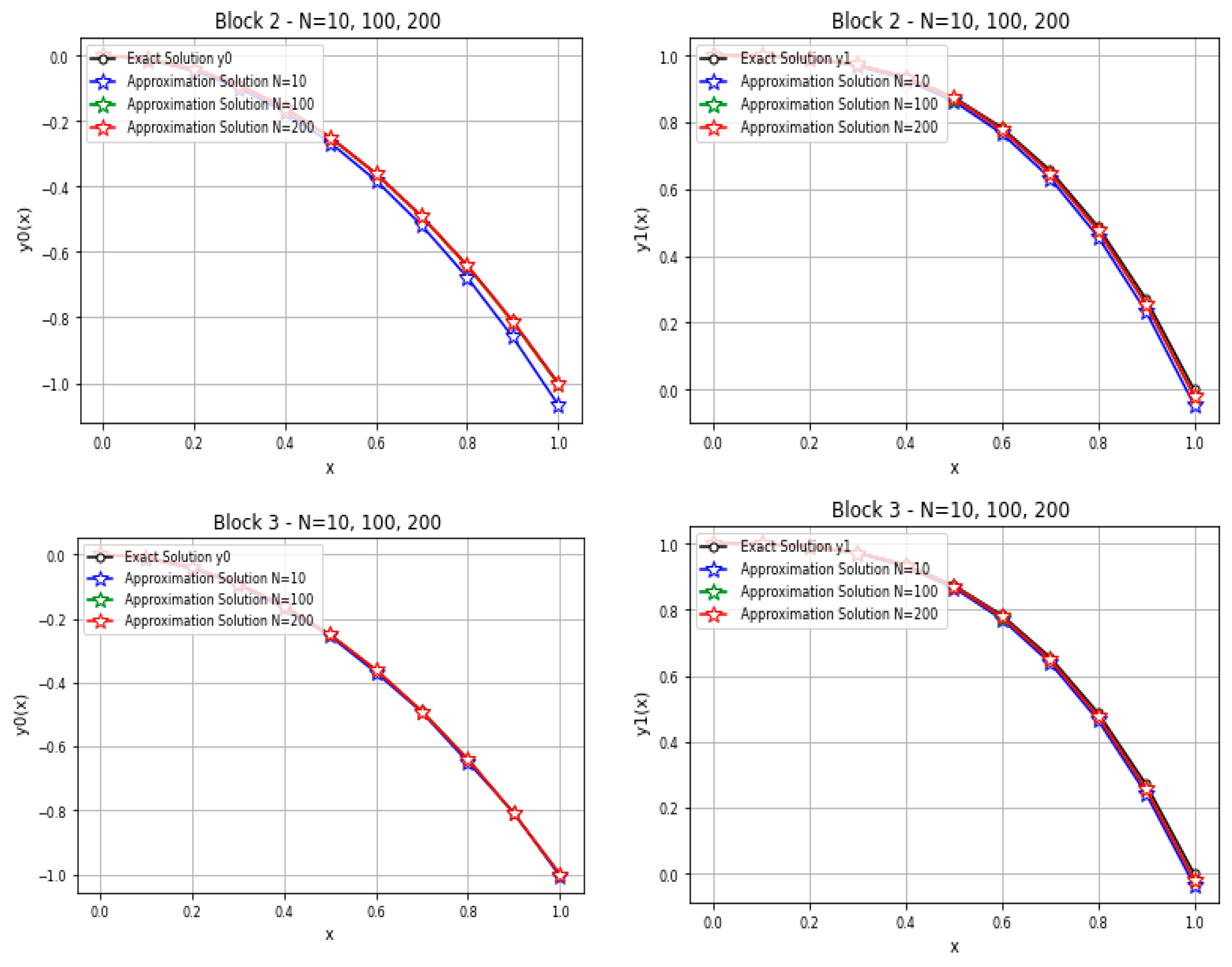
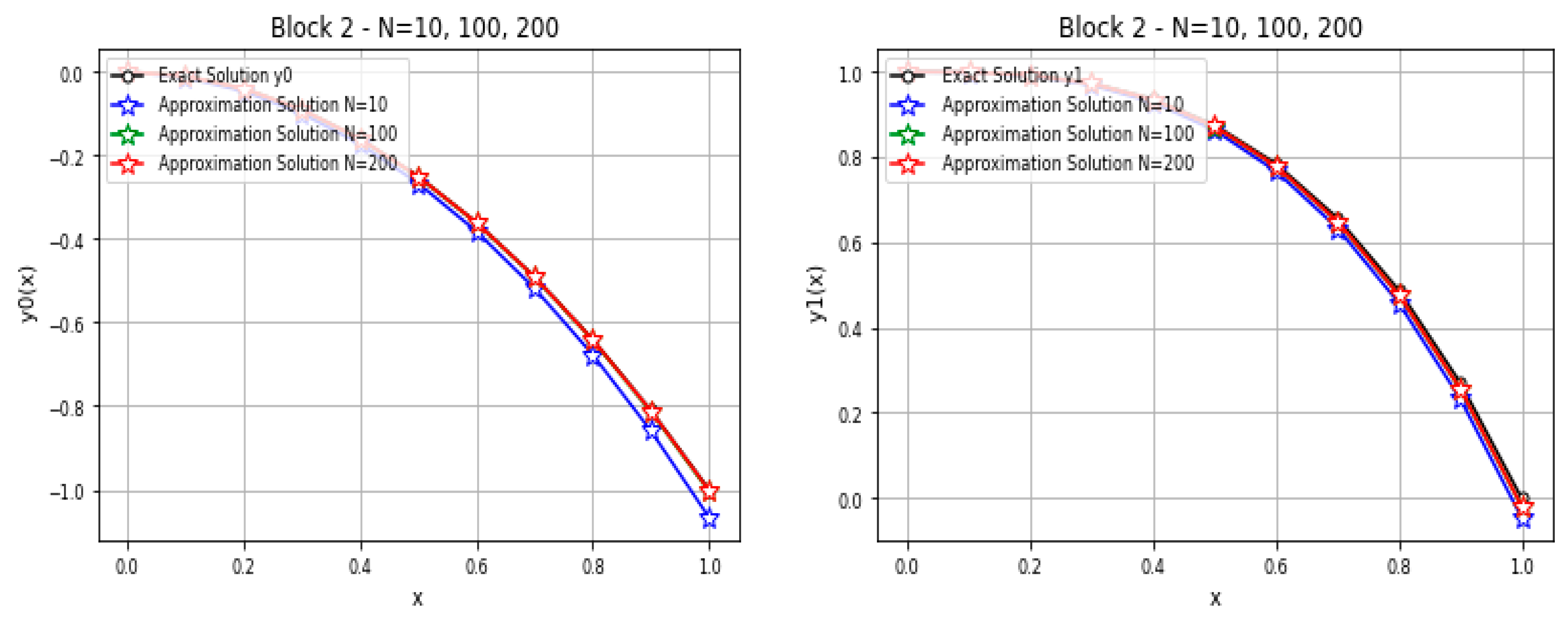
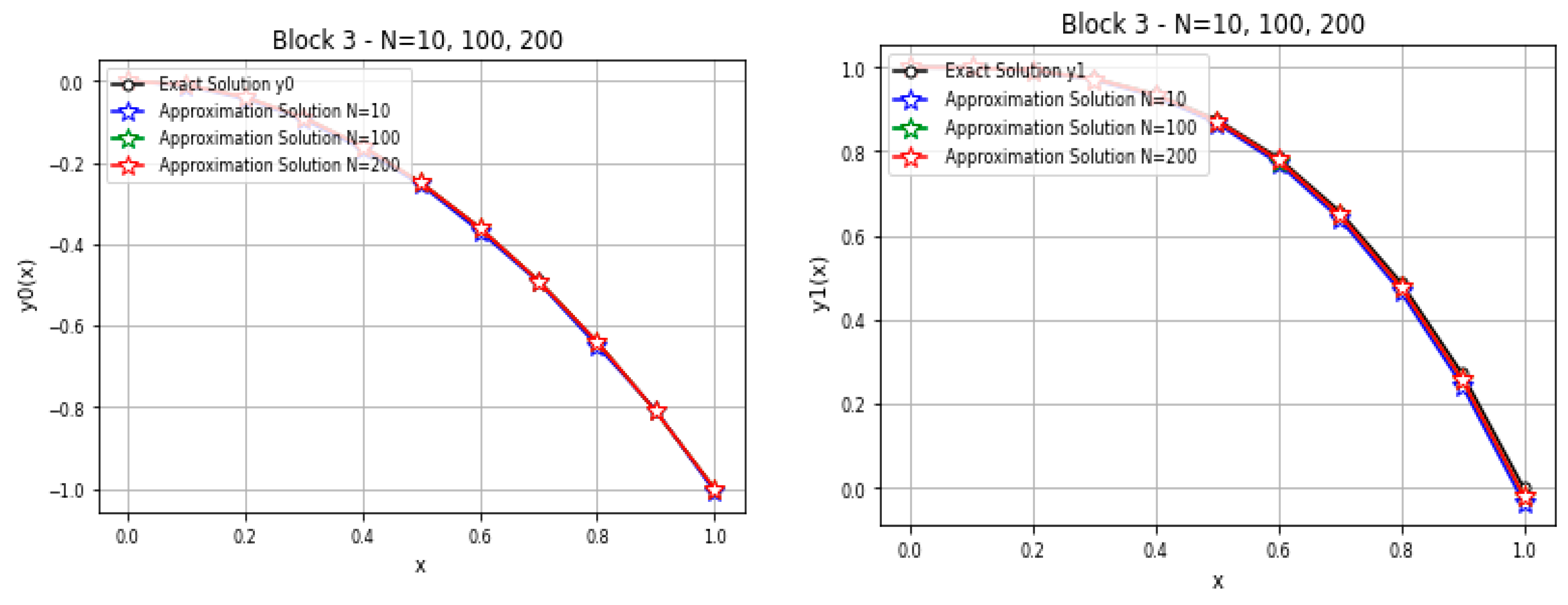
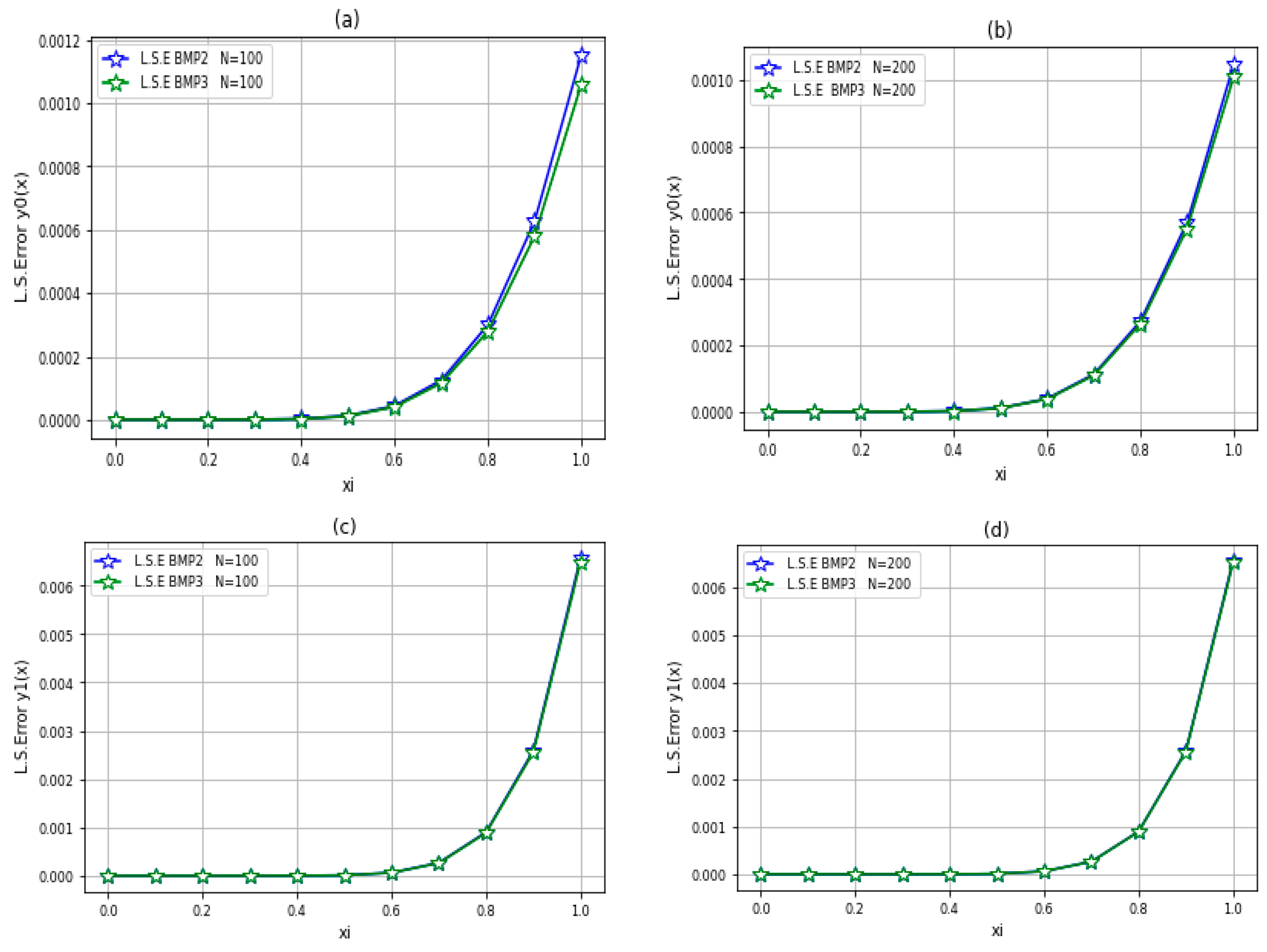
5. Implementation of the Method

In this section, we are demonstrating the simplicity and efficiency of the introduced numerical method by some examples are given for the LSVIFDEs in the Caputo sense for all multi-fractional order $\mathrm{lies} \mathrm{in} \left(0,1\right]$. All results are computed by using of a program written in the Python for algorithms BMP2 and BMP3. The least square error for each problem, denoted by ${(L.S.E)}_y$ and defined by

$${\left(L.S.U\right)}_y=\left[SUM(L.S.Uofall{y_i}^{\prime }s)\right]/m$$

Example 1. 

Consider the following linear system Volterra integro-fractional differential equations with variable coefficients for all fractional orders $\mathrm{lies} \mathrm{in} \left(0,1\right]$:

$$\begin{array}{c}{{}^{c}D}_x^{0.9}{y}_0\left(x\right)+{{}^{c}D}_x^{0.6}{y}_0\left(x\right)+2x{y}_0\left(x\right)\\ =\frac{-2}{\mathsf{\Gamma }\left(2.1\right)}{x}^{1.1}-\frac{2}{\mathsf{\Gamma }\left(2.4\right)}{x}^{1.4}+10e^x\frac{x^{2.7}}{\mathsf{\Gamma }\left(3.7\right)}-{2x}^3+{\int }_0^{x}5e^x{{}^{c}D}_{}^{0.3}{y}_0\left(t\right)dt\end{array}$$

$$\begin{array}{c}{{}^{c}D}_x^{0.8}{y}_1\left(x\right)+x{{}^{c}D}_x^{0.5}{y}_1\left(x\right)\\ =\frac{-6}{\mathsf{\Gamma }\left(3.2\right)}{x}^{2.2}-\frac{6}{\mathsf{\Gamma }\left(3.5\right)}{x}^{3.5}+\frac{6\sin \left(x\right)}{\mathsf{\Gamma }\left(4.2\right)}{x}^{3.2}-\frac{6}{4.2\mathsf{\Gamma }\left(3.2\right)}{x}^{4.2}\\ +{\int }_0^x(\sin \left(x\right)-t){{}^{c}D}_{}^{0.8}{y}_0\left(t\right)dt\end{array}$$

Together with initial conditions: $y_0\left(0\right)=0$ and $y_1\left(0\right)=1$, whereas the exact solutions are $y_0\left(x\right)={-x}^2$ and $y_1\left(x\right)={1-x}^3.$

Take $N=10,h=0.1,x_r=a+rh$; $r=0,1,2,\dots ,N-1$. Here we have the following: ${\mathcal{K}}_0^0\left(x,t\right)=5e^x;{\mathcal{K}}_1^0\left(x,t\right)=0{;\mathcal{K}}_0^1\left(x,t\right)=\left(\sin \left(x\right)-t\right)\mathrm{a}\mathrm{n}\mathrm{d}{\mathcal{K}}_1^1\left(x,t\right)=0.n=2$ and $m=1$ with fractional orders: ${\alpha }_{02}=0.9,{\alpha }_{01}=0.6,{\alpha }_{12}=0.8,{\alpha }_{11}=0.5,{\beta }_{01}=0.3,{\beta }_{10}=0.8$ and ${\alpha }_{00}={\beta }_{00}=0$ with variable coefficients ${\mathcal{P}}_{00}\left(x\right)={\mathcal{P}}_{10}\left(x\right)={\mathcal{P}}_{01}\left(x\right)=1;{\mathcal{P}}_{02}\left(x\right)=2x,{\mathcal{P}}_{11}\left(x\right)=x,{\mathcal{P}}_{12}\left(x\right)=0$. By running the programs, the following obtained all

Table 1. Contains all value of ${\mathcal{H}}_{n,k}^{i,\alpha }\mathrm{a}\mathrm{n}\mathrm{d}{\mathcal{H}}_{m,j}^{i,\beta }$ for the two-block method where $N=10,100\mathrm{a}\mathrm{n}\mathrm{d}200$.

${\mathcal{H}}_{\mathit{n},\mathit{k}}^{\mathit{i},\mathit{\alpha }};{\mathcal{H}}_{\mathit{m},\mathit{j}}^{\mathit{i},\mathit{\beta }}$	$\mathbf{B}\mathbf{M}\mathbf{P}2$ $\mathit{N}=10$	$\mathbf{B}\mathbf{M}\mathbf{P}2$ $\mathit{N}=100$	$\mathbf{B}\mathbf{M}\mathbf{P}2$ $\mathit{N}=200$
${\mathcal{H}}_{2,0}^{0,\mathit{\alpha }}$	$15.58067692$	$123.76171593$	$230.9475281$
${\mathcal{H}}_{2,1}^{0,\mathit{\alpha }}$	$6.80088179$	$27.07479805$	$41.03771995$
${\mathcal{H}}_{2,0}^{1,\mathit{\alpha }}$	$11.96469116$	$75.4920976$	$131.43937618$
${\mathcal{H}}_{2,1}^{1,\mathit{\alpha }}$	$5.04626504$	15.95769122	$22.56758334$
${\mathcal{H}}_{2,2}^{0,\mathit{\alpha }}={\mathcal{H}}_{2,2}^{1,\mathit{\alpha }}$	$1$	$1$	$1$
${\mathcal{H}}_{1,0}^{0,\mathit{\beta }}$	$2.70344634$	$5.39408459$	$6.64089711$
${\mathcal{H}}_{1,0}^{1,\mathit{\beta }}$	$11.96469116$	$75.4920976$	$131.43937618$
${\mathcal{H}}_{1,1}^{0,\mathit{\beta }}={\mathcal{H}}_{1,1}^{1,\mathit{\beta }}$	$1$	$1$	$1$

,

Table 2. Contains all value of ${\mathcal{H}}_{n,k}^{i,\alpha }\mathrm{a}\mathrm{n}\mathrm{d}{\mathcal{H}}_{m,j}^{i,\beta }$ for the three-block method where $N=10,100\mathrm{a}\mathrm{n}\mathrm{d}200$.

${\mathcal{H}}_{\mathit{n},\mathit{k}}^{\mathit{i},\mathit{\alpha }};{\mathcal{H}}_{\mathit{m},\mathit{j}}^{\mathit{i},\mathit{\beta }}$	$\mathbf{B}\mathbf{M}\mathbf{P}3$ $\mathit{N}=10$	$\mathbf{B}\mathbf{M}\mathbf{P}3$ $\mathit{N}=100$	$\mathbf{B}\mathbf{M}\mathbf{P}3$ $\mathit{N}=200$
${\mathcal{H}}_{2,0}^{0,\mathit{\alpha }}$	$22.44235642$	$178.26597355$	$332.65606918$
${\mathcal{H}}_{2,1}^{0,\mathit{\alpha }}$	$8.67401126$	$34.53186079$	$52.34051347$
${\mathcal{H}}_{2,0}^{1,\mathit{\alpha }}$	$16.54910456$	$104.41779068$	$181.80193299$
${\mathcal{H}}_{2,1}^{1,\mathit{\alpha }}$	$6.18038723$	$19.54410048$	$27.63953196$
${\mathcal{H}}_{2,2}^{0,\mathit{\alpha }}={\mathcal{H}}_{2,2}^{1,\mathit{\alpha }}$	$1$	$1$	$1$
${\mathcal{H}}_{1,0}^{0,\mathit{\beta }}$	$3.05312883$	$6.0917929$	$7.4998768$
${\mathcal{H}}_{1,0}^{1,\mathit{\beta }}$	$16.54910456$	104.41779068	$181.80193299$
${\mathcal{H}}_{1,1}^{0,\mathit{\beta }}={\mathcal{H}}_{1,1}^{1,\mathit{\beta }}$	$1$	$1$	$1$

,

Table 3. A comparison between the exact solution and numerical solution using two-block and three-block methods depending on least square error and running time for $N=10$.

	${\mathit{y}}_0\left(\mathit{x}\right)$			${\mathit{y}}_1\left(\mathit{x}\right)$
$\mathit{x}$	$\mathbf{E}\mathbf{x}\mathbf{a}\mathbf{c}\mathbf{t}$	$\mathbf{B}\mathbf{M}\mathbf{P}2$	$\mathbf{B}\mathbf{M}\mathbf{P}3$	$\mathbf{E}\mathbf{x}\mathbf{a}\mathbf{c}\mathbf{t}$	$\mathbf{B}\mathbf{M}\mathbf{P}2$	$\mathbf{B}\mathbf{M}\mathbf{P}3$
$0.0$	$0.00$	$0.0$	$0.0$	$1.000$	$1$	$1$
$0.1$	$-0.01$	$-0.0133399$	$-0.01201728$	$0.999$	$0.9984504$	$0.99866048$
$0.2$	$-0.4$	$-0.04630336074$	$-0.04387683293$	$0.992$	$0.99001318428$	$0.99071904024$
$0.3$	$-0.09$	$-0.09932769925$	$-0.09441522742$	$0.973$	$0.96867129246$	$0.97015110022$
$0.4$	$-0.16$	$-0.17268975073$	$-0.1667659284$	$0.936$	$0.92835775574$	$0.93075651777$
$0.5$	$-0.25$	$-0.26668380513$	$-0.25505162267$	$0.875$	$0.86304032411$	$0.86659591474$
$0.6$	$-0.36$	$-0.38168777473$	$-0.36880182427$	$0.784$	$0.76675844428$	$0.77152149574$
$0.7$	$-0.49$	$-0.51822851730$	$-0.49322309007$	$0.657$	$0.63362356671$	$0.63978482496$
$0.8$	$-0.64$	$-0.67707434414$	$-0.64932899451$	$0.488$	$0.45778737039$	$0.46536622778$
$0.9$	$-0.81$	$-0.85938104583$	$-0.80729230200$	$0.271$	$0.23338351416$	$0.24244697072$
$1.0$	$-1$	$-1.06693235396$	$-1.00653583547$	$0.000$	$-0.0455495788$	$-0.0349831482$
L.S.E ${\mathit{y}}_0\left(\mathit{x}\right)$		$1.0137416\times {10}^{-2}$	$3.3482949\times {10}^{-4}$	L.S.E $y_1\left(x\right)$	$5.47072095\times {10}^{-3}$	$3.11145422\times {10}^{-3}$
$\mathbf{R}.\mathbf{T}\mathbf{i}\mathbf{m}\mathbf{e}/\mathbf{S}$		$BMP2=0.046821117$		$BMP3=0.250024557$

and

Table 4. The mean least square errors and running times for using two-block and three-block methods with various choices of step size $h=(b-a)/N$.

Block-by-Block Method	$\mathit{N}=10$	$\mathbf{R}.\mathbf{T}\mathbf{i}\mathbf{m}\mathbf{e}/\mathbf{S}$	$\mathit{N}=100$	$\mathbf{R}.\mathbf{T}\mathbf{i}\mathbf{m}\mathbf{e}/\mathbf{S}$	$\mathit{N}=200$	$\mathbf{R}.\mathbf{T}\mathbf{i}\mathbf{m}\mathbf{e}/\mathbf{S}$
	${\left(\mathbf{L}.\mathbf{S}.\mathbf{E}\right)}_{\mathit{y}}$		${\left(\mathbf{L}.\mathbf{S}.\mathbf{E}\right)}_{\mathit{y}}$		${\left(\mathbf{L}.\mathbf{S}.\mathbf{E}\right)}_{\mathit{y}}$
$\mathbf{B}\mathbf{M}\mathbf{P}2$	$7.80406839$ $\times {10}^{-3}$	$0.046821117$	$4.7014974$ $\times {10}^{-4}$	$25.2331798$	$3.9918725$ $\times {10}^{-4}$	$185.8057982$
$\mathbf{B}\mathbf{M}\mathbf{P}3$	$1.72314185$ $\times {10}^{-3}$	$0.250024557$	$4.0882842$ $\times {10}^{-4}$	$168.7220046$	$3.7973148$ $\times {10}^{-4}$	$1419.887972$

.

We completed all the steps in the algorithms BMP2 and BMP3. Table 3 presents a comparison between the exact solution and the block-by-block methods. The numerical solution of the forward finite difference techniques via block-by-block methods (a new technique) for $y_0\left(t\right)$ and $y_1\left(t\right)$ depending on the least square error, see Table 3 and Table 4 and Figure 1.

Example 2. 

Consider the following LSVIFDEs with variable coefficients for all fractional orders lies in $\left(0,1\right]$, given by

$${{}^{c}D}_x^{0.7}{y}_0\left(x\right)+{{}^{c}D}_x^{0.5}{y}_0\left(x\right)-2y_0\left(x\right)=f_0\left(x\right)+{\int }_0^x\left[x{{}^{c}D}_t^{0.3}{y}_0\left(t\right)+(x-t)y_1\left(t\right)\right]dt$$

$${{}^{c}D}_x^{0.6}{y}_1\left(x\right)+e^x{{}^{c}D}_x^{0.4}{y}_1\left(x\right)+x{y}_1\left(x\right)=f_1\left(x\right)+{\int }_0^x\left[(x-2t){{}^{c}D}_t^{0.8}{y}_0\left(t\right)\right]dt$$

where

$$f_0\left(x\right)=\frac{24}{\mathsf{\Gamma }\left(4.3\right)}{x}^{3.3}+\frac{24}{\mathsf{\Gamma }\left(4.5\right)}{x}^{3.5}-\frac{24}{\mathsf{\Gamma }\left(5.7\right)}{x}^{5.7}-\frac{1}{30}{x}^6-2x^4$$

$$\begin{gathered} f_1\left(x\right)=\frac{1}{\mathsf{\Gamma }\left(1.4\right)}{x}^{0.4}-\frac{2}{\mathsf{\Gamma }\left(2.4\right)}{x}^{1.4}+\frac{e^x}{\mathsf{\Gamma }\left(1.6\right)}{x}^{0.6}-\frac{2e^x}{\mathsf{\Gamma }\left(2.6\right)}{x}^{1.6}-\frac{1}{\mathsf{\Gamma }\left(2.2\right)}{x}^{2.2}+\frac{2}{\mathsf{\Gamma }\left(3.2\right)}{x}^{3.2} \\ +\frac{2}{2.2\mathsf{\Gamma }\left(1.2\right)}{x}^{2.2}-\frac{4}{3.2\mathsf{\Gamma }\left(2.2\right)}{x}^{3.2}+x^2-x^3 \end{gathered}$$

With initial conditions $y_0\left(0\right)=y_1\left(0\right)=0$, whereas the exact solutions are $y_0\left(x\right)=x^4$; $y_1\left(x\right)=x\left(1-x\right).$

Because we have ${\mathcal{K}}_0^0\left(x,t\right)=x;{\mathcal{K}}_1^0\left(x,t\right)=x-t{;\mathcal{K}}_0^1\left(x,t\right)=x-2t\mathrm{a}\mathrm{n}\mathrm{d}{\mathcal{K}}_1^1\left(x,t\right)=0$ with variable coefficients ${{\mathcal{P}}_{00}\left(x\right)=\mathcal{P}}_{01}\left(x\right)={\mathcal{P}}_{10}\left(x\right)=1;{\mathcal{P}}_{02}\left(x\right)=-2,{\mathcal{P}}_{11}\left(x\right)=e^x\mathrm{a}\mathrm{n}\mathrm{d}{\mathcal{P}}_{12}\left(x\right)=x.$

We completed all the steps in the algorithms BMP2 and BMP3. After using the information’s in

Table 5. Contains all value of ${\mathcal{H}}_{n,k}^{i,\alpha }\mathrm{a}\mathrm{n}\mathrm{d}{\mathcal{H}}_{m,j}^{i,\beta }$ for the two-block method where $N=10,100\mathrm{a}\mathrm{n}\mathrm{d}200$.

${\mathcal{H}}_{\mathit{n},\mathit{k}}^{\mathit{i},\mathit{\alpha }};{\mathcal{H}}_{\mathit{m},\mathit{j}}^{\mathit{i},\mathit{\beta }}$	$\mathbf{B}\mathbf{M}\mathbf{P}2$ $\mathit{N}=10$	$\mathbf{B}\mathbf{M}\mathbf{P}2$ $\mathit{N}=100$	$\mathbf{B}\mathbf{M}\mathbf{P}2$ $\mathit{N}=200$
${\mathcal{H}}_{2,0}^{0,\mathit{\alpha }}$	$9.0719515$	$45.46746277$	$73.86211117$
${\mathcal{H}}_{2,1}^{0,\mathit{\alpha }}$	$5.04626504$	$15.95769122$	$22.56758334$
${\mathcal{H}}_{2,0}^{1,\mathit{\alpha }}$	$6.80088179$	$27.07479805$	$41.03771995$
${\mathcal{H}}_{2,1}^{1,\mathit{\alpha }}$	$3.70945392$	$9.31772698$	$12.29481446$
${\mathcal{H}}_{2,2}^{0,\mathit{\alpha }}={\mathcal{H}}_{2,2}^{1,\mathit{\alpha }}$	$1$	$1$	$1$
${\mathcal{H}}_{1,0}^{0,\mathit{\beta }}$	$2.70344634$	$5.39408459$	$6.64089711$
${\mathcal{H}}_{1,0}^{1,\mathit{\beta }}$	$11.96469116$	$75.4920976$	$131.43937618$
${\mathcal{H}}_{1,1}^{0,\mathit{\beta }}={\mathcal{H}}_{1,1}^{1,\mathit{\beta }}$	$1$	$1$	$1$

and

Table 6. Contains all value of ${\mathcal{H}}_{n,k}^{i,\alpha }\mathrm{a}\mathrm{n}\mathrm{d}{\mathcal{H}}_{m,j}^{i,\beta }$ for the three-block method where $N=10,100\mathrm{a}\mathrm{n}\mathrm{d}200$.

${\mathcal{H}}_{\mathit{n},\mathit{k}}^{\mathit{i},\mathit{\alpha }};{\mathcal{H}}_{\mathit{m},\mathit{j}}^{\mathit{i},\mathit{\beta }}$	$\mathbf{B}\mathbf{M}\mathbf{P}3$ $\mathit{N}=10$	$\mathbf{B}\mathbf{M}\mathbf{P}3$ $\mathit{N}=100$	$\mathbf{B}\mathbf{M}\mathbf{P}3$ $\mathit{N}=200$
${\mathcal{H}}_{2,0}^{0,\mathit{\alpha }}$	$12.04937723$	$60.38994042$	$98.10374765$
${\mathcal{H}}_{2,1}^{0,\mathit{\alpha }}$	$6.18038723$	$19.54410048$	$27.63953196$
${\mathcal{H}}_{2,0}^{1,\mathit{\alpha }}$	$8.67401126$	$34.53186079$	$52.34051347$
${\mathcal{H}}_{2,1}^{1,\mathit{\alpha }}$	$4.36261094$	$10.95838323$	$14.45967337$
${\mathcal{H}}_{2,2}^{0,\mathit{\alpha }}={\mathcal{H}}_{2,2}^{1,\mathit{\alpha }}$	$1$	$1$	$1$
${\mathcal{H}}_{1,0}^{0,\mathit{\beta }}$	$3.05312883$	$6.0917929$	$7.4998768$
${\mathcal{H}}_{1,0}^{1,\mathit{\beta }}$	$16.54910456$	$104.41779068$	$181.80193299$
${\mathcal{H}}_{1,1}^{0,\mathit{\beta }}={\mathcal{H}}_{1,1}^{1,\mathit{\beta }}$	$1$	$1$	$1$

we obtain

Table 7. The comparison between the exact solution and numerical solution using two-block and three-block methods depending on least square error and running time for $N=10$.

	${\mathit{y}}_0\left(\mathit{x}\right)$			${\mathit{y}}_1\left(\mathit{x}\right)$
$\mathit{x}$	$\mathbf{E}\mathbf{x}\mathbf{a}\mathbf{c}\mathbf{t}$	$\mathbf{B}\mathbf{M}\mathbf{P}2$	$\mathbf{B}\mathbf{M}\mathbf{P}3$	$\mathbf{E}\mathbf{x}\mathbf{a}\mathbf{c}\mathbf{t}$	$\mathbf{B}\mathbf{M}\mathbf{P}2$	$\mathbf{B}\mathbf{M}\mathbf{P}3$
$0.0$	$0.0000$	$0.0$	$0.0$	$0.00$	$0.0$	$0.0$
$0.1$	$0.0001$	$0.00017600419$	$0.00011142044$	$0.09$	$0.0885394561$	$0.08999196501$
$0.2$	$0.0016$	$0.00218275302$	$0.00173099784$	$0.16$	$0.15778964412$	$0.16003625270$
$0.3$	$0.0081$	$0.01008512719$	$0.00865379048$	$0.21$	$0.20706630902$	$0.20987638340$
$0.4$	$0.0256$	$0.03041946795$	$0.02713854520$	$0.24$	$0.23578330581$	$0.23903787881$
$0.5$	$0.0625$	$0.07218455507$	$0.06587879423$	$0.25$	$0.24316336722$	$0.24679896667$
$0.6$	$0.1296$	$0.14682235856$	$0.13596823567$	$0.24$	$0.22817032464$	$0.23216246675$
$0.7$	$0.2401$	$0.26818749436$	$0.25085389684$	$0.21$	$0.18947806296$	$0.19383675025$
$0.8$	$0.4096$	$0.45250140750$	$0.42627111448$	$0.16$	$0.12546287371$	$0.13023394799$
$0.9$	$0.6561$	$0.71828591453$	$0.68015349552$	$0.09$	$0.03421792128$	$0.03948863309$
$1.0$	$1.0000$	$1.08626922053$	$1.03250943177$	$0.00$	$-0.08641136656$	$-0.08050292670$
L.S.E ${\mathit{y}}_0\left(\mathit{x}\right)$		$1.435681810$ $\times {10}^{-2}$	$7.16765525$ $\times {10}^{-3}$	L.S.E $y_1\left(x\right)$	$1.241261424$ $\times {10}^{-2}$	$1.040173476$ $\times {10}^{-2}$
$\mathbf{R}.\mathbf{T}\mathbf{i}\mathbf{m}\mathbf{e}/\mathbf{S}$		$\mathrm{B}\mathrm{M}\mathrm{P}2=0.046799659$		$\mathrm{B}\mathrm{M}\mathrm{P}3$ = 1.720833539

which presents a comparison between the exact solution and the block-by-block methods.

The numerical solution of the forward finite difference techniques via block-by-block methods (a new technique) for $y_0\left(t\right)$ and $y_1\left(t\right)$ depending on the least square error, see Table 7 and

Table 8. The mean least square errors and running times for two-block and three-block methods with various choices of step size $h$.

Block-by-Block Method	$\mathit{N}=10$	$\mathbf{R}.\mathbf{T}\mathbf{i}\mathbf{m}\mathbf{e}/\mathbf{S}$	$\mathit{N}=100$	$\mathbf{R}.\mathbf{T}\mathbf{i}\mathbf{m}\mathbf{e}/\mathbf{S}$	$\mathit{N}=200$	$\mathbf{R}.\mathbf{T}\mathbf{i}\mathbf{m}\mathbf{e}/\mathbf{S}$
	${\left(\mathbf{L}.\mathbf{S}.\mathbf{E}\right)}_{\mathit{y}}$		${\left(\mathbf{L}.\mathbf{S}.\mathbf{E}\right)}_{\mathit{y}}$		${\left(\mathbf{L}.\mathbf{S}.\mathbf{E}\right)}_{\mathit{y}}$
$\mathbf{B}\mathbf{M}\mathbf{P}2$	$1.338471617$ $\times {10}^{-2}$	$0.046799659$	$6.32473407$ $\times {10}^{-3}$	$25.64327144$	$6.20364139$ $\times {10}^{-3}$	$194.53524470$
$\mathbf{B}\mathbf{M}\mathbf{P}3$	$8.784695$ $\times {10}^{-3}$	$1.720833539$	$6.16783582$ $\times {10}^{-3}$	$195.5688905$	$6.13445657$ $\times {10}^{-3}$	$1445.007089$

also Figure 2 and Figure 3.

6. Discussion

We present two numerical approaches for solving the linear system Volterra Integro Fractional Differential Equation (LSVIFDEs) of Caputo derivative sense in the range of $\left(0,1\right]$ with variable coefficients. In addition, we apply two numerical algorithms to solve the LSVIFDEs using two-block (BMP2) and two-block (BMP3) methods with the aid of forward finite difference scheme for a Caputo derivative. For each algorithm, a computer program was written. Moreover, we display the comparison of computing accuracy and speed, as well as the least square error and running times in Table 3, Table 4, Table 7 and Table 8. We conclude:

• The numerical experiments have shown that the three-block method (BMP3) gives better accuracy than the two-block method (BMP2);
• Where $N$ are sufficiently large number, the error to be minimizes and the results are approached to the exact solution;
• The two-block method (BMP2) is faster, and lower in accuracy, than the three-block method (BMP3).

References

1. Podldubny, I. Fractional Differential Equation; Academic Press: San Diego, CA, USA, 1999. [Google Scholar]
2. Kilbas, A.A.; Srivastava, H.M.; Trujillo, J.J. Theory and Applications of Fractional Differential Equations; Elsevier: Amsterdam, The Netherlands, 2006. [Google Scholar]
3. Sabatier, J.; Agrawal, O.P.; Machado, J.A.T. Advances in Fractional Calculus: Theoretical Developments and Applications in Physics and Engineering; Beijing World Publishing Corporation: Beijing, China, 2014. [Google Scholar]
4. Miller, K.S.; Ross, B. An Introduction to the Fractional Calculus and Fractional Differential Equations; John Wiley & Sons: New York, NY, USA, 1993. [Google Scholar]
5. Podlubny, I. Geometric and Physical Interpretation of Fractional Integral and Fractional Differentiation. J. Fract. Calc. Appl. Anal. 2002, 5, 367–386. [Google Scholar]
6. Erturk, V.S.; Kumar, P. Solution of a COVID-19 model via new generalized Caputo-type fractional derivatives. Chaos Solitons Fractals 2020, 139, 110280. [Google Scholar] [CrossRef] [PubMed]
7. Iomin, A. Fox H-Functions in Self-Consistent Description of a Free-Electron Laser. Fractal Fract. 2021, 5, 263. [Google Scholar] [CrossRef]
8. Turab, A.; Rosli, N. Study of Fractional Differential Equations Emerging in the Theory of Chemical Graphs: A Robust Approach. Mathematics 2022, 10, 4222. [Google Scholar] [CrossRef]
9. Turab, A.; Mitrović, Z.D.; Savić, A. Existence of solutions for a class of nonlinear boundary value problems on the hexasilinane graph. Adv. Differ. Equ. 2021, 494. [Google Scholar] [CrossRef]
10. Liu, J.-G.; Yang, X.-J.; Geng, L.-L.; Yu, X.-J. On fractional symmetry group scheme to the higher-dimensional space and time fractional dissipative Burger’s equation. Int. J. Geom. Methods Mod. Phys. 2022, 19, 2250173. [Google Scholar] [CrossRef]
11. Baleanu, D.; Jajarmi, A.; Asad, J.H.; Blaszczyk, T. The Motion of a Bead Sliding on a Wire in Fractional Sense. Acta Phys. Pol. A 2017, 131, 1561–1564. [Google Scholar] [CrossRef]
12. Baleanu, D.; Jajarmi, A.; Mohammadi, H.; Rezapour, S. A new study on the mathematical modelling of human liver with Caputo-Fabrizio fractional derivative. Chaos Soliton. Fractals 2020, 134, 109705. [Google Scholar] [CrossRef]
13. Hesameddini, E.; Shahbazi, M. Hybrid Bernstein block–pulse functions for solving system of fractional integro-differential equations. Int. J. Comput. Math. 2018, 95, 2287–2307. [Google Scholar] [CrossRef]
14. Ahmed, S.S. Solving a System of Fractional-Order Volterra Integro-Differential Equations Based on the Explicit Finite Difference Approximation via the Trapezoidal Method with Error Analysis. Symmetry 2022, 14, 575. [Google Scholar] [CrossRef]
15. Linz, P. Analytical and Numerical Methods for Volterra Integral Equations; SIAM: Philadelphia, PA, USA, 1985. [Google Scholar]
16. Weilbeer, M. Efficient Numerical Methods for Fractional Differential Equations and Their Analytical Background; US Army Medical Research and Material Command: Fort Detrick, MD, USA, 2005.
17. Hosseini, M.M. Adomian decomposition method for solution of nonlinear differential algebraic equations. Appl. Math. Comput. 2006, 181, 1737–1744. [Google Scholar] [CrossRef]
18. Odibat, Z.; Momani, S.; Xu, H. A reliable algorithm of homotopy analysis method for solving nonlinear fractional differential equations. Appl. Math. Model. 2010, 34, 593–600. [Google Scholar] [CrossRef]
19. Rawashdeh, E.A. Numerical solution of fractional integro-differential equations by collocation method. Appl. Math. Comput. 2006, 176, 1–6. [Google Scholar] [CrossRef]
20. Doha, E.H.; Bhrawy, A.H.; Ezz-Eldien, S.S. A new Jacobi operational matrix: An application for solving fractional differential equations. Appl. Math. Model. 2012, 36, 4931–4943. [Google Scholar] [CrossRef]
21. Mustafa, M.; Ibrahem, T.A.L. Numerical Solution of Volterra Integral Equations with Delay Using Block Method. Al-Fatih J. 2008, 4, 42–51. [Google Scholar]
22. Katani, R.; Shamorad, S. Block-by-Block method for the system of nonlinear Volterra integral equations. Appl. Math. Model. 2010, 34, 400–406. [Google Scholar] [CrossRef]
23. Mohamad, M.B. Numerical Treatment for Solving Linear Fractional-Order Volterra Integro-Differential Equations with Constant Time-Delay of Retarded. Master’s Thesis, University of Sulaimani, Sulaimani, Iraq, 2016. [Google Scholar]
24. Saleh, A.J. Numerical Solutions of Systems of Nonlinear Volterra Integro Differential Equations [VIDEs] Using Block Method. J. Glob. Sci. Res. Appl. Math. Stat. 2022, 7, 2452–2463. [Google Scholar]
25. Ahmed, S.S.; Salh, S.A.H. Numerical Treatment of the most General Linear Volterra Integro-Fractional Differential Equations with Caputo Derivatives by Quadrature Methods. J. Math. Comput. Sci. 2012, 2, 1293–1311. [Google Scholar]
26. Salih, S.A.H. Some Computational Methods for Solving Linear Volterra Integro-Fractional Differential Equations. Master’s Thesis, University of Sulaimani, Sulaimani, Iraq, 2011. [Google Scholar]
27. Ahmed, S.S. On System of Linear Volterra Integro-Fractional Differential Equations. Ph.D. Thesis, Sulaimani University, Sulaimani, Iraq, 2009. [Google Scholar]
28. Chenecy, W.; Kincaid, D. Numerical Mathematics and Computation, 4th ed.; ITP An international Thomson Publishing Company: Kyoto, Japan, 1999. [Google Scholar]
Figure 1. The numerical approximation of y 0 t , y 1 t by BMP2 and BMP3 with exact solution of Example 1.
Symmetry 15 00607 g001
Figure 2. The numerical approximation of y 0 t , y 1 t by BMP2 and BMP3 with exact solution of Example 2.
Symmetry 15 00607 g002aSymmetry 15 00607 g002b
Figure 3. (a) Least square error comparation of BMP2 and BMP3 for y 0 x   a n d   N = 100 . (b) Least square error comparation of BMP2 and BMP3 for y 0 x   a n d   N = 200 . (c) Least square error comparation of BMP2 and BMP3 for y 1 x   a n d   N = 100 . (d) Least square error comparation of BMP2 and BMP3 for y 1 x   a n d   N = 200 .
Symmetry 15 00607 g003