Channel Fading Characteristics of Hyperloop Scenarios Based on Ray-Tracing Model

Abstract

Hyperloop is envisioned as the next generation of railway transportation mode, which can proceed at a speed of more than 1000 km/h. The safe operation of the Hyperloop depends heavily on the support of a stable communication system. In this paper, we propose a 3D channel model in vacuum tube scenarios based on the ray-tracing method. The reflection paths and line of sight (LoS) paths are considered. We derive the channel transfer function (CTF) expression for each multipath, and then the channel impulse response (CIR) is obtained. On this basis, the large-scale and small-scale channel characteristics, including path loss, shadow fading, correlation coefficient, delay spread, and angular spread, are investigated and analyzed. Simulation results show that the proposed channel model can characterize the wireless channel in the Hyperloop scenarios in detail, and the results maintain a high level of symmetry between the range of 0–250 m and 250–500 m. The relevant research results will contribute to the design of future Hyperloop wireless communication systems.

1. Introduction

With the rapid development of the national economy, railway transportation has made remarkable achievements [1]. High velocity is always the eternal pursuit of mankind. Nowadays, as a novel land transport mode for passengers and freight, Hyperloop has gradually entered the public’s vision [2]. Hyperloop exceeds the limitation of traditional wheel-rail-based high-speed transportation, including mechanical friction, air resistance, and noise [3]. It can proceed at a speed of more than 1000 km/h in the low-pressure pipeline close to the vacuum tube environment regardless of all-weather conditions [4].

As early as 1904, American scholar Robert Goddard first proposed the idea of vacuum pipeline transportation [5]. In recent years, Elon Musk has enriched the concept of vacuum transportation and proposed the ultra-high-speed railway in 2013 [6]. Currently, many countries in the world are stepping up the development of maglev trains. Japan is building a commercial operation line for cryogenic superconducting maglev vehicles, and the United States is developing a super high-speed railway with a speed of 1000 km/h [7]. Meanwhile, China is also actively carrying out relevant works. Southwest Jiaotong University launched a 1500 km/h vacuum tube and a relevant maglev project in 2020 [8]. The Aviation Industry Corporation of China and Shanxi province jointly built a laboratory of high-speed flying train [9], and the first test of the high-speed flying train system was successfully conducted on 15 October 2022 [10]. Meanwhile, the Boring Company, a tunnel excavation company owned by Elon Musk, announced that it would launch the test of the full-size Hyperloop project [11].

From the above research, we can see that the research on Hyperloop at home and abroad has become more and more enthusiastic. Nevertheless, they mainly focus on the vacuum tube equipmentsand maglev systems such as the vacuum tube structure, magnetic suspension mode, etc. It is noteworthy that the train-to-ground communication system is of vital importance to the safe and reliable operation of the train. Compared with the traditional wheel-based high-speed railway (HSR), the Hyperloop owns two unique features, i.e., the ultra-high-speed over 1000 km/h and the metal-confined narrow vacuum tube environment, which leads to severe Doppler effect and frequent handover. For the Doppler effect, the authors in [12] improved the existing standard 4G/5G mobile communication system, the threshold of frequency offset correction algorithm was increased by increasing the subcarrier spacing so that the receiving end can receive the signal correctly, thereby suppressing the Doppler effect in an ultra-high-speed mobile environment. As for the frequent handover, the authors in [13] proposed a fast predictive handover algorithm based on a distributed antenna system (DAS) along with the two-hop architecture to reduce the handover latency and handover command failure probability. At present, the 5G-R network can possibly meet the requirements of high throughput, high reliability, and low latency for smart HSR communications [14]. While the maximum supporting mobile speed of 5G is 500 km/h [15], failing to support vacuum tube communication. It should be noted that the design of a wireless communication system is inseparable from the channel characteristics. In addition, the wireless channel in vacuum tube scenarios is quite different from that in HSR scenarios. Therefore, it is necessary to understand the wireless channel characteristics in the vacuum tube scenario.

Common channel modeling methods mainly include the propagation-graph channel model, geometry-based stochastic model (GBSM), and ray-tracing (RT) method. Some published works like [16] proposed a propagation-graph channel model and analyzed the corresponding position-based wireless channel characteristics. In [17,18], a non-stationary 3-dimensional (3-D) GBSM vehicle-to-vehicle channel model is proposed in the tunnel environment based on massive multiple-input multiple-output (MIMO) antenna arrays, which is similar to the vacuum tube scenario except for the speed. In [19], the authors analyzed the channel characteristics of the ultra-high-speed train (UHST) channels in vacuum tube scenarios based on 3-D non-stationary GBSM. The authors in [20] analyzed the effective scatterers for the Hyperloop train-to-ground wireless communication based on a novel 3-D non-stationary geometry-based deterministic model (GBDM). Moreover, ray tracing is a deterministic method and is widely used due to its high accuracy, especially considering that electronic wave exhibits an evident mechanism of reflection at high-frequency bands. Numerous works have utilized this method to analyze different scenarios, like the works on vehicle-to-infrastructure (V2I) and vehicle-to-vehicle (V2V) scenarios in [21,22] and the works on the intra-wagon environment for 5G between 25 GHz and 40 GHz in [23].

The above research efforts are mainly focused on small-scale fading characteristics. However, large-scale fading characteristics also have a significant impact on the wireless coverage of train communication in the vacuum tube scenario, which is of great significance to network design and interference analysis. Therefore, we mainly aim to simultaneously study the large-scale fading and small-scale fading characteristics of Hyperloops in this paper. The research of channel characteristics in vacuum tube scenarios is of great significance for the future train-to-ground communication system design, including the base station deployment, the antenna design, and so on. In this paper, our main contributions are as follows:

(i)

A 3D ray-tracing model for Hyperloop in vacuum tube scenarios is constructed in this paper. The reflection paths and line of sight (LoS) path are considered.

(ii)

Based on the proposed model, the channel impulse response (CIR) is obtained. Then the large-scale fading and small-scale fading characteristics, including path loss, shadow fading, correlation coefficient, delay spread, and angular spread, are investigated and analyzed.

The remainder of this paper is organized as follows. In Section 2, we introduce the proposed ray-tracing channel model method for Hyperloop communications. Section 3 introduces the simulation setting, and the corresponding simulation results are shown in Section 4. Finally, Section 5 draws the relevant conclusions.

2. System Model

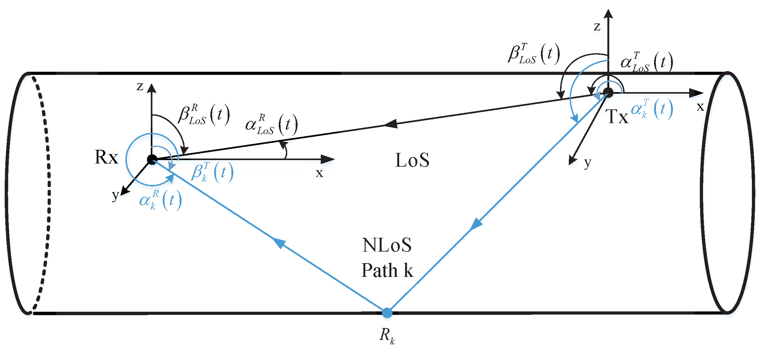
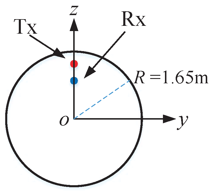
To better illustrate the Hyperloop communication model, we establish a downlink Hyperloop communication scenario in a vacuum tube as shown in Figure 1. The Hyperloop train runs along the speed direction vector $\overline{v}$ in a vacuum tube with a radius of R. The transmitter (Tx) of the communication system is fixed on the top of the tube. The wireless signal is transmitted from the Tx to the receiver (Rx) fixed on the top of the train. Since the metal inner tube surface contributes to rich reflection and the scattering components are few, we will consider the influence of both the LoS component and the reflection components to generate the CIR. The sketch map of two kinds of paths is shown in Figure 1. For the LoS component and non-line of sight (NLoS) components, i.e., the reflection components, we use the azimuth angles of departure (AAoDs), elevation angles of departure (EAoDs), azimuth angles of arrival (AAoAs), and elevation angles of arrival (EAoAs) to describe them. To facilitate further descriptions, we further summarize them in

Table 1. Parameters definitions.

Parameters	Definitions
$A_m^T$,$A_n^R$	positions of m-th Tx and n-th Rx
${\alpha }_{LoS}^T\left(t\right)$, ${\beta }_{LoS}^T\left(t\right)$	azimuth and elevation departure angles of the LoS path
${\alpha }_{LoS}^R\left(t\right)$, ${\beta }_{LoS}^R\left(t\right)$	azimuth and elevation arrival angles of the LoS path
${\alpha }_k^T\left(t\right)$, ${\beta }_k^T\left(t\right)$	azimuth and elevation departure angles of the k-th NLoS path
${\alpha }_k^R\left(t\right)$, ${\beta }_k^R\left(t\right)$	azimuth and elevation arrival angles of the k-th NLoS path
$D_{m,n}^{LoS}\left(t\right)$	path distance of the LoS component
$D_{m,k}^{NLoS}\left(t\right)$	path distance of the NLoS component
from Tx to reflection point $r_k$
$D_{k,n}^{NLoS}\left(t\right)$	path distance of the NLoS component
from reflection point to $r_k$

.

Considering the LoS and NLoS components, the CIR in the vacuum tube scenario can be expressed as

$$h_{m,n}\left(t\right)=h_{m,n}^{LoS}\left(t\right)+h_{m,n}^{NLoS}\left(t\right),$$

(1)

where $h_{m,n}^{LoS}\left(t\right)$ is the CIR of the LoS component from the m-th Tx antenna ($T_m$) to the n-th Rx antenna ($R_n$), and $h_{m,n}^{NLoS}\left(t\right)$ is the CIR of the NLoS component, which refers to reflection components in this paper.

First, we will derive the CIR of the LoS path. Considering the transceiver antennas are omnidirectional, the CIR of link $T_m$-$R_n$ can be expressed as

$$h_{m,n}^{LoS}\left(t\right)=∥h_{m,n}^{LoS}\left(t\right)∥·e^{j\left(2\pi {\lambda }^{-1}{D}_{m,n}^{{}^{LoS}}+{\eta }^{LoS}\right)}·e^{j2\pi {\lambda }^{-1}{\overline{r}}_m·{\overline{\varphi }}_{LoS}^T}·e^{j2\pi {\lambda }^{-1}{\overline{r}}_n·{\overline{\varphi }}_{LoS}^R}·e^{j2\pi f_d^{L\mathrm{o}S}t},$$

(2)

where $∥h_{m,n}^{LoS}\left(t\right)∥$ is the corresponding path gain, $D_{m,n}^{LoS}\left(t\right)$ is the path distance from the center of the Tx array to the center of the Rx array. ${\eta }^{LoS}$ is the initial phase of LoS path and $\lambda$ is the wavelength. ${\overline{r}}_m$ and ${\overline{r}}_n$ are the coordinates of the m-th antenna element in the Tx antenna array and the n-th antenna element in the Rx antenna array, respectively. According to the Friis equation [24], the gain of the LoS path is

$$∥h_{m,n}^{LoS}\left(t\right)∥=\frac{\lambda }{4\pi D_{m,n}^{LoS}\left(t\right)}.$$

(3)

In Equation (2), ${\overline{\varphi }}_{LoS}^T$ is the unit vector of the LoS path component’s departure angle. According to the EAoD ${\alpha }_{LoS}^T\left(t\right)$ and AAoD ${\beta }_{LoS}^T\left(t\right)$, we can get the expression, which is

$${\overline{\varphi }}_{LoS}^T={\left[\begin{array}{c}cos{\alpha }_{LoS}^{T}cos{\beta }_{LoS}^T\\ sin{\alpha }_{LoS}^{T}cos{\beta }_{LoS}^T\\ sin{\beta }_{LoS}^T\end{array}\right]}^T.$$

(4)

Moreover, $f_d^{LoS}$ is the Doppler frequency shift with an expression as

$$f_d^{LoS}=\frac{{\overline{v}}_{Rx}·{\overline{\varphi }}_{LoS}^R\left(t\right)}{\lambda },$$

(5)

where · is the vector inner product and ${\overline{v}}_{Rx}$ is the movement direction of the receiver, i.e., the movement direction of the Hyperloop in the vacuum tube. ${\overline{\varphi }}_{LoS}^R\left(t\right)$ is the unit vector of the LoS path component’s arrival angle, which can be expressed as

$${\overline{\varphi }}_{LoS}^R={\left[\begin{array}{c}cos{\alpha }_{LoS}^{R}cos{\beta }_{LoS}^R\\ sin{\alpha }_{LoS}^{R}cos{\beta }_{LoS}^R\\ sin{\beta }_{LoS}^R\end{array}\right]}^T,$$

(6)

where ${\alpha }_{LoS}^R\left(t\right)$ and ${\beta }_{LoS}^R\left(t\right)$ are the EAoA and AAoA of the LoS path, respectively.

The derivation process of NLoS components is similar to the LoS component. We use the ray tracing method to obtain the CIR. The CIR expression of the NLoS path of link $T_m$-$R_n$ can be expressed as

$$h_{m,n}^{N\mathrm{L}oS}\left(t\right)=\sum _{k=1}^J∥h_{m,n,k}^{NLoS}\left(t\right)∥·e^{j\left(2\pi {\lambda }^{-1}{D}_{m,n,k}^{{}^{\mathrm{N}LoS}}+{\eta }_k\right)}·e^{j2\pi {\lambda }^{-1}{\overline{r}}_m·{\overline{\varphi }}_k^T}·e^{j2\pi {\lambda }^{-1}{\overline{r}}_n·{\overline{\varphi }}_k^R}·e^{j2\pi f_{d,k}^{NL\mathrm{o}S}t},$$

(7)

where J is the total number of the reflection paths of link $T_m$-$R_n$. $D_{m,n,k}^{NLoS}\left(t\right)$ is distance of the k-th NLoS path of link $T_m$-$R_n$ and ${\eta }_k$ is the initial phase of the k-th path. $∥h_{m,n,k}^{NLoS}\left(t\right)∥$ is the path gain of the k-th NLoS path. According to the Fresnel reflection theorem, the channel gain can be calculated as

$$∥h_{m,n,k}^{NLoS}\left(t\right)∥=\frac{\lambda {\displaystyle \prod _{p=1}^P}\mathsf{\Gamma }\left({\theta }_{k,p}^I\right)}{4\pi D_{m,n,k}^{{}^{NLoS}}\left(t\right)}$$

(8)

where ${\theta }_{k,p}^I$ is the incidence angle of the k-th NLoS path component’s p-th reflection and $\mathsf{\Gamma }\left({\theta }_{k,p}^I\right)$ is the Fresnel reflection coefficient. ${\overline{\varphi }}_k^R$ is the unit vector of k-th NLoS path component’s departure angle, and it can be expressed as

$${\overline{\varphi }}_k^R={\left[\begin{array}{c}cos{\alpha }_k^{R}cos{\beta }_k^R\\ cos{\alpha }_k^{R}sin{\beta }_k^R\\ sin{\alpha }_k^R\end{array}\right]}^T,$$

(9)

where ${\alpha }_k^R\left(t\right)$ and ${\beta }_k^R\left(t\right)$ are the EAoA and AAoA of k-th NLoS path, respectively. Based on this, we can also get the Doppler frequency shift of the k-th path, i.e.,

$$f_{d,k}^{NLoS}=\frac{{\overline{v}}_{Rx}·{\overline{\varphi }}_k^R\left(t\right)}{\lambda }.$$

(10)

3. Simulation Setting

In this section, we will perform simulation works for the wireless channel environment in the vacuum tube. Figure 1 presents the diagram of the ray-tracing simulation scenario. To facilitate the simulation, we ignore the rivet, bulge, and other structures that may exist in the pipe. Therefore, it can be regarded as a cylindrical pipeline with a length of 500 m. The Hyperloop runs at a speed of 1000 km/h in the tube. The influence of the train body is ignored because the Rx is placed on the front of the train. From the figure, we can know that the Tx is located in the middle of the vacuum tube, and the Rx is deployed on the top of the train and moves with the train along the tube. Figure 2 shows the cross-section of the vacuum tube, which can help us to understand the relative positions of transceivers. The radius of the pipeline is 1.65 m. Here we take China Mobile’s 5G commercial frequency of 4.85 GHz as an example to carry out the simulation analysis via the Wireless Insite and we use Matlab to process and analyze the simulation data to show the final results. Moreover, the vacuum tube is metal, so we ignore the signal interference from the outside of the vacuum tube. The specific simulation parameter settings are shown in

Table 2. Parameter settings.

Parameters	Value
Carrier frequency	4.85 GHz
System bandwith	100 MHz
R	1.65 m
Length	500 m
Train speed	1000 km/h
Tx position	(0, 0, 3.2) m
Initial Rx position	(−250, 0, 2.7) m
Tx number	1
Rx number	1
Antenna type	Omni-directive
Ray spacing	0.05 degree
Maximal number of reflection	16
Tx power	30 dBm
Position space	0.5 m

.

4. Results & Discussion

In this paper, four parameters have been used to analyze the ray-tracing model in the Hyperloop scenario: the path loss, the shadow fading, the delay spread, and the angular spread. Large-scale fading characteristics are highly significant for the analysis of channel availability, wireless network planning, and interference analysis. we first study the large-scale channel fading characteristics in the vacuum tube scenario. Path loss in large-scale fading is defined as the difference between transmission power ($P_t$) and reception power ($P_r$), which can be expressed in the decibel form as

$$PL=10lg10\left[\frac{P_t}{P_r}\right].$$

(11)

Herein the omnidirectional antenna with a gain of 0 dBi is considered.

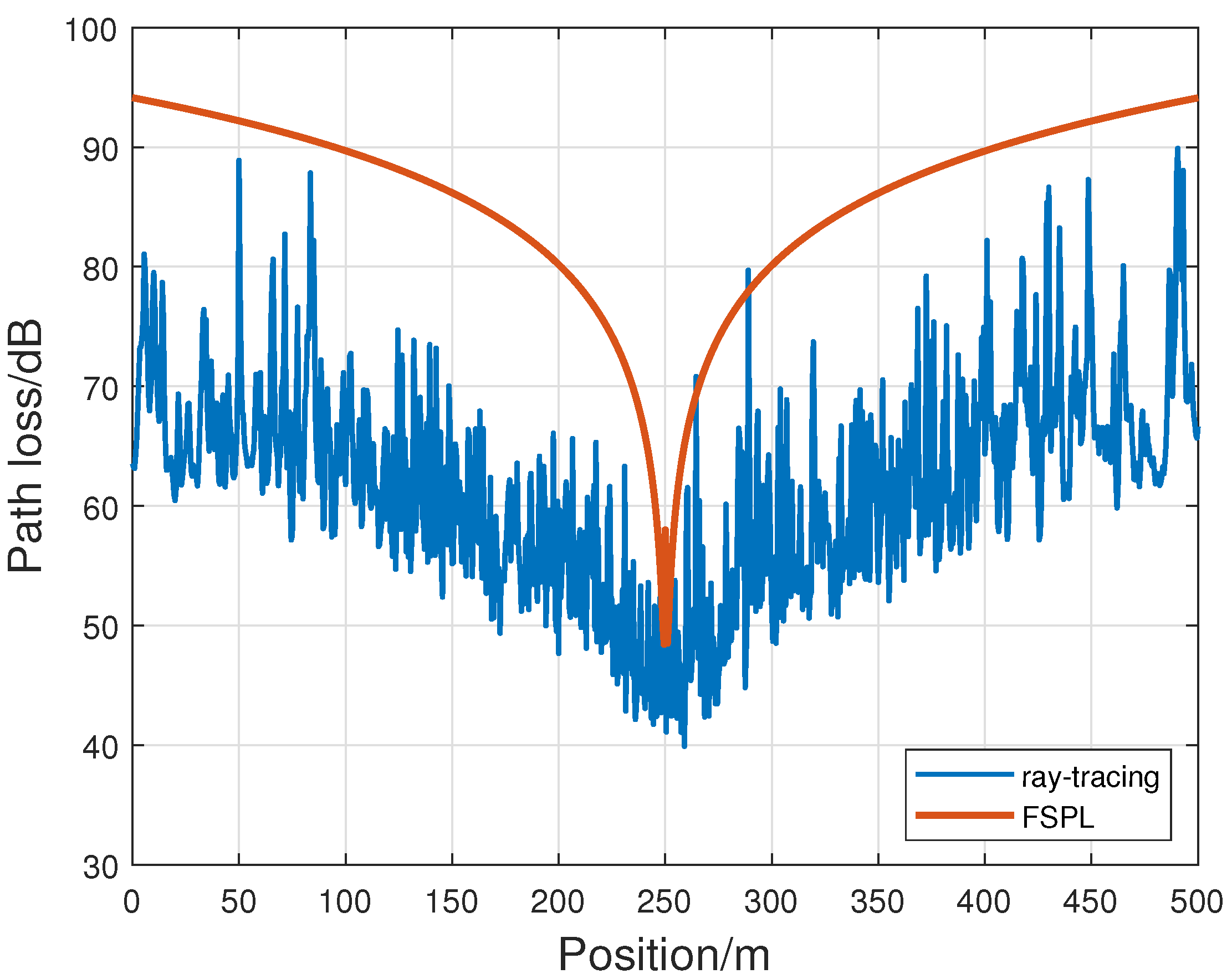
Figure 3 shows the positon-based path loss results. We also plot the free space path loss (FSPL) as a comparison. It can be seen that the path loss in the pipeline decreases first as the train moves closer to the Tx and then increases as the train moves away from the Tx. At the position of 250 m, i.e., the transceiver antenna reaches the same x-axis position, the path loss reaches the lowest value, which conforms to the trend of free space path loss. When the frequency remains constant, the path loss value decreases with the decrease in propagation distance. The path loss shows a high degree of symmetry due to the symmetry of the tube.

Then we focus on establishing the path loss model in the vacuum tube scenario. For the convenience of analysis, we make a data fitting and compare it with other published path loss models. Specifically, the common large-scale fading models include the free space fading model, the free space Closed-in (CI) model, and the Alpha-Beta-Gamma (ABG) model [25].

In the free space fading model, there is no obstacle between the transmitter and receiver, and the propagation medium is ideal and isotropic. According to the Fresnel formula, the path loss in free space can be expressed as

$$P{L}_{\mathrm{free}}=20lg10\left(d\right)+20lg10\left(f\right)-20lg10\left(\frac{c}{4\pi }\right),$$

(12)

where d is the distance between the transceivers in units of kilometers, f is the carrier frequency in units of GHz, and c is the speed of light.

The path loss of the CI model can be expressed as

$$P{L}_{CI}=P{L}_{\mathrm{free}}\left(d_0\right)+10n_{PL}lg\left(\frac{d}{d_0}\right)+X_{SF}^{CI},$$

(13)

where $P{L}_{\mathrm{free}}\left(d_0\right)$ is the free space path loss at the reference distance $d_0$, this value is only related to the frequency but not to the measurement data. It can be calculated as

$$\mathrm{P}{\mathrm{L}}_{free}\left(d_0\right)=20{log}_{10}\left(\frac{4\pi d_0}{\lambda }\right)$$

(14)

$n_{PL}$ is the path loss index. $X_{SF}^{CI}$ is shadow fading, which follows the normal distribution with a mean value of 0.

When the frequency and intercept are fixed, the intercept of the fitting curve of the CI model is fixed. While the measurement scenario, i.e., vacuum tube scenarios, is significantly different from the free space, the CI model is not the best-fitting model based on the measured data, therefore, in this paper, we mainly consider the ABG model. According to the ABG model, the path loss can be expressed as

$$P{L}_{ABG}=A_0+10nlg\left(\frac{d}{d_0}\right)+X_{SF}^{},$$

(15)

where $A_0$ is the path loss at reference distance $d_0$, and it is fitted by the ordinary least squares according to the measurement data. $X_{SF}$ is shadow fading as well. This means that the fitting accuracy of the ABG model is higher than that of the C1 model in the vacuum tube scenarios.

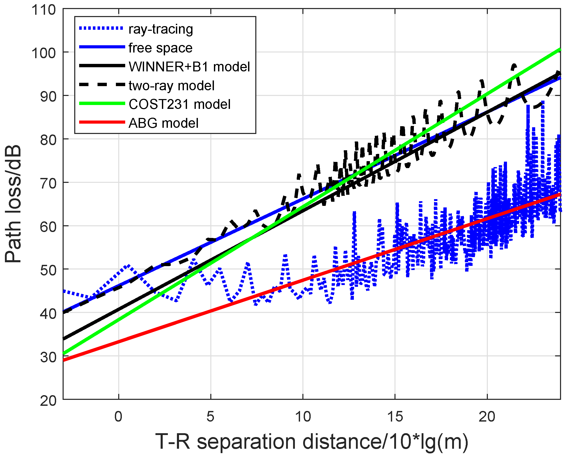
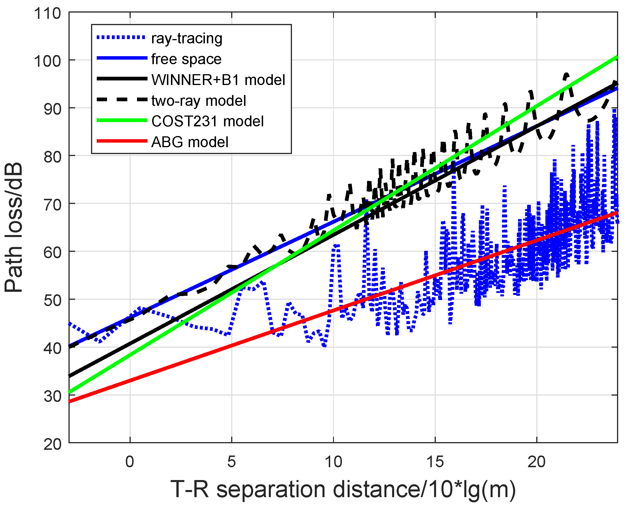
Figure 4 and Figure 5 show the simulation results of path loss at ranges of 0–250 m and 250–500 m, respectively. The x axis in Figure 4 and Figure 5 represents the distance in dB between the Tx and Rx. The y axis in Figure 4 and Figure 5 represents the path loss value. The two figures show the path loss fitting result of the two parts of the tube and we can compare the path loss result of the same distance from the Tx and Rx in the two parts. From the figure, we can know that the path loss values are similar. We use the ABG model to fit these two parts of path loss, respectively. Then we compare results with the free space path loss model, Wireless World Initiative New Radio (WINNER)+B1 model, two-ray model, and COST231 model, respectively. It is obvious that the path loss value in the vacuum tube is lower than that in the free space and open space. This is because the metal surface in the vacuum tube is relatively smooth, resulting in more reflective components. Hence the energy loss of the wireless signal in the transmission process is lower than that in the open space. According to the statistical results, the path loss index of the two parts in the vacuum tube are 1.417 and 1.464, respectively, which are smaller than the path loss index in free space. This characteristic is similar to the path loss results of wireless channels in traditional tunnels.

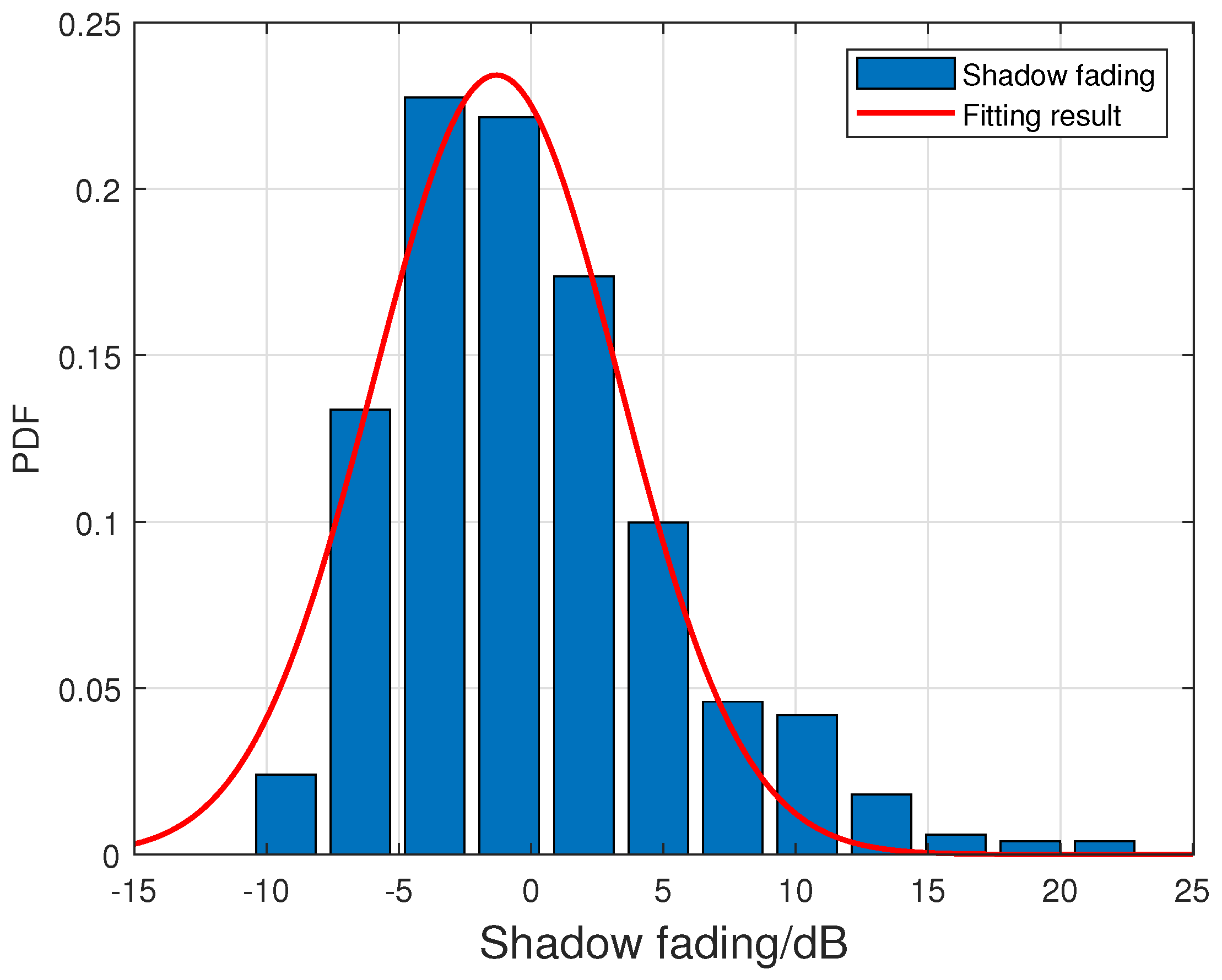
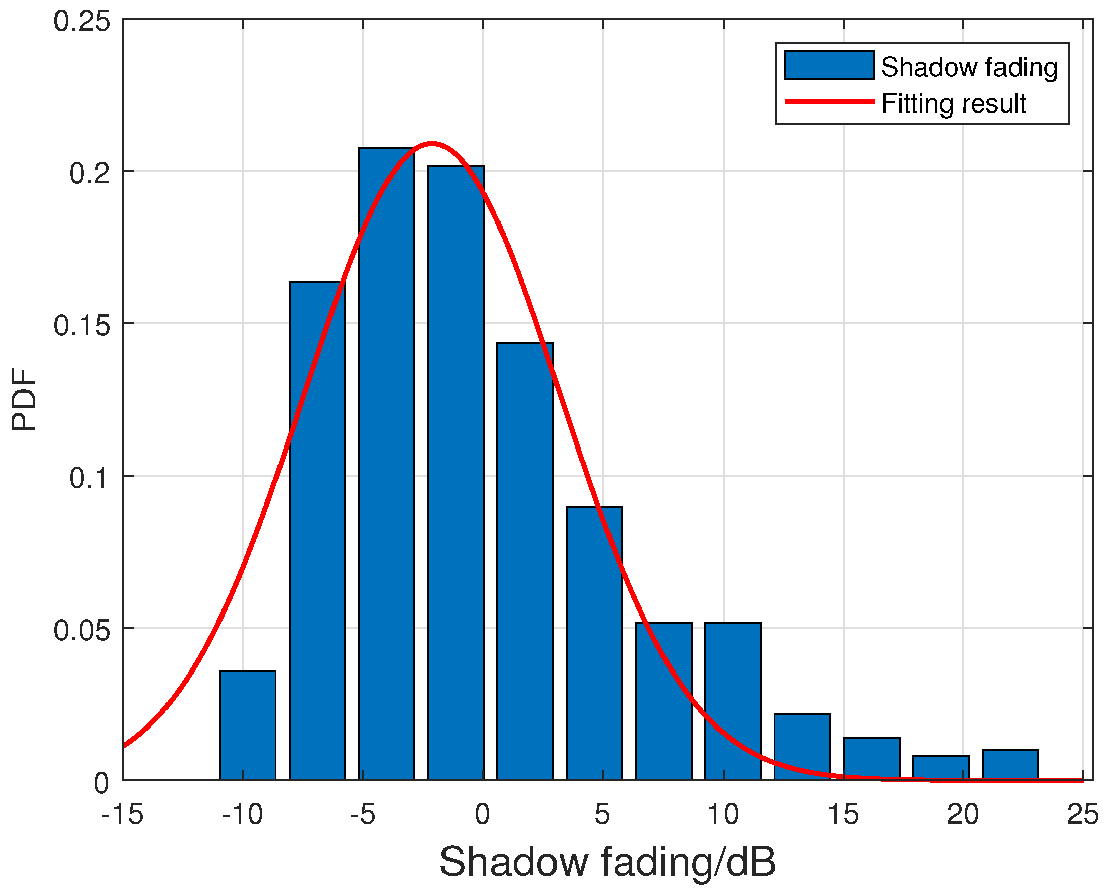
Based on the path loss model fitted by the ABG model, we further made a statistical analysis of shadow fading. Figure 6 and Figure 7 are the statistical analysis results of 0–250 m and 250–500 m, respectively. Then we use the Gaussian distribution to fit it. The probability density functions (PDF) of the fitting results are $\mathcal{N}(-1.32, 6.59)$ and $\mathcal{N}(-2.13, 7.54)$, respectively.

Table 3. Parameters of large-scale fading model.

Position	n	${\mathit{A}}_0$	${\mathit{X}}_{\mathbf{SF}}$
0–250 m	1.42	47.44	5.36
250–500 m	1.46	47.65	6.44

summarizes the parameter values of the large-scale fading model of the ABG model.

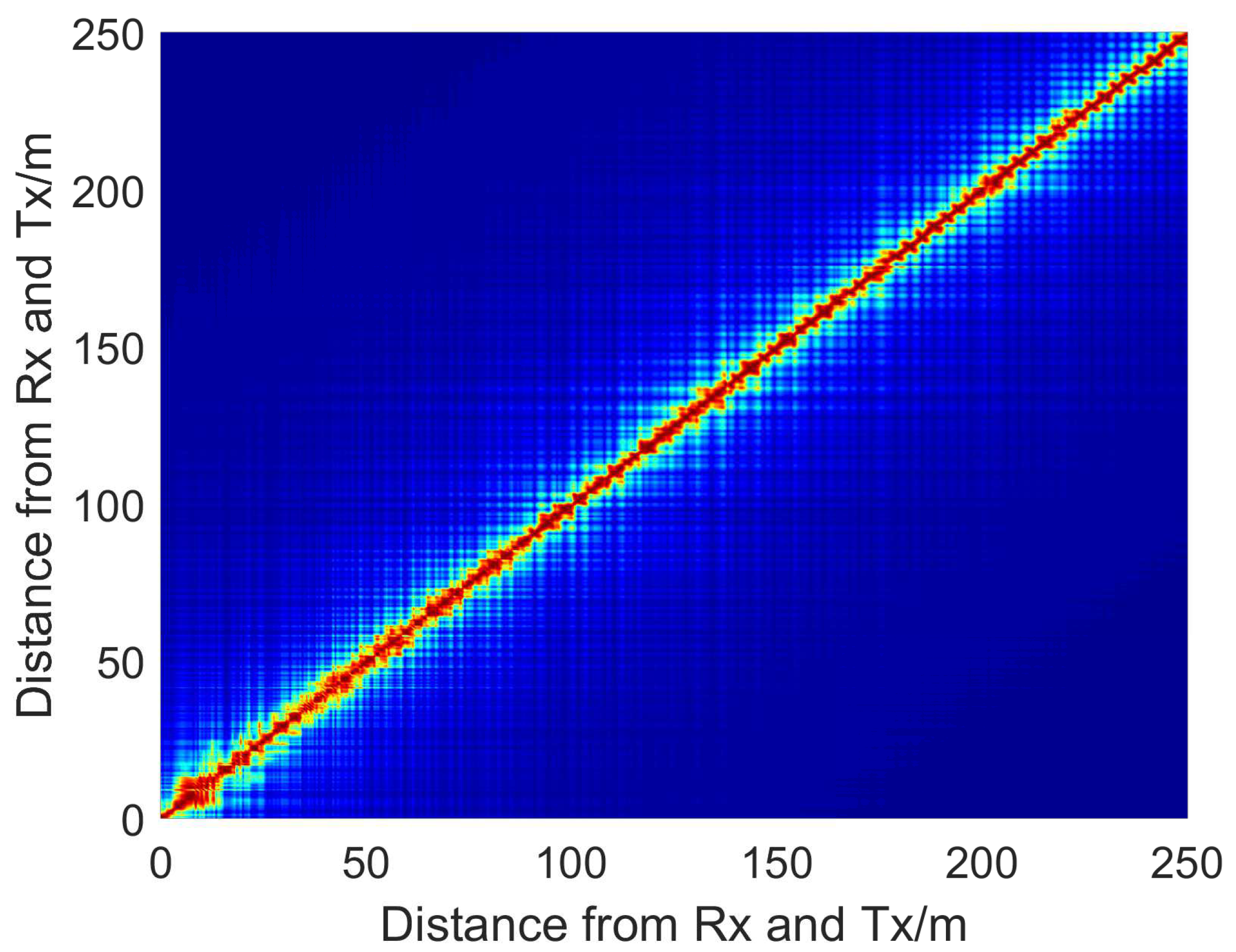
The Pearson correlation coefficient is used to describe the correlation of signals received by antennas at different positions [26], which can be expressed as

$${\rho }_{1,2}=\frac{{\sum }_i\left(∥h_{1,i}∥-\overline{∥h_1∥}\right)\left(∥h_{2,i}∥-\overline{∥h_2∥}\right)}{\sqrt{{{\sum }_i\left(∥h_{1,i}∥-\overline{∥h_1∥}\right)}^2}\sqrt{{{\sum }_i\left(∥h_{2,i}∥-\overline{∥h_2∥}\right)}^2}}$$

(16)

where $h_{1,i}$ and $h_{2,i}$ represent the amplitude of the CIR at ranges of 0–250 m and 250–500 m, respectively. Figure 8 demonstrates that the correlation coefficient of 0–250 m and 250–500 m varies with the movement of the Hyperloop in the vacuum tube scenario. From the figure, we can know that there is a high relevance between the ranges of 0–250 m and 250–500 m when the train is at the same distance from Rx and Tx. The difference is small, and the mean value of the correlation coefficient is 0.95. While the distance from Rx and Tx is different, the correlation coefficient declines rapidly.

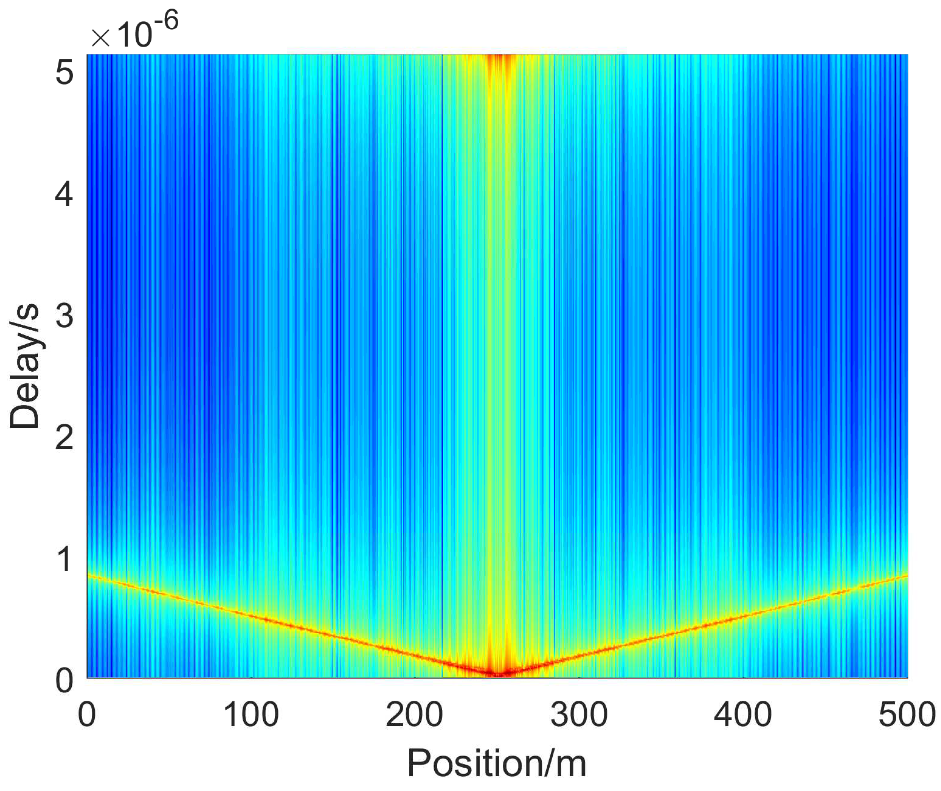
Small-scale fading refers to the fast fluctuation of the signal level of the radio signal in a short distance or a short time. Due to the multipath effect, the mobility of the transmitter and receiver, and the surrounding environment, mobile wireless channels present dispersion in the time domain, frequency domain, and angular domain. According to the results of the Wireless Insite simulation, we collect and summarize 500 m CIR snapshots, as shown in Figure 9. From the figure, we can see the PDP results intuitively. We can observe that the overall CIR delay decreases first and then increases. The transmitting antenna is located on 250 m in the middle, where the CIR has the largest amplitude and the smallest delay. 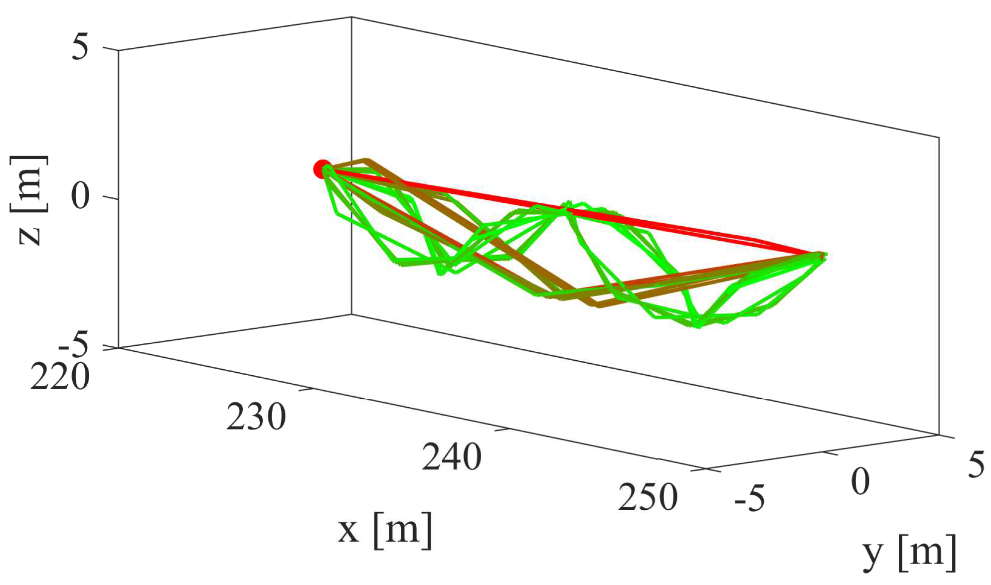Figure 10 is a schematic diagram of multipath. The red line indicates the multipath with high power, and the green line indicates the multipath with low power.

Generally, time delay spread is used to describe the channel dispersion in the time domain quantitatively. Due to the reflection, multipath effects are generated in the radio wave propagation process. Therefore, the received signal is the superposition of multipath signals with different time delays. In the frequency domain, it is shown that the channel has frequency-selective fading characteristics. Root mean square delay spread (RMS-DS) is widely adopted to quantify the time dispersion of the wireless channels [27], which is expressed as

$${\sigma }_{\tau }=\sqrt{\frac{{\displaystyle \sum _{l=1}^L}\left({\tau }_l-\overline{\tau }\right){\left|h\left({\tau }_l\right)\right|}^2}{{\displaystyle \sum _{l=1}^L}{\left|h\left({\tau }_l\right)\right|}^2}},$$

(17)

where L is the total number of all multipath components in a certain time or snapshot, $\overline{\tau }$ is the average delay, which is the first moment of PDP, and it can be calculated as

$$\overline{\tau }=\frac{{\displaystyle \sum _{l=1}^L}{\tau }_l{\left|h\left({\tau }_l\right)\right|}^2}{{\displaystyle \sum _{l=1}^L}{\left|h\left({\tau }_l\right)\right|}^2}$$

(18)

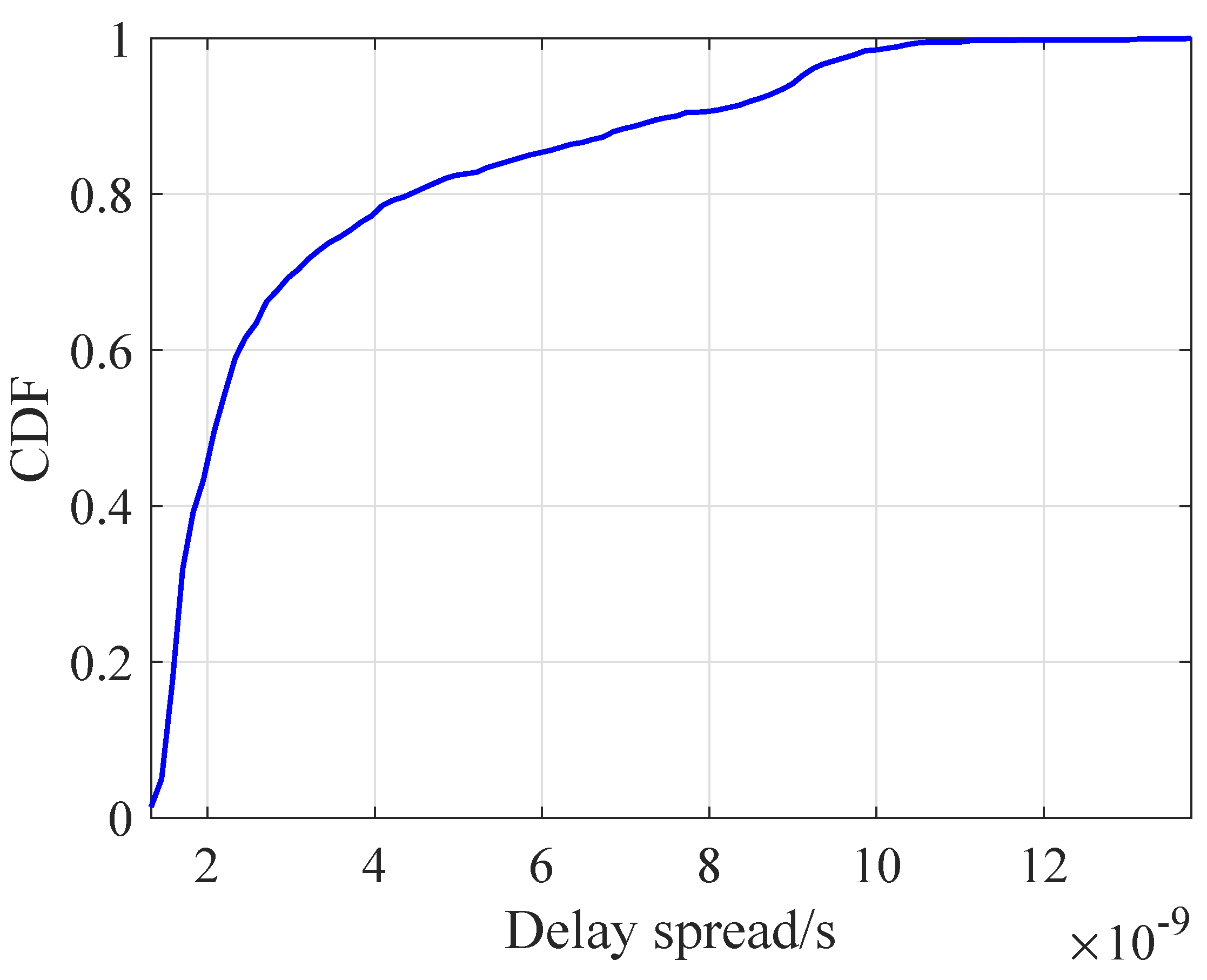
where ${\tau }_l$ and ${\left|h\left({\tau }_l\right)\right|}^2$ are the time delay and power of the l-th tap, respectively. According to the above formula, we can calculate the RMS-DS of each CIR. To better show the delay spread in the vacuum tube scenario, we make the CDF statistics of all snapshots, as shown in Figure 11. The mean of delay spread is 42.13 ns, which is large than the mean of the WINNER B1 model.

Then the angular dispersion is analyzed as well. Multipaths caused by reflection points near the transmitter and receiver in wireless communication lead to different departure angles or arrival angles for multipaths, resulting in dispersion in the angular domain. Angular spread is a key parameter used to describe the spatial selective fading of wireless channels quantitatively. By calculating the second moment of the corresponding angular power distribution, the angular spread gives the measured value of angular dispersion, which is expressed as

$${\sigma }_{\theta }=\sqrt{\frac{{\displaystyle \sum _{l=1}^L}{\theta }_{l,\mu }^2·{\left|h\left({\tau }_l\right)\right|}^2}{{\displaystyle \sum _{l=1}^L}{\left|h\left({\tau }_l\right)\right|}^2}},$$

(19)

where ${\theta }_{l,\mu }$ and $\overline{\theta }$ can be calculated as

$${\theta }_{l,\mu }=mod\left(\left({\theta }_l-\overline{\theta }+\pi ,2\pi \right)\right)-\pi ,$$

(20)

$$\overline{\theta }=\sqrt{\frac{{\displaystyle \sum _{l=1}^L}{\theta }_{l,\mu }·{\left|h\left({\tau }_l\right)\right|}^2}{{\displaystyle \sum _{l=1}^L}{\left|h\left({\tau }_l\right)\right|}^2}},$$

(21)

where $\theta$ represents the angles of AoA or AoD.

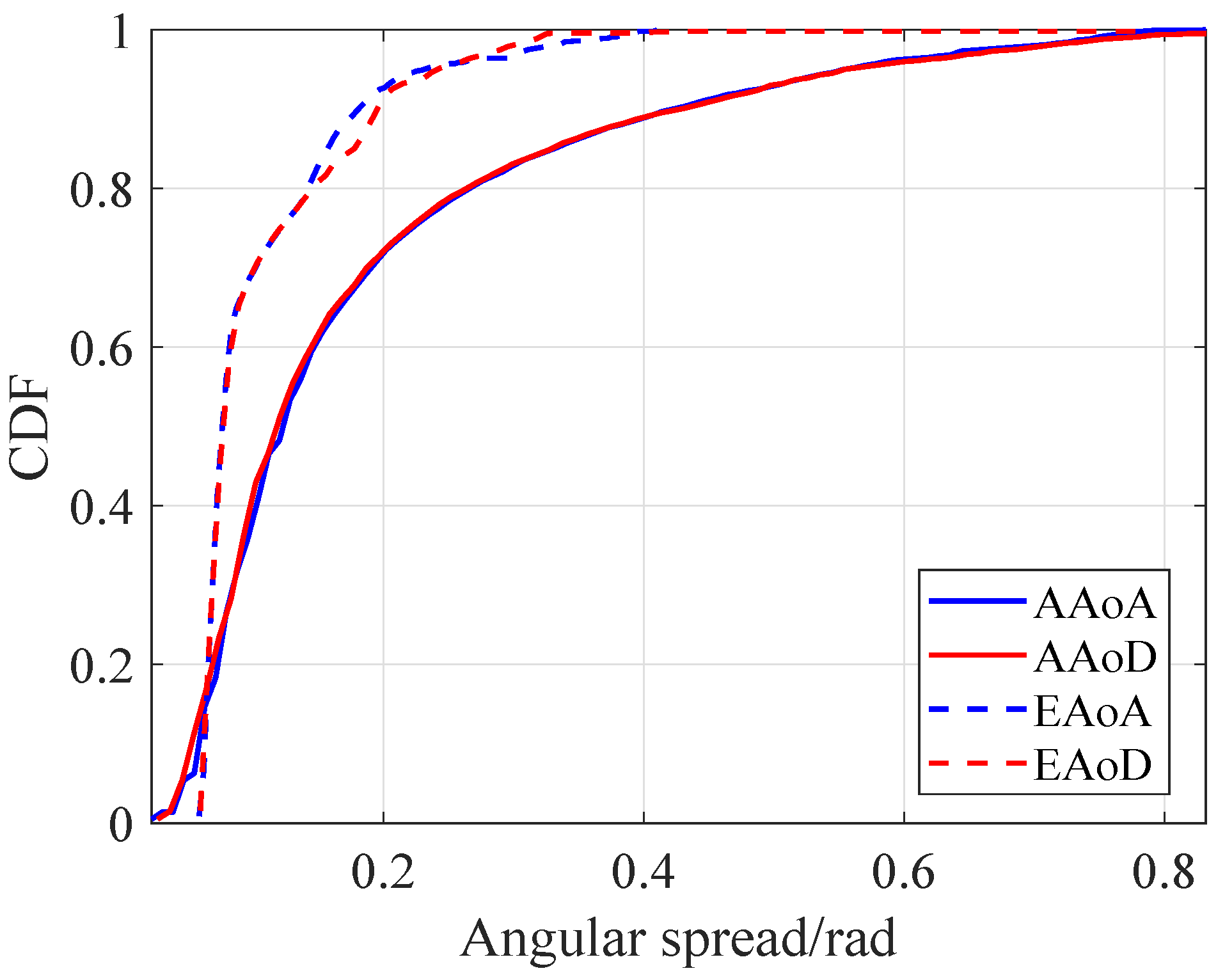
From Figure 12, we can know that the angular spread values of EAoA and EAoD are generally smaller than that of AAoA and AAoD. The AAoA and AAoD angular spread CDF are almost the same, and the angular spread value of EAoA is slightly lower than that of EAoD. The means of the AAoA, AAoD, EAoA, and EAoD angular spread are 0.1871, 0.1864, 0.1060, and 0.1097 rad, respectively.

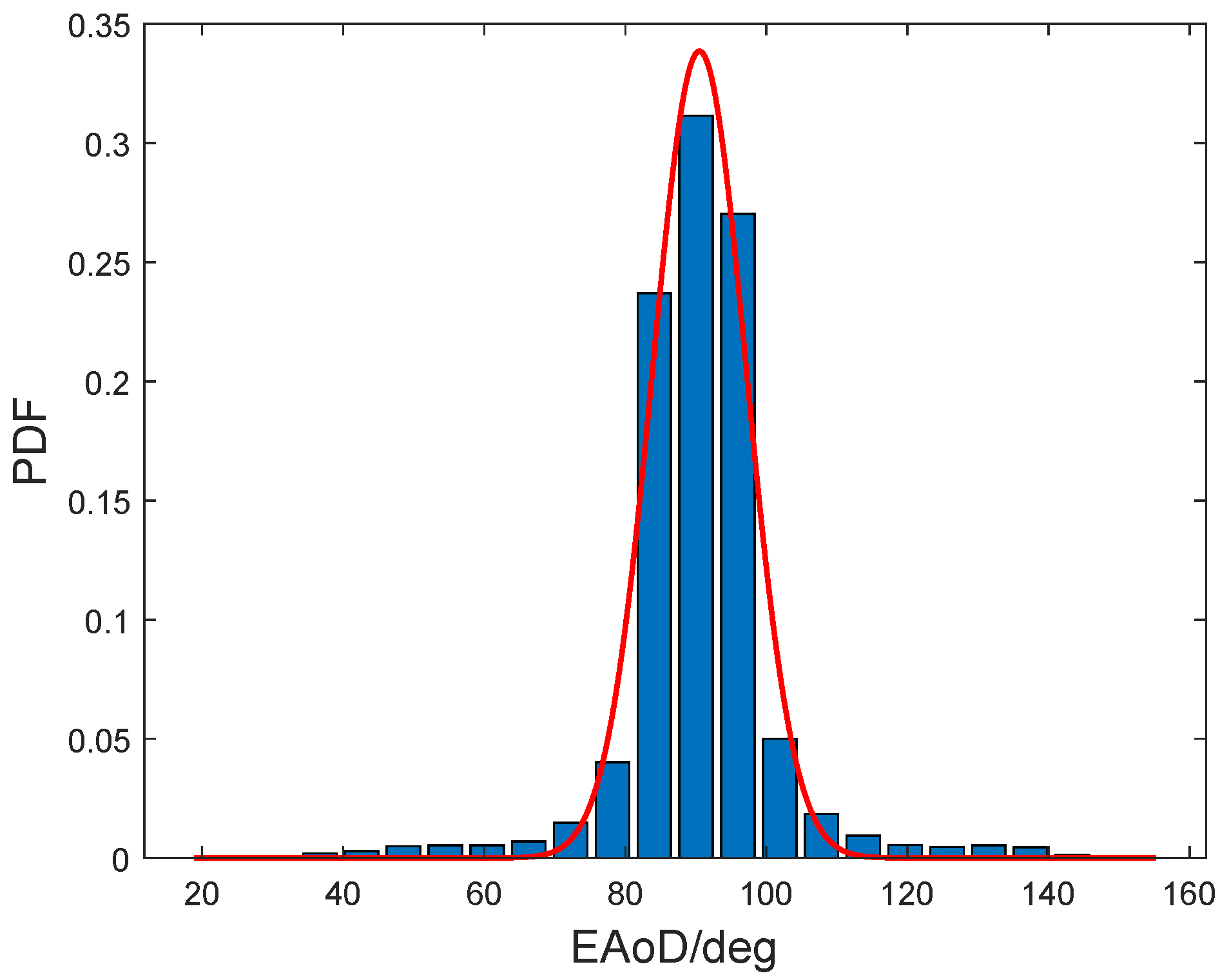
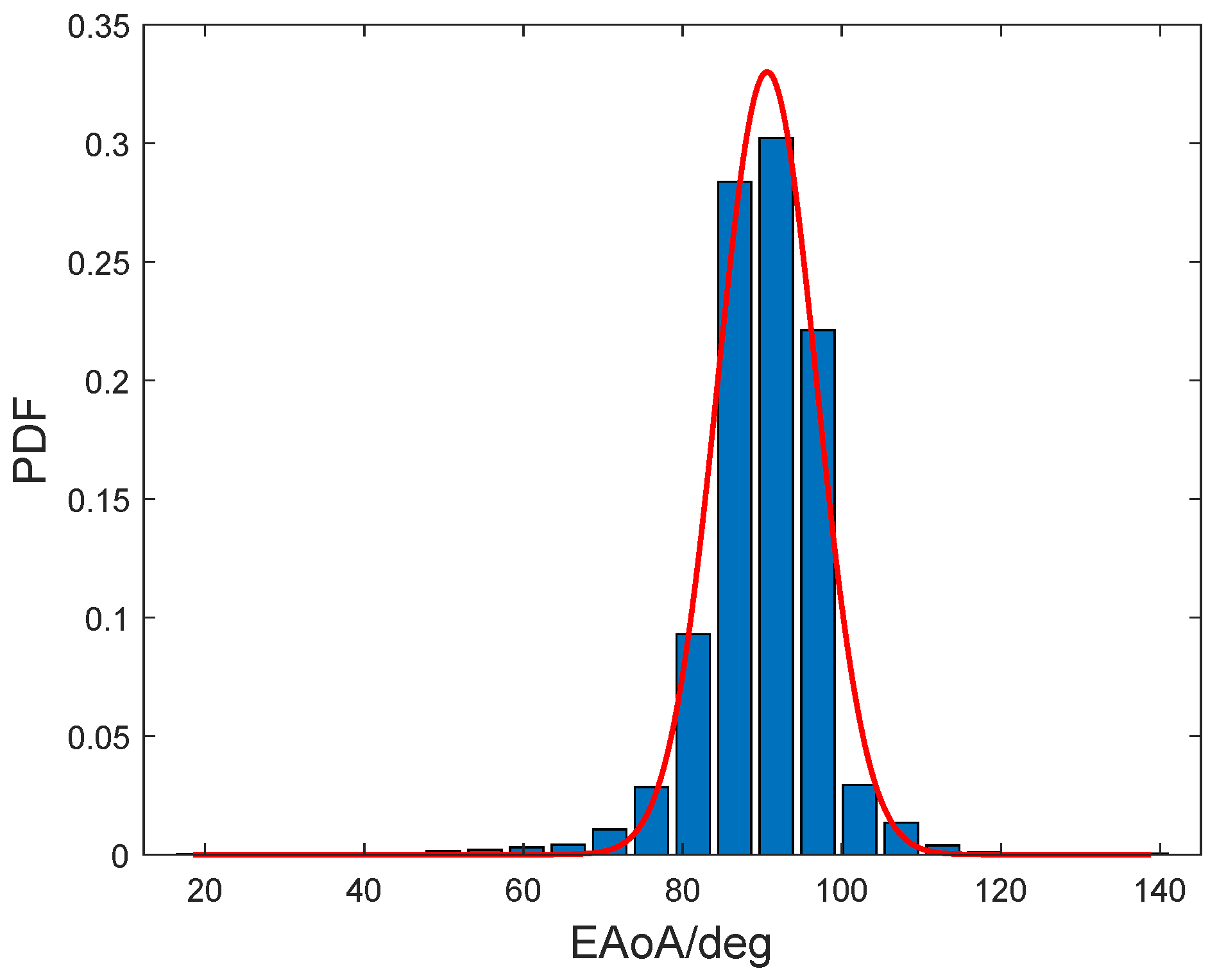
We further make statistics of the angular distribution of 4 kinds of angles. Figure 13 and Figure 14 show the distributions of EAoD and EAoA, respectively. The elevation angles are mainly distributed between 80${}^{\circ }$–100${}^{\circ }$, and we fit it with the Gaussian distribution. The PDF of the fitting results are $\mathcal{N}(90.51, 9.39)$ and $\mathcal{N}(90.62, 8.76)$, respectively. From the figures, we can know that the EAoD and EAoA are mainly around 90 degrees; this is because the transceiver antennas are on the same vertical coordinate axis. 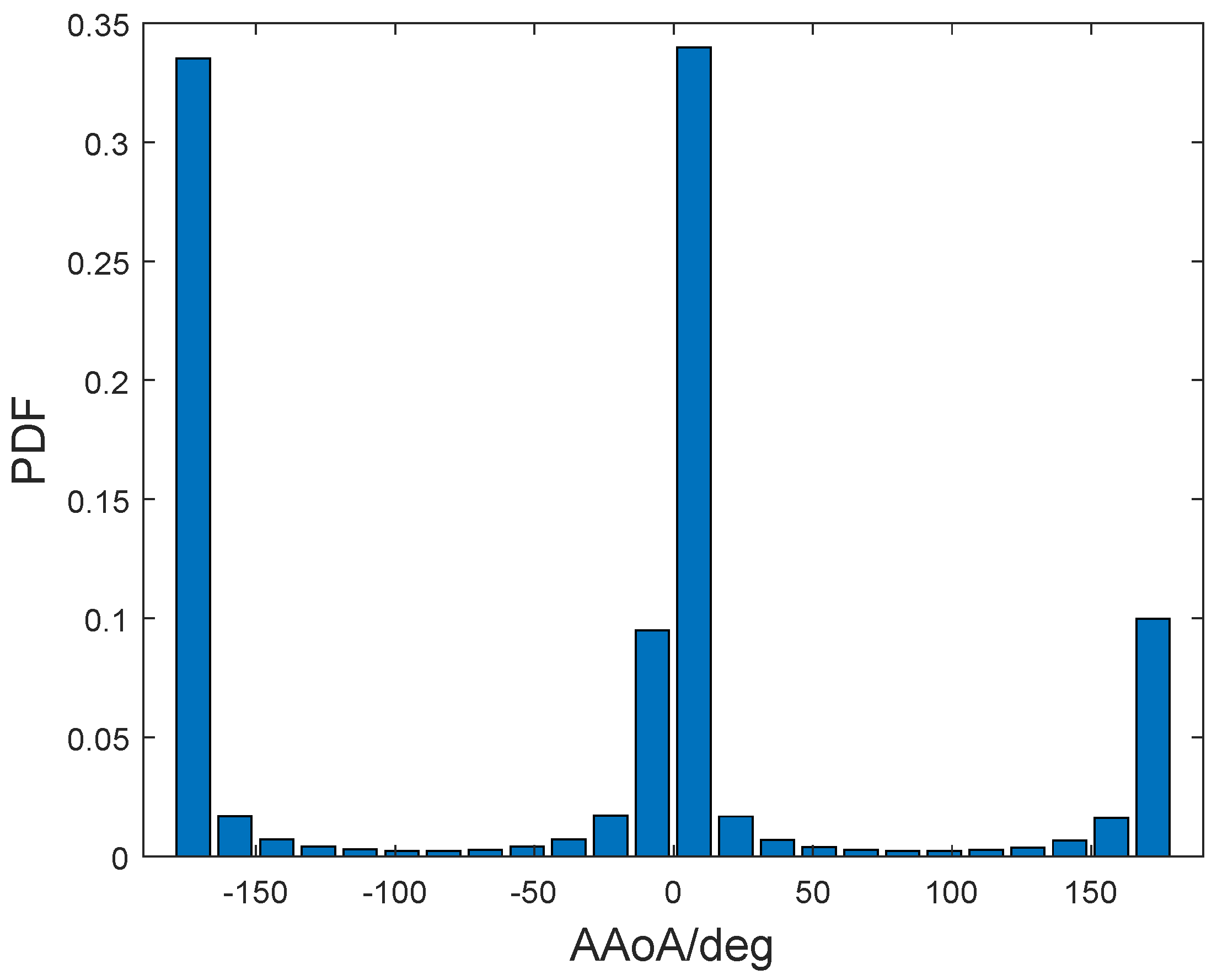Figure 15 and Figure 16 show the distributions of AAoD and AAoA, respectively. For the azimuth angle distribution, it is mainly concentrated around 0, 180, and −180 degrees. The reason is that the Tx and Rx are located on the same line, which determines the azimuth angle of multipath is also along the direction.

5. Conclusions

In this paper, we propose a ray-tracing-based channel model and analyze channel characteristics for Hyperloop scenarios at 4.85 GHz, the 3D environment model of the vacuum tube is constructed. The LoS component and reflection components are considered to derive the CIR expression. All the channel characteristics in the simulation region are extracted in terms of path loss, shadow fading, correlation coefficient, RMS delay spread, angular spread, and the distribution of AOA and AOD. We fit the path loss model in the vacuum tube and compare it with some published models. The path loss index of the two parts in the vacuum tube are 1.417 and 1.464, which are smaller than the path loss index in free space. The shadow fading and the angular distribution are also statistics and fitted by the Gaussian distribution. With this foundation, future work can be done to add the train body of different materials and structures. Consequently, the research of channel characteristics in vacuum tube scenarios is of great significance for the future train-to-ground communication system design of Hyperloop.