
On the P3 Coloring of Graphs


Abstract
1. Introduction
2. Motivation
3. Main Results
- Case I: If , then ;
- Case II: If , then ;
- Case III: If , then .
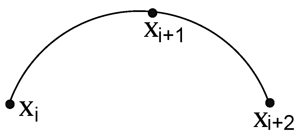
- Case I: Suppose that . Let us define a function f on the vertices of as follows:where . Figure 4 represents the coloring of to explain this labeling. Let be an arbitrary path in , as shown in Figure 5, for .Then, there are three possible cases.
- (a).
- From Figure 5, we have,if , then ;
- (b).
- If , then ;
- (c).
- If , then .
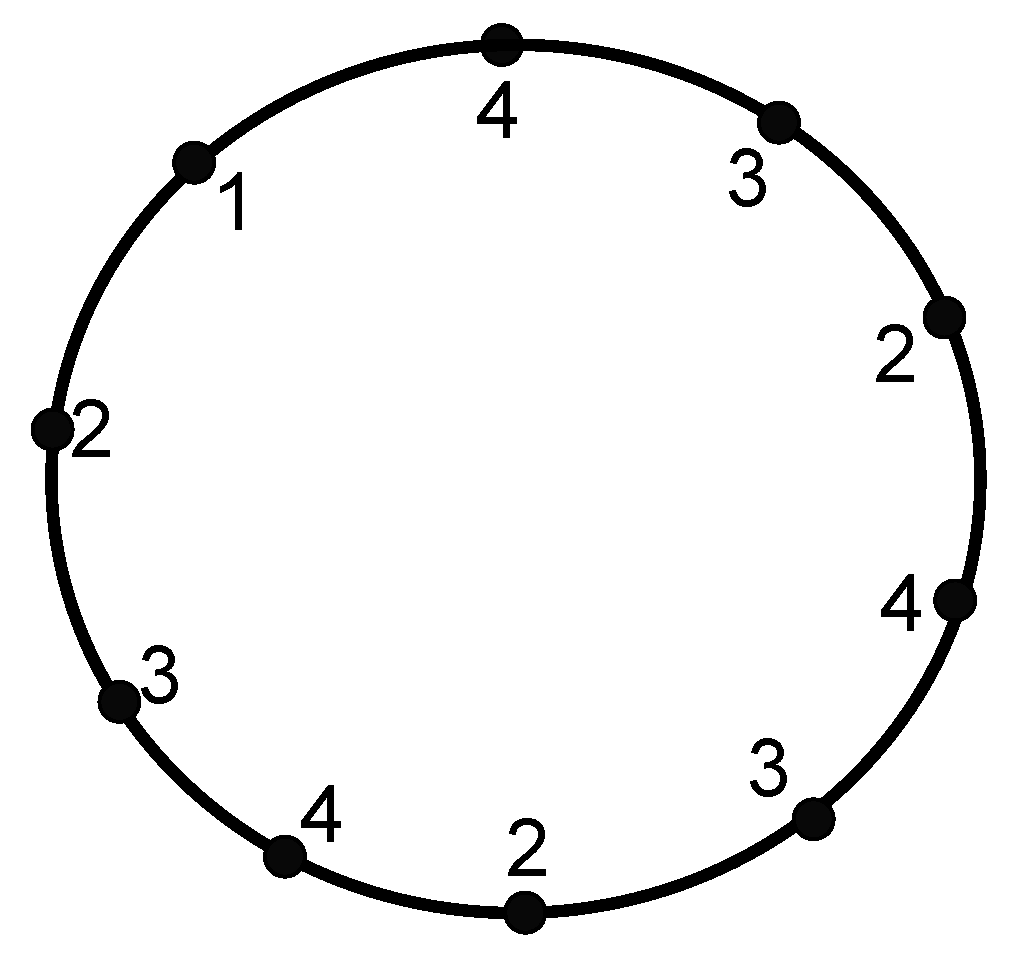
Thus, from all of these cases, we can see that all paths have different colors of their vertices. Thus, f is a coloring, and the result follows. - Case II: Suppose that . In this case, when we start a coloring of from any vertex, e.g., , to the last, e.g., , with at most three colors, then the last vertex cannot be assigned any color from the given three colors. Thus, we need at least four colors to have a coloring of this graph. For the reverse case, we define the -labeling function as follows:and for all we haveFigure 6 represents the coloring of to explain this labeling. Let be an arbitrary path in ; then, there are four possible cases to discuss this labeling.
- (a).
- If , then ;
- (b).
- If , then ;
- (c).
- If , then ;
- (d).
- When the paths are of the forms , , and ;
- (i)
- For the path , we have the labeling ;
- (ii)
- For the path , we have the labeling ;
- (iii)
- For the path , we have the labeling because ;
- (iv)
- For the path , we have the labeling because .Thus, from all of these cases, we can see that all paths have different colors of their vertices. Thus, f is indeed a coloring. This shows that . This concludes the result.
- Case III: When . In this case, to start a coloring of from vertex to the last with at most three colors, the last two vertices , cannot be assigned any color from the given three colors. Therefore, we need at least four colors to have coloring of this graph. For the reverse case, we will define labeling function as follows:, , , , and for all , the function is defined byTo explain this labeling, Figure 7 shows a coloring of under f. Let be any arbitrary path in ; then, we have the following cases to discuss for the assertion of coloring.
- (a).
- If and , then ;
- (b).
- If and , then ;
- (c).
- If and , then ;
- (d).
- For the following paths, we have different labeling:
- (i)
- For path , we have the labeling ;
- (ii)
- For path , we have the labeling ;
- (iii)
- For path , we have the labeling , because ;
- (iv)
- For path , we have the labeling , because .Therefore, from all of these cases, we can see that all paths have different colors of their vertices. Thus, f is a coloring and for all . Hence, the proof is completed.
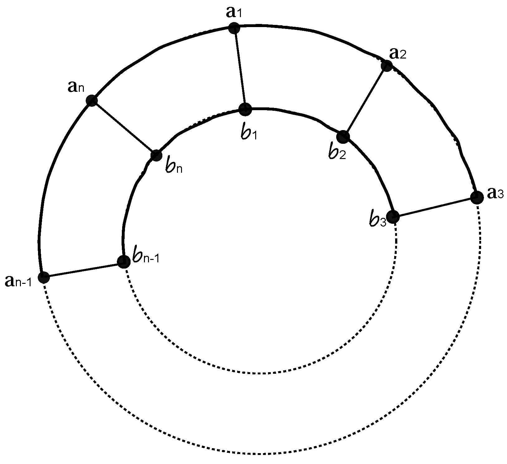
- Case I. Assume that and . Since is a subgraph of , then from Theorem 1, we have . To prove the reverse, we shall define a function as follows:We will show that f is a coloring. Let be any arbitrary path in ; then, there are ten possible types of paths in , and they are as follows: The paths are , , , , , , , , and .
- (a).
- For , we have ten possibilities of the induced coloring of from g as follows:
- (i)
- If the path is , then we have ;
- (ii)
- If the path is , then we have ;
- (iii)
- If the path is , then we have ;
- (iv)
- If the path is , then we have ;
- (v)
- If the path is , then we have ;
- (vi)
- If the path is , then we have ;
- (vii)
- If the path is , then we have ;
- (viii)
- If the path is , then we have ;
- (ix)
- If the path is , then we have ;
- (x)
- If the path is , then we have .
- (b).
- For , we have ten possibilities of the induced coloring of from g as follows:
- (i)
- If the path is , then we have ;
- (ii)
- If the path is , then we have ;
- (iii)
- If the path is , then we have ;
- (iv)
- If the path is , then we have ;
- (v)
- If the path is , then we have ;
- (vi)
- If the path is , then we have ;
- (vii)
- If the path is , then we have , ;
- (viii)
- If the path is , then we have , ;
- (ix)
- If the path is , then we have , ;
- (x)
- If the path is , then we have , .
- (c).
- For , we again have ten possibilities of the induced coloring of from g as follows:
- (i)
- If the path is , then we have ;
- (ii)
- If the path is , then we have ;
- (iii)
- If the path is , then we have ;
- (iv)
- If the path is , then we have ;
- (v)
- If the path is , then we have ;
- (vi)
- If the path is , then we have ;
- (vii)
- If the path is , then we have , ;
- (viii)
- If the path is , then we have , ;
- (ix)
- If the path is , then we have , ;
- (x)
- If the path is , then we have , .
- (d).
- For , we have ten possibilities of the induced coloring of from g as follows:
- (i)
- If the path is , then we have ;
- (ii)
- If the path is , then we have ;
- (iii)
- If the path is , then we have ;
- (iv)
- If the path is , then we have ;
- (v)
- If the path is , then we have ;
- (vi)
- If the path is , then we have ;
- (vii)
- If the path is , then we have , ;
- (viii)
- If the path is , then we have , ;
- (ix)
- If the path is , then we have , ;
- (x)
- If the path is , then we have , .
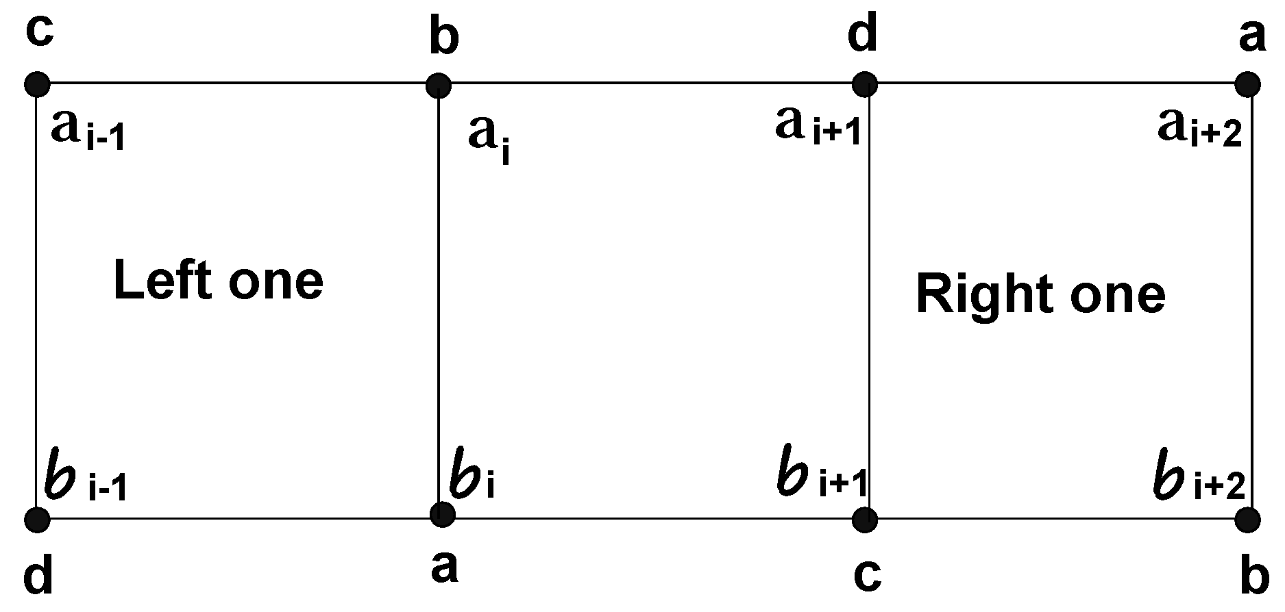
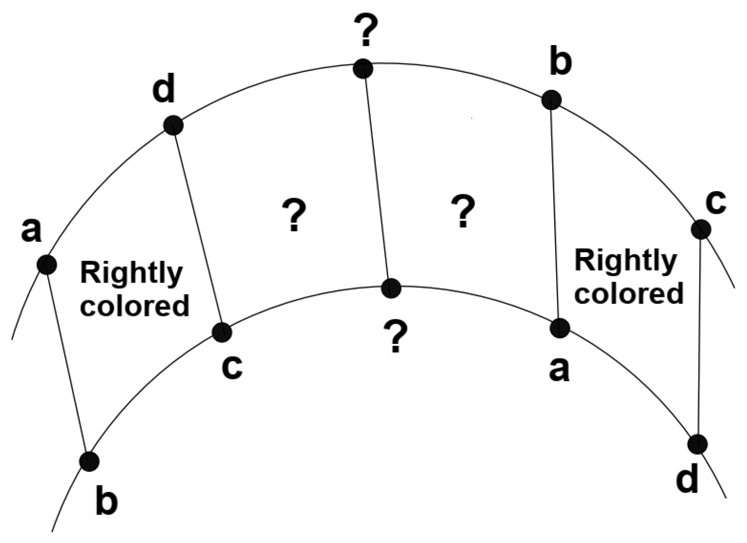
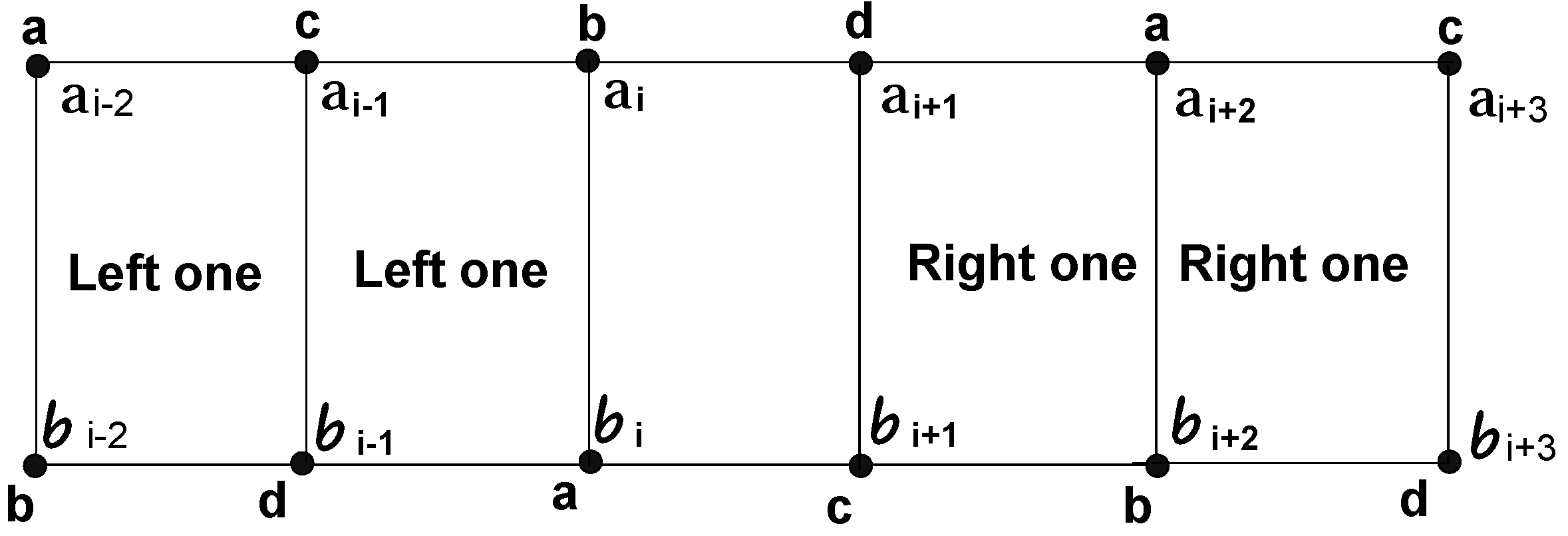
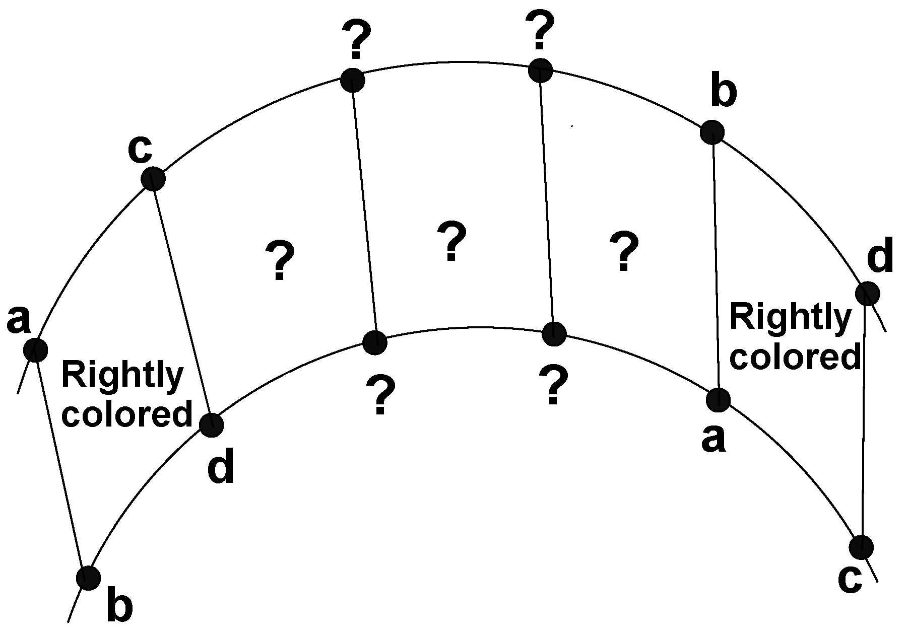
In all of these subcases, we can see that g is indeed a coloring. Therefore, the -chromatic number of prism graph is 4 for all and . - Case II. Assume that and . Note that in any coloring, if we color the vertices of the graph from a set of only four colors , because graph is a subgraph of , then all of the vertices of every have different colors, as shown in Figure 9.Therefore, when we apply any coloring on , for any subgraph, its left and right adjacent ’s have the only possible coloring, as shown in Figure 10.Now, this process is continued until a -coloring with only four colors is completed or produced. We define a to be correctly colored if all its vertices have different colors. Because , and we have n number of s that covers , eventually, we will arrive at a situation displayed in Figure 11.Since , from Figure 11, we can easily see that the remaining two s cannot be correctly colored with only four given colors. Thus, we have , and this shows that we need at least five colors to produce a coloring of . For the reverse case, let us define a function g from to as follows:, ,Let be an arbitrary path; then, as before, there will be ten possible paths for any given . It is enough to discuss the following possible paths to prove that g is indeed a coloring: , , , , , , , , and the last one is , for all .It is clear from the above definition that the remaining paths satisfy the coloring, as depicted in Figure 12.Now, we will show that g is indeed coloring in four cases, which are discussed below.
- (a).
- For and , all possibilities of are discussed as follows:
- (i)
- If the path is , then we have ;
- (ii)
- If the path is , then we have ;
- (iii)
- If the path is , then we have ;
- (iv)
- If the path is , then we have ;
- (v)
- If the path is , then we have ;
- (vi)
- If the path is , then we have ;
- (vii)
- If the path is , then we have , ;
- (viii)
- If the path is , then we have , ;
- (ix)
- If the path is , then we have , ;
- (x)
- If the path is , then we have , .
- (b).
- For , all possibilities of are discussed as follows:
- (i)
- If the path is , then we have ;
- (ii)
- If the path is , then we have ;
- (iii)
- If the path is , then we have ;
- (iv)
- If the path is , then we have ;
- (v)
- If the path is , then we have ;
- (vi)
- If the path is , then we have ;
- (vii)
- If the path is , then we have , ;
- (viii)
- If the path is , then we have , ;
- (ix)
- If the path is , then we have , ;
- (x)
- If the path is , then we have , .
- (c).
- For , all possibilities of are discussed as follows:
- (i)
- If the path is , then we have ;
- (ii)
- If the path is , then we have ;
- (iii)
- If the path is , then we have ;
- (iv)
- If the path is , then we have ;
- (v)
- If the path is , then we have ;
- (vi)
- If the path is , then we have ;
- (vii)
- If the path is , then we have , ;
- (viii)
- If the path is , then we have , ;
- (ix)
- If the path is , then we have , ;
- (x)
- If the path is , then we have , .
- (d).
- For , all possibilities of are discussed as follows:
- (i)
- If the path is , then we have ;
- (ii)
- If the path is , then we have ;
- (iii)
- If the path is , then we have ;
- (iv)
- If the path is , then we have ;
- (v)
- If the path is , then we have ;
- (vi)
- If the path is , then we have ;
- (vii)
- If the path is , then we have , ;
- (viii)
- If the path is , then we have , ;
- (ix)
- If the path is , then we have , ;
- (x)
- If the path is , then we have , .
Thus, in this case, all of these subcases proved that g is a coloring of for . Therefore, . - Case III. Assume that and . Similarly, as in case II, when we apply any coloring on with only four given colors , for any subgraph in , its left and right adjacent ’s have the only possible coloring labels, as shown in Figure 13.We continue this process to complete (or produce) a coloring with only four colors and d. Because , and we have n number of subgraphs that covers , eventually, we will reach the situation displayed in Figure 14.Thus, in the case when , from Figure 14, we can easily see that the remaining three s cannot be correctly colored with only four given colors. Thus, we have . Therefore, we need at least five colors to produce a coloring of . For the reverse case, let us define a function g from to as follows:, .Let be an arbitrary path; then, similarly as in case I and case II, it is very easy to see that g is indeed a coloring. Together with the argument at the beginning of this case, this proves that the -chromatic number of a prism graph is equal to 5 for for all .
- Case IV. Assume that and . Similarly to case II, whenever we apply any coloring on with only four colors , for any subgraph in , its left and right adjacent ’s have the only possible -coloring labels, as shown in Figure 10.
4. Open Problems and Time Complexity
- Problem 1: Prove or disprove the conjecture that “The coloring is an NP-hard problem”;
- Problem 2: Discuss all types of time complexity of coloring as an NP-hard problem;
- Problem 3: Find stronger upper and lower bounds of the coloring;
- Problem 4: Find for .
5. Conclusions
Author Contributions
Funding
Data Availability Statement
Acknowledgments
Conflicts of Interest
References
- Coxeter, H.S.M. The Mathematics of Map Coloring. Leonardo 1971, 4, 273–277. [Google Scholar] [CrossRef]
- Formanowicz, P.; Tanaś, K. A survey of Graph coloring-Its types, methods and applications. Found. Comput. Decis. Sci. 2012, 37, 223–238. [Google Scholar] [CrossRef]
- Burke, E.K.; Meisels, A.; Petrovic, S.; Qu, R. A graph-based hyper heuristic for timetabling problems. Eur. J. Oper. Res. 2007, 176, 177–192. [Google Scholar] [CrossRef]
- Galinier, P.; Hertz, A. A survey of local search methods for graph coloring. Comput. Oper. Res. 2006, 33, 2547–2562. [Google Scholar] [CrossRef]
- Leighton, F. A graph coloring algorithm for large scheduling problem. J. Res. Natl. Burean Stand. 1979, 84, 489–503. [Google Scholar] [CrossRef]
- Philippe, G.; Jean, P.; Hao, K.J.; Daniel, P. Recent Advances in Graph Vertex Coloring; Intelligent Sysstem References Liberary; Springer: Berlin/Heidelberg, Germany, 2013. [Google Scholar]
- Błażewicz, J.; Ecker, K.H.; Pesch, E.; Schmidt, G.; Weglarz, J. Scheduling Computer and Manufacturing Process; Springer: Berlin/Heidelberg, Germany, 1996. [Google Scholar]
- Dewerra, D. An introduction to timetabling. Eur. J. Operrational Res. 1985, 19, 151–162. [Google Scholar] [CrossRef]
- Chow, F.C.; Hennessy, J.L. The priorty-based coloring approach to register allocation. ACM Trans. Program. Lang. Syst. 1990, 12, 501–536. [Google Scholar] [CrossRef]
- Chaitin, G.J.; Auslander, M.A.; Chandra, A.K.; Cocke, J.; Hopkins, M.E.; Markstein, P.W. Register allocation via coloring. Comput. Lang. 1981, 6, 47–57. [Google Scholar] [CrossRef]
- Donderia, V.; Jana, P.K. A novel scheme for graph coloring. Procedia Technol. 2012, 4, 261–266. [Google Scholar] [CrossRef]
- Garey, M.; Johnson, D.; So, H. An Application of graph coloring to printed cicuit testing. IEEE Trans. Circuits Syst. 1976, 23, 591–599. [Google Scholar] [CrossRef]
- Glass, C. Bag rationalization for a food manufacturer. J. Oper. Res. Soc. 2002, 53, 544–551. [Google Scholar] [CrossRef]
- Arputhamarya, A.; Mercy, M.H. Rainbow Coloring of shadow Graphs. Int. J. Pure Appl. Math. 2015, 6, 873–881. [Google Scholar]
- Zufferey, N.; Amstutz, P.; Giaccari, P. Graph coloring approaches for a satellite range sceduling problems. J. Sceduling 2008, 11, 263–277. [Google Scholar] [CrossRef]
- Gamst, A. Some lower bounds for a class of frequency assignment problems. IEEE Trans. Veh. Echonol. 1986, 35, 8–14. [Google Scholar] [CrossRef]
- Voloshin, V.I. Graph Coloring: History, results and open problems. Ala. J. Math. 2009. Available online: https://ajmonline.org/2009/voloshin.pdf (accessed on 2 February 2023).
- Dey, A.; Son, L.H.; Kumar, P.K.K.; Selvachandran, G.; Quek, S.G. New Concepts on Vertex and Edge Coloring of Simple Vague Graphs. Symmetry 2018, 10, 373. [Google Scholar] [CrossRef]
- Gallian, G.A. A Dynamic Survey of Graph Labeling. Electron. J. Comb. 2022, 1, DS6. [Google Scholar] [CrossRef]
- Szabo, S.; Zavalnij, B. Graph Coloring via Clique Search with Symmetry Breaking. Symmetry 2022, 14, 1574. [Google Scholar] [CrossRef]
- Yegnanarayanan, V.; Yegnanarayanan, G.N.; Balas, M. On Coloring Catalan Number Distance Graphs and Interference Graphs. Symmetry 2018, 10, 468. [Google Scholar] [CrossRef]
- Ascoli, A.; Weiher, M.; Herzig, M.; Slesazeck, S.; Mikolajick, T.; Tetzlaff, R. Graph Coloring via Locally-Active Memristor Oscillatory Networks. J. Low Power Electron. Appl. 2022, 12, 22. [Google Scholar] [CrossRef]
- Sotskov, Y.N. Mixed Graph Colorings: A Historical Review. Mathematics 2020, 8, 385. [Google Scholar] [CrossRef]
- Tilley, J.A. The a-graph coloring problem. Discret. Appl. Math. 2017, 217, 304–317. [Google Scholar] [CrossRef]


Disclaimer/Publisher’s Note: The statements, opinions and data contained in all publications are solely those of the individual author(s) and contributor(s) and not of MDPI and/or the editor(s). MDPI and/or the editor(s) disclaim responsibility for any injury to people or property resulting from any ideas, methods, instructions or products referred to in the content. |
© 2023 by the authors. Licensee MDPI, Basel, Switzerland. This article is an open access article distributed under the terms and conditions of the Creative Commons Attribution (CC BY) license (https://creativecommons.org/licenses/by/4.0/).
Share and Cite
Yang, H.; Naeem, M.; Qaisar, S. On the P3 Coloring of Graphs. Symmetry 2023, 15, 521. https://doi.org/10.3390/sym15020521
Yang H, Naeem M, Qaisar S. On the P3 Coloring of Graphs. Symmetry. 2023; 15(2):521. https://doi.org/10.3390/sym15020521
Chicago/Turabian StyleYang, Hong, Muhammad Naeem, and Shahid Qaisar. 2023. "On the P3 Coloring of Graphs" Symmetry 15, no. 2: 521. https://doi.org/10.3390/sym15020521
APA StyleYang, H., Naeem, M., & Qaisar, S. (2023). On the P3 Coloring of Graphs. Symmetry, 15(2), 521. https://doi.org/10.3390/sym15020521