First-Principles Calculation of Ligand Field Parameters for L-Edge Spectra of Transition Metal Sites of Arbitrary Symmetry

Abstract

Recently we have proposed a simple method for obtaining the parameters of a ligand field multiplet model for L-edge spectra calculations from density functional theory. Here we generalize the method to systems where the metal site has arbitrary point symmetry. The ligand field-induced splitting of the metal d-level becomes a hermitian matrix with cross-terms between the different d-orbitals. The anisotropy of the covalency is fully taken into account and it rescales the electron–electron interaction and the oscillator strength in an orbital-dependent way. We apply the method to polarization-dependent V L-edge spectra of vanadium pentoxide and obtain very good agreement with the experiment.

1. Introduction

Ligand field multiplet theory (LFMT) is the standard method for analyzing optical and X-ray spectra involving transition to 3d and 4f valence shells in transition metal and rare-earth compounds [1]. It is an invaluable tool for coordination chemistry, photo-chemistry and X-ray absorption spectroscopy [2,3]. LFMT is based on a single ion model, where intra-atomic electron–electron interactions are accurately described by using a multi-configurational wave function. The perturbation by the rest system is reduced to a local potential, the ligand field (LF) acting on the metal atom. The LF splits the $2l+1$-fold orbitally degenerate free atom shell with angular momentum l, into several sub-levels, according to the point symmetry at the metal center. The LF splitting can be described by a few independent parameters. In the case of a transition metal ion in cubic symmetry, for example, the $3d$-level splits into three-fold ($t_{2g}$) and two-fold ($e_g$) sub-levels, whose energy difference corresponds to the LF parameter $10Dq$. Despite its simplicity, LFMT has been very successful in reproducing experimental spectra, and provides important insight into the electronic and magnetic state of the metal center. The major drawback of the method is that it relies on empirical parameters, namely the LF energy splittings and a reduction parameter of the Coulomb integrals, which accounts for partial delocalization of the atomic orbitals by ligand bonding (also known as the nephelauxetic effect [4]). Various schemes have been presented for extracting LF parameters from ab initio calculations [5,6,7]. Most of these methods focus on the weak ligand field of rare-earth $4f$ shells and/or are tied to specific quantum chemistry codes, e.g., ADF [8]. As a result, they have not found wide-spread use in the community of X-ray spectroscopists, who still largely rely on adjusting the LF parameters to the experimental spectra. Since the number of LF parameters increases with decreasing symmetry, the need for non-empirical parameter determination is particularly strong for low symmetry systems. Indeed, while in octahedral symmetry, there is only one LF parameter ($10Dq$), the number of independent parameters rises to 14 for the lowest possible symmetry ($C_1$ group). Additionally, Coulomb integral reduction factors are needed to describe the nephelauxetic effect. If the anisotropy of the covalency is to be taken account of, the number of independent reduction parameters can be as large as 15 (for $C_1$ symmetry), which would give a total of 29 independent parameters. It is clear that fitting such a large number of empirical parameters to a single experimental X-ray absorption spectrum is both mathematically ill-defined and physically meaningless. Metal ions at low symmetry sites are very common in catalytic active systems and biological molecules. When empirical LFMT is applied to such systems, an approximate, higher point symmetry is often assumed [9] without theoretical justification and with uncertain outcome.

In Ref. [10] we have presented a simple, non-empirical scheme for obtaining the LF parameters ab initio from the output of standard density functional theory (DFT) codes. The anisotropy of the nephelauxetic effect has also been taken into account. These features were implemented in a home-written LFMT code [11]. The method was tested on transition metal monoxide crystals and metal phthalocyanine molecules and good results were obtained in all cases [10]. In those examples, the point symmetry was high ($O_h$ or $D_{4h}$), such that the five d-orbitals are not mixed by the LF, i.e., the LF matrix is diagonal. This fact justified a number of simplifying theoretical assumptions that were made in [10], but which do not hold in the case of arbitrarily low symmetry.

Here we generalize the method of Ref. [10] to arbitrary symmetry and successfully apply it to the V L-edge spectra of V${}_2$O${}_5$ where the metal site has very low symmetry ($C_s$).

2. Theory

We consider a single metal atom center in a molecular or solid system, whose valence orbitals are ${\psi }_k\left(\mathbf{r}\right)=\langle \mathbf{r}|k\rangle$ with energy $E_k$. Throughout this paper we assume a non-magnetic ground state and suppress the spin quantum number. The theory can easily be extended to allow for a possible spin-dependence of the LF in magnetic systems. In the LFMT we focus on the valence l-shell ($l=2$ or 3) of the atom with its $2l+1$ orbitals $|m\rangle$, $m=1,\dots 2l+1$. The molecular orbitals $|k\rangle$ are projected on the l-shell atomic orbitals:

$$|k\rangle =\sum _m|m\rangle \langle m|k\rangle +|\tilde{k}\rangle$$

(1)

where $|\tilde{k}\rangle$ is the ligand part of the molecular orbital, or more precisely, all of the rest of the molecular orbital without the atomic l-part. We define a metal-l projection matrix as

$$N_{m{m}^{\prime }}=\sum _k^{{}^{\prime }}\langle m|k\rangle \langle k|m^{\prime }\rangle .$$

(2)

The primed sum runs over all eigenstates $|k\rangle$ with eigenvalues $E_k$ in a finite energy range $(E_1,E_2)$, which must include the valence orbitals of predominant metal-l character. At present, the energy range must be chosen by hand for each system upon inspection of the density of states. This is similar to choosing the energy interval that defines the “active space” in quantum chemistry methods such as CAS-SCF [12]. Obviously, the set of molecular orbitals in the chosen interval must contain a non-zero contribution of each m-orbital, such that ${\sum }_k^{\prime }{\left|\langle m|k\rangle \right|}^2>0$ for all m. As a consequence, N is a positive definite hermitian matrix, with strictly positive eigenvalues ${\lambda }_n$. We may write $N_{m{m}^{\prime }}={\sum }_n{U}_{mn}{\lambda }_n{U}_{n{m}^{\prime }}^{†}$, where the unitarian matrix U collects the normalized eigenvectors of N. We define the covalency matrix as:

$$A\equiv N^{1/2}$$

(3)

and have:

$$A_{m{m}^{\prime }}=\sum _n{U}_{mn}{\alpha }_n{U}_{n{m}^{\prime }}^{†},$$

(4)

where ${\alpha }_n\equiv \sqrt{{\lambda }_n}$. By putting

$$T_{m{m}^{\prime }}\equiv \sum _k^{{}^{\prime }}\langle m|k\rangle E_k\langle k|m^{\prime }\rangle ,$$

(5)

we define the ligand field matrix $\mathsf{\Delta }$ as:

$$\mathsf{\Delta }=A^{-1}T{A}^{-1}.$$

(6)

These definitions are consistent with [10]. Indeed, if the point symmetry is high enough such that there is a representation $\left\{\right|m\rangle \}$ in which the five d-orbitals do not mix, then, for each molecular orbital $|k\rangle$, we have $\langle m|k\rangle \ne 0$ at most for one m. In this case, N in Equation (2) and T in Equation (5) are obviously diagonal matrices. It follows that U is the identity matrix and that A and $\mathsf{\Delta }$ are also diagonal. Then Equation (6) reduces to ${\mathsf{\Delta }}_{m{m}^{\prime }}={\delta }_{m{m}^{\prime }}{ϵ}_m$, with ${ϵ}_m={\alpha }_m^{-2}{\sum }_k^{\prime }{E}_k{\left|\langle m|k\rangle \right|}^2$ in agreement with [10].

It is easy to see that if the symmetry is high, but the d-orbitals $\left\{\right|m\rangle \}$ are chosen arbitrarily, i.e., not as representations of the local point group, then Equations (2)–(6) still give the correct LF as in [10]. This is shown in detail in Appendix A. When the local symmetry is low, then there is no natural d-orbital basis $\left\{\right|m\rangle \}$ in which the LF is diagonal. In general, both A and $\mathsf{\Delta }$ are full matrices. We note that since both A and $\mathsf{\Delta }$ are hermitian, an orthogonal basis can always be found, which brings either of them into diagonal form, but the bases for A and $\mathsf{\Delta }$ will in general be different. More importantly, these bases are not solely determined by symmetry, but will depend on the details of the electronic structure ($E_k$ and $\langle m|k\rangle$).

Next we consider the electron–electron Coulomb integrals and their reduction due to valence orbital covalency, i.e., the nephelauxetic effect [4]. Usually, all Slater–Condon integrals are rescaled by a single, empirical scaling factor $\kappa$, typically taken in the range 0.5–1 [2]. However, using a single scaling factor neglects the different degree of covalency for the different d-orbitals, occurring, e.g., between those making $pd\sigma$ metal–ligand bonds and those making $pd\pi$ bonds. In [10] we have taken this anisotropy effect into account by introducing orbital-dependent scaling factors ${\kappa }_{1234}$, where the indices are shorthand for the quantum numbers $lm$ of the four orbitals entering a Coulomb integral, i.e., $V_{1234}\equiv \langle l_1{m}_1,l_2{m}_2\left|V\right|l_3{m}_3,l_4{m}_4\rangle$. We have used:

$$V_{1234}={\kappa }_{1234}{V}_{1234}^{\mathrm{HF}},{\kappa }_{1234}=0.9{\alpha }_1{\alpha }_2{\alpha }_3{\alpha }_4,$$

(7)

where $V_{1234}^{\mathrm{HF}}$ are the single-ion Hartree–Fock Coulomb integrals and ${\alpha }_i$ is the covalency factor of the $i=\left(lm\right)$-orbital. The overall factor $0.9$ was introduced to take account of the fact that a reduction of the Hartree–Fock values of about 10% is needed even in free atoms, because of configuration interaction effects [13]. For core-orbitals, there is no covalency and we put ${\alpha }_i=1$. For valence orbitals, the $\alpha$ values are computed from the band structure and Equations (2)–(4).

The expressions (7) are only valid for high symmetry, when the covalency matrix A is diagonal. They are generalized to arbitrary symmetry as follows:

$$V_{1234}=\sum _{1^{\prime }{2}^{\prime }{3}^{\prime }{4}^{\prime }}{\kappa }_{{11}^{\prime },{22}^{\prime },{33}^{\prime },{44}^{\prime }}{V}_{1^{\prime }{2}^{\prime }{3}^{\prime }{4}^{\prime }}^{\mathrm{HF}},$$

(8)

where $\kappa$ is a super-matrix given by:

$${\kappa }_{{11}^{\prime },{22}^{\prime },{33}^{\prime },{44}^{\prime }}=0.9A_{{11}^{\prime }}{A}_{{22}^{\prime }}{A}_{{33}^{\prime }}{A}_{{44}^{\prime }}$$

(9)

with A being the covalency matrix (3). For high-point symmetry we have $A_{{11}^{\prime }}={\alpha }_1{\delta }_{{11}^{\prime }}$, and so Equations (8) and (9) immediately simplify to Equation (7). In the general case, when A is non-diagonal, Equations (8) and (9) are also valid. This is proven in Appendix B. Note that for core orbitals, we have $A_{{11}^{\prime }}={\delta }_{{11}^{\prime }}$ whatever the symmetry.

The covalency of the valence orbitals also reduces the optical transition matrix elements and thus the oscillator strengths. This effect was neglected in [10] but will be taken into account here. The bare dipole operator for q-polarized light is denoted as $D_q$, and $D_q=r_q$ in dipole length form. The matrix elements between the 2p core and the 3d valence states are $\langle 3dm\left|D_q\right|2p{m}^{\prime }\rangle$. The covalency corrected dipole operator is denoted as $D_q^c$. Similarly to the case of the Coulomb integrals, the rescaled matrix elements are given by:

$$\langle dm|D_q^c|p{m}^{\prime }\rangle =\sum _{m^{″}}{A}_{m{m}^{″}}\langle d{m}^{″}|D_q|p{m}^{\prime }\rangle .$$

(10)

We finish this section by noting that the present approach is very general. It can be applied in its present from to any transition metal compound or molecule with arbitrary symmetry. The only requirement is to have performed a DFT ground state calculation of the system. For computing the ligand field, only the Kohn–Sham energies $E_k$ and the complex amplitudes $\langle dm|k\rangle$ are needed. Here, $|k\rangle$ denotes the Kohn–Sham wave function and $|dm\rangle$ a d-like valence orbital on a transition metal site. Amplitudes such as $\langle dm|k\rangle$ are obtained by projecting the Kohn–Sham orbitals on atomic-centered local orbitals and are provided in most DFT codes (e.g., in the PROCAR file in VASP).

3. Application to Vanadium Pentoxide

We apply the theory to the V L-edge spectra of V${}_2$O${}_5$, whose orthorhombic crystal structure is shown in Figure 1. The V site has a strongly distorted octahedral VO${}_6$ coordination, with one short vanadyl (V=O) bond along z, four V-O bonds of intermediate length in the xy-plane and one very long V-O bond opposite of the vanadyl bond. The electronic structure of bulk V${}_2$O${}_5$ has been computed using DFT in the local density approximation with the plane-wave code VASP [14]. The experimental crystal structure was used. In the projector-augmented wave (PAW) method, the plane-wave cut-off was set to 500 eV and the Brillouin zone was sampled with a 4 × 8 × 8 Monkhorst–Pack mesh. For the V atomic radius, which is needed for the projection of the Kohn–Sham orbitals onto the V-d orbitals, the default value in the PAW potential file (1.323 Å) was used. 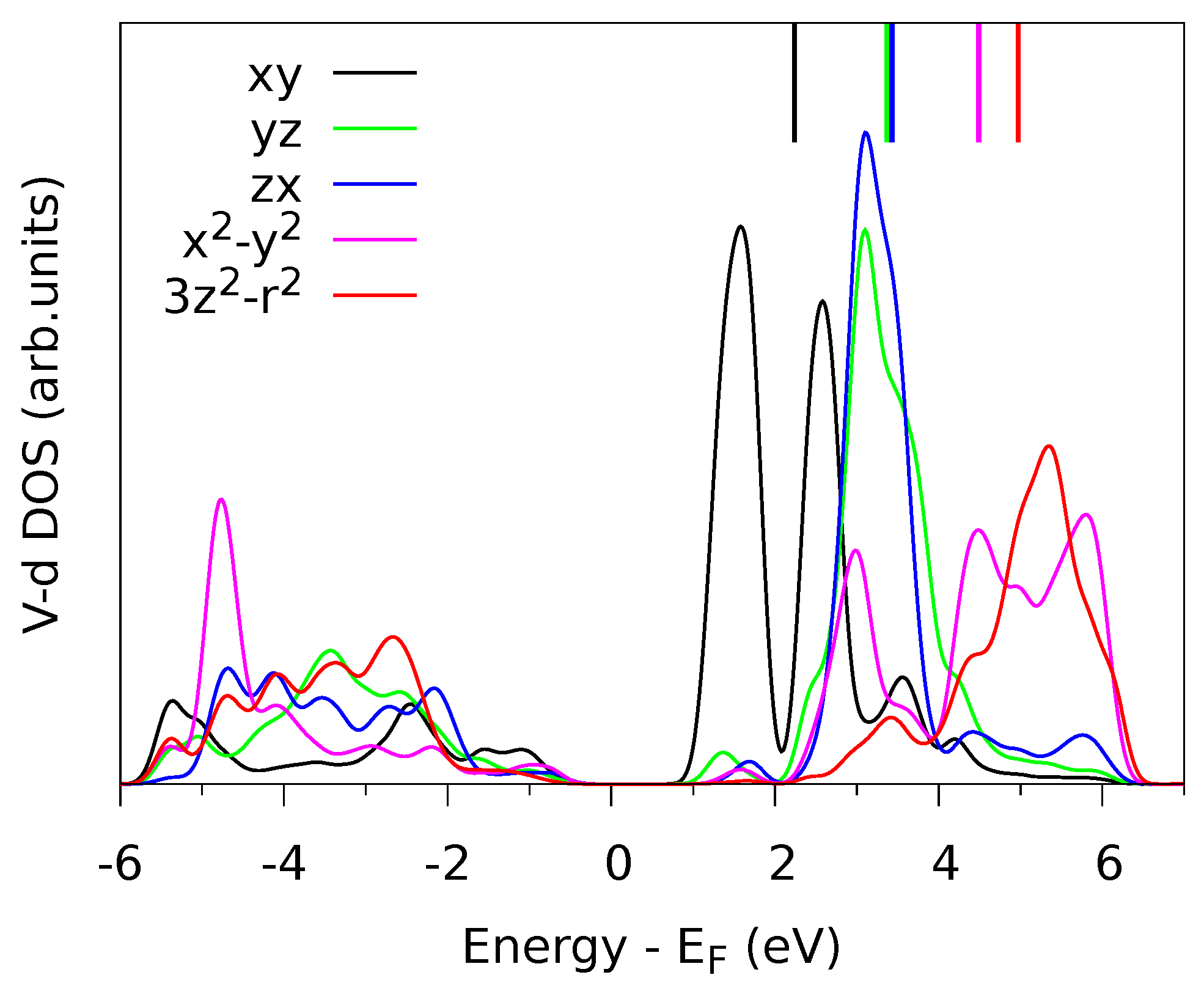The V-d partial density of states (DOS) projected onto the usual cubic d-orbitals is shown in Figure 2.

The point symmetry at the V site is very low ($C_s$) such that all five d-orbitals have a different DOS and thus a different LF energy. The point group $C_s$ has only one symmetry operation, namely the mirror $\sigma \left(y\right)$, and the d-orbitals fall into the two irreducible representations $A^{\prime }=\{3z^2-r^2, x^2-y^2, xz\}$ and $A^{″}=\{xy, yz\}$. The orbitals within each group can mix. As a consequence, the LF matrix is non-diagonal and has eight independent parameters (which excludes the average d-level energy).

For the calculation of the LF and Coulomb integral reduction factors in Equations (2)–(9), we need the eigenenergies $E_k$ and the metal d-wave amplitudes $\langle m|k\rangle$ where $|k\rangle \equiv |n\mathbf{k}\rangle$ is a band state, with $\mathbf{k}$ the crystal momentum in the first Brillouin zone and n being the band index. $E_k$ and $\langle m|k\rangle$ are directly taken from the DFT band structure (VASP PROCAR file). For the sums over k, all $\mathbf{k}$ points and the whole conduction band are used, i.e., the energy interval is 1 eV $<E_k<$ 6.5 eV (see Figure 2).

The calculated matrices N, A and $\mathsf{\Delta }$ are given in

Table 1. d-orbital projection matrix N, covalency matrix $A\equiv N^{1/2}$ and ligand field matrix $\mathsf{\Delta }$ of V${}_2$O${}_5$.

	$\mathit{xy}$	$\mathit{yz}$	$3{\mathit{z}}^2\mathbf{-}$${\mathit{r}}^2$	$\mathit{xz}$	${\mathit{x}}^2\mathbf{-}$${\mathit{y}}^2$
	0.7411	0.0064	0	0	0
	0.0064	0.6597	0	0	0
N	0	0	0.5234	0.0119	0.0027
	0	0	0.0119	0.6562	−0.0085
	0	0	0.0027	−0.0085	0.6741
	0.8608	−0.0038	0	0	0
	−0.0038	0.8122	0	0	0
A	0	0	0.7234	0.0080	−0.0008
	0	0	0.0080	0.8100	0.0051
	0	0	−0.0008	0.0051	0.8211
	2.2437	−0.0978	0	0	0
	−0.0978	3.3657	0	0	0
$\mathsf{\Delta }$	0	0	4.9664	−0.0123	−0.0008
	0	0	−0.0123	3.4269	0.1838
	0	0	−0.0008	0.1838	4.4933

. As anticipated by the symmetry analysis, there are non-zero non-diagonal matrix elements between the different orbitals of $A^{\prime }$ symmetry {$3z^2-r^2$, $xz$, $x^2-y^2$} and between those of $A^{″}$ symmetry {$xy$, $yz$}. In the present case, the non-diagonal matrix elements are small. For the covalency matrix A, the non-diagonal matrix elements are about 100 times smaller than the diagonal ones. For the LF matrix $\mathsf{\Delta }$ the non-diagonal elements are roughly 10 times smaller than the corresponding level splittings, e.g., the splitting between $xy$ and $yz$ is 1.1 eV and the non-diagonal term is 0.1 eV. We also note that the diagonal matrix elements for $yz$ and $xz$ are nearly the same. This means that, although the exact point symmetry of the metal site is $C_s$, it may be reasonable to approximate the LF using the higher symmetry group $C_{4v}$ where the d-level splits into only four sub-levels ($b_2=xy$, $e=\{xz,yz\}$, $a_1=3z^2-r^2$ and $b_1=x^2-y^2$) and there are no non-diagonal terms. Approximate point symmetries are often used in LFMT [9]. With the present method, by looking at $\mathsf{\Delta }$ and A, one can easily check whether such an approximation is valid. The five ligand field levels (diagonal matrix elements in $\mathsf{\Delta }$ of Table 1) are indicated in Figure 2 as vertical bars above the DOS plot. It can be seen that the levels correspond well to the centers of different DOS distributions.

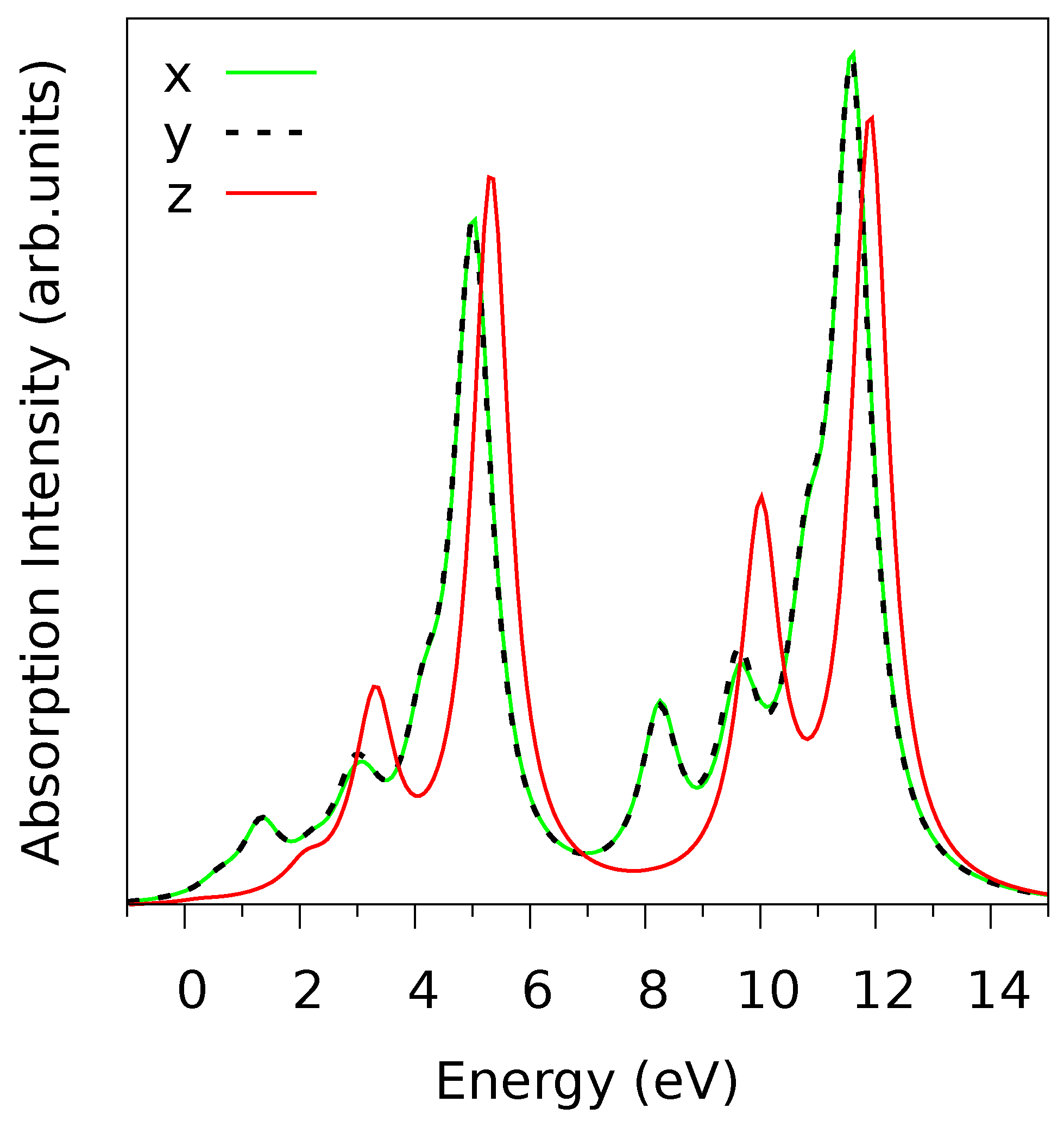
The calculated V L-edge absorption spectra for linearly polarized light along the three crystal axes are shown in Figure 3. There is only a tiny difference between the x and y polarization, which is expected from the fact that the LF has approximately $C_{4v}$ symmetry as noticed above. However, the z-polarized spectra are very different from the $x,y$-spectra, which reflects the layered structure of V${}_2$O${}_5$ and the strong anisotropy of the VO${}_6$ octahedra, due to the vanadyl bond oriented along z [15]. The ligand field energies of the five V-$3d$ orbitals increase in the order $xy$, $yz$, $zx$, $x^2-y^2$, $3z^2-r^2$; see Table 1. The finding that the $t_{2g}$-like orbitals ($xy$,$yz$,$zx$) are lower than the $e_g$-like ones ($x^2-y^2$, $3z^2-r^2$) is typical for octahedral coordination and it reflects the fact that the V-$3d$–O-$2p$ bonds of $\sigma$-type that involve the $e_g$-like d-orbitals are stronger than the $\pi$-bonds made by the $t_{2g}$-like orbitals. It is remarkable, however, that the ligand field level of $xy$ is about 1 eV lower than that of $yz$, $zx$, which suggests that the $\pi$-bonding of the $xy$-orbital is particularly weak. The $xy$-level is responsible for the lowest energy peak in the L-edge spectra (at 1 eV in Figure 3), as can be inferred from the peak energy and polarization dependence. Indeed, the fact that this peak vanishes for z-polarized light (see Figure 3) clearly indicates in-plane orientation of the orbital [15]. We also note that the $3z^2-r^2$ orbital has the largest ligand field level, which means that the antibonding molecular orbitals that are formed by the V-$3d$ and O-$2p$ states are most strongly hybridized in the case of the V $3z^2-r^2$ orbital, which makes the V=O vanadyl bond. This shows that the vanadyl bond, even though it involves only one O ligand atom, is much stronger than any other V-O bond, and even stronger than the four V-O $\sigma$ bonds that are formed by the $x^2-y^2$ orbital combined. The bond strengths of the different V-$3d$ orbitals are closely related to their covalency. We may characterize the covalency (or hybridization) of an orbital $|dm\rangle$ by the quantity $c_m=1-{\alpha }_m^2$. In the present case, where the off-diagonal elements of A are very small, we have ${\alpha }_m\approx A_{mm}$ and thus $c_m\approx 1-A_{mm}^2\approx 1-N_{mm}$. From Table 1, the $c_m$ values are: 0.26 ($xy$), 0.34 ($yz$,$xz$), 0.33 ($x^2-y^2$), 0.48 ($3z^2-r^2$). Clearly, the $xy$-orbital is the least hybridized, indicating an almost non-bonding state, while $3z^2-r^2$ is most strongly hybridized, which reflects the strongly covalent vanadyl double bond.

As explained above, the reduction of Coulomb integrals is taken into account in an orbital-dependent way. The larger the hybridization of an orbital $|dm\rangle$ (i.e., the smaller ${\alpha }_m$), the smaller is $\kappa$ in Equation (7), i.e., the stronger is the reduction of the Coulomb integrals. For example, the $2p-3d$ Coulomb integrals for the $3z^2-r^2$ orbital are reduced by 48%, while those with the $xy$-orbitals are reduced only by 26%. For the $3d-3d$ Coulomb integrals where $\kappa \propto {\alpha }^4$, the effect is even stronger [10], but in the present case of a $V^{5+}$-ion with $3d^0$ ground and $2p^{5}3d^1$ final states, the $3d-3d$ integrals do not enter the calculation. Previously we have shown that taking into account the orbital dependence of the Coulomb integrals in ligand field multiplet calculations improves the agreement of the spectra with experiments (i.e., for CoO, NiO) although the effect is rather small [10]. The oscillator strengths are also modified by the orbital-dependent covalency factors; see Equation (10). Here, this effect is taken into account for the first time. The reduction of the oscillator strength is given by $1-{\alpha }_m^2$, which is maximum for the $3z^2-r^2$-orbital (48%). This decreases the relative weight of the two dominant peaks (at ∼5 eV and ∼11.5 eV in Figure 3) and it improves agreement with experiments, as we have checked.

In Figure 4 we compare calculated spectra with experimental data [16] for p-polarized light incident at an angle of 90${}^{\circ }$ or 30${}^{\circ }$ from the surface plane. It is seen that the experimental $L_2$-peak (with maximum at 525 eV) is much broader than the $L_3$-peak (with a maximum at 518 eV). This is not uncommon for light 3d elements because the $2p_{1/2}$ hole has a shorter lifetime than the $2p_{3/2}$ hole [17]. This is partly due to the $L_2{L}_3{M}_{45}$ Auger decay, which reduces the lifetime of the $2p_{1/2}$ hole. In the case of V${}_2$O${}_5$, the fact that the oxygen K-edge (not shown) is only about 5 eV above the V-$L_2$ peak may also play a role. The near resonance between the V-$2p_{1/2}$ and the O-$1s$ core levels might induce multi-atomic decay processes that further broaden the $L_2$-peak. To account for the enhanced broadening of the $L_2$-peak in a phenomenological way, we convoluted the spectra with a Lorenzian of energy-dependent FWHM, given by $\mathsf{\Gamma }\left(E\right)=a(E-E_0)+b$, where E is the photon energy and $E_0=513.5$ eV is the absorption threshold. We take $a=0.04$, $b=0.15$ eV, such that the FWHM is 0.33 eV at the $L_3$ peak maximum and 0.61 eV at the $L_2$ maximum. A similar broadening model was successfully used for the L-edge spectra of TiO${}_2$ [18]. The reason why we use a linearly increasing FWHM rather than two fixed values for $L_2$ and $L_3$ is that for light transition element there is strong configuration mixing between the two edges [18].

In Figure 4, the calculated spectra agree very well with the experimental ones. Almost all features seen in the data are also present in the calculation, except for the weak shoulder structure in the experimental spectrum at 519 eV. The energy positions and intensities of the various peaks differ a little and the $L_2$-peak is broader in the experiment than in theory, but the overall agreement is remarkably good, in particular the differences between the 90${}^{\circ }$ and 30${}^{\circ }$ spectrum. The agreement between experiment and theory obtained here is at least as good as that obtained with quantum chemistry configuration interaction methods [16,19] and multichannel multiple scattering theory [15]. This means that parameterized LFMT can be as reliable and predictive as ab initio quantum chemistry approaches such as CAS-SCF [12] and RAS-SCF [16], if the LF parameters are computed using the present, non-empirical theory. The advantage of the present LFMT method is that it is simpler and computationally much lighter than those ab initio schemes, because we only need to perform the routine task of a DFT ground state calculation. Moreover, the present method can be applied to molecules [10] and solids in the same way. By contrast, when using quantum chemistry methods for the solid state, convergence with respect to cluster size is often a problem [16,19]. The present approach has some aspects in common with the parameterization of the LF multiplet model using Wannier functions [7,20]. The Wannier method is powerful and flexible, but more complicated than the present method, especially for the low symmetry systems considered here, where the construction of symmetry adapted Wannier functions may be challenging [21].

4. Conclusions

In summary, the recent method of non-empirical ligand field parameter determination of Ref. [10] has been generalized to systems of arbitrary symmetry. The ligand field levels and the covalency factors of the different d-orbitals become 5 × 5 matrices that have non-zero non-diagonal elements in case of low symmetry. For high symmetry, the present scheme reduces to [10]. The covalency of the d-orbitals rescales the Coulomb integrals and the oscillator strengths in an orbital-dependent way. The method has been applied to V${}_2$O${}_5$, which has a very low point symmetry ($C_s$). The calculated spectra agree very well with experiments, and the agreement is on the same level as full ab initio quantum chemistry approaches. The advantage of the present scheme is that it is computationally much simpler and that it can be easily implemented into parameterized LFMT codes, which are widely used for the analysis of L-edge spectra [3]. The present theory removes the major shortcoming of LFMT, i.e., the need for empirical parameters, while keeping its main advantages, namely conceptual simplicity and versatility at a low numerical cost.