Vector Similarity Measures of Dual Hesitant Fuzzy Linguistic Term Sets and Their Applications

Abstract

The dual hesitant fuzzy linguistic term set (DHFLTS) is defined by two functions that express the grade of membership and the grade of non-membership using a set of linguistic terms. In the present work, we first quote an example to point out that the existing complement operation of DHFLTS is on the wrong track. Meanwhile, we redefine this operation to fill the holes in the existing ones. Next, the notion of information energy under a dual hesitant fuzzy linguistic background is provided in order to build the criteria weight determination model. To further facilitate the theory of DHFLTS, we propose two vector similarity measures, i.e., Jaccard and Dice similarity measures, and their weighted forms for DHFLTS. In addition, we pioneer some generalized similarity measures of DHFLTSs and indicate that the Dice similarity measures are particular instances of the generalized similarity measures for some parameter values. Afterward, the similarity measures-based model with unknown weight information under the background of dual hesitant fuzzy linguistic environment is constructed. Lastly, an illustrated example is included to validate the method’s application, along with sensitivity analysis and comparative analysis, demonstrating the practicality and validity of its results.

1. Introduction

In everyday life, decision-making is critical to selecting the best option from a set of available options. It usually helps the experts or decision-makers (DMs) to resolve issues by evaluating alternative selections and selecting the best direction to take. An inconvenience, however, is encountered by the DMs when dealing with vague and uncertain data. By originating the concept of fuzzy set (FS), Zadeh [1] minimized the hurdles of DMs. FS has opened up new perspectives to handle the hesitation and vagueness comprised in the decision-making scheme. It has been studied at length and employed in various fields; we can see reference work [2,3,4,5,6,7,8]. In decision making, DMs evaluation information that is usually not quantitative, but rather some abstract linguistic terms. For instance, “very good”, “worst”, and “little” cannot be communicated by numerical values, but they are understandable, intuitive, and close to the cognition of individuals. As a result, Zadeh (1975) used linguistic variables to represent ambiguous data. The authors in [9,10] constructed group decision consensus frameworks under the background of linguistic evaluation information. Xu [11] extended the notion of linguistic variables to uncertain linguistic variables and designed several uncertain linguistic aggregation operators to be applied in multi-criteria group decision-making (MCGDM). Xian et al. [12,13] introduced a range of fuzzy linguistic operators and discussed their applications in group decision-making.

Because of the uncertainty of the practical problems, a sole linguistic variable cannot capture the hesitancy of DMs appropriately. Therefore, Rodriguez et al. [14] devised hesitant fuzzy linguistic term sets (HFLTSs) to state the precedence of DMs by coupling hesitant fuzzy sets (HFSs) [15] and linguistic term sets (LTSs) [16]. Since the introduction of HFLTS, numerous methods have been studied and applied to MCDM problems. However, HFLTS has inadequate information because it only considers membership values but ignores non-membership values. To circumvent this drawback, Yang and Ju [17] developed a more accurate and precise tool, namely the dual hesitant fuzzy linguistic term set (DHFLTS). DHFLTS takes more information, owing to which it can be deemed a more generalized set that supports a more flexible framework when the DMs express their opinions. Yang and Ju [17] studied the relevant operational laws, the comparative method, and a series of aggregation operators. Qu et al. [18] paid attention to regret theory and structured an MCDM model for hesitant fuzzy linguistic environments as well as dual hesitant fuzzy linguistic environments with unknown weight information.

Similarity and distance measures are broadly used to establish the relationship between two individuals in many domains [19,20,21,22,23], in particular medical diagnosis, pattern recognition, engineering, and network comparison. The “classical” similarity measures contain the cosine formula, Jaccard’s measure, Dice’s measure, overlap measures, and the correlation coefficient of Pearson [24]. Jaccard, Dice, and cosine measures are sorts of vector similarity measures. With the origination of FSs, “classical” similarity measures have been extended to countless fuzzy contexts [25,26,27,28,29,30]. Liu et al. [20] presented a technique for order of preference by similarity to the ideal solution (TOPSIS) model for q-rung orthopair fuzzy sets according to their diagnosed cosine similarity measures. Beg and Ashraf conducted an in-depth study regarding the numerous features of similarity measures under the background of FSs [31]. Ye [32] probed Jaccard, Dice, and cosine similarity measures to HFSs. Ye and Jun [33] examined the generalized Dice similarity measures between simplified neutrosophic sets and established the generalized Dice measures-based MCDM approach with simplified neutrosophic information. Ejegwa [34] presented several axiomatic definitions of Pythagorean fuzzy distance and similarity measures and delineated their characteristics in-depth. To improve the existing similarity measures for picture fuzzy sets (PFSs), Singh and Ganie [28] put forward some novel similarity measures and discussed their applications in pattern recognition. Singh and his coworker Kumar [29] investigated some advanced similarity measures for IFSs and built a model for face recognition problems utilizing the developed measures. Song and Hu [35] developed two similarity measures for HFLTSs and used them to MCDM issues. The authors in [36] came up with some weighted Dice similarity measures and weighted generalized Dice similarity for probabilistic uncertain linguistic environment and applied them in finding the optimal location of the electric vehicle. A study by Zhang et al. [37] put forward various innovative hesitant fuzzy linguistic similarity measures and explored their properties at length. Recently, Verma [38] pioneered various linguistic q-rung orthopair fuzzy trigonometric similarity measures based on linguistic scale function and discussed their application in decision-making problems. However, these existing similarity measures cannot be utilized to assess the degree of similarity between two DHFLTS. Though in a number of practical scenarios, DMs prefer to convey their assessment information in terms of a dual hesitant fuzzy linguistic context, bearing in mind the dual nature of the context, i.e., its qualitative and quantitative aspects. It is worth noting that most of the aforementioned FSs are special cases of DHFLTS:

(i)

If the linguistic component is removed, the DHFLTS, i.e., Equation (1), is converted to DHFS, which is $\left\{〈g(ɲ),h(ɲ)〉|ɲ\in X\right\}.$

(ii)

If the linguistic and non-membership components are removed, the DHFLTS, i.e., Equation (1), is converted to HFS, which is $\left\{〈g(ɲ)〉|ɲ\in X\right\}.$

(iii)

If the linguistic component is removed and the membership and non-membership parts are reduced to a single value, the DHFLTS, i.e., Equation (1), is converted to IFS, which is $\left\{〈\alpha (ɲ),\beta (ɲ)〉|ɲ\in X\right\}.$

Thus, the DHFLTS theory is an effective way to deal with qualitative and uncertain information in real-world circumstances. Moreover, the Jaccard and Dice similarity measures are simple and modest tools for quantifying the degree of similarity between two choices. However, these have not been investigated using the DHFLTS framework. Therefore, expanding these measures to dual hesitant fuzzy linguistic contexts is essential to meet the requirements of DMs’ preference and flexible decision-making. This inspired us to address the issues caused by the setting of DHFLTSs. It is worth noting that decision-making in the context of DHFLTS may receive greater attention and merit wider acknowledgment and additional research.

Entropy is a key concept for measuring uncertainty in fuzzy information. There has been a lot of research carried out on entropy measurements for FSs [39], intuitionistic fuzzy sets (IFSs) [40] and HFSs [41,42]. It is mainly used to measure the uncertainty level of fuzzy information and can be used to derive the weight of each criteria under incomplete information. Hung and Chen [43] offered a TOPSIS model utilizing entropy weight to address MCDM problems under an intuitionistic fuzzy setting. Zou et al. [44] introduced a novel weight determination method based on the entropy measure and applied it to water quality assessment. Ye studied a decision-making algorithm in accordance with weighted correlation coefficients utilizing entropy weights under the background of interval-valued intuitionistic fuzzy sets for some cases where the detail about the criteria weights is completely unknown. To treat both cases of criteria weights, i.e., when the detail about the weights is fully unknown or partly known, Liu and Ren [45] presented two models: one is the expansion of the ordinary entropy weight model, and the other is an optimal model based on the proposed intuitionistic fuzzy entropy measure. Liu et al. [46] paid attention to evidential theory and built a double hierarchy hesitant fuzzy linguistic entropy-based TODIM approach. Recently, Aggarwal [47] studied different fuzzy entropy functions with different ranges of values and expanded to the probabilistic-fuzzy domain. Farhadinia and Xu [48] established a range of entropies for HFLTSs by utilizing the arithmetic mean of entropies for single linguistic terms in an HFLTS. Gou et al. [49] outlined the entropy measures of an HFLTS founded on the similarity degree and its negation. Scholars have made numerous other accomplishments on this topic for various fuzzy environments, but to the best of our knowledge, no such study on dual hesitant fuzzy linguistic context exists. Thus, there is a need to present the notion of entropy measure and the corresponding entropy-weight determination model for the DHFLTS, which is a comprehensive set that reflects both the membership and non-membership values of the HFLTS.

The main objectives of the current study are outlined as follows:

• To redefine the complement operation of DHFLTS in order to fulfill the disadvantages of the existing one [18]. The details of the disadvantages can be found in Section 2.2.
• To present dual hesitant fuzzy linguistic Jaccard similarity measures, Dice similarity measures, and their weighted forms. To this end, there is no need to add a linguistic term to shorter DHFLTS to have the same number of linguistic terms in both DHFLTS, so the result is more accurate because the information is not distorted.
• To propose the generalized Dice similarity measures of DHFLTS and their characteristics, along with proof.
• To develop an approach by applying the proposed entropy formula to calculate the weight vector of criteria.
• To construct the similarity measures-based MCDM model with dual hesitant fuzzy linguistic information.

The framework of this study is arranged as follows: In Section 2, some basic concepts regarding DHFLTS are introduced. Section 3 proposes the Jaccard and Dice similarity measure, weighted Jaccard and Dice similarity measures, and generalized Jaccard and Dice similarity measures under the background of DHFLTS. Section 4 presents the paper’s key contribution and constructs the MCDM model based on the devised similarity measures with fully unknown weight information. In Section 5, an illustrated example is provided to demonstrate the applicability of the proffered work. Section 6 provides a comparative analysis to analyze the results of the schemed model. Finally, Section 7 concludes the article with some concluding remarks.

2. Preliminary Knowledge

To facilitate the coming discussion, some basic definitions related to LTS and DHFLTS are recalled in this part.

2.1. Linguistic Term Set

Let $S=\left\{{\upharpoonleft }_0,{\upharpoonleft }_1,\dots ,{\upharpoonleft }_l\right\}$ be an LTS with odd cardinality, where $s_j$ presents a possible value for a linguistic variable, $l+1$ is the cardinality of S. Take for example, $l=6$, a set of seven terms S could be formed as given below: $S=\left\{{\upharpoonleft }_0=\mathrm{extremely}\mathrm{poor},{\upharpoonleft }_1=\mathrm{very}\mathrm{poor},{\upharpoonleft }_2=\mathrm{poor},{\upharpoonleft }_3=\mathrm{medium},{\upharpoonleft }_4=\mathrm{good},\right.\left.{\upharpoonleft }_3=\mathrm{medium},{\upharpoonleft }_4=\mathrm{good},{\upharpoonleft }_5=\mathrm{very}\mathrm{good},{\upharpoonleft }_6=\mathrm{extremely}\mathrm{good}\right\}.$

Generally, any linguistic term set S should meet the following properties [9,50]:

• The set is ordered: ${\upharpoonleft }_j>{\upharpoonleft }_i,$ if and only if $j>i;$
• Negation operator: $Neg\left({\upharpoonleft }_j\right)={\upharpoonleft }_i,$ such that $i=l-j;$
• Maximum operator: $max\left({\upharpoonleft }_j,{\upharpoonleft }_i\right)={\upharpoonleft }_j,$ if $j>i;$
• Minimum operator: $min\left({\upharpoonleft }_j,{\upharpoonleft }_i\right)={\upharpoonleft }_i,$ if $j>i.$

2.2. Dual Hesitant Fuzzy Linguistic Term Set

Definition 1 

([17]). Let X be a universe of discourse, then a dual hesitant fuzzy linguistic term set (DHFLTS) on X is described as:

$$D=\left\{〈ɲ,S_{\vartheta (ɲ)},g(ɲ),h(ɲ)〉|ɲ\in X\right\},$$

(1)

where ${\upharpoonleft }_{\vartheta (ɲ)}\in S=\left\{{\upharpoonleft }_0,{\upharpoonleft }_1,\dots ,{\upharpoonleft }_l\right\},$$g(ɲ)$ and $h(ɲ)$ are subsets of some values in $\left[0,1\right],$ presenting the possible membership grades and non-membership grades of the element $ɲ\in X$ to the linguistic variable ${\upharpoonleft }_{\vartheta (ɲ)}$, respectively, with the conditions: $0\le \alpha ,\beta \le 1,0\le {\alpha }^{+}+{\beta }^{+}\le 1,$ where $\alpha \in g(ɲ),\beta \in h(ɲ),{\alpha }^{+}=\mathrm{supremum}\left(g(ɲ)\right),$ and ${\beta }^{+}=\mathrm{supremum}\left(h(ɲ)\right)\forall ɲ\in X.$ For convince, the pair $d(ɲ)=〈{\upharpoonleft }_{\vartheta (ɲ)},g(ɲ),h(ɲ)〉$ is called a dual hesitant fuzzy linguistic element (DHFLE) marked by $d=〈{\upharpoonleft }_{\vartheta },g,h〉.$

Some special DHFLEs are:

• Complete certainty DHFLE: $d=\left\{{\upharpoonleft }_j,\left\{1\right\},\left\{0\right\}\right\};$
• Complete uncertainty DHFLE: $d=\left\{{\upharpoonleft }_j,\left\{0\right\},\left\{1\right\}\right\};$
• Empty DHFLE: $d=\varphi .$

For normalization purposes, Qu et al. [18] gave the complement of DHFLE as given below.

Definition 2. 

The complement of DHFLE, $d=〈{\upharpoonleft }_{\vartheta (ɲ)},g,h〉$, is defined as:

$$d^c=〈{\upharpoonleft }_{l-\vartheta (ɲ)},\tilde{g},\tilde{h}〉,$$

(2)

where $\tilde{g}={\displaystyle \bigcup _{\alpha \in g}}\left\{1-\alpha \right\},$$\tilde{h}={\displaystyle \bigcup _{\beta \in h}}\left\{1-\beta \right\},$$l+1$ is the cardinality of S.

In what follows, we first give some critical examples in order to disclose that the complement operation given by [18] is invalid. After this, we shall redefine this operation to handle the MCGDM problem (involving cost criteria) accurately.

To justify the invalidity of the existing dual hesitant fuzzy linguistic operation, we provide the following example:

Example 1. 

Consider the DHFLES $d_1=\left\{{\upharpoonleft }_3,\left\{0.4,0.6\right\},\left\{0.3,0.4\right\}\right\},$ $d_2=\left\{{\upharpoonleft }_2,\left\{0.2,0.3,0.4\right\},\right.\left.\left\{0.3,0.5\right\}\right\},$ using the linguistic term set $S=\left\{{\upharpoonleft }_0=\mathit{extremely}\mathit{low},{\upharpoonleft }_1=\mathit{very}\mathit{low},{\upharpoonleft }_2=\mathit{low},\right.\left.{\upharpoonleft }_3=\mathit{medium},{\upharpoonleft }_4=\mathit{high},{\upharpoonleft }_5=\mathit{very}\mathit{high},{\upharpoonleft }_6=\mathit{extremely}\mathit{high}\right\}.$

According to Equation (3), we have $d_1^c=\left\{{\upharpoonleft }_3,\left\{0.6,0.4\right\},\left\{0.7,0.6\right\}\right\},$ and $d_2^c=\left\{{\upharpoonleft }_4,\right.\left.\left\{0.8,0.7,0.6\right\},\left\{0.7,0.5\right\}\right\}.$ For $d_1^c$, ${\alpha }^{+}=0.6$ and ${\beta }^{+}=0.7$ whose sum is $1.3>1$. Thus, $d_1^c$ does not satisfy the condition of DHFLTS. Similarly, for $d_2^c$ we have ${\alpha }^{+}+{\beta }^{+}=1.5>1.$ Therefore, $d_1^c$ and $d_2^c$ are no longer DHFLTSs.

From the above examples, it is clear that Equation (3) is off-target and will lead to bogus results, especially when cost-type criteria are involved in the problem.

Definition 3. 

The complement of DHFLE, $d=〈{\upharpoonleft }_{\vartheta (ɲ)},g,h〉$, is defined as:

$$d^c=〈{\upharpoonleft }_{l-\vartheta (ɲ)},h,g〉,$$

(3)

here $l+1$ is the cardinality of S.

Proposition 1. 

The complement of d is involutive.

The information measure has not been deployed for DHFLTSs in past studies. In order to enrich the theoretical basis of DHFLTSs and promote their widespread use in a variety of disciplines, their formulation is inevitable.

Inspired by the information energy given by [51], in the following, we put forward this concept for original DHFLTS [17].

Definition 4. 

The information energy of DHFLTS ‘D’ is defined as:

$$E\left(D\right)={\displaystyle \sum _{j=1}^m}\left(\frac{1}{\#g\left(d_j\right)}{\displaystyle \sum _{ı=1}^{\#g\left(d_j\right)}}{\alpha }_{ı}^2\left(d_j\right){\left(\frac{\vartheta \left(d_j\right)}{l}\right)}^2+\frac{1}{\#h\left(d_j\right)}{\displaystyle \sum _{ı=1}^{\#h\left(d_j\right)}}{\beta }_{ı}^2\left(d_j\right){\left(\frac{\vartheta \left(d_j\right)}{l}\right)}^2\right),$$

(4)

here, ‘$\#g\left(d_j\right)$’ and ‘$\#h\left(d_j\right)$’ present the number of elements in ‘${\alpha }_{ı}$’ and ‘${\beta }_{ı}$’, respectively, and ‘m’ is the cardinality of X.

Definition 5 

([17]). Let $d_1=〈{\upharpoonleft }_{{\vartheta }_1},g_1,h_1〉$ and $d_2=〈{\upharpoonleft }_{{\vartheta }_2},g_2,h_2〉$ be two DHFLEs, then the governing operational rules are given as:

1. 

$d_1\oplus d_2=〈{\upharpoonleft }_{{\vartheta }_1+{\vartheta }_2},\left\{{\displaystyle \bigcup _{\begin{array}{c}{\alpha }_1\in g_1,\\ {\alpha }_2\in g_2\end{array}}}\left\{{\alpha }_1+{\alpha }_2-{\alpha }_1{\alpha }_2\right\},{\displaystyle \bigcup _{\begin{array}{c}{\beta }_1\in h_1,\\ {\beta }_2\in h_2\end{array}}}\left\{{\beta }_1{\beta }_2\right\}\right\}〉;$

2. 

$d_1\otimes d_2=〈{\upharpoonleft }_{{\vartheta }_1\times {\vartheta }_2},\left\{{\displaystyle \bigcup _{\begin{array}{c}{\alpha }_1\in g_1,\\ {\alpha }_2\in g_2\end{array}}}\left\{{\alpha }_1{\alpha }_2\right\},{\bigcup }_{\begin{array}{c}{\beta }_1\in h_1,\\ {\beta }_2\in h_2\end{array}}\left\{{\beta }_1+{\beta }_2-{\beta }_1{\beta }_2\right\}\right\}〉;$

3. 

$\eta d_1=〈{\upharpoonleft }_{\eta {\vartheta }_1},\left\{{\displaystyle \bigcup _{{\alpha }_1\in g_1}}\left\{1-{\left(1-{\alpha }_1\right)}^{\eta }\right\},{\displaystyle \bigcup _{{\beta }_1\in h_1}}\left\{{\left({\beta }_1\right)}^{\eta }\right\}\right\}〉,\eta >0;$

4. 

$d_1^{\eta }=〈{\upharpoonleft }_{{\vartheta }_1^{\eta }},\left\{{\displaystyle \bigcup _{{\alpha }_1\in g_1}}\left\{{\left({\alpha }_1\right)}^{\eta }\right\},{\displaystyle \bigcup _{{\beta }_1\in h_1}}\left\{1-{\left(1-{\beta }_1\right)}^{\eta }\right\}\right\}〉,\eta >0.$

Definition 6 

([17]). Let $d=〈{\upharpoonleft }_{\vartheta },g,h〉$ be a DHFE, then the score function $Sco\left(d\right)$ and the accuracy function $Acc\left(d\right)$ of d are given by

$$Sco\left(d\right)=\frac{\vartheta }{l}\times \left(\frac{1}{\#g}{\displaystyle \sum _{\alpha \in g}^{}}\alpha -\frac{1}{\#h}{\displaystyle \sum _{\beta \in h}^{}}\beta \right),$$

(5)

$$Acc\left(d\right)=\frac{\vartheta }{l}\times \left(\frac{1}{\#g}{\displaystyle \sum _{\alpha \in g}^{}}\alpha +\frac{1}{\#h}{\displaystyle \sum _{\beta \in h}^{}}\beta \right),$$

(6)

where $\#g$ and $\#h$ denote the number of values in g and h, respectively, $\left(l+1\right)$ is the cardinality of $S=\left\{{\upharpoonleft }_0,{\upharpoonleft }_1,\dots ,{\upharpoonleft }_l\right\}.$

Definition 7. 

Let $d_1=〈{\upharpoonleft }_{{\vartheta }_1},g_1,h_1〉$ and $d_2=〈{\upharpoonleft }_{{\vartheta }_2},g_2,h_2〉$ be any two DHFLEs, then they can be compared using the following laws:

(1). 

If $Sco\left(d_1\right)>Sco\left(d_2\right),$ then $d_1\succ d_2$;

(2). 

If $Sco\left(d_1\right)=Sco\left(d_2\right),$ then:

(i). 

if $Acc\left(d_1\right)>Acc\left(d_2\right),$ then $d_1\prec d_2$;

(ii). 

if $Acc\left(d_1\right)=Acc\left(d_2\right),$ then $d_1=d_2.$

Definition 8 

([18]). Let $d=〈{\upharpoonleft }_{\vartheta },g,h〉$ be a DHFLE, then its average deviation function $\sigma \left(d\right)$ is given by

$$\sigma \left(d\right)=\frac{1}{\#g}{\displaystyle \sum _{\alpha \in g}^{}}\left|\frac{\vartheta }{l}\alpha -Sco\left(d\right)\right|+\frac{1}{\#h}{\displaystyle \sum _{\beta \in h}^{}}\left|\frac{\vartheta }{l}\beta -Sco\left(d\right)\right|,$$

(7)

where $\#g$ and $\#h$ denote the number of values in g and h, respectively, $\left(l+1\right)$ is the cardinality of $S=\left\{{\upharpoonleft }_0,{\upharpoonleft }_1,\dots ,{\upharpoonleft }_l\right\}.$

2.3. Classical Vector Similarity Measures

In the following, we present the definition of two classical vector similarity measures: Jaccard similarity [52] and Dice similarity [53].

Definition 9. 

Let $U=\left\{u_1,u_2,\dots ,u_n\right\}$ and $V=\left\{v_1,v_2,\dots ,v_n\right\}$ be two positive vectors of length n. Then the Jaccard $\mathcal{J}\left(U,V\right)$ and Dice $\mathcal{D}\left(U,V\right)$ similarity measures are stated as follows:

$$\begin{array}{cc}\hfill \mathcal{J}\left(U,V\right)& =\frac{U·V}{{\left|\left|U\right|\right|}_2^2+{\left|\left|V\right|\right|}_2^2-U·V}\hfill \\ \hfill & =\frac{2{\displaystyle {\displaystyle \sum _{ı=1}^n}}{u}_{ı}{v}_{ı}}{{\displaystyle {\displaystyle \sum _{ı=1}^n}}{u}_{ı}^2+{\displaystyle {\displaystyle \sum _{ı=1}^n}}{v}_{ı}^2-{\displaystyle {\displaystyle \sum _{ı=1}^n}}{u}_{ı}{v}_{ı}},\hfill \end{array}$$

(8)

$$\begin{array}{cc}\hfill \mathcal{D}\left(U,V\right)& =\frac{2U·V}{{\left|\left|U\right|\right|}_2^2+{\left|\left|V\right|\right|}_2^2}\hfill \\ \hfill & =\frac{2{\displaystyle {\displaystyle \sum _{ı=1}^n}}{u}_{ı}{v}_{ı}}{{\displaystyle {\displaystyle \sum _{ı=1}^n}}{u}_{ı}^2+{\displaystyle {\displaystyle \sum _{ı=1}^n}}{v}_{ı}^2},\hfill \end{array}$$

(9)

where $U·V={\displaystyle {\displaystyle \sum _{ı=1}^n}}{u}_{ı}{v}_{ı}$ is the inner product of U and V and ${\left|\left|U\right|\right|}_2=\sqrt{{\displaystyle {\displaystyle \sum _{ı=1}^n}}{u}_{ı}^2}$ and ${\left|\left|V\right|\right|}_2=\sqrt{{\displaystyle {\displaystyle \sum _{ı=1}^n}}{v}_{ı}^2}$ are the Euclidean norms of U and V( also called the $L_2$ norms).

3. Vector Similarity Measures with Dual Hesitant Fuzzy Linguistic Information

Similarity measure is an important topic in pattern recognition and medical diagnosis areas. In the following, we introduce Jaccard similarity measure and Dice similarity measures between DHFLTSs.

3.1. Jaccard and Dice Similarity Measures for DHFLTSs

Definition 10. 

Let $S=\left\{{\upharpoonleft }_0,{\upharpoonleft }_1,\dots ,{\upharpoonleft }_l\right\}$ be an LTS. For two DHFLTSs $D_1=\left\{〈{ɲ}_i,{\upharpoonleft }_{\vartheta \left({ɲ}_i\right)},g\left({ɲ}_i\right),h\left({ɲ}_i\right)〉\right.\left.|{ɲ}_i\in X\right\}$ and $D_2=\left\{〈{ɲ}_i,{\upharpoonleft }_{\overline{\vartheta }\left({ɲ}_i\right)},\overline{g}\left({ɲ}_i\right),\overline{h}\left({ɲ}_i\right)〉|{ɲ}_i\in X\right\}$, then the Jaccard ${\mathcal{J}}^1\left(D_1,D_2\right)$ similarity measures is stated as follows:

$${\mathcal{J}}^1\left(D_1,D_2\right)=\frac{1}{3n}{\displaystyle \sum _{i=1}^n}\left(\begin{array}{c}\frac{\vartheta \left({ɲ}_i\right)·\overline{\vartheta }\left({ɲ}_i\right)}{{\left(\vartheta \left({ɲ}_i\right)\right)}^2+{\left(\overline{\vartheta }\left({ɲ}_i\right)\right)}^2-\vartheta \left({ɲ}_i\right)·\overline{\vartheta }\left({ɲ}_i\right)}+\\ \frac{{\displaystyle {\displaystyle \sum _{ı=1}^{\#g}}}{\alpha }_{ı}\left({ɲ}_i\right)/\#g·{\displaystyle {\displaystyle \sum _{ı=1}^{\#\overline{g}}}}\overline{{\alpha }_{ı}}\left({ɲ}_i\right)/\#\overline{g}}{{\displaystyle {\displaystyle \sum _{ı=1}^{\#g}}}{\alpha }_{ı}^2\left({ɲ}_i\right)/\#g+{\displaystyle {\displaystyle \sum _{ı=1}^{\#\overline{g}}}}{\overline{{\alpha }_{ı}}}^2\left({ɲ}_i\right)/\#\overline{g}-{\displaystyle {\displaystyle \sum _{ı=1}^{\#g}}}{\alpha }_{ı}\left({ɲ}_i\right)/\#g·{\displaystyle {\displaystyle \sum _{ı=1}^{\#\overline{g}}}}\overline{{\alpha }_{ı}}\left({ɲ}_i\right)/\#\overline{g}}+\\ \frac{{\displaystyle \sum _{ı=1}^{\#h}}{\beta }_{ı}\left({ɲ}_i\right)/\#h·{\displaystyle \sum _{ı=1}^{\#\overline{h}}}\overline{{\beta }_{ı}}\left({ɲ}_i\right)/\#\overline{h}}{{\displaystyle {\displaystyle \sum _{ı=1}^{\#h}}}{\beta }_{ı}^2\left({ɲ}_i\right)/\#h+{\displaystyle {\displaystyle \sum _{ı=1}^{\#\overline{h}}}}{\overline{{\beta }_{ı}}}^2\left({ɲ}_i\right)/\#\overline{h}-{\displaystyle {\displaystyle \sum _{ı=1}^{\#h}}}{\beta }_{ı}\left({ɲ}_i\right)/\#h·{\displaystyle {\displaystyle \sum _{ı=1}^{\#\overline{h}}}}\overline{{\beta }_{ı}}\left({ɲ}_i\right)/\#\overline{h}}\end{array}\right),$$

(10)

Definition 11. 

Let $S=\left\{{\upharpoonleft }_0,{\upharpoonleft }_1,...,{\upharpoonleft }_l\right\}$ be an LTS. For two DHFLTSs $D_1=\left\{〈{ɲ}_i,{\upharpoonleft }_{\vartheta \left({ɲ}_i\right)},g\left({ɲ}_i\right),h\left({ɲ}_i\right)〉\right.\left.|{ɲ}_i\in X\right\}$ and $D_2=\left\{〈{ɲ}_i,{\upharpoonleft }_{\overline{\vartheta }\left({ɲ}_i\right)},\overline{g}\left({ɲ}_i\right),\overline{h}\left({ɲ}_i\right)〉|{ɲ}_i\in X\right\}$, then the Dice ${\mathcal{D}}^1\left(D_1,D_2\right)$ similarity measure is defined as follows:

$${\mathcal{D}}^1\left(D_1,D_2\right)=\frac{2}{3n}{\displaystyle \sum _{i=1}^n}\left(\begin{array}{c}\frac{\vartheta \left({ɲ}_i\right)·\overline{\vartheta }\left({ɲ}_i\right)}{{\left(\vartheta \left({ɲ}_i\right)\right)}^2+{\left(\overline{\vartheta }\left({ɲ}_i\right)\right)}^2}+\frac{{\displaystyle {\displaystyle \sum _{ı=1}^{\#g}}}{\alpha }_{ı}\left({ɲ}_i\right)/\#g·{\displaystyle {\displaystyle \sum _{ı=1}^{\#\overline{g}}}}\overline{{\alpha }_{ı}}\left({ɲ}_i\right)/\#\overline{g}}{{\displaystyle {\displaystyle \sum _{ı=1}^{\#g}}}{\alpha }_{ı}^2\left({ɲ}_i\right)/\#g+{\displaystyle {\displaystyle \sum _{ı=1}^{\#\overline{g}}}}{\overline{{\alpha }_{ı}}}^2\left({ɲ}_i\right)/\#\overline{g}}+\\ \frac{{\displaystyle {\displaystyle \sum _{ı=1}^{\#h}}}{\beta }_{ı}\left({ɲ}_i\right)/\#h·{\displaystyle {\displaystyle \sum _{ı=1}^{\#\overline{h}}}}\overline{{\beta }_{ı}}\left({ɲ}_i\right)/\#\overline{h}}{{\displaystyle {\displaystyle \sum _{ı=1}^{\#h}}}{\beta }_{ı}^2\left({ɲ}_i\right)/\#h+{\displaystyle \sum _{ı=1}^{\#\overline{h}}}{\overline{{\beta }_{ı}}}^2\left({ɲ}_i\right)/\#\overline{h}}\end{array}\right),$$

(11)

Some theorems of Jaccard ${\mathcal{J}}^1\left(D_1,D_2\right)$ and Dice ${\mathcal{D}}^1\left(D_1,D_2\right)$ similarity measures are given below.

Theorem 1. 

The Jaccard similarity measure ${\mathcal{J}}^1\left(D_1,D_2\right)$ between two DHFLTSs, $D_1$ and $D_2$, possesses the following characteristics:

1. 

${\mathcal{J}}^1\left(D_1,D_2\right)={\mathcal{J}}^1\left(D_2,D_1\right);$

2. 

${\mathcal{J}}^1\left(D_1,D_2\right)=1,$ if and only if $D_1=D_2;$

3. 

$0\le {\mathcal{J}}^1\left(D_1,D_2\right)\le 1.$

Proof. 

(1) and (2) are obvious.

(3) It is evident that ${\mathcal{D}}^1\left(D_1,D_2\right)\ge 0$. According to the inequality ${ɲ}^2+{\mathit{y}}^2-ɲ\mathit{y}\ge ɲ\mathit{y}$, we have

$${\left(\vartheta \left({ɲ}_i\right)\right)}^2+{\left(\overline{\vartheta }\left({ɲ}_i\right)\right)}^2-\vartheta \left({ɲ}_i\right)\overline{\vartheta }\left({ɲ}_i\right)\ge \vartheta \left({ɲ}_i\right)\overline{\vartheta }\left({ɲ}_i\right)$$

$$⟹\frac{\vartheta \left({ɲ}_i\right)\overline{\vartheta }\left({ɲ}_i\right)}{{\left(\vartheta \left({ɲ}_i\right)\right)}^2+{\left(\overline{\vartheta }\left({ɲ}_i\right)\right)}^2-\vartheta \left({ɲ}_i\right)\overline{\vartheta }\left({ɲ}_i\right)}\le 1.$$

(12)

Similarly,

$$\frac{{\displaystyle {\displaystyle \sum _{ı=1}^{\#g}}}{\alpha }_{ı}\left({ɲ}_i\right)/\#g·{\displaystyle {\displaystyle \sum _{ı=1}^{\#\overline{g}}}}\overline{{\alpha }_{ı}}\left({ɲ}_i\right)/\#\overline{g}}{{\displaystyle {\displaystyle \sum _{ı=1}^{\#g}}}{\alpha }_{ı}^2\left({ɲ}_i\right)/\#g+{\displaystyle {\displaystyle \sum _{ı=1}^{\#\overline{g}}}}{\overline{{\alpha }_{ı}}}^2\left({ɲ}_i\right)/\#\overline{g}-{\displaystyle {\displaystyle \sum _{ı=1}^{\#g}}}{\alpha }_{ı}\left({ɲ}_i\right)/\#g·{\displaystyle {\displaystyle \sum _{ı=1}^{\#\overline{g}}}}\overline{{\alpha }_{ı}}\left({ɲ}_i\right)/\#\overline{g}}\le 1,$$

(13)

and

$$\frac{{\displaystyle {\displaystyle \sum _{ı=1}^{\#h}}}{\beta }_{ı}\left({ɲ}_i\right)/\#h·{\displaystyle {\displaystyle \sum _{ı=1}^{\#\overline{h}}}}\overline{{\beta }_{ı}}\left({ɲ}_i\right)/\#\overline{h}}{{\displaystyle {\displaystyle \sum _{ı=1}^{\#h}}}{\beta }_{ı}^2\left({ɲ}_i\right)/\#h+{\displaystyle {\displaystyle \sum _{ı=1}^{\#\overline{h}}}}{\overline{{\beta }_{ı}}}^2\left({ɲ}_i\right)/\#\overline{h}-{\displaystyle {\displaystyle \sum _{ı=1}^{\#h}}}{\beta }_{ı}\left({ɲ}_i\right)/\#h·{\displaystyle {\displaystyle \sum _{ı=1}^{\#\overline{h}}}}\overline{{\beta }_{ı}}\left({ɲ}_i\right)/\#\overline{h}}\le 1.$$

(14)

Adding Equations (12)–(14), we obtain

$$\begin{array}{cc}\hfill & \frac{\vartheta \left({ɲ}_i\right)·\overline{\vartheta }\left({ɲ}_i\right)}{{\left(\vartheta \left({ɲ}_i\right)\right)}^2+{\left(\overline{\vartheta }\left({ɲ}_i\right)\right)}^2-\vartheta \left({ɲ}_i\right)·\overline{\vartheta }\left({ɲ}_i\right)}+\frac{{\displaystyle {\displaystyle \sum _{ı=1}^{\#g}}}{\alpha }_{ı}\left({ɲ}_i\right)/\#g·{\displaystyle {\displaystyle \sum _{ı=1}^{\#\overline{g}}}}\overline{{\alpha }_{ı}}\left({ɲ}_i\right)/\#\overline{g}}{{\displaystyle {\displaystyle \sum _{ı=1}^{\#g}}}{\alpha }_{ı}^2\left({ɲ}_i\right)/\#g+{\displaystyle {\displaystyle \sum _{ı=1}^{\#\overline{g}}}}{\overline{{\alpha }_{ı}}}^2\left({ɲ}_i\right)/\#\overline{g}-{\displaystyle {\displaystyle \sum _{ı=1}^{\#g}}}{\alpha }_{ı}\left({ɲ}_i\right)/\#g·{\displaystyle {\displaystyle \sum _{ı=1}^{\#\overline{g}}}}\overline{{\alpha }_{ı}}\left({ɲ}_i\right)/\#\overline{g}}+\hfill \\ \hfill & \frac{{\displaystyle {\displaystyle \sum _{ı=1}^{\#h}}}{\beta }_{ı}\left({ɲ}_i\right)/\#h·{\displaystyle {\displaystyle \sum _{ı=1}^{\#\overline{h}}}}\overline{{\beta }_{ı}}\left({ɲ}_i\right)/\#\overline{h}}{{\displaystyle {\displaystyle \sum _{ı=1}^{\#h}}}{\beta }_{ı}^2\left({ɲ}_i\right)/\#h+{\displaystyle {\displaystyle \sum _{ı=1}^{\#\overline{h}}}}{\overline{{\beta }_{ı}}}^2\left({ɲ}_i\right)/\#\overline{h}-{\displaystyle {\displaystyle \sum _{ı=1}^{\#h}}}{\beta }_{ı}\left({ɲ}_i\right)/\#h·{\displaystyle {\displaystyle \sum _{ı=1}^{\#\overline{h}}}}\overline{{\beta }_{ı}}\left({ɲ}_i\right)/\#\overline{h}}\le 3\hfill \end{array}$$

$$\begin{array}{cc}\hfill & ⟹\frac{1}{3n}{\displaystyle \sum _{i=1}^n}\left(\frac{\delta \left({ɲ}_i\right)·\overline{\delta }\left({ɲ}_i\right)}{{\left(\delta \left({ɲ}_i\right)\right)}^2+{\left(\overline{\delta }\left({ɲ}_i\right)\right)}^2-\delta \left({ɲ}_i\right)·\overline{\delta }\left({ɲ}_i\right)}+\frac{{\displaystyle \sum _{ı=1}^{\#g}}{\alpha }_{ı}\left({ɲ}_i\right)/\#g·{\displaystyle \sum _{ı=1}^{\#\overline{g}}}\overline{{\alpha }_{ı}}\left({ɲ}_i\right)/\#\overline{g}}{{\displaystyle {\displaystyle \sum _{ı=1}^{\#g}}}{\alpha }_{ı}^2\left({ɲ}_i\right)/\#g+{\displaystyle {\displaystyle \sum _{ı=1}^{\#\overline{g}}}}{\overline{{\alpha }_{ı}}}^2\left({ɲ}_i\right)/\#\overline{g}-{\displaystyle {\displaystyle \sum _{ı=1}^{\#g}}}{\alpha }_{ı}\left({ɲ}_i\right)/\#g·{\displaystyle \sum _{ı=1}^{\#\overline{g}}}\overline{{\alpha }_{ı}}\left({ɲ}_i\right)/\#\overline{g}}+\right.\hfill \\ \hfill & \left.\frac{{\displaystyle \sum _{ı=1}^{\#h}}{\beta }_{ı}\left({ɲ}_i\right)/\#h·{\displaystyle \sum _{ı=1}^{\#\overline{h}}}\overline{{\beta }_{ı}}\left({ɲ}_i\right)/\#\overline{h}}{{\displaystyle \sum _{ı=1}^{\#h}}{\beta }_{ı}^2\left({ɲ}_i\right)/\#h+{\displaystyle \sum _{ı=1}^{\#\overline{h}}}{\overline{{\beta }_{ı}}}^2\left({ɲ}_i\right)/\#\overline{h}-{\displaystyle \sum _{ı=1}^{\#h}}{\beta }_{ı}\left({ɲ}_i\right)/\#h·{\displaystyle \sum _{ı=1}^{\#\overline{h}}}\overline{{\beta }_{ı}}\left({ɲ}_i\right)/\#\overline{h}}\right)\le 1.\hfill \end{array}$$

Thus, we have $0\le {\mathcal{J}}^1\left(D_1,D_2\right)\le 1,$ and the property (3) holds. □

Lemma 1. 

The Jaccard similarity measure ${\mathcal{J}}^1\left(D_1,D_2\right)$ between two DHFLTSs, $D_1$ and $D_2$, satisfies the below properties:

1. 

${\mathcal{J}}^1\left(D_1,D_1^c\right)=0$ if and only if $D_1=\left\{〈{\upharpoonleft }_l,\left\{1\right\},\left\{0\right\}〉\right\}$;

2. 

${\mathcal{J}}^1\left(D_1,D_1^c\right)=1,$ if and only if $D_1=\left\{〈{\upharpoonleft }_{l/2},\left\{0.5\right\},\left\{0.5\right\}〉\right\}$.

Proof. 

The proof is obvious. □

Theorem 2. 

The Dice similarity measure ${\mathcal{D}}^1\left(D_1,D_2\right)$ between two DHFLTSs, $D_1$ and $D_2$, possesses the following characteristics:

1. 

${\mathcal{D}}^1\left(D_1,D_2\right)={\mathcal{D}}^1\left(D_2,D_1\right);$

2. 

${\mathcal{D}}^1\left(D_1,D_2\right)=1,$ if and only if $D_1=D_2;$

3. 

$0\le {\mathcal{D}}^1\left(D_1,D_2\right)\le 1.$

Proof. 

(1) and (2) are obvious.

(3) It is evident that ${\mathcal{D}}^1\left(D_1,D_2\right)\ge 0$. According to the inequality ${ɲ}^2+{\mathit{y}}^2\ge 2ɲ\mathit{y}$, we have

$${\left(\vartheta \left({ɲ}_i\right)\right)}^2+{\left(\overline{\vartheta }\left({ɲ}_i\right)\right)}^2\ge 2\vartheta \left({ɲ}_i\right)\overline{\vartheta }\left({ɲ}_i\right)$$

$$⟹\frac{2\vartheta \left({ɲ}_i\right)\overline{\vartheta }\left({ɲ}_i\right)}{{\left(\vartheta \left({ɲ}_i\right)\right)}^2+{\left(\overline{\vartheta }\left({ɲ}_i\right)\right)}^2}\le 1.$$

(15)

Similarly,

$$\frac{2{\displaystyle \sum _{ı=1}^{\#g}}{\alpha }_{ı}\left({ɲ}_i\right)/\#g·{\displaystyle \sum _{ı=1}^{\#\overline{g}}}\overline{{\alpha }_{ı}}\left({ɲ}_i\right)/\#\overline{g}}{{\displaystyle \sum _{ı=1}^{\#g}}{\alpha }_{ı}^2\left({ɲ}_i\right)/\#g+{\displaystyle \sum _{ı=1}^{\#\overline{g}}}{\overline{{\alpha }_{ı}}}^2\left({ɲ}_i\right)/\#\overline{g}}\le 1,$$

(16)

and

$$\frac{2{\displaystyle \sum _{ı=1}^{\#h}}{\beta }_{ı}\left({ɲ}_i\right)/\#h·{\displaystyle \sum _{ı=1}^{\#\overline{h}}}\overline{{\beta }_{ı}}\left({ɲ}_i\right)/\#\overline{h}}{{\displaystyle \sum _{ı=1}^{\#h}}{\beta }_{ı}^2\left({ɲ}_i\right)/\#h+{\displaystyle \sum _{ı=1}^{\#\overline{h}}}{\overline{{\beta }_{ı}}}^2\left({ɲ}_i\right)/\#\overline{h}}\le 1.$$

(17)

Adding Equations (15)–(17), we obtain

$$\begin{array}{cc}\hfill & \frac{2\vartheta \left({ɲ}_i\right)·\overline{\vartheta }\left({ɲ}_i\right)}{{\left(\vartheta \left({ɲ}_i\right)\right)}^2+{\left(\overline{\vartheta }\left({ɲ}_i\right)\right)}^2}+\frac{2{\displaystyle \sum _{ı=1}^{\#g}}{\alpha }_{ı}\left({ɲ}_i\right)/\#g·{\displaystyle \sum _{ı=1}^{\#\overline{g}}}\overline{{\alpha }_{ı}}\left({ɲ}_i\right)/\#\overline{g}}{{\displaystyle \sum _{ı=1}^{\#g}}{\alpha }_{ı}^2\left({ɲ}_i\right)/\#g+{\displaystyle \sum _{ı=1}^{\#\overline{g}}}{\overline{{\alpha }_{ı}}}^2\left({ɲ}_i\right)/\#\overline{g}}+\hfill \\ \hfill & \frac{2{\displaystyle \sum _{ı=1}^{\#h}}{\beta }_{ı}\left({ɲ}_i\right)/\#h·{\displaystyle \sum _{ı=1}^{\#\overline{h}}}\overline{{\beta }_{ı}}\left({ɲ}_i\right)/\#\overline{h}}{{\displaystyle \sum _{ı=1}^{\#h}}{\beta }_{ı}^2\left({ɲ}_i\right)/\#h+{\displaystyle \sum _{ı=1}^{\#\overline{h}}}{\overline{{\beta }_{ı}}}^2\left({ɲ}_i\right)/\#\overline{h}}\le 3\hfill \end{array}$$

$$\begin{array}{cc}\hfill & ⟹\frac{2}{3n}{\displaystyle \sum _{i=1}^n}\left(\frac{\vartheta \left({ɲ}_i\right)·\overline{\vartheta }\left({ɲ}_i\right)}{{\left(\vartheta \left({ɲ}_i\right)\right)}^2+{\left(\overline{\vartheta }\left({ɲ}_i\right)\right)}^2}+\frac{{\displaystyle \sum _{ı=1}^{\#g}}{\alpha }_{ı}\left({ɲ}_i\right)/\#g·{\displaystyle \sum _{ı=1}^{\#\overline{g}}}\overline{{\alpha }_{ı}}\left({ɲ}_i\right)/\#\overline{g}}{{\displaystyle \sum _{ı=1}^{\#g}}{\alpha }_{ı}^2\left({ɲ}_i\right)/\#g+{\displaystyle \sum _{ı=1}^{\#\overline{g}}}{\overline{{\alpha }_{ı}}}^2\left({ɲ}_i\right)/\#\overline{g}}+\right.\hfill \\ \hfill & \left.\frac{{\displaystyle \sum _{ı=1}^{\#h}}{\beta }_{ı}\left({ɲ}_i\right)/\#h·{\displaystyle \sum _{ı=1}^{\#\overline{h}}}\overline{{\beta }_{ı}}\left({ɲ}_i\right)/\#\overline{h}}{{\displaystyle \sum _{ı=1}^{\#h}}{\beta }_{ı}^2\left({ɲ}_i\right)/\#\overline{h}+{\displaystyle \sum _{ı=1}^{\#\overline{h}}}{\overline{{\beta }_{ı}}}^2\left({ɲ}_i\right)/\#\overline{h}}\right)\le 1.\hfill \end{array}$$

Thus, we have $0\le {\mathcal{D}}^1\left(D_1,D_2\right)\le 1,$ and the property (3) holds. □

Lemma 2. 

The Dice similarity measure $\mathcal{D}\left(D_1,D_2\right)$ between two DHFLTSs, $D_1$ and $D_2$, satisfies the following properties:

1. 

${\mathcal{D}}^1\left(D_1,D_1^c\right)=0$ if and only if $D_1=\left\{〈{\upharpoonleft }_l,\left\{1\right\},\left\{0\right\}〉\right\}$;

2. 

${\mathcal{D}}^1\left(D_1,D_1^c\right)=1,$ if and only if $D_1=\left\{〈{\upharpoonleft }_{l/2},\left\{0.5\right\},\left\{0.5\right\}〉\right\}$.

Proof. 

The proof is obvious. □

Weighted Similarity Measures

If we consider the weights $w_i$, then the similarity measures formulas stated in Equations (10) and (11) can be enhanced as:

$$\begin{array}{cc}\hfill {\mathcal{J}}_w^1\left(D_1,D_2\right)=& \frac{1}{3}{\displaystyle \sum _{i=1}^n}{w}_i\left(\frac{\vartheta \left({ɲ}_i\right)·\overline{\vartheta }\left({ɲ}_i\right)}{{\left(\vartheta \left({ɲ}_i\right)\right)}^2+{\left(\overline{\vartheta }\left({ɲ}_i\right)\right)}^2-\vartheta \left({ɲ}_i\right)·\overline{\vartheta }\left({ɲ}_i\right)}+\frac{{\displaystyle {\displaystyle \sum _{ı=1}^{\#g}}}{\alpha }_{ı}\left({ɲ}_i\right)/\#g·{\displaystyle \sum _{ı=1}^{\#\overline{g}}}\overline{{\alpha }_{ı}}\left({ɲ}_i\right)/\#\overline{g}}{{\displaystyle \sum _{ı=1}^{\#g}}{\alpha }_{ı}^2\left({ɲ}_i\right)/\#g+{\displaystyle \sum _{ı=1}^{\#\overline{g}}}{\overline{{\alpha }_{ı}}}^2\left({ɲ}_i\right)/\#\overline{g}-{\displaystyle \sum _{ı=1}^{\#g}}{\alpha }_{ı}\left({ɲ}_i\right)/\#g·{\displaystyle \sum _{ı=1}^{\#\overline{g}}}\overline{{\alpha }_{ı}}\left({ɲ}_i\right)/\#\overline{g}}\right.\hfill \\ \hfill & +\left.\frac{{\displaystyle \sum _{ı=1}^{\#h}}{\beta }_{ı}\left({ɲ}_i\right)/\#h·{\displaystyle \sum _{ı=1}^{\#\overline{h}}}\overline{{\beta }_{ı}}\left({ɲ}_i\right)/\#\overline{h}}{{\displaystyle \sum _{ı=1}^{\#h}}{\beta }_{ı}^2\left({ɲ}_i\right)/\#h+{\displaystyle \sum _{ı=1}^{\#\overline{h}}}{\overline{{\beta }_{ı}}}^2\left({ɲ}_i\right)/\#\overline{h}-{\displaystyle \sum _{ı=1}^{\#h}}{\beta }_{ı}\left({ɲ}_i\right)/\#h·{\displaystyle \sum _{ı=1}^{\#\overline{h}}}\overline{{\beta }_{ı}}\left({ɲ}_i\right)/\#\overline{h}}\right),\hfill \end{array}$$

(18)

$${\mathcal{D}}_w^1\left(D_1,D_2\right)=\frac{2}{3}{\displaystyle \sum _{i=1}^n}{w}_i\left(\frac{\vartheta \left({ɲ}_i\right)·\overline{\vartheta }\left({ɲ}_i\right)}{{\left(\vartheta \left({ɲ}_i\right)\right)}^2+{\left(\overline{\vartheta }\left({ɲ}_i\right)\right)}^2}+\frac{{\displaystyle {\displaystyle \sum _{ı=1}^{\#g}}}{\alpha }_{ı}\left({ɲ}_i\right)/\#g·{\displaystyle {\displaystyle \sum _{ı=1}^{\#\overline{g}}}}\overline{{\alpha }_{ı}}\left({ɲ}_i\right)/\#\overline{g}}{{\displaystyle {\displaystyle \sum _{ı=1}^{\#g}}}{\alpha }_{ı}^2\left({ɲ}_i\right)/\#g+{\displaystyle {\displaystyle \sum _{ı=1}^{\#\overline{g}}}}{\overline{{\alpha }_{ı}}}^2\left({ɲ}_i\right)/\#\overline{g}}+\frac{{\displaystyle {\displaystyle \sum _{ı=1}^{\#h}}}{\beta }_{ı}\left({ɲ}_i\right)/\#h·{\displaystyle {\displaystyle \sum _{ı=1}^{\#\overline{h}}}}\overline{{\beta }_{ı}}\left({ɲ}_i\right)/\#\overline{h}}{{\displaystyle {\displaystyle \sum _{ı=1}^{\#h}}}{\beta }_{ı}^2\left({ɲ}_i\right)/\#h+{\displaystyle {\displaystyle \sum _{ı=1}^{\#\overline{h}}}}{\overline{{\beta }_{ı}}}^2\left({ɲ}_i\right)/\#\overline{h}}\right),$$

(19)

where $w=\left(w_1,w_2,\dots ,w_n\right)$ is the weight vector of ${ɲ}_i\left(i=1,2,\dots ,n\right)$, with $w_i\in [0,1]$ and ${\displaystyle \sum _{i=1}^n}{w}_i=1.$ It is evident that, if $w=\left(1/n,1/n,\dots ,1/n\right)$, then Equations (18) and (19) are reduced to Equations (10) and (11), respectively. Likewise, the two weighted similarity measures also satisfy the following properties:

• ${\mathcal{J}}_w^1\left(D_1,D_2\right)={\mathcal{J}}_w^1\left(D_2,D_1\right),{\mathcal{D}}_w^1\left(D_1,D_2\right)={\mathcal{D}}_w^1\left(D_2,D_1\right);$
• ${\mathcal{J}}_w^1\left(D_1,D_2\right)={\mathcal{D}}_w^1\left(D_1,D_2\right)=1,$ if and only if $D_1=D_2;$
• $0\le {\mathcal{J}}_w^1\left(D_1,D_2\right),{\mathcal{D}}_w^1\left(D_1,D_2\right)\le 1.$

From the lines of the previous proof, it is easy to show that the above properties are true.

3.2. Another form of Jaccard and Dice Similarity Measures for DHFLTSs

Here, we propose another form of Jaccard and Dice similarity measures for dual hesitant fuzzy linguistic environments.

Definition 12. 

Let $S=\left\{{\upharpoonleft }_0,{\upharpoonleft }_1,...,{\upharpoonleft }_l\right\}$ be an LTS. For two DHFLTSs $D_1=\left\{〈{ɲ}_i,{\upharpoonleft }_{\vartheta \left({ɲ}_i\right)},g\left({ɲ}_i\right),h\left({ɲ}_i\right)〉\right.\left.|{ɲ}_i\in X\right\}$ and $D_2=\left\{〈{ɲ}_i,{\upharpoonleft }_{\overline{\vartheta }\left({ɲ}_i\right)},\overline{g}\left({ɲ}_i\right),\overline{h}\left({ɲ}_i\right)〉|{ɲ}_i\in X\right\}$, then the Jaccard ${\mathcal{J}}^2\left(D_1,D_2\right)$ similarity measures is defined as follows:

$$\begin{array}{cc}\hfill {\mathcal{J}}^2\left(D_1,D_2\right)=& \frac{1}{3}\left(\frac{{\displaystyle \sum _{i=1}^n}\left(\vartheta \left({ɲ}_i\right)·\overline{\vartheta }\left({ɲ}_i\right)\right)}{{\displaystyle \sum _{i=1}^n}\left({\left(\vartheta \left({ɲ}_i\right)\right)}^2+{\left(\overline{\vartheta }\left({ɲ}_i\right)\right)}^2-\vartheta \left({ɲ}_i\right)·\overline{\vartheta }\left({ɲ}_i\right)\right)}+\frac{{\displaystyle \sum _{i=1}^n}\left({\displaystyle \sum _{ı=1}^{\#g}}{\alpha }_{ı}\left({ɲ}_i\right)/\#g·{\displaystyle \sum _{ı=1}^{\#\overline{g}}}\overline{{\alpha }_{ı}}\left({ɲ}_i\right)/\#\overline{g}\right)}{{\displaystyle \sum _{i=1}^n}\left({\displaystyle \sum _{ı=1}^{\#g}}{\alpha }_{ı}^2\left({ɲ}_i\right)/\#g+{\displaystyle \sum _{ı=1}^{\#\overline{g}}}{\overline{{\alpha }_{ı}}}^2\left({ɲ}_i\right)/\#\overline{g}-{\displaystyle \sum _{ı=1}^{\#g}}{\alpha }_{ı}\left({ɲ}_i\right)/\#g·{\displaystyle \sum _{ı=1}^{\#\overline{g}}}\overline{{\alpha }_{ı}}\left({ɲ}_i\right)/\#\overline{g}\right)}\right.\hfill \\ \hfill & +\left.\frac{{\displaystyle \sum _{i=1}^n}\left({\displaystyle \sum _{ı=1}^{\#h}}{\beta }_{ı}\left({ɲ}_i\right)/\#h·{\displaystyle \sum _{ı=1}^{\#\overline{h}}}\overline{{\beta }_{ı}}\left({ɲ}_i\right)/\#\overline{h}\right)}{{\displaystyle \sum _{i=1}^n}\left({\displaystyle \sum _{ı=1}^{\#h}}{\beta }_{ı}^2\left({ɲ}_i\right)/\#h+{\displaystyle \sum _{ı=1}^{\#\overline{h}}}{\overline{{\beta }_{ı}}}^2\left({ɲ}_i\right)/\#\overline{h}-{\displaystyle \sum _{ı=1}^{\#h}}{\beta }_{ı}\left({ɲ}_i\right)/\#h·{\displaystyle \sum _{ı=1}^{\#\overline{h}}}\overline{{\beta }_{ı}}\left({ɲ}_i\right)/\#\overline{h}\right)}\right),\hfill \end{array}$$

(20)

Definition 13. 

Let $S=\left\{{\upharpoonleft }_0,{\upharpoonleft }_1,...,{\upharpoonleft }_l\right\}$ be an LTS. For two DHFLTSs $D_1=\left\{〈{ɲ}_i,{\upharpoonleft }_{\vartheta \left({ɲ}_i\right)},g\left({ɲ}_i\right),h\left({ɲ}_i\right)〉\right.\left.|{ɲ}_i\in X\right\}$ and $D_2=\left\{〈{ɲ}_i,{\upharpoonleft }_{\overline{\vartheta }\left({ɲ}_i\right)},\overline{g}\left({ɲ}_i\right),\overline{h}\left({ɲ}_i\right)〉|{ɲ}_i\in X\right\}$, then the Dice ${\mathcal{D}}^2\left(D_1,D_2\right)$ similarity measures is defined as follows:

$${\mathcal{D}}^2\left(D_1,D_2\right)=\frac{2}{3}\left(\frac{{\displaystyle \sum _{i=1}^n}\left(\vartheta \left({ɲ}_i\right)·\overline{\vartheta }\left({ɲ}_i\right)\right)}{{\displaystyle \sum _{i=1}^n}\left({\left(\vartheta \left({ɲ}_i\right)\right)}^2+{\left(\overline{\vartheta }\left({ɲ}_i\right)\right)}^2\right)}+\frac{{\displaystyle \sum _{i=1}^n}\left({\displaystyle \sum _{ı=1}^{\#g}}{\alpha }_{ı}\left({ɲ}_i\right)/\#g·{\displaystyle \sum _{ı=1}^{\#\overline{g}}}\overline{{\alpha }_{ı}}\left({ɲ}_i\right)/\#\overline{g}\right)}{{\displaystyle \sum _{i=1}^n}\left({\displaystyle \sum _{ı=1}^{\#g}}{\alpha }_{ı}^2\left({ɲ}_i\right)/\#g+{\displaystyle \sum _{ı=1}^{\#\overline{g}}}{\overline{{\alpha }_{ı}}}^2\left({ɲ}_i\right)/\#\overline{g}\right)}+\frac{{\displaystyle \sum _{i=1}^n}\left({\displaystyle \sum _{ı=1}^{\#h}}{\beta }_{ı}\left({ɲ}_i\right)/\#h·{\displaystyle \sum _{ı=1}^{\#\overline{h}}}\overline{{\beta }_{ı}}\left({ɲ}_i\right)/\#\overline{h}\right)}{{\displaystyle \sum _{i=1}^n}\left({\displaystyle \sum _{ı=1}^{\#h}}{\beta }_{ı}^2\left({ɲ}_i\right)/\#h+{\displaystyle \sum _{ı=1}^{\#\overline{h}}}{\overline{{\beta }_{ı}}}^2\left({ɲ}_i\right)/\#\overline{h}\right)}\right),$$

(21)

Likewise, ${\mathcal{J}}^1\left(D_1,D_2\right)$ and ${\mathcal{D}}^1\left(D_1,D_2\right)$, ${\mathcal{J}}^2\left(D_1,D_2\right)$ and ${\mathcal{D}}^2\left(D_1,D_2\right)$ also satisfy the following properties:

• ${\mathcal{J}}^2\left(D_1,D_2\right)={\mathcal{J}}^2\left(D_2,D_1\right),{\mathcal{D}}^2\left(D_1,D_2\right)={\mathcal{D}}^2\left(D_2,D_1\right);$
• ${\mathcal{J}}^2\left(D_1,D_2\right)={\mathcal{D}}^2\left(D_1,D_2\right)=1,$ if and only if $D_1=D_2;$
• $0\le {\mathcal{J}}^2\left(D_1,D_2\right),{\mathcal{D}}^2\left(D_1,D_2\right)\le 1.$

Based on the lines of the previous proof, one can easily prove the aforementioned properties.

If we consider the weights $w_i$, then the weighted Jaccard similarity measure and weighted Dice similarity measure between $D_1$ and $D_2$ are defined as follows:

$$\begin{array}{cc}\hfill {\mathcal{J}}_w^2\left(D_1,D_2\right)=& \frac{1}{3}\left(\frac{{\displaystyle \sum _{i=1}^n}{w}_i\left(\vartheta \left({ɲ}_i\right)·\overline{\vartheta }\left({ɲ}_i\right)\right)}{{\displaystyle \sum _{i=1}^n}{w}_i\left({\left(\vartheta \left({ɲ}_i\right)\right)}^2+{\left(\overline{\vartheta }\left({ɲ}_i\right)\right)}^2-\vartheta \left({ɲ}_i\right)·\overline{\vartheta }\left({ɲ}_i\right)\right)}+\frac{{\displaystyle \sum _{i=1}^n}{w}_i\left({\displaystyle \sum _{ı=1}^{\#g}}{\alpha }_{ı}\left({ɲ}_i\right)/\#g·{\displaystyle \sum _{ı=1}^{\#\overline{g}}}\overline{{\alpha }_{ı}}\left({ɲ}_i\right)/\#\overline{g}\right)}{{\displaystyle \sum _{i=1}^n}{w}_i\left({\displaystyle \sum _{ı=1}^{\#g}}{\alpha }_{ı}^2\left({ɲ}_i\right)/\#g+{\displaystyle \sum _{ı=1}^{\#\overline{g}}}{\overline{{\alpha }_{ı}}}^2\left({ɲ}_i\right)/\#\overline{g}-{\displaystyle \sum _{ı=1}^{\#g}}{\alpha }_{ı}\left({ɲ}_i\right)/\#g·{\displaystyle \sum _{ı=1}^{\#\overline{g}}}\overline{{\alpha }_{ı}}\left({ɲ}_i\right)/\#\overline{g}\right)}\right.\hfill \\ \hfill & +\left.\frac{{\displaystyle \sum _{i=1}^n}{w}_i\left({\displaystyle \sum _{ı=1}^{\#h}}{\beta }_{ı}\left({ɲ}_i\right)/\#\overline{h}·{\displaystyle \sum _{ı=1}^{\#\overline{h}}}\overline{{\beta }_{ı}}\left({ɲ}_i\right)/\#\overline{h}\right)}{{\displaystyle \sum _{i=1}^n}{w}_i\left({\displaystyle \sum _{ı=1}^{\#h}}{\beta }_{ı}^2\left({ɲ}_i\right)/\#h+{\displaystyle \sum _{ı=1}^{\#\overline{h}}}{\overline{{\beta }_{ı}}}^2\left({ɲ}_i\right)/\#\overline{h}-{\displaystyle \sum _{ı=1}^{\#h}}{\beta }_{ı}\left({ɲ}_i\right)/\#h·{\displaystyle \sum _{ı=1}^{\#\overline{h}}}\overline{{\beta }_{ı}}\left({ɲ}_i\right)/\#\overline{h}\right)}\right),\hfill \end{array}$$

(22)

$${\mathcal{D}}_w^2\left(D_1,D_2\right)=\frac{2}{3}\left(\frac{{\displaystyle \sum _{i=1}^n}{w}_i\left(\vartheta \left({ɲ}_i\right)·\overline{\vartheta }\left({ɲ}_i\right)\right)}{{\displaystyle \sum _{i=1}^n}{w}_i\left({\left(\vartheta \left({ɲ}_i\right)\right)}^2+{\left(\overline{\vartheta }\left({ɲ}_i\right)\right)}^2\right)}+\frac{{\displaystyle \sum _{i=1}^n}{w}_i\left({\displaystyle \sum _{ı=1}^{\#g}}{\alpha }_{ı}\left({ɲ}_i\right)/\#g·{\displaystyle \sum _{ı=1}^{\#\overline{g}}}\overline{{\alpha }_{ı}}\left({ɲ}_i\right)/\#\overline{g}\right)}{{\displaystyle \sum _{i=1}^n}{w}_i\left({\displaystyle \sum _{ı=1}^{\#g}}{\alpha }_{ı}^2\left({ɲ}_i\right)/\#g+{\displaystyle \sum _{ı=1}^{\#\overline{g}}}{\overline{{\alpha }_{ı}}}^2\left({ɲ}_i\right)/\#\overline{g}\right)}+\frac{{\displaystyle \sum _{i=1}^n}{w}_i\left({\displaystyle \sum _{ı=1}^{\#h}}{\beta }_{ı}\left({ɲ}_i\right)/\#h·{\displaystyle \sum _{ı=1}^{\#\overline{h}}}\overline{{\beta }_{ı}}\left({ɲ}_i\right)/\#\overline{h}\right)}{{\displaystyle \sum _{i=1}^n}{w}_i\left({\displaystyle \sum _{ı=1}^{\#h}}{\beta }_{ı}^2\left({ɲ}_i\right)/\#h+{\displaystyle \sum _{ı=1}^{\#\overline{h}}}{\overline{{\beta }_{ı}}}^2\left({ɲ}_i\right)/\#\overline{h}\right)}\right),$$

(23)

where $w=\left(w_1,w_2,\dots ,w_n\right)$ is the weight vector of ${ɲ}_i\left(i=1,2,\dots ,n\right)$, with $w_i\in [0,1]$ and ${\displaystyle \sum _{i=1}^n}{w}_i=1.$ Particularly, if we take $w=\left(1/n,1/n,\dots ,1/n\right)$, then the weighted Jaccard similarity measure (weighted Dice similarity measure) reduces to Jaccard similarity measure (Dice similarity measure).

One can easily check that the weighted Jaccard similarity measure and weighted Dice similarity measure possess the following characteristics:

• ${\mathcal{J}}_w^2\left(D_1,D_2\right)={\mathcal{J}}_w^2\left(D_2,D_1\right),{\mathcal{D}}_w^2\left(D_1,D_2\right)={\mathcal{D}}_w^2\left(D_2,D_1\right);$
• ${\mathcal{J}}_w^2\left(D_1,D_2\right)={\mathcal{D}}_w^2\left(D_1,D_2\right)=1,$ if and only if $D_1=D_2;$
• $0\le {\mathcal{J}}_w^2\left(D_1,D_2\right),{\mathcal{D}}_w^2\left(D_1,D_2\right)\le 1.$

3.3. Generalized Similarity Measures

In this chapter, we are going to explore the generalized Dice similarity measure for DHFLTSs.

Definition 14. 

Let $S=\left\{{\upharpoonleft }_0,{\upharpoonleft }_1,\dots ,{\upharpoonleft }_l\right\}$ be an LTS. For two DHFLTSs $D_1=\left\{〈{ɲ}_i,{\upharpoonleft }_{\vartheta \left({ɲ}_i\right)},g\left({ɲ}_i\right),h\left({ɲ}_i\right)〉\right.\left.|{ɲ}_i\in X\right\}$ and $D_2=\left\{〈{ɲ}_i,{\upharpoonleft }_{\overline{\vartheta }\left({ɲ}_i\right)},\overline{g}\left({ɲ}_i\right),\overline{h}\left({ɲ}_i\right)〉|{ɲ}_i\in X\right\}$, then the generalized Dice ${\mathcal{D}}^1\left(D_1,D_2\right)$ similarity measures is defined as follows:

$${\mathcal{D}}_g^1\left(D_1,D_2\right)=\frac{1}{3n}{\displaystyle \sum _{i=1}^n}\left(\frac{\vartheta \left({ɲ}_i\right)·\overline{\vartheta }\left({ɲ}_i\right)}{\lambda {\left(\vartheta \left({ɲ}_i\right)\right)}^2+\left(1-\lambda \right){\left(\overline{\vartheta }\left({ɲ}_i\right)\right)}^2}+\frac{{\displaystyle \sum _{ı=1}^{\#g}}{\alpha }_{ı}\left({ɲ}_i\right)/\#g·{\displaystyle \sum _{ı=1}^{\#\overline{g}}}\overline{{\alpha }_{ı}}\left({ɲ}_i\right)/\#\overline{g}}{\lambda {\displaystyle \sum _{ı=1}^{\#g}}{\alpha }_{ı}^2\left({ɲ}_i\right)/\#g+\left(1-\lambda \right){\displaystyle \sum _{ı=1}^{\#\overline{g}}}{\overline{{\alpha }_{ı}}}^2\left({ɲ}_i\right)/\#\overline{g}}+\frac{{\displaystyle \sum _{ı=1}^{\#h}}{\beta }_{ı}\left({ɲ}_i\right)/\#h·{\displaystyle \sum _{ı=1}^{\#\overline{h}}}\overline{{\beta }_{ı}}\left({ɲ}_i\right)/\#\overline{h}}{\lambda {\displaystyle \sum _{ı=1}^{\#h}}{\beta }_{ı}^2\left({ɲ}_i\right)/\#h+\left(1-\lambda \right){\displaystyle \sum _{ı=1}^{\#\overline{h}}}{\overline{{\beta }_{ı}}}^2\left({ɲ}_i\right)/\#\overline{h}}\right),$$

(24)

$${\mathcal{D}}_g^2\left(D_1,D_2\right)=\frac{1}{3}\left(\frac{{\displaystyle \sum _{i=1}^n}\left(\vartheta \left({ɲ}_i\right)·\overline{\vartheta }\left({ɲ}_i\right)\right)}{{\displaystyle \sum _{i=1}^n}\left(\lambda {\left(\vartheta \left({ɲ}_i\right)\right)}^2+\left(1-\lambda \right){\left(\overline{\vartheta }\left({ɲ}_i\right)\right)}^2\right)}+\frac{{\displaystyle \sum _{i=1}^n}\left({\displaystyle \sum _{ı=1}^{\#g}}{\alpha }_{ı}\left({ɲ}_i\right)/\#g·{\displaystyle \sum _{ı=1}^{\#\overline{g}}}\overline{{\alpha }_{ı}}\left({ɲ}_i\right)/\#\overline{g}\right)}{{\displaystyle \sum _{i=1}^n}\left(\lambda {\displaystyle \sum _{ı=1}^{\#g}}{\alpha }_{ı}^2\left({ɲ}_i\right)/\#g+\left(1-\lambda \right){\displaystyle \sum _{ı=1}^{\#\overline{g}}}{\overline{{\alpha }_{ı}}}^2\left({ɲ}_i\right)/\#\overline{g}\right)}+\frac{{\displaystyle \sum _{i=1}^n}\left({\displaystyle \sum _{ı=1}^{\#h}}{\beta }_{ı}\left({ɲ}_i\right)/\#h·{\displaystyle \sum _{ı=1}^{\#\overline{h}}}\overline{{\beta }_{ı}}\left({ɲ}_i\right)/\#\overline{h}\right)}{{\displaystyle \sum _{i=1}^n}\left(\lambda {\displaystyle \sum _{ı=1}^{\#h}}{\beta }_{ı}^2\left({ɲ}_i\right)/\#h+\left(1-\lambda \right){\displaystyle \sum _{ı=1}^{\#\overline{h}}}{\overline{{\beta }_{ı}}}^2\left({ɲ}_i\right)/\#\overline{h}\right)}\right),$$

(25)

where λ is a parameter $0\le \lambda \le 1$.

By changing the parameter value λ, the generalized Dice similarity measure includes several particular instances:

If $\lambda =0.5$, the two generalized Dice similarity measures (24) and (25) reduce to Dice similarity measures (11) and (21), respectively, as follows:

$$\begin{array}{cc}\hfill {\mathcal{D}}_g^1\left(D_1,D_2\right)& =\frac{1}{3n}{\displaystyle \sum _{i=1}^n}\left(\frac{\vartheta \left({ɲ}_i\right)·\overline{\vartheta }\left({ɲ}_i\right)}{\lambda {\left(\vartheta \left({ɲ}_i\right)\right)}^2+\left(1-\lambda \right){\left(\overline{\vartheta }\left({ɲ}_i\right)\right)}^2}+\frac{{\displaystyle \sum _{ı=1}^{\#g}}{\alpha }_{ı}\left({ɲ}_i\right)/\#g·{\displaystyle \sum _{ı=1}^{\#\overline{g}}}\overline{{\alpha }_{ı}}\left({ɲ}_i\right)/\#\overline{g}}{\lambda {\displaystyle \sum _{ı=1}^{\#g}}{\alpha }_{ı}^2\left({ɲ}_i\right)/\#g+\left(1-\lambda \right){\displaystyle \sum _{ı=1}^{\#\overline{g}}}{\overline{{\alpha }_{ı}}}^2\left({ɲ}_i\right)/\#\overline{g}}\right.\hfill \\ \hfill & +\left.\frac{{\displaystyle \sum _{ı=1}^{\#h}}{\beta }_{ı}\left({ɲ}_i\right)/\#h·{\displaystyle \sum _{ı=1}^{\#\overline{h}}}\overline{{\beta }_{ı}}\left({ɲ}_i\right)/\#\overline{h}}{\lambda {\displaystyle \sum _{ı=1}^{\#h}}{\beta }_{ı}^2\left({ɲ}_i\right)/\#h+\left(1-\lambda \right){\displaystyle \sum _{ı=1}^{\#\overline{h}}}{\overline{{\beta }_{ı}}}^2\left({ɲ}_i\right)/\#\overline{h}}\right)\hfill \end{array}$$

$$\begin{array}{cc}\hfill & =\frac{1}{3n}{\displaystyle \sum _{i=1}^n}\left(\frac{\vartheta \left({ɲ}_i\right)·\overline{\vartheta }\left({ɲ}_i\right)}{0.5{\left(\vartheta \left({ɲ}_i\right)\right)}^2+\left(1-0.5\right){\left(\overline{\vartheta }\left({ɲ}_i\right)\right)}^2}+\frac{{\displaystyle \sum _{ı=1}^{\#g}}{\alpha }_{ı}\left({ɲ}_i\right)/\#g·{\displaystyle \sum _{ı=1}^{\#\overline{g}}}\overline{{\alpha }_{ı}}\left({ɲ}_i\right)/\#\overline{g}}{0.5{\displaystyle \sum _{ı=1}^{\#g}}{\alpha }_{ı}^2\left({ɲ}_i\right)/\#g+\left(1-0.5\right){\displaystyle \sum _{ı=1}^{\#\overline{g}}}{\overline{{\alpha }_{ı}}}^2\left({ɲ}_i\right)/\#\overline{g}}\right.\hfill \\ \hfill & +\left.\frac{{\displaystyle \sum _{ı=1}^{\#h}}{\beta }_{ı}\left({ɲ}_i\right)/\#h·{\displaystyle \sum _{ı=1}^{\#\overline{h}}}\overline{{\beta }_{ı}}\left({ɲ}_i\right)/\#\overline{h}}{0.5{\displaystyle \sum _{ı=1}^{\#h}}{\beta }_{ı}^2\left({ɲ}_i\right)/\#h+\left(1-0.5\right){\displaystyle \sum _{ı=1}^{\#\overline{h}}}{\overline{{\beta }_{ı}}}^2\left({ɲ}_i\right)/\#\overline{h}}\right)\hfill \end{array}$$

$$=\frac{2}{3n}{\displaystyle \sum _{i=1}^n}\left(\frac{\vartheta \left({ɲ}_i\right)·\overline{\vartheta }\left({ɲ}_i\right)}{{\left(\vartheta \left({ɲ}_i\right)\right)}^2+{\left(\overline{\vartheta }\left({ɲ}_i\right)\right)}^2}+\frac{{\displaystyle \sum _{ı=1}^{\#g}}{\alpha }_{ı}\left({ɲ}_i\right)/\#g·{\displaystyle \sum _{ı=1}^{\#\overline{g}}}\overline{{\alpha }_{ı}}\left({ɲ}_i\right)/\#\overline{g}}{{\displaystyle \sum _{ı=1}^{\#g}}{\alpha }_{ı}^2\left({ɲ}_i\right)/\#g+{\displaystyle \sum _{ı=1}^{\#\overline{g}}}{\overline{{\alpha }_{ı}}}^2\left({ɲ}_i\right)/\#\overline{g}}+\frac{{\displaystyle \sum _{ı=1}^{\#h}}{\beta }_{ı}\left({ɲ}_i\right)/\#h·{\displaystyle \sum _{ı=1}^{\#\overline{h}}}\overline{{\beta }_{ı}}\left({ɲ}_i\right)/\#\overline{h}}{{\displaystyle \sum _{ı=1}^{\#h}}{\beta }_{ı}^2\left({ɲ}_i\right)/\#h+{\displaystyle \sum _{ı=1}^{\#\overline{h}}}{\overline{{\beta }_{ı}}}^2\left({ɲ}_i\right)/\#\overline{h}}\right),$$

(26)

$$\begin{array}{cc}\hfill {\mathcal{D}}_g^2\left(D_1,D_2\right)& =\frac{1}{3}\left(\frac{{\displaystyle \sum _{i=1}^n}\left(\vartheta \left({ɲ}_i\right)·\overline{\vartheta }\left({ɲ}_i\right)\right)}{{\displaystyle \sum _{i=1}^n}\left(\lambda {\left(\vartheta \left({ɲ}_i\right)\right)}^2+\left(1-\lambda \right){\left(\overline{\vartheta }\left({ɲ}_i\right)\right)}^2\right)}+\frac{{\displaystyle \sum _{i=1}^n}\left({\displaystyle \sum _{ı=1}^{\#g}}{\alpha }_{ı}\left({ɲ}_i\right)/\#g·{\displaystyle \sum _{ı=1}^{\#\overline{g}}}\overline{{\alpha }_{ı}}\left({ɲ}_i\right)/\#\overline{g}\right)}{{\displaystyle \sum _{i=1}^n}\left(\lambda {\displaystyle \sum _{ı=1}^{\#g}}{\alpha }_{ı}^2\left({ɲ}_i\right)/\#g+\left(1-\lambda \right){\displaystyle \sum _{ı=1}^{\#\overline{g}}}{\overline{{\alpha }_{ı}}}^2\left({ɲ}_i\right)/\#\overline{g}\right)}\right.\hfill \\ \hfill & +\left.\frac{{\displaystyle \sum _{i=1}^n}\left({\displaystyle \sum _{ı=1}^{\#h}}{\beta }_{ı}\left({ɲ}_i\right)/\#h·{\displaystyle \sum _{ı=1}^{\#\overline{h}}}\overline{{\beta }_{ı}}\left({ɲ}_i\right)/\#\overline{h}\right)}{{\displaystyle \sum _{i=1}^n}\left(\lambda {\displaystyle \sum _{ı=1}^{\#h}}{\beta }_{ı}^2\left({ɲ}_i\right)/\#h+\left(1-\lambda \right){\displaystyle \sum _{ı=1}^{\#\overline{h}}}{\overline{{\beta }_{ı}}}^2\left({ɲ}_i\right)/\#\overline{h}\right)}\right)\hfill \end{array}$$

$$\begin{array}{cc}\hfill & =\frac{1}{3}\left(\frac{{\displaystyle \sum _{i=1}^n}\left(\vartheta \left({ɲ}_i\right)·\overline{\vartheta }\left({ɲ}_i\right)\right)}{{\displaystyle \sum _{i=1}^n}\left(0.5{\left(\vartheta \left({ɲ}_i\right)\right)}^2+\left(1-0.5\right){\left(\overline{\vartheta }\left({ɲ}_i\right)\right)}^2\right)}+\frac{{\displaystyle \sum _{i=1}^n}\left({\displaystyle \sum _{ı=1}^{\#g}}{\alpha }_{ı}\left({ɲ}_i\right)/\#g·{\displaystyle \sum _{ı=1}^{\#\overline{g}}}\overline{{\alpha }_{ı}}\left({ɲ}_i\right)/\#\overline{g}\right)}{{\displaystyle \sum _{i=1}^n}\left(0.5{\displaystyle \sum _{ı=1}^{\#g}}{\alpha }_{ı}^2\left({ɲ}_i\right)/\#g+\left(1-0.5\right){\displaystyle \sum _{ı=1}^{\#\overline{g}}}{\overline{{\alpha }_{ı}}}^2\left({ɲ}_i\right)/\#\overline{g}\right)}\right.\hfill \\ \hfill & +\left.\frac{{\displaystyle \sum _{i=1}^n}\left({\displaystyle \sum _{ı=1}^{\#h}}{\beta }_{ı}\left({ɲ}_i\right)/\#h·{\displaystyle \sum _{ı=1}^{\#\overline{h}}}\overline{{\beta }_{ı}}\left({ɲ}_i\right)/\#\overline{h}\right)}{{\displaystyle \sum _{i=1}^n}\left(0.5{\displaystyle \sum _{ı=1}^{\#h}}{\beta }_{ı}^2\left({ɲ}_i\right)/\#h+\left(1-0.5\right){\displaystyle \sum _{ı=1}^{\#\overline{h}}}{\overline{{\beta }_{ı}}}^2\left({ɲ}_i\right)/\#\overline{h}\right)}\right)\hfill \end{array}$$

$$=\frac{2}{3}\left(\frac{{\displaystyle \sum _{i=1}^n}\left(\vartheta \left({ɲ}_i\right)·\overline{\vartheta }\left({ɲ}_i\right)\right)}{{\displaystyle \sum _{i=1}^n}\left({\left(\vartheta \left({ɲ}_i\right)\right)}^2+{\left(\overline{\vartheta }\left({ɲ}_i\right)\right)}^2\right)}+\frac{{\displaystyle \sum _{i=1}^n}\left({\displaystyle \sum _{ı=1}^{\#g}}{\alpha }_{ı}\left({ɲ}_i\right)/\#g·{\displaystyle \sum _{ı=1}^{\#\overline{g}}}\overline{{\alpha }_{ı}}\left({ɲ}_i\right)/\#\overline{g}\right)}{{\displaystyle \sum _{i=1}^n}\left({\displaystyle \sum _{ı=1}^{\#g}}{\alpha }_{ı}^2\left({ɲ}_i\right)/\#g+{\displaystyle \sum _{ı=1}^{\#\overline{g}}}{\overline{{\alpha }_{ı}}}^2\left({ɲ}_i\right)/\#\overline{g}\right)}+\frac{{\displaystyle \sum _{i=1}^n}\left({\displaystyle \sum _{ı=1}^{\#h}}{\beta }_{ı}\left({ɲ}_i\right)/\#h·{\displaystyle \sum _{ı=1}^{\#\overline{h}}}\overline{{\beta }_{ı}}\left({ɲ}_i\right)/\#\overline{h}\right)}{{\displaystyle \sum _{i=1}^n}\left({\displaystyle \sum _{ı=1}^{\#h}}{\beta }_{ı}^2\left({ɲ}_i\right)/\#h+{\displaystyle \sum _{ı=1}^{\#\overline{h}}}{\overline{{\beta }_{ı}}}^2\left({ɲ}_i\right)/\#\overline{h}\right)}\right).$$

(27)

If $\lambda =0,1$, the two generalized Dice similarity measures are shortened to the following asymmetric similarity measures:

$$\begin{array}{cc}\hfill {\mathcal{D}}_g^1\left(D_1,D_2\right)& =\frac{1}{3n}{\displaystyle \sum _{i=1}^n}\left(\frac{\vartheta \left({ɲ}_i\right)·\overline{\vartheta }\left({ɲ}_i\right)}{\lambda {\left(\vartheta \left({ɲ}_i\right)\right)}^2+\left(1-\lambda \right){\left(\overline{\vartheta }\left({ɲ}_i\right)\right)}^2}+\frac{{\displaystyle \sum _{ı=1}^{\#g}}{\alpha }_{ı}\left({ɲ}_i\right)/\#g·{\displaystyle \sum _{ı=1}^{\#\overline{g}}}\overline{{\alpha }_{ı}}\left({ɲ}_i\right)/\#\overline{g}}{\lambda {\displaystyle \sum _{ı=1}^{\#g}}{\alpha }_{ı}^2\left({ɲ}_i\right)/\#g+\left(1-\lambda \right){\displaystyle \sum _{ı=1}^{\#\overline{g}}}{\overline{{\alpha }_{ı}}}^2\left({ɲ}_i\right)/\#\overline{g}}\right.\hfill \\ \hfill & +\left.\frac{{\displaystyle \sum _{ı=1}^{\#h}}{\beta }_{ı}\left({ɲ}_i\right)/\#h·{\displaystyle \sum _{ı=1}^{\#\overline{h}}}\overline{{\beta }_{ı}}\left({ɲ}_i\right)/\#\overline{h}}{\lambda {\displaystyle \sum _{ı=1}^{\#h}}{\beta }_{ı}^2\left({ɲ}_i\right)/\#h+\left(1-\lambda \right){\displaystyle \sum _{ı=1}^{\#\overline{h}}}{\overline{{\beta }_{ı}}}^2\left({ɲ}_i\right)/\#\overline{h}}\right)\hfill \end{array}$$

$$=\frac{1}{3n}{\displaystyle \sum _{i=1}^n}\left(\frac{\vartheta \left({ɲ}_i\right)·\overline{\vartheta }\left({ɲ}_i\right)}{{\left(\overline{\vartheta }\left({ɲ}_i\right)\right)}^2}+\frac{{\displaystyle \sum _{ı=1}^{\#g}}{\alpha }_{ı}\left({ɲ}_i\right)/\#g·{\displaystyle \sum _{ı=1}^{\#\overline{g}}}\overline{{\alpha }_{ı}}\left({ɲ}_i\right)/\#\overline{g}}{{\displaystyle \sum _{ı=1}^{\#\overline{g}}}{\overline{{\alpha }_{ı}}}^2\left({ɲ}_i\right)/\#\overline{g}}+\frac{{\displaystyle \sum _{ı=1}^{\#h}}{\beta }_{ı}\left({ɲ}_i\right)/\#h·{\displaystyle \sum _{ı=1}^{\#\overline{h}}}\overline{{\beta }_{ı}}\left({ɲ}_i\right)/\#\overline{h}}{{\displaystyle \sum _{ı=1}^{\#\overline{h}}}{\overline{{\beta }_{ı}}}^2\left({ɲ}_i\right)/\#\overline{h}}\right),\mathrm{for}\lambda =0$$

(28)

$$\begin{array}{cc}\hfill {\mathcal{D}}_g^1\left(D_1,D_2\right)& =\frac{1}{3n}{\displaystyle \sum _{i=1}^n}\left(\frac{\vartheta \left({ɲ}_i\right)·\overline{\vartheta }\left({ɲ}_i\right)}{\lambda {\left(\vartheta \left({ɲ}_i\right)\right)}^2+\left(1-\lambda \right){\left(\overline{\vartheta }\left({ɲ}_i\right)\right)}^2}+\frac{{\displaystyle \sum _{ı=1}^{\#g}}{\alpha }_{ı}\left({ɲ}_i\right)/\#g·{\displaystyle \sum _{ı=1}^{\#\overline{g}}}\overline{{\alpha }_{ı}}\left({ɲ}_i\right)/\#\overline{g}}{\lambda {\displaystyle \sum _{ı=1}^{\#g}}{\alpha }_{ı}^2\left({ɲ}_i\right)/\#g+\left(1-\lambda \right){\displaystyle \sum _{ı=1}^{\#\overline{g}}}{\overline{{\alpha }_{ı}}}^2\left({ɲ}_i\right)/\#\overline{g}}\right.\hfill \\ \hfill & +\left.\frac{{\displaystyle \sum _{ı=1}^{\#h}}{\beta }_{ı}\left({ɲ}_i\right)/\#h·{\displaystyle \sum _{ı=1}^{\#\overline{h}}}\overline{{\beta }_{ı}}\left({ɲ}_i\right)/\#\overline{h}}{\lambda {\displaystyle \sum _{ı=1}^{\#h}}{\beta }_{ı}^2\left({ɲ}_i\right)/\#h+\left(1-\lambda \right){\displaystyle \sum _{ı=1}^{\#\overline{h}}}{\overline{{\beta }_{ı}}}^2\left({ɲ}_i\right)/\#\overline{h}}\right)\hfill \end{array}$$

$$=\frac{1}{3n}{\displaystyle \sum _{i=1}^n}\left(\frac{\vartheta \left({ɲ}_i\right)·\overline{\vartheta }\left({ɲ}_i\right)}{{\left(\vartheta \left({ɲ}_i\right)\right)}^2}+\frac{{\displaystyle \sum _{ı=1}^{\#g}}{\alpha }_{ı}\left({ɲ}_i\right)/\#g·{\displaystyle \sum _{ı=1}^{\#\overline{g}}}\overline{{\alpha }_{ı}}\left({ɲ}_i\right)/\#\overline{g}}{{\displaystyle \sum _{ı=1}^{\#g}}{\alpha }_{ı}^2\left({ɲ}_i\right)/\#g}+\frac{{\displaystyle \sum _{ı=1}^{\#h}}{\beta }_{ı}\left({ɲ}_i\right)/\#h·{\displaystyle \sum _{ı=1}^{\#\overline{h}}}\overline{{\beta }_{ı}}\left({ɲ}_i\right)/\#\overline{h}}{{\displaystyle \sum _{ı=1}^{\#h}}{\beta }_{ı}^2\left({ɲ}_i\right)/\#h}\right),\mathrm{for}\lambda =1$$

(29)

$$\begin{array}{cc}\hfill {\mathcal{D}}_g^2\left(D_1,D_2\right)& =\frac{1}{3}\left(\frac{{\displaystyle \sum _{i=1}^n}\left(\vartheta \left({ɲ}_i\right)·\overline{\vartheta }\left({ɲ}_i\right)\right)}{{\displaystyle \sum _{i=1}^n}\left(\lambda {\left(\vartheta \left({ɲ}_i\right)\right)}^2+\left(1-\lambda \right){\left(\overline{\vartheta }\left({ɲ}_i\right)\right)}^2\right)}+\frac{{\displaystyle \sum _{i=1}^n}\left({\displaystyle \sum _{ı=1}^{\#g}}{\alpha }_{ı}\left({ɲ}_i\right)/\#g·{\displaystyle \sum _{ı=1}^{\#\overline{g}}}\overline{{\alpha }_{ı}}\left({ɲ}_i\right)/\#\overline{g}\right)}{{\displaystyle \sum _{i=1}^n}\left(\lambda {\displaystyle \sum _{ı=1}^{\#g}}{\alpha }_{ı}^2\left({ɲ}_i\right)/\#g+\left(1-\lambda \right){\displaystyle \sum _{ı=1}^{\#\overline{g}}}{\overline{{\alpha }_{ı}}}^2\left({ɲ}_i\right)/\#\overline{g}\right)}\right.\hfill \\ \hfill & +\left.\frac{{\displaystyle \sum _{i=1}^n}\left({\displaystyle \sum _{ı=1}^{\#h}}{\beta }_{ı}\left({ɲ}_i\right)/\#h·{\displaystyle \sum _{ı=1}^{\#\overline{h}}}\overline{{\beta }_{ı}}\left({ɲ}_i\right)/\#\overline{h}\right)}{{\displaystyle \sum _{i=1}^n}\left(\lambda {\displaystyle \sum _{ı=1}^{\#h}}{\beta }_{ı}^2\left({ɲ}_i\right)/\#h+\left(1-\lambda \right){\displaystyle \sum _{ı=1}^{\#\overline{h}}}{\overline{{\beta }_{ı}}}^2\left({ɲ}_i\right)/\#\overline{h}\right)}\right)\hfill \end{array}$$

$$=\frac{1}{3}\left(\frac{{\displaystyle \sum _{i=1}^n}\left(\vartheta \left({ɲ}_i\right)·\overline{\vartheta }\left({ɲ}_i\right)\right)}{{\displaystyle \sum _{i=1}^n}\left({\left(\overline{\vartheta }\left({ɲ}_i\right)\right)}^2\right)}+\frac{{\displaystyle \sum _{i=1}^n}\left({\displaystyle \sum _{ı=1}^{\#g}}{\alpha }_{ı}\left({ɲ}_i\right)/\#g·{\displaystyle \sum _{ı=1}^{\#\overline{g}}}\overline{{\alpha }_{ı}}\left({ɲ}_i\right)/\#\overline{g}\right)}{{\displaystyle \sum _{i=1}^n}\left({\displaystyle \sum _{ı=1}^{\#\overline{g}}}{\overline{{\alpha }_{ı}}}^2\left({ɲ}_i\right)/\#\overline{g}\right)}+\frac{{\displaystyle \sum _{i=1}^n}\left({\displaystyle \sum _{ı=1}^{\#h}}{\beta }_{ı}\left({ɲ}_i\right)/\#h·{\displaystyle \sum _{ı=1}^{\#\overline{h}}}\overline{{\beta }_{ı}}\left({ɲ}_i\right)/\#\overline{h}\right)}{{\displaystyle \sum _{i=1}^n}\left({\sum }_{ı=1}^{\#\overline{h}}{\overline{{\beta }_{ı}}}^2\left({ɲ}_i\right)/\#\overline{h}\right)}\right),\mathrm{for}\lambda =0$$

(30)

$$\begin{array}{cc}\hfill {\mathcal{D}}_g^2\left(D_1,D_2\right)& =\frac{1}{3}\left(\frac{{\displaystyle \sum _{i=1}^n}\left(\vartheta \left({ɲ}_i\right)·\overline{\vartheta }\left({ɲ}_i\right)\right)}{{\displaystyle \sum _{i=1}^n}\left(\lambda {\left(\vartheta \left({ɲ}_i\right)\right)}^2+\left(1-\lambda \right){\left(\overline{\vartheta }\left({ɲ}_i\right)\right)}^2\right)}+\frac{{\displaystyle \sum _{i=1}^n}\left({\displaystyle \sum _{ı=1}^{\#g}}{\alpha }_{ı}\left({ɲ}_i\right)/\#g·{\displaystyle \sum _{ı=1}^{\#\overline{g}}}\overline{{\alpha }_{ı}}\left({ɲ}_i\right)/\#\overline{g}\right)}{{\displaystyle \sum _{i=1}^n}\left(\lambda {\displaystyle \sum _{ı=1}^{\#g}}{\alpha }_{ı}^2\left({ɲ}_i\right)/\#g+\left(1-\lambda \right){\displaystyle \sum _{ı=1}^{\#\overline{g}}}{\overline{{\alpha }_{ı}}}^2\left({ɲ}_i\right)/\#\overline{g}\right)}\right.\hfill \\ \hfill & +\left.\frac{{\displaystyle \sum _{i=1}^n}\left({\displaystyle \sum _{ı=1}^{\#h}}{\beta }_{ı}\left({ɲ}_i\right)/\#h·{\displaystyle \sum _{ı=1}^{\#\overline{h}}}\overline{{\beta }_{ı}}\left({ɲ}_i\right)/\#\overline{h}\right)}{{\displaystyle \sum _{i=1}^n}\left(\lambda {\displaystyle \sum _{ı=1}^{\#h}}{\beta }_{ı}^2\left({ɲ}_i\right)/\#h+\left(1-\lambda \right){\displaystyle \sum _{ı=1}^{\#\overline{h}}}{\overline{{\beta }_{ı}}}^2\left({ɲ}_i\right)/\#\overline{h}\right)}\right)\hfill \end{array}$$

$$=\frac{1}{3}\left(\frac{{\displaystyle \sum _{i=1}^n}\left(\vartheta \left({ɲ}_i\right)·\overline{\vartheta }\left({ɲ}_i\right)\right)}{{\displaystyle \sum _{i=1}^n}\left({\left(\vartheta \left({ɲ}_i\right)\right)}^2\right)}+\frac{{\displaystyle \sum _{i=1}^n}\left({\displaystyle \sum _{ı=1}^{\#g}}{\alpha }_{ı}\left({ɲ}_i\right)/\#g·{\displaystyle \sum _{ı=1}^{\#\overline{g}}}\overline{{\alpha }_{ı}}\left({ɲ}_i\right)/\#\overline{g}\right)}{{\displaystyle \sum _{i=1}^n}\left({\displaystyle \sum _{ı=1}^{\#g}}{\alpha }_{ı}^2\left({ɲ}_i\right)/\#g\right)}+\frac{{\displaystyle \sum _{i=1}^n}\left({\displaystyle \sum _{ı=1}^{\#h}}{\beta }_{ı}\left({ɲ}_i\right)/\#h·{\displaystyle \sum _{ı=1}^{\#\overline{h}}}\overline{{\beta }_{ı}}\left({ɲ}_i\right)/\#\overline{h}\right)}{{\displaystyle \sum _{i=1}^n}\left({\displaystyle \sum _{ı=1}^{\#h}}{\beta }_{ı}^2\left({ɲ}_i\right)/\#\overline{h}\right)}\right),\mathrm{for}\lambda =1$$

(31)

In numerous cases, the weight of the elements ${ɲ}_i\in X$ should be taken into consideration. For instance, the considered alternatives usually have different significance in MCDM, and thus different weights need to be allotted. Therefore, we further extend the generalized Dice similarity measures (24) and (25) to weighted generalized Dice similarity measures (32) and (33), respectively, as given below:

$${\mathcal{D}}_{wg}^1\left(D_1,D_2\right)=\frac{1}{3}{\displaystyle \sum _{i=1}^n}{w}_i\left(\frac{\vartheta \left({ɲ}_i\right)·\overline{\vartheta }\left({ɲ}_i\right)}{\lambda {\left(\vartheta \left({ɲ}_i\right)\right)}^2+\left(1-\lambda \right){\left(\overline{\vartheta }\left({ɲ}_i\right)\right)}^2}+\frac{{\displaystyle \sum _{ı=1}^{\#g}}{\alpha }_{ı}\left({ɲ}_i\right)/\#g·{\displaystyle \sum _{ı=1}^{\#\overline{g}}}\overline{{\alpha }_{ı}}\left({ɲ}_i\right)/\#\overline{g}}{\lambda {\displaystyle \sum _{ı=1}^{\#g}}{\alpha }_{ı}^2\left({ɲ}_i\right)/\#g+\left(1-\lambda \right){\displaystyle \sum _{ı=1}^{\#\overline{g}}}{\overline{{\alpha }_{ı}}}^2\left({ɲ}_i\right)/\#\overline{g}}+\frac{{\displaystyle \sum _{ı=1}^{\#h}}{\beta }_{ı}\left({ɲ}_i\right)/\#h·{\displaystyle \sum _{ı=1}^{\#\overline{h}}}\overline{{\beta }_{ı}}\left({ɲ}_i\right)/\#\overline{h}}{\lambda {\displaystyle \sum _{ı=1}^{\#h}}{\beta }_{ı}^2\left({ɲ}_i\right)/\#h+\left(1-\lambda \right){\displaystyle \sum _{ı=1}^{\#\overline{h}}}{\overline{{\beta }_{ı}}}^2\left({ɲ}_i\right)/\#\overline{h}}\right),$$

(32)

$${\mathcal{D}}_{wg}^2\left(D_1,D_2\right)=\frac{1}{3}\left(\frac{{\displaystyle \sum _{i=1}^n}{w}_i\left(\vartheta \left({ɲ}_i\right)·\overline{\vartheta }\left({ɲ}_i\right)\right)}{{\displaystyle \sum _{i=1}^n}{w}_i\left(\lambda {\left(\vartheta \left({ɲ}_i\right)\right)}^2+\left(1-\lambda \right){\left(\overline{\vartheta }\left({ɲ}_i\right)\right)}^2\right)}+\frac{{\displaystyle \sum _{i=1}^n}{w}_i\left({\displaystyle \sum _{ı=1}^{\#g}}{\alpha }_{ı}\left({ɲ}_i\right)/\#g·{\displaystyle \sum _{ı=1}^{\#\overline{g}}}\overline{{\alpha }_{ı}}\left({ɲ}_i\right)/\#\overline{g}\right)}{{\displaystyle \sum _{i=1}^n}{w}_i\left(\lambda {\displaystyle \sum _{ı=1}^{\#g}}{\alpha }_{ı}^2\left({ɲ}_i\right)/\#g+\left(1-\lambda \right){\displaystyle \sum _{ı=1}^{\#\overline{g}}}{\overline{{\alpha }_{ı}}}^2\left({ɲ}_i\right)/\#\overline{g}\right)}+\frac{{\displaystyle \sum _{i=1}^n}{w}_i\left({\displaystyle \sum _{ı=1}^{\#h}}{\beta }_{ı}\left({ɲ}_i\right)/\#h·{\displaystyle \sum _{ı=1}^{\#\overline{h}}}\overline{{\beta }_{ı}}\left({ɲ}_i\right)/\#\overline{h}\right)}{{\displaystyle \sum _{i=1}^n}{w}_i\left(\lambda {\displaystyle \sum _{ı=1}^{\#h}}{\beta }_{ı}^2\left({ɲ}_i\right)/\#h+\left(1-\lambda \right){\displaystyle \sum _{ı=1}^{\#\overline{h}}}{\overline{{\beta }_{ı}}}^2\left({ɲ}_i\right)\right)/\#\overline{h}}\right),$$

(33)

where $w=\left(w_1,w_2,\dots ,w_n\right)$ is the weight vector of ${ɲ}_i\left(i=1,2,\dots ,n\right)$, with $w_i\in [0,1]$ and ${\displaystyle \sum _{i=1}^n}{w}_i=1.$ Particularly, if we take $w=\left(1/n,1/n,\dots ,1/n\right)$, then the weighted generalized Dice similarity measure reduces to the generalized Dice similarity measure.

The weighted generalized Dice similarity measure includes some special cases by altering the parameter value λ. If $\lambda =0.5$, the two weighted generalized Dice similarity measures (32) and (33) are reduced to weighted Dice similarity measures (19) and (23):

By changing the parameter value λ, the weighted generalized Dice similarity measure includes various special cases. The two weighted generalised Dice similarity measures (32) and (33) are converted to weighted Dice similarity measures (19) and (23) if $\lambda =0.5$:

$$\begin{array}{cc}\hfill {\mathcal{D}}_{wg}^1\left(D_1,D_2\right)& =\frac{1}{3}{\displaystyle \sum _{i=1}^n}{w}_i\left(\frac{\vartheta \left({ɲ}_i\right)·\overline{\vartheta }\left({ɲ}_i\right)}{\lambda {\left(\vartheta \left({ɲ}_i\right)\right)}^2+\left(1-\lambda \right){\left(\overline{\vartheta }\left({ɲ}_i\right)\right)}^2}+\frac{{\displaystyle \sum _{ı=1}^{\#g}}{\alpha }_{ı}\left({ɲ}_i\right)/\#g·{\displaystyle \sum _{ı=1}^{\#\overline{g}}}\overline{{\alpha }_{ı}}\left({ɲ}_i\right)/\#\overline{g}}{\lambda {\displaystyle \sum _{ı=1}^{\#g}}{\alpha }_{ı}^2\left({ɲ}_i\right)/\#g+\left(1-\lambda \right){\displaystyle \sum _{ı=1}^{\#\overline{g}}}{\overline{{\alpha }_{ı}}}^2\left({ɲ}_i\right)/\#\overline{g}}\right.\hfill \\ \hfill & +\left.\frac{{\displaystyle \sum _{ı=1}^{\#h}}{\beta }_{ı}\left({ɲ}_i\right)/\#h·{\displaystyle \sum _{ı=1}^{\#\overline{h}}}\overline{{\beta }_{ı}}\left({ɲ}_i\right)/\#\overline{h}}{\lambda {\displaystyle \sum _{ı=1}^{\#h}}{\beta }_{ı}^2\left({ɲ}_i\right)/\#h+\left(1-\lambda \right){\displaystyle \sum _{ı=1}^{\#\overline{h}}}{\overline{{\beta }_{ı}}}^2\left({ɲ}_i\right)/\#\overline{h}}\right)\hfill \end{array}$$

$$\begin{array}{cc}\hfill & =\frac{1}{3}{\displaystyle \sum _{i=1}^n}{w}_i\left(\frac{\vartheta \left({ɲ}_i\right)·\overline{\vartheta }\left({ɲ}_i\right)}{0.5{\left(\vartheta \left({ɲ}_i\right)\right)}^2+\left(1-0.5\right){\left(\overline{\vartheta }\left({ɲ}_i\right)\right)}^2}+\frac{{\displaystyle \sum _{ı=1}^{\#g}}{\alpha }_{ı}\left({ɲ}_i\right)/\#g·{\displaystyle \sum _{ı=1}^{\#\overline{g}}}\overline{{\alpha }_{ı}}\left({ɲ}_i\right)/\#\overline{g}}{0.5{\displaystyle \sum _{ı=1}^{\#g}}{\alpha }_{ı}^2\left({ɲ}_i\right)/\#g+\left(1-0.5\right){\displaystyle \sum _{ı=1}^{\#\overline{g}}}{\overline{{\alpha }_{ı}}}^2\left({ɲ}_i\right)/\#\overline{g}}\right.\hfill \\ \hfill & +\left.\frac{{\displaystyle \sum _{ı=1}^{\#h}}{\beta }_{ı}\left({ɲ}_i\right)/\#h·{\displaystyle \sum _{ı=1}^{\#\overline{h}}}\overline{{\beta }_{ı}}\left({ɲ}_i\right)}{0.5{\displaystyle \sum _{ı=1}^{\#h}}{\beta }_{ı}^2\left({ɲ}_i\right)/\#h+\left(1-0.5\right){\displaystyle \sum _{ı=1}^{\#\overline{h}}}{\overline{{\beta }_{ı}}}^2\left({ɲ}_i\right)/\#\overline{h}}\right)\hfill \end{array}$$

$$=\frac{2}{3}{\displaystyle \sum _{i=1}^n}{w}_i\left(\frac{\vartheta \left({ɲ}_i\right)·\overline{\vartheta }\left({ɲ}_i\right)}{{\left(\vartheta \left({ɲ}_i\right)\right)}^2+{\left(\overline{\vartheta }\left({ɲ}_i\right)\right)}^2}+\frac{{\displaystyle \sum _{ı=1}^{\#g}}{\alpha }_{ı}\left({ɲ}_i\right)/\#g·{\displaystyle \sum _{ı=1}^{\#\overline{g}}}\overline{{\alpha }_{ı}}\left({ɲ}_i\right)/\#\overline{g}}{{\displaystyle \sum _{ı=1}^{\#g}}{\alpha }_{ı}^2\left({ɲ}_i\right)/\#g+{\displaystyle \sum _{ı=1}^{\#\overline{g}}}{\overline{{\alpha }_{ı}}}^2\left({ɲ}_i\right)/\#\overline{g}}+\frac{{\displaystyle \sum _{ı=1}^{\#h}}{\beta }_{ı}\left({ɲ}_i\right)/\#h·{\displaystyle \sum _{ı=1}^{\#\overline{h}}}\overline{{\beta }_{ı}}\left({ɲ}_i\right)/\#\overline{h}}{{\displaystyle \sum _{ı=1}^{\#h}}{\beta }_{ı}^2\left({ɲ}_i\right)/\#h+{\displaystyle \sum _{ı=1}^{\#\overline{h}}}{\overline{{\beta }_{ı}}}^2\left({ɲ}_i\right)/\#\overline{h}}\right),$$

(34)

$$\begin{array}{cc}\hfill {\mathcal{D}}_{wg}^2\left(D_1,D_2\right)& =\frac{1}{3}\left(\frac{{\displaystyle \sum _{i=1}^n}{w}_i\left(\vartheta \left({ɲ}_i\right)·\overline{\vartheta }\left({ɲ}_i\right)\right)}{{\displaystyle \sum _{i=1}^n}{w}_i\left(\lambda {\left(\vartheta \left({ɲ}_i\right)\right)}^2+\left(1-\lambda \right){\left(\overline{\vartheta }\left({ɲ}_i\right)\right)}^2\right)}+\frac{{\displaystyle \sum _{i=1}^n}{w}_i\left({\displaystyle \sum _{ı=1}^{\#g}}{\alpha }_{ı}\left({ɲ}_i\right)·{\displaystyle \sum _{ı=1}^{\#\overline{g}}}\overline{{\alpha }_{ı}}\left({ɲ}_i\right)\right)}{{\displaystyle \sum _{i=1}^n}{w}_i\left(\lambda {\displaystyle \sum _{ı=1}^{\#g}}{\alpha }_{ı}^2\left({ɲ}_i\right)/\#g+\left(1-\lambda \right){\displaystyle \sum _{ı=1}^{\#\overline{g}}}{\overline{{\alpha }_{ı}}}^2\left({ɲ}_i\right)/\#\overline{g}\right)}\right.\hfill \\ \hfill & +\left.\frac{{\displaystyle \sum _{i=1}^n}{w}_i\left({\displaystyle \sum _{ı=1}^{\#h}}{\beta }_{ı}\left({ɲ}_i\right)/\#h·{\displaystyle \sum _{ı=1}^{\#\overline{h}}}\overline{{\beta }_{ı}}\left({ɲ}_i\right)/\#\overline{h}\right)}{{\displaystyle \sum _{i=1}^n}{w}_i\left(\lambda {\displaystyle \sum _{ı=1}^{\#h}}{\beta }_{ı}^2\left({ɲ}_i\right)/\#h+\left(1-\lambda \right){\displaystyle \sum _{ı=1}^{\#\overline{h}}}{\overline{{\beta }_{ı}}}^2\left({ɲ}_i\right)/\#\overline{h}\right)}\right)\hfill \end{array}$$

$$\begin{array}{cc}\hfill & =\frac{1}{3}\left(\frac{{\displaystyle \sum _{i=1}^n}{w}_i\left(\vartheta \left({ɲ}_i\right)·\overline{\vartheta }\left({ɲ}_i\right)\right)}{{\displaystyle \sum _{i=1}^n}{w}_i\left(0.5{\left(\vartheta \left({ɲ}_i\right)\right)}^2+\left(1-0.5\right){\left(\overline{\vartheta }\left({ɲ}_i\right)\right)}^2\right)}+\frac{{\displaystyle \sum _{i=1}^n}{w}_i\left({\displaystyle \sum _{ı=1}^{\#g}}{\alpha }_{ı}\left({ɲ}_i\right)/\#g·{\displaystyle \sum _{ı=1}^{\#\overline{g}}}\overline{{\alpha }_{ı}}\left({ɲ}_i\right)/\#\overline{g}\right)}{{\displaystyle \sum _{i=1}^n}{w}_i\left(0.5{\displaystyle \sum _{ı=1}^{\#g}}{\alpha }_{ı}^2\left({ɲ}_i\right)/\#g+\left(1-0.5\right){\displaystyle \sum _{ı=1}^{\#\overline{g}}}{\overline{{\alpha }_{ı}}}^2\left({ɲ}_i\right)/\#\overline{g}\right)}\right.\hfill \\ \hfill & +\left.\frac{{\displaystyle \sum _{i=1}^n}{w}_i\left({\displaystyle \sum _{ı=1}^{\#h}}{\beta }_{ı}\left({ɲ}_i\right)/\#h·{\displaystyle \sum _{ı=1}^{\#\overline{h}}}\overline{{\beta }_{ı}}\left({ɲ}_i\right)/\#\overline{h}\right)}{{\displaystyle \sum _{i=1}^n}{w}_i\left(0.5{\displaystyle \sum _{ı=1}^{\#h}}{\beta }_{ı}^2\left({ɲ}_i\right)/\#h+\left(1-0.5\right){\displaystyle \sum _{ı=1}^{\#\overline{h}}}{\overline{{\beta }_{ı}}}^2\left({ɲ}_i\right)/\#\overline{h}\right)}\right)\hfill \end{array}$$

$$=\frac{2}{3}\left(\frac{{\displaystyle \sum _{i=1}^n}{w}_i\left(\vartheta \left({ɲ}_i\right)·\overline{\vartheta }\left({ɲ}_i\right)\right)}{{\displaystyle \sum _{i=1}^n}{w}_i\left({\left(\vartheta \left({ɲ}_i\right)\right)}^2+{\left(\overline{\vartheta }\left({ɲ}_i\right)\right)}^2\right)}+\frac{{\displaystyle \sum _{i=1}^n}{w}_i\left({\displaystyle \sum _{ı=1}^{\#g}}{\alpha }_{ı}\left({ɲ}_i\right)/\#g·{\displaystyle \sum _{ı=1}^{\#\overline{g}}}\overline{{\alpha }_{ı}}\left({ɲ}_i\right)/\#\overline{g}\right)}{{\displaystyle \sum _{i=1}^n}{w}_i\left({\displaystyle \sum _{ı=1}^{\#g}}{\alpha }_{ı}^2\left({ɲ}_i\right)/\#g+{\displaystyle \sum _{ı=1}^{\#\overline{g}}}{\overline{{\alpha }_{ı}}}^2\left({ɲ}_i\right)/\#\overline{g}\right)}+\frac{{\displaystyle \sum _{i=1}^n}{w}_i\left({\displaystyle \sum _{ı=1}^{\#h}}{\beta }_{ı}\left({ɲ}_i\right)/\#h·{\displaystyle \sum _{ı=1}^{\#\overline{h}}}\overline{{\beta }_{ı}}\left({ɲ}_i\right)/\#\overline{h}\right)}{{\displaystyle \sum _{i=1}^n}{w}_i\left({\displaystyle \sum _{ı=1}^{\#h}}{\beta }_{ı}^2\left({ɲ}_i\right)/\#h+{\displaystyle \sum _{ı=1}^{\#\overline{h}}}{\overline{{\beta }_{ı}}}^2\left({ɲ}_i\right)/\#\overline{h}\right)}\right),$$

(35)

If $\lambda =0,1$, the two weighted generalized Dice similarity measures are equated to the following asymmetric weighted similarity measures:

$$\begin{array}{cc}\hfill {\mathcal{D}}_{wg}^1\left(D_1,D_2\right)& =\frac{1}{3}{\displaystyle \sum _{i=1}^n}{w}_i\left(\frac{\vartheta \left({ɲ}_i\right)·\overline{\vartheta }\left({ɲ}_i\right)}{\lambda {\left(\vartheta \left({ɲ}_i\right)\right)}^2+\left(1-\lambda \right){\left(\overline{\vartheta }\left({ɲ}_i\right)\right)}^2}+\frac{{\displaystyle \sum _{ı=1}^{\#g}}{\alpha }_{ı}\left({ɲ}_i\right)/\#g·{\displaystyle \sum _{ı=1}^{\#\overline{g}}}\overline{{\alpha }_{ı}}\left({ɲ}_i\right)/\#\overline{g}}{\lambda {\displaystyle \sum _{ı=1}^{\#g}}{\alpha }_{ı}^2\left({ɲ}_i\right)/\#g+\left(1-\lambda \right){\displaystyle \sum _{ı=1}^{\#\overline{g}}}{\overline{{\alpha }_{ı}}}^2\left({ɲ}_i\right)/\#\overline{g}}\right.\hfill \\ \hfill & +\left.\frac{{\displaystyle \sum _{ı=1}^{\#h}}{\beta }_{ı}\left({ɲ}_i\right)/\#h·{\displaystyle \sum _{ı=1}^{\#\overline{h}}}\overline{{\beta }_{ı}}\left({ɲ}_i\right)/\#\overline{h}}{\lambda {\displaystyle \sum _{ı=1}^{\#h}}{\beta }_{ı}^2\left({ɲ}_i\right)/\#h+\left(1-\lambda \right){\displaystyle \sum _{ı=1}^{\#\overline{h}}}{\overline{{\beta }_{ı}}}^2\left({ɲ}_i\right)/\#\overline{h}}\right),\hfill \end{array}$$

$$=\frac{1}{3}{\displaystyle \sum _{i=1}^n}{w}_i\left(\frac{\vartheta \left({ɲ}_i\right)·\overline{\vartheta }\left({ɲ}_i\right)}{{\left(\overline{\vartheta }\left({ɲ}_i\right)\right)}^2}+\frac{{\displaystyle \sum _{ı=1}^{\#g}}{\alpha }_{ı}\left({ɲ}_i\right)/\#g·{\displaystyle \sum _{ı=1}^{\#\overline{g}}}\overline{{\alpha }_{ı}}\left({ɲ}_i\right)/\#\overline{g}}{{\displaystyle \sum _{ı=1}^{\#\overline{g}}}{\overline{{\alpha }_{ı}}}^2\left({ɲ}_i\right)/\#\overline{g}}+\frac{{\displaystyle \sum _{ı=1}^{\#h}}{\beta }_{ı}\left({ɲ}_i\right)/\#h·{\displaystyle \sum _{ı=1}^{\#\overline{h}}}\overline{{\beta }_{ı}}\left({ɲ}_i\right)/\#\overline{h}}{{\displaystyle \sum _{ı=1}^{\#\overline{h}}}{\overline{{\beta }_{ı}}}^2\left({ɲ}_i\right)/\#\overline{h}}\right),\mathrm{for}\lambda =0$$

(36)

$$\begin{array}{cc}\hfill {\mathcal{D}}_{wg}^1\left(D_1,D_2\right)& =\frac{1}{3}{\displaystyle \sum _{i=1}^n}{w}_i\left(\frac{\vartheta \left({ɲ}_i\right)·\overline{\vartheta }\left({ɲ}_i\right)}{\lambda {\left(\vartheta \left({ɲ}_i\right)\right)}^2+\left(1-\lambda \right){\left(\overline{\vartheta }\left({ɲ}_i\right)\right)}^2}+\frac{{\displaystyle \sum _{ı=1}^{\#g}}{\alpha }_{ı}\left({ɲ}_i\right)/\#g·{\displaystyle \sum _{ı=1}^{\#\overline{g}}}\overline{{\alpha }_{ı}}\left({ɲ}_i\right)/\#\overline{g}}{\lambda {\displaystyle \sum _{ı=1}^{\#g}}{\alpha }_{ı}^2\left({ɲ}_i\right)/\#g+\left(1-\lambda \right){\displaystyle \sum _{ı=1}^{\#\overline{g}}}{\overline{{\alpha }_{ı}}}^2\left({ɲ}_i\right)/\#\overline{g}}\right.\hfill \\ \hfill & +\left.\frac{{\displaystyle \sum _{ı=1}^{\#h}}{\beta }_{ı}\left({ɲ}_i\right)/\#h·{\displaystyle \sum _{ı=1}^{\#\overline{h}}}\overline{{\beta }_{ı}}\left({ɲ}_i\right)/\#\overline{h}}{\lambda {\displaystyle \sum _{ı=1}^{\#h}}{\beta }_{ı}^2\left({ɲ}_i\right)/\#h+\left(1-\lambda \right){\displaystyle \sum _{ı=1}^{\#\overline{h}}}{\overline{{\beta }_{ı}}}^2\left({ɲ}_i\right)/\#\overline{h}}\right),\hfill \end{array}$$

$$=\frac{1}{3}{\displaystyle \sum _{i=1}^n}{w}_i\left(\frac{\vartheta \left({ɲ}_i\right)·\overline{\vartheta }\left({ɲ}_i\right)}{{\left(\vartheta \left({ɲ}_i\right)\right)}^2}+\frac{{\displaystyle \sum _{ı=1}^{\#g}}{\alpha }_{ı}\left({ɲ}_i\right)/\#g·{\displaystyle \sum _{ı=1}^{\#\overline{g}}}\overline{{\alpha }_{ı}}\left({ɲ}_i\right)/\#\overline{g}}{{\displaystyle \sum _{ı=1}^{\#g}}{\alpha }_{ı}^2\left({ɲ}_i\right)/\#g}+\frac{{\displaystyle \sum _{ı=1}^{\#h}}{\beta }_{ı}\left({ɲ}_i\right)/\#h·{\displaystyle \sum _{ı=1}^{\#\overline{h}}}\overline{{\beta }_{ı}}\left({ɲ}_i\right)/\#\overline{h}}{{\displaystyle \sum _{ı=1}^{\#h}}{\beta }_{ı}^2\left({ɲ}_i\right)/\#h}\right),\mathrm{for}\lambda =1$$

(37)

$$\begin{array}{cc}\hfill {\mathcal{D}}_{wg}^2\left(D_1,D_2\right)& =\frac{1}{3}\left(\frac{{\displaystyle \sum _{i=1}^n}{w}_i\left(\vartheta \left({ɲ}_i\right)·\overline{\vartheta }\left({ɲ}_i\right)\right)}{{\displaystyle \sum _{i=1}^n}{w}_i\left(\lambda {\left(\vartheta \left({ɲ}_i\right)\right)}^2+\left(1-\lambda \right){\left(\overline{\vartheta }\left({ɲ}_i\right)\right)}^2\right)}+\frac{{\displaystyle \sum _{i=1}^n}{w}_i\left({\displaystyle \sum _{ı=1}^{\#g}}{\alpha }_{ı}\left({ɲ}_i\right)/\#g·{\displaystyle \sum _{ı=1}^{\#\overline{g}}}\overline{{\alpha }_{ı}}\left({ɲ}_i\right)/\#\overline{g}\right)}{{\displaystyle \sum _{i=1}^n}{w}_i\left(\lambda {\displaystyle \sum _{ı=1}^{\#g}}{\alpha }_{ı}^2\left({ɲ}_i\right)/\#g+\left(1-\lambda \right){\displaystyle \sum _{ı=1}^{\#\overline{g}}}{\overline{{\alpha }_{ı}}}^2\left({ɲ}_i\right)/\#\overline{g}\right)}\right.\hfill \\ \hfill & +\left.\frac{{\sum }_{i=1}^n{w}_i\left({\displaystyle \sum _{ı=1}^{\#h}}{\beta }_{ı}\left({ɲ}_i\right)/\#h·{\displaystyle \sum _{ı=1}^{\#\overline{h}}}\overline{{\beta }_{ı}}\left({ɲ}_i\right)/\#\overline{h}\right)}{{\displaystyle \sum _{i=1}^n}{w}_i\left(\lambda {\displaystyle \sum _{ı=1}^{\#h}}{\beta }_{ı}^2\left({ɲ}_i\right)/\#h+\left(1-\lambda \right){\displaystyle \sum _{ı=1}^{\#\overline{h}}}{\overline{{\beta }_{ı}}}^2\left({ɲ}_i\right)/\#\overline{g}\right)}\right),\hfill \end{array}$$

$$=\frac{1}{3}\left(\frac{{\displaystyle \sum _{i=1}^n}{w}_i\left(\vartheta \left({ɲ}_i\right)·\overline{\vartheta }\left({ɲ}_i\right)\right)}{{\displaystyle \sum _{i=1}^n}{w}_i\left({\left(\overline{\vartheta }\left({ɲ}_i\right)\right)}^2\right)}+\frac{{\displaystyle \sum _{i=1}^n}{w}_i\left({\displaystyle \sum _{ı=1}^{\#g}}{\alpha }_{ı}\left({ɲ}_i\right)/\#g·{\displaystyle \sum _{ı=1}^{\#\overline{g}}}\overline{{\alpha }_{ı}}\left({ɲ}_i\right)/\#\overline{g}\right)}{{\displaystyle \sum _{i=1}^n}{w}_i\left({\displaystyle \sum _{ı=1}^{\#\overline{g}}}{\overline{{\alpha }_{ı}}}^2\left({ɲ}_i\right)/\#\overline{g}\right)}+\frac{{\displaystyle \sum _{i=1}^n}{w}_i\left({\displaystyle \sum _{ı=1}^{\#h}}{\beta }_{ı}\left({ɲ}_i\right)/\#h·{\displaystyle \sum _{ı=1}^{\#\overline{h}}}\overline{{\beta }_{ı}}\left({ɲ}_i\right)/\#\overline{h}\right)}{{\displaystyle \sum _{i=1}^n}{w}_i\left({\displaystyle \sum _{ı=1}^{\#\overline{h}}}{\overline{{\beta }_{ı}}}^2\left({ɲ}_i\right)/\#\overline{h}\right)}\right),$$

(38)

$$\begin{array}{cc}\hfill {\mathcal{D}}_{wg}^2\left(D_1,D_2\right)& =\frac{1}{3}\left(\frac{{\displaystyle \sum _{i=1}^n}{w}_i\left(\vartheta \left({ɲ}_i\right)·\overline{\vartheta }\left({ɲ}_i\right)\right)}{{\displaystyle \sum _{i=1}^n}{w}_i\left(\lambda {\left(\vartheta \left({ɲ}_i\right)\right)}^2+\left(1-\lambda \right){\left(\overline{\vartheta }\left({ɲ}_i\right)\right)}^2\right)}+\frac{{\displaystyle \sum _{i=1}^n}{w}_i\left({\displaystyle \sum _{ı=1}^{\#g}}{\alpha }_{ı}\left({ɲ}_i\right)/\#g·{\displaystyle \sum _{ı=1}^{\#\overline{g}}}\overline{{\alpha }_{ı}}\left({ɲ}_i\right)/\#\overline{g}\right)}{{\displaystyle \sum _{i=1}^n}{w}_i\left(\lambda {\displaystyle \sum _{ı=1}^{\#g}}{\alpha }_{ı}^2\left({ɲ}_i\right)/\#g+\left(1-\lambda \right){\displaystyle \sum _{ı=1}^{\#\overline{g}}}{\overline{{\alpha }_{ı}}}^2\left({ɲ}_i\right)/\#\overline{g}\right)}\right.\hfill \\ \hfill & \left.+\frac{{\displaystyle \sum _{i=1}^n}{w}_i\left({\displaystyle \sum _{ı=1}^{\#h}}{\beta }_{ı}\left({ɲ}_i\right)/\#h·{\displaystyle \sum _{ı=1}^{\#\overline{h}}}\overline{{\beta }_{ı}}\left({ɲ}_i\right)/\#\overline{h}\right)}{{\displaystyle \sum _{i=1}^n}{w}_i\left(\lambda {\displaystyle \sum _{ı=1}^{\#h}}{\beta }_{ı}^2\left({ɲ}_i\right)/\#h+\left(1-\lambda \right){\displaystyle \sum _{ı=1}^{\#\overline{h}}}{\overline{{\beta }_{ı}}}^2\left({ɲ}_i\right)/\#\overline{h}\right)}\right),\hfill \end{array}$$

$$=\frac{1}{3}\left(\frac{{\displaystyle \sum _{i=1}^n}{w}_i\left(\vartheta \left({ɲ}_i\right)·\overline{\vartheta }\left({ɲ}_i\right)\right)}{{\displaystyle \sum _{i=1}^n}{w}_i\left({\left(\vartheta \left({ɲ}_i\right)\right)}^2\right)}+\frac{{\displaystyle \sum _{i=1}^n}{w}_i\left({\displaystyle \sum _{ı=1}^{\#g}}{\alpha }_{ı}\left({ɲ}_i\right)/\#g·{\displaystyle \sum _{ı=1}^{\#\overline{g}}}\overline{{\alpha }_{ı}}\left({ɲ}_i\right)/\#\overline{g}\right)}{{\displaystyle \sum _{i=1}^n}{w}_i\left({\displaystyle \sum _{ı=1}^{\#g}}{\alpha }_{ı}^2\left({ɲ}_i\right)/\#g\right)}+\frac{{\displaystyle \sum _{i=1}^n}{w}_i\left({\displaystyle \sum _{ı=1}^{\#h}}{\beta }_{ı}\left({ɲ}_i\right)/\#h·{\displaystyle \sum _{ı=1}^{\#\overline{h}}}\overline{{\beta }_{ı}}\left({ɲ}_i\right)/\#\overline{h}\right)}{{\displaystyle \sum _{i=1}^n}{w}_i\left({\displaystyle \sum _{ı=1}^{\#h}}{\beta }_{ı}^2\left({ɲ}_i\right)/\#h\right)}\right),$$

(39)

Remark 1. 

The value of the generalized similarity measure is not restricted to 1.

4. MCDM with Dual Hesitant Fuzzy Linguistic Information

In practice, it is cumbersome to determine numeric evaluation information owing to the imprecise and uncertain information. The DHFLTS is a very efficient tool for coping with an uncertain situation. Therefore, in this segment, we establish an approach to tackle the MCDM problems with dual hesitant fuzzy linguistic information based on proposed measures.

4.1. Entropy-Based Weight-Determination Model

The weights of the criteria have a significant impact on the decision-making process. The weight vector is sometimes provided ahead of time. However, in some circumstances, the weight information is most likely unknown. To tackle the unknown criteria weight situation, in what follows, we construct criteria weight determination model.

According to the information entropy theory, giving greater weight to the criterion with lower entropy is persuasive because the DMs provide unanimous and valuable details on that criterion. Otherwise, most DMs would consider the criterion unimportant. Hence, it is possible to use the entropy measure to ascertain the criterion weights. Gou et al. [49] put forward various measurements of entropy and cross-entropy for HFLTSs. They also demonstrated that the similarity between an HFLE and its complementary set might be used to calculate the HFLE’s entropy. It is worth noting that Liao et al. [54,55] developed a set of distance and similarity measurements for HFLTSs. All of these similarity measurements can be converted to HFLTS entropy measures. As a result, we do not go into detail on the entropy measures of HFLTSs here, instead focusing on how to use the information entropy of HFLTSs given as Equation (4) as a representation form to calculate criteria weights.

Based on Equation (4), the entropy of criteria $c_i$ can be obtained as

$$E\left(c_i\right)={\displaystyle \sum _{j=1}^m}\left(\frac{1}{\#g\left(d_{ji}\right)}{\displaystyle \sum _{ı=1}^{\#g\left(d_{ji}\right)}}{\alpha }_{ı}^2\left(d_{ji}\right){\left(\frac{\vartheta \left(d_{ji}\right)}{l}\right)}^2+\frac{1}{\#h\left(d_{ji}\right)}{\displaystyle \sum _{ı=1}^{\#h\left(d_{ji}\right)}}{\beta }_{ı}^2\left(d_{ji}\right){\left(\frac{\vartheta \left(d_{ji}\right)}{l}\right)}^2\right)$$

(40)

Then, the entropy-based weight of criteria $c_i$ can be given as

$$w_i=\frac{1-{♭}_i}{{\displaystyle \sum _{i=1}^n}\left(1-{♭}_i\right)}=\frac{1-{♭}_i}{n-{\displaystyle \sum _{i=1}^n}{♭}_i}$$

(41)

where ${♭}_i=\frac{1}{m}E\left(c_i\right)=\frac{1}{m}{\displaystyle \sum _{j=1}^m}\left(\frac{1}{\#g\left(d_{ji}\right)}{\displaystyle \sum _{ı=1}^{\#g\left(d_{ji}\right)}}{\alpha }_{ı}^2\left(d_{ji}\right){\left(\frac{\vartheta \left(d_{ji}\right)}{l}\right)}^2+\frac{1}{\#h\left(d_{ji}\right)}{\displaystyle \sum _{ı=1}^{\#h\left(d_{ji}\right)}}{\beta }_{ı}^2\left(d_{ji}\right)\right.\left.{\left(\frac{\vartheta \left(d_{ji}\right)}{l}\right)}^2\right).$

It is clear that $w_i\in \left[0,1\right],i=1,2,\dots ,n,$ and ${\displaystyle \sum _{i=1}^n}{w}_i=1.$

4.2. Approach for MCDM with Dual Hesitant Fuzzy Linguistic Setting

Let $O=\left\{o_1,o_2,\dots ,o_m\right\}$ be a set of alternatives, $C=\left\{c_1,c_2,\dots ,c_n\right\}$ be a set of criteria, $W=\left(w_1,w_2,\dots ,w_m\right)$ be a set of alternatives weights, and $S=\left\{{\upharpoonleft }_0,{\upharpoonleft }_1,\dots ,{\upharpoonleft }_l\right\}$ be a finite linguistic term set. Further, assume that $D={\left[d_{ji}\right]}_{m\times n}$ is a dual hesitant fuzzy linguistic decision matrix, where $d_{ji}=〈{{\upharpoonleft }_{\vartheta }}_{ji},g_{ji},h_{ji}〉$ is DHFLE provided for the alternative $o_j\left(j=1,2,\dots ,m\right)$ with respect to the criteria $c_i\left(i=1,2,\dots ,n\right)$, with ${{\upharpoonleft }_{\vartheta }}_{ji}\in S$, $g_{ji}={\displaystyle \bigcup _{\alpha \in g_{ji}}}\left\{{\alpha }_{ji}\right\}$ and $h_{ji}={\displaystyle \bigcup _{\beta \in h_{ji}}}\left\{{\beta }_{ji}\right\}.$ Then, a stepwise algorithm is constructed to rank the alternatives in the following.

Step 1:

Dual hesitant fuzzy linguistic decision matrix:

Collect the assessment information about the available alternatives from the experts with respect to each criteria in the form of DHFLTS. Then, place the collected information in matrix $D={\left[d_{ji}\right]}_{m\times n}$, known as dual hesitant fuzzy linguistic decision matrix.

Step 2:

Normalization:

Normalize the decision matrix $D={\left[d_{ji}\right]}_{m\times n}$ as follows:

$\tilde{D}={\left[\widetilde{d_{ji}}\right]}_{m\times n};$

$$\widetilde{d_{ji}}=\left\{\begin{array}{cc}{d}_{ji},\hfill & \mathrm{if}{c}_{ji}\mathrm{is}\mathrm{benefit}\mathrm{type}\hfill \\ {\left(d_{ji}\right)}^c,\hfill & \mathrm{otherwise}.\hfill \end{array}\right.$$

Here, ${\left(d_{ji}\right)}^c$ represent the complement of $d_{ji}$ given in Equation (2).

Step 3:

Ideal solution:

Define the ideal solution $d^{+}=d_i^{+}\left(i=1,2,\dots ,n\right)$ as

$$d_i^{+}=\left\{\begin{array}{cc}\underset{j=1,2,\dots ,m}{max}{d}_{ji},\hfill & \mathrm{for}\mathrm{the}\mathrm{benefit}\mathrm{criteria}{c}_i\hfill \\ \underset{j=1,2,\dots ,m}{min}{d}_{ji},\hfill & \mathrm{for}\mathrm{the}\mathrm{cost}\mathrm{criteria}{c}_i,\hfill \end{array}\right.;i=1,2,\dots ,n.$$

Here, the “max” and “min” are taken based on Definition 7.

Step 4:

Weight vector:

Determine the weight of each criteria by the proposed entropy-based model (41).

Step 5:

Weighted similarity measure:

Utilizing Equation (18)/(19)/(22) or (23), compute the weighted similarity measure between each alternative $o_j\left(j=1,2,\dots ,m\right)$ and $d^{+}$.

Step 6:

Ranking:

Rank all the feasible alternatives $o_j\left(j=1,2,\dots ,m\right)$ according to the weighted similarity measures ${\mathcal{J}}_w^1\left(o_1,o^{+}\right)/{\mathcal{D}}_w^1\left(o_1,o^{+}\right)/{\mathcal{J}}_w^2\left(o_1,o^{+}\right)/{\mathcal{D}}_w^2\left(o_1,o^{+}\right)(j=1,2,\dots ,m)$. An alternative that has the highest ${\mathcal{J}}_w^1\left(o_1,o^{+}\right)/{\mathcal{D}}_w^1\left(o_1,o^{+}\right)/{\mathcal{J}}_w^2\left(o_1,o^{+}\right)/{\mathcal{D}}_w^2\left(o_1,o^{+}\right)$ value is the most desirable alternative.

5. Applicability and Sensitivity Analysis

In this section, we first discuss the practicality of the proposed approach and then conduct a detailed sensitivity analysis to check the sensitivity of the designed method.

5.1. Illustrative Example

In this part, we employ the presented approach to a problem concerning the investment of money to elaborate on its applicability.

Investments are a mechanism for carrying out growth policies. For achieving strategic growth goals, investment decisions in companies are significant. Moreover, the DM also has to decide on the option of more investments where, due to a shortage of funds, only one or a few of them can be realized. It is important to clearly identify the investment goals and the parameters that will evaluate the achievement of these objectives, and then choose from the available investment projects the one that best meets the investment goal set.

The advantage of using qualitative methods is particularly apparent when solving complex problems with many potential solutions. The DM frequently cannot analyze a number of possible investment projects and choose on this basis, so it is important to use a scientific method in these circumstances and select the best investment options by applying appropriate criteria.

To verify the proposed dual hesitant fuzzy linguistic model, the author considered the following investment problem.

Suppose there is an investment company that wants to invest the best possible sum of money; there is a specific panel with four possible options for investing the amount: Pakistan Microfinance Investment Company ($o_1$), National Investment Trust Limited ($o_2$), Pak China Investment Company Limited ($o_3$), Power Cement Limited ($o_4$). The investment company meets the following parameters in order to make a decision: risk ($c_1$), environmental impact ($c_2$), economic development ($c_3$), and interest rate ($c_4$). The weight vector of these four criteria is unknown. Since these criteria are all qualitative, it is convenient and only feasible for DMs to provide their views in terms of linguistic terms while using the following linguistic term set.

$S=\left\{{\upharpoonleft }_0=\mathrm{extremely}\mathrm{low},{\upharpoonleft }_1=\mathrm{very}\mathrm{low},{\upharpoonleft }_2=\mathrm{low},{\upharpoonleft }_3=\mathrm{medium},{\upharpoonleft }_4=\mathrm{high},\right.\left.{\upharpoonleft }_5=\mathrm{very}\mathrm{high},{\upharpoonleft }_6=\mathrm{extremely}\mathrm{high}\right\}.$

The assessment information about the alternatives $o_j$ under the criteria $c_i$ is delineated by a dual hesitant fuzzy decision matrix $D={\left[d_{ji}\right]}_{4\times 4}$ in

Table 1. Dual hesitant fuzzy linguistic decision matrix D.

	${\mathit{c}}_1$	${\mathit{c}}_2$	${\mathit{c}}_3$	${\mathit{c}}_4$
$o_1$	$〈{\upharpoonleft }_3,\left\{0.2,0.3\right\},\left\{0.3,0.5\right\}〉$	$〈{\upharpoonleft }_2,\left\{0.4,0.5,0.6\right\},\left\{0.3,0.4\right\}〉$	$〈{\upharpoonleft }_4,\left\{0.4,0.5\right\},\left\{0.2\right\}〉$	$〈{\upharpoonleft }_3,\left\{0.6,0.8\right\},\left\{0.1,0.2\right\}〉$
$o_2$	$〈{\upharpoonleft }_4,\left\{0.4,0.5\right\},\left\{0.4,0.5\right\}〉$	$〈{\upharpoonleft }_4,\left\{0.2,0.3\right\},\left\{0.5\right\}〉$	$〈{\upharpoonleft }_1,\left\{0.5,0.6\right\},\left\{0.3,0.4\right\}〉$	$〈{\upharpoonleft }_5,\left\{0.3,0.4\right\},\left\{0.5,0.6\right\}〉$
$o_3$	$〈{\upharpoonleft }_1,\left\{0.5\right\},\left\{0.4,0.5\right\}〉$	$〈{\upharpoonleft }_3,\left\{0.5,0.6\right\},\left\{0.3,0.4\right\}〉$	$〈{\upharpoonleft }_2,\left\{0.5\right\},\left\{0.4,0.5\right\}〉$	$〈{\upharpoonleft }_5,\left\{0.5\right\},\left\{0.4,0.5\right\}〉$
$o_4$	$〈{\upharpoonleft }_3,\left\{0.4,0.6\right\},\left\{0.4\right\}〉$	$〈{\upharpoonleft }_1,\left\{0.3,0.5,0.6\right\},\left\{0.2,0.3\right\}〉$	$〈{\upharpoonleft }_4,\left\{0.4\right\},\left\{0.5,0.6\right\}〉$	$〈{\upharpoonleft }_2,\left\{0.3,0.4\right\},\left\{0.4,0.6\right\}〉$

.

Step 1: The assessment information provided by DM is listed in Table 1.

Step 2: Since, in the considered problem, all the criteria are of the benefit type, there is no need to normalize it.

Step 3: Compute the ideal solution as

$d^{+}=\left\{〈{\upharpoonleft }_3,\left\{0.4,0.6\right\},\left\{0.4\right\}〉,〈{\upharpoonleft }_3,\left\{0.5,0.6\right\},\left\{0.3,0.4\right\}〉,\right.\left.〈{\upharpoonleft }_4,\left\{0.4,0.5\right\},\left\{0.2\right\}〉,〈{\upharpoonleft }_3,\left\{0.6,0.8\right\},\left\{0.1,0.2\right\}〉\right\}$

Step 4: Based on Equation (41), the weight vector is derived as follows:

$W={\left(0.2569,0.2611,0.2555,0.2265\right)}^T.$

Step 5: Based on Equations (18)–(23), calculate the weighted vector similarity measures amongst the alternative $o_i(i=1,2,3,4)$ and the optimal alternative $d^{+}$ as follows:

Similarity measures obtained through Equation (18): ${\mathcal{J}}_w^1\left(o_1,o^{+}\right)=0.9247,$${\mathcal{J}}_w^1\left(o_2,o^{+}\right)=0.7241,$${\mathcal{J}}_w^1\left(o_3,o^{+}\right)=0.8018,$${\mathcal{J}}_w^1\left(o_4,o^{+}\right)=0.7897.$

Similarity measures obtained through Equation (19): ${\mathcal{D}}_w^1\left(o_1,o^{+}\right)=0.9573,$${\mathcal{D}}_w^1\left(o_2,o^{+}\right)=0.8194,$${\mathcal{D}}_w^1\left(o_3,o^{+}\right)=0.8712,$${\mathcal{D}}_w^1\left(o_4,o^{+}\right)=0.8611.$

Similarity measures obtained through Equation (22): ${\mathcal{J}}_w^2\left(o_1,o^{+}\right)=0.8400,$${\mathcal{J}}_w^2\left(o_2,o^{+}\right)=0.7120,$${\mathcal{J}}_w^2\left(o_3,o^{+}\right)=0.8025,$${\mathcal{J}}_w^2\left(o_4,o^{+}\right)=0.7780.$

Similarity measures obtained through Equation (23): ${\mathcal{D}}_w^2\left(o_1,o^{+}\right)=0.9029,$${\mathcal{D}}_w^2\left(o_2,o^{+}\right)=0.8302,$${\mathcal{D}}_w^2\left(o_3,o^{+}\right)=0.8871,$${\mathcal{D}}_w^2\left(o_4,o^{+}\right)=0.8705.$

Step 6: Grounded on the derived similarity measures, we have the following ranking of evaluation alternatives:

$$o_1>o_3>o_4>o_2.$$

From Figure 1, we can conclude that according to different similarity measures, we obtain the same ranking. However, the results obtained by Dice similarity measures, i.e., Equations (19) and (23) are closer to the ideal solution.

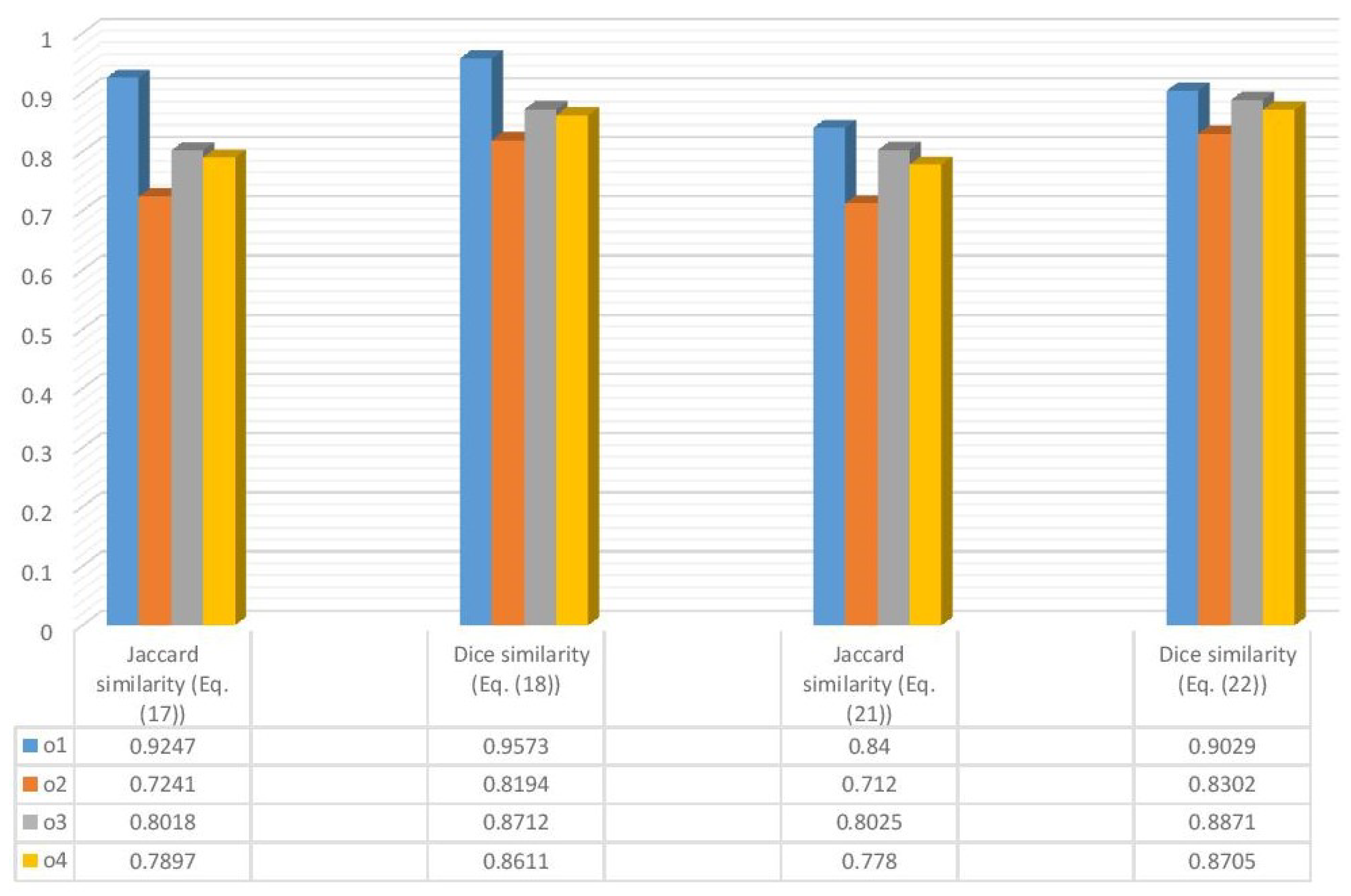
5.2. Sensitivity Analysis

In the present section, we describe our analysis of the influence of λ.

The main aim of sensitivity analysis is to analyze the impact of various values of the parameter λ on the decision outcomes. We use various values of λ in Step 5 of the method established in the present paper to address the considered problem. The ranking results are shown in Figure 2 and Figure 3 for Equations (32) and (33), respectively.

It can be noticed from

Table 2. Generalized Dice similarity measure of Equation (32) and ranking order.

$\mathit{\lambda }$	${\mathit{o}}_1$	${\mathit{o}}_2$	${\mathit{o}}_3$	${\mathit{o}}_4$	Ranking
0	$0.9061$	$1.2098$	$1.1761$	$1.1248$	$o_2>o_3>o_4>o_1$
$0.2$	$0.9221$	$0.9243$	$0.9421$	$0.8761$	$o_3>o_2>o_1>o_4$
$0.5$	$0.9573$	$0.8194$	$0.8712$	$0.8611$	$o_1>o_3>o_4>o_2$
$0.7$	$0.9947$	$0.8253$	$0.8875$	$0.915$	$o_1>o_4>o_3>o_2$
$0.9$	$1.0581$	$0.9433$	$0.9826$	$1.0493$	$o_1>o_4>o_3>o_2$
1	$1.1119$	$1.2149$	$1.1344$	$1.2223$	$o_4>o_2>o_3>o_1$

that ranking results are different for different values of λ in the developed approach, which means that our method is sensitive to the values of λ. According to Equation (32), when $\lambda =0$, the worst alternative, i.e., $o_2$ becomes the best one. Though the ranking results are different but from Table 2, we can see that for $\lambda =0.5,0.7$ and $0.9$, $o_1$ is the best alternative. Similarly, from

Table 3. Generalized Dice similarity measure of Equation (33) and ranking order.

$\mathit{\lambda }$	${\mathit{o}}_1$	${\mathit{o}}_2$	${\mathit{o}}_3$	${\mathit{o}}_4$	Ranking
0	$0.9227$	$0.9269$	$0.9969$	$0.9180$	$o_3>o_2>o_1>o_4$
$0.2$	$0.9401$	$0.8725$	$0.9355$	$0.8772$	$o_1>o_3>o_4>o_2$
$0.5$	$0.9029$	$0.8302$	$0.8871$	$0.8705$	$o_1>o_3>o_4>o_2$
$0.7$	$0.9911$	$0.8236$	$0.8720$	$0.8912$	$o_1>o_4>o_3>o_2$
$0.9$	$1.0147$	$0.8347$	$0.8663$	$0.9302$	$o_1>o_4>o_3>o_2$
1	$1.0276$	$0.8477$	$0.8659$	$0.9567$	$o_1>o_4>o_3>o_2$

, we can observe that $o_1$ is the most suitable alternative for all values of λ except 0. Therefore, according to different similarity measures and values of λ, ranking orders may also differ. Thus, the presented method can be assigned some measure and some value of λ to satisfy the requirement of DMs preferences and flexible decision-making.

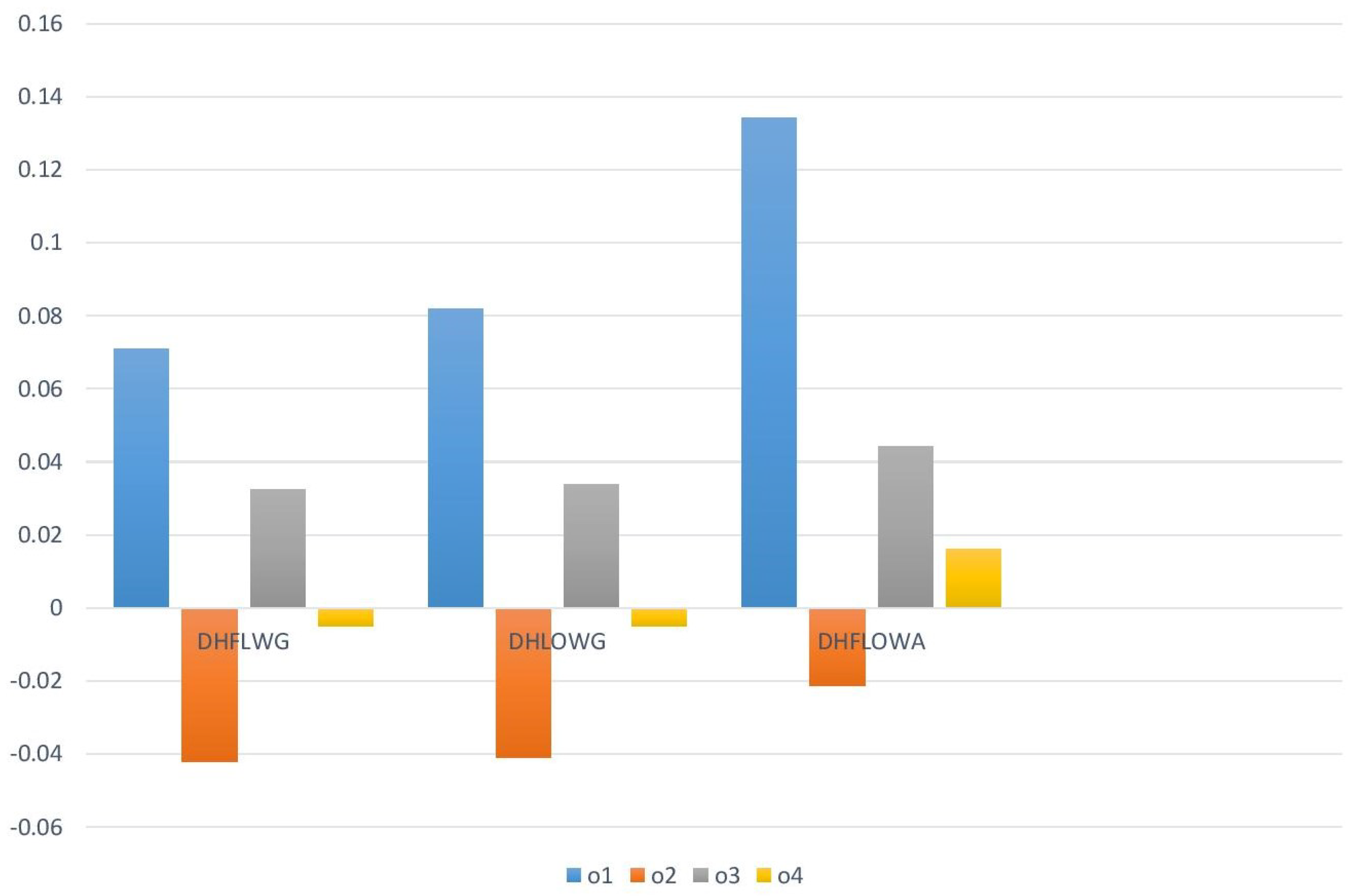
6. Comparative Analysis

In the present section, we conduct a comparative study with some existing approaches [17,18,56] in order to elaborate on the feasibility of the stated approach.

6.1. Solving by Dual Hesitant Fuzzy Linguistic Stochastic MCDM Method

Here, we solve the problem by the method based on regret theory developed by [18].

To save space, we only list the calculation results in the following. For a detailed study, please refer to Ref. [18].

Letting the regret aversion coefficient $\beta =0.3$, we obtain the regret value matrix $Q={\left(Q_{ji}\right)}_{4\times 4}$ and rejoice value matrix $\mathsf{\Gamma }={\left({\mathsf{\Gamma }}_{ji}\right)}_{4\times 4}$ of alternatives as

$$Q=\left(\begin{array}{cccc}0& -0.0114& 0& 0\\ -0.0112& 0& -0.0342& -0.0928\\ -0.0089& 0& 0& -0.0591\\ 0& -0.0138& -0.0610& 0\end{array}\right)$$

$$\mathsf{\Gamma }=\left(\begin{array}{cccc}0& 0.0436& 0.0575& 0.0849\\ 0.0151& 0& 0.0252& 0\\ 0.0173& 0.0544& 0& 0.0308\\ 0.0260& 0.0414& 0& 0\end{array}\right)$$

Using the weights obtained in Step 4 of the proposed approach, we obtain the comprehensive regret value $Q\left(o_j\right)$ and rejoice value $\mathsf{\Gamma }\left(o_j\right)$ as given below.

$$Q\left(o_1\right)=-0.0030,Q\left(o_2\right)=-0.0326,Q\left(o_3\right)=-0.0157,Q\left(o_4\right)=-0.0192;$$

$$\mathsf{\Gamma }\left(o_1\right)=0.0453,\mathsf{\Gamma }\left(o_2\right)=0.0103,\mathsf{\Gamma }\left(o_3\right)=0.0256,\mathsf{\Gamma }\left(o_4\right)=0.0175.$$

Based on the above values, we obtain the ranking assessment values as follows:

$$L\left(o_1\right)=0.0423,L\left(o_2\right)=-0.0223,L\left(o_3\right)=0.0099,L\left(o_4\right)=-0.0017.$$

Thus, the ranking is $o_1>o_3>o_4>o_2.$

From the above, it is clear that the results obtained by the stated approach are similar to the Qu et al. [18] algorithm, which guarantees that our method is effective. Likewise [18] approach, in the proposed method, DMs can select different values of λ according to their preferences. Moreover, DMs can also choose different similarity measures (18)/(32)/(22) or (33), to satisfy the real requirement. This makes our constructed method more flexible and general than existing models under the DHFL background. Moreover, Qu et al. [18] model is based on an irrational normalization process (as discussed in Section 2.2), and in the case of cost-type criteria may cause inaccuracies in the decision-making process. In such cases, it is more suitable to utilize the proposed approach as it is based on the revised complement operation of DHFLTs and is easy to understand. What is more, unlike some existing literature measures [35,37,57], the proposed similarity measures do not need to equalize the length of the corresponding DHFLEs, which makes the developed approach able to represent the original information about the situation.

6.2. Solving by Dual Hesitant Fuzzy Linguistic Aggregation-Based Method

In what follows, we employ some existing aggregation operators [17] to rank the alternatives. For instance, when we fuse the information given in Table 1 by utilizing the DHFLWG operator, then the aggregated results are obtained as

$$\begin{array}{cc}\hfill o_1=& \left\{〈s_{2.9045},\left\{0.3670,0.3917,0.3885,0.4146,0.3890,0.4152,0.4118,0.4395,0.4079,0.4354,0.4319,\right.\right.\hfill \\ \hfill & \left.0.4609,0.4072,0.4347,0.4311,0.4602,0.4317,0.4607,0.4569,0.4878,0.4527,0.4832,0.4793,0.5115\right\},\hfill \\ \hfill & \left.\left\{0.2333,0.2535,0.2635,0.2829,0.2968,0.3153,0.3245,0.3423\right\}〉\right\},\hfill \end{array}$$

$$\begin{array}{cc}\hfill o_2=& \left\{〈s_{2.9525},\left\{0.3311,0.3534,0.3469,0.3702,0.3680,0.3928,0.3856,0.4116,0.3506,0.3742,0.3673,\right.\right.\hfill \\ \hfill & \left.\left.0.3921,0.3898,0.4160,0.4083,0.4358\right\},\left\{0.4290,0.4571,0.4510,0.4781,0.4551,0.4819,0.4762,0.5020\right\}〉\right\},\hfill \end{array}$$

$$\begin{array}{cc}\hfill o_3=& \left\{〈s_{2.2898},\left\{0.5,0.5244\right\},\left\{0.3754,0.4006,0.4038,0.4279,0.4,0.4243,0.4273,0.4505,0.4039,0.4281,\right.\right.\hfill \\ \hfill & \left.\left.0.4311,0.4541,0.4275,0.4506,0.4535,0.4756\right\}〉\right\},\hfill \end{array}$$

$$\begin{array}{cc}\hfill o_4=& \left\{〈s_{2.2110},\left\{0.3476,0.3711,0.3973,0.4240,0.4166,0.4447,0.3858,0.4118,0.4409,0.4705,0.4624,0.4935\right\},\right.\hfill \\ \hfill & \left.\left\{0.3826,0.4368,0.4168,0.4680,0.4038,0.4561,0.4368,0.4862\right\}〉\right\}.\hfill \end{array}$$

Based on Equation (7), we obtain the score values of each alternative as follows:

$Sco\left(o_1\right)=0.0709,Sco\left(o_2\right)=-0.0420,Sco\left(o_3\right)=0.0325,Sco\left(o_4\right)=-0.0050.$

Analogously, we can apply the other operators to fuse the provided dual hesitant fuzzy linguistic information. The resultant values of the alternatives obtained through different operators and ranking orders are listed in

Table 4. Score values of alternatives and ranking order.

	${\mathit{o}}_1$	${\mathit{o}}_2$	${\mathit{o}}_3$	${\mathit{o}}_4$	Ranking
DHFLWG	$0.0709$	$-0.0420$	$0.0325$	$-0.0050$	$o_1>o_3>o_4>o_2$
DHFLOWG	$0.0819$	$-0.0411$	$0.0339$	$-0.0050$	$o_1>o_3>o_4>o_2$
DHFLOWA	$0.1342$	$-0.0214$	$0.0442$	$0.0162$	$o_1>o_3>o_4>o_2$

and shown in Figure 4.

From Table 4, it can be noticed that the most desirable alternative is $o_1$, and it coincides with the result of the stated approach.

Table 4 depicts that, as for the [17] approach, the aggregation-based method is also consistent with the presented model. By employing Spearman correlation [58] the coefficient values are given by $(1,1,1)$ with proposed vs. [17,18]. From the correlation values, it is clear that the developed method is highly consistent with existing ones. However, the gap between the score values of alternatives is larger than [18]. Thus, our constructed method has a stronger ability to discriminate between alternatives. Further, in practical situations, there will be certain risks and losses when we make decisions. The method established in the present paper can control these situations by altering the values of parameter λ. While the aggregation-based method [17] pays no attention to such a situation.

It is also necessary to point out that the [17] method is based on the assumption that the weight vector of criteria should be given in advance. However, our developed method can handle the dual-hesitant fuzzy linguistic decision-making problem with unknown weight information.

6.3. Solving by Dual Hesitant Fuzzy Similarity Measure-Based Method

To further check the validity and superiority of the propound approach, in the present section, we apply the dual hesitant fuzzy vector similarity measures approach [56] to address the aforementioned problem.

For this, we first transform the original information, which is provided in the form of DHFLTSs, into DHFSs by eliminating the linguistic component, as depicted in

Table 5. Dual hesitant fuzzy decision matrix D.

	${\mathit{c}}_1$	${\mathit{c}}_2$	${\mathit{c}}_3$	${\mathit{c}}_4$
$o_1$	$〈\left\{0.2,0.3\right\},\left\{0.3,0.5\right\}〉$	$〈\left\{0.4,0.5,0.6\right\},\left\{0.3,0.4\right\}〉$	$〈\left\{0.4,0.5\right\},\left\{0.2\right\}〉$	$〈\left\{0.6,0.8\right\},\left\{0.1,0.2\right\}〉$
$o_2$	$〈\left\{0.4,0.5\right\},\left\{0.4,0.5\right\}〉$	$〈\left\{0.2,0.3\right\},\left\{0.5\right\}〉$	$〈\left\{0.5,0.6\right\},\left\{0.3,0.4\right\}〉$	$〈\left\{0.3,0.4\right\},\left\{0.5,0.6\right\}〉$
$o_3$	$〈\left\{0.5\right\},\left\{0.4,0.5\right\}〉$	$〈\left\{0.5,0.6\right\},\left\{0.3,0.4\right\}〉$	$〈\left\{0.5\right\},\left\{0.4,0.5\right\}〉$	$〈\left\{0.5\right\},\left\{0.4,0.5\right\}〉$
$o_4$	$〈\left\{0.4,0.6\right\},\left\{0.4\right\}〉$	$〈\left\{0.3,0.5,0.6\right\},\left\{0.2,0.3\right\}〉$	$〈\left\{0.4\right\},\left\{0.5,0.6\right\}〉$	$〈\left\{0.3,0.4\right\},\left\{0.4,0.6\right\}〉$

.

In light of the dual hesitant fuzzy set’s score function, we acquire the following optimal solution:

$$p^{*}=\left\{〈\left\{0.4,0.6\right\},\left\{0.4\right\}〉,〈\left\{0.3,0.5,0.6\right\},\left\{0.2,0.3\right\}〉,〈\left\{0.4,0.5\right\},\left\{0.2\right\}〉,〈\left\{0.6,0.8\right\},\left\{0.1,0.2\right\}〉\right\}.$$

For better comparison, the same weights as determined in the schemed approach are utilized, i.e., $W={\left(0.2569,0.2611,0.2555,0.2265\right)}^T$.

Based on Guirao et al. [56] formulation, we calculate the weighted vector similarity measures amongst the alternative $o_i(i=1,2,3,4)$ and the optimal solution $p^{*}$ as follows:

Similarity measures obtained through the Jaccard measure: $J_w\left(o_1,p^{*}\right)=0.8852,$$J_w\left(o_2,p^{*}\right)=0.7405,$$J_w\left(o_3,p^{*}\right)=0.8242,$$J_w\left(o_4,p^{*}\right)=0.7801.$

Similarity measures obtained through the Dice measure: $D_w\left(o_1,p^{*}\right)=0.9348,$$D_w\left(o_2,p^{*}\right)=0.4173,$$D_w\left(o_3,p^{*}\right)=0.4449,$$D_w\left(o_4,p^{*}\right)=0.4276.$

Grounded on the generated similarity measures, we obtain the following ranking of evaluation alternatives: $o_1>o_3>o_4>o_2.$

The above ranking result shows that the alternative $o_1$ is again the optimal one, which is the same as identified by the developed approach. We can also see that the remainder of the choices are ranked in the same order. This demonstrates that the developed strategy achieves the same rankings as the existing ones [17,18,56]. This confirms that the suggested measures and techniques are legitimate and useful in the alternative selection process.

From Table 1, we can see that the information is provided in the form of DHFLTSs. We understand that existing similarity measures are incapable of undertaking such input. To make it possible, we reduced the provided data into a dual hesitant fuzzy context, as depicted in Table 5. As a result, we lost an essential component of the data, linguistic terms, which may lead to irrational decision results. Furthermore, Equations (11) and (12) of Ref. [56] do not describe the lengths of the membership and non-membership parts and will be nonsensical if these lengths are unequal. However, the correct form of these equations can be obtained from the proposed measures Equations (18) and (19) as follows:

$$\begin{array}{cc}\hfill {\mathcal{J}}_w^1\left(D_1,D_2\right)=& \frac{1}{2}{\displaystyle \sum _{i=1}^n}{w}_i\left(\frac{{\displaystyle \sum _{ı=1}^{\#g}}{\alpha }_{ı}\left({ɲ}_i\right)/\#g·{\displaystyle \sum _{ı=1}^{\#\overline{g}}}\overline{{\alpha }_{ı}}\left({ɲ}_i\right)/\#\overline{g}}{{\displaystyle \sum _{ı=1}^{\#g}}{\alpha }_{ı}^2\left({ɲ}_i\right)/\#g+{\displaystyle \sum _{ı=1}^{\#\overline{g}}}{\overline{{\alpha }_{ı}}}^2\left({ɲ}_i\right)/\#\overline{g}-{\displaystyle \sum _{ı=1}^{\#g}}{\alpha }_{ı}\left({ɲ}_i\right)/\#g·{\displaystyle \sum _{ı=1}^{\#\overline{g}}}\overline{{\alpha }_{ı}}\left({ɲ}_i\right)/\#\overline{g}}\right.\hfill \\ \hfill & +\left.\frac{{\displaystyle \sum _{ı=1}^{\#h}}{\beta }_{ı}\left({ɲ}_i\right)/\#h·{\displaystyle \sum _{ı=1}^{\#\overline{h}}}\overline{{\beta }_{ı}}\left({ɲ}_i\right)/\#\overline{h}}{{\displaystyle \sum _{ı=1}^{\#h}}{\beta }_{ı}^2\left({ɲ}_i\right)/\#h+{\displaystyle \sum _{ı=1}^{\#\overline{h}}}{\overline{{\beta }_{ı}}}^2\left({ɲ}_i\right)/\#\overline{h}-{\displaystyle \sum _{ı=1}^{\#h}}{\beta }_{ı}\left({ɲ}_i\right)/\#h·{\displaystyle \sum _{ı=1}^{\#\overline{h}}}\overline{{\beta }_{ı}}\left({ɲ}_i\right)/\#\overline{h}}\right),\hfill \end{array}$$

(42)

$${\mathcal{D}}_w^1\left(D_1,D_2\right)={\displaystyle \sum _{i=1}^n}{w}_i\left(\frac{{\displaystyle \sum _{ı=1}^{\#g}}{\alpha }_{ı}\left({ɲ}_i\right)/\#g·{\displaystyle \sum _{ı=1}^{\#\overline{g}}}\overline{{\alpha }_{ı}}\left({ɲ}_i\right)/\#\overline{g}}{{\displaystyle \sum _{ı=1}^{\#g}}{\alpha }_{ı}^2\left({ɲ}_i\right)/\#g+{\displaystyle \sum _{ı=1}^{\#\overline{g}}}{\overline{{\alpha }_{ı}}}^2\left({ɲ}_i\right)/\#\overline{g}}+\frac{{\displaystyle \sum _{ı=1}^{\#h}}{\beta }_{ı}\left({ɲ}_i\right)/\#h·{\displaystyle \sum _{ı=1}^{\#\overline{h}}}\overline{{\beta }_{ı}}\left({ɲ}_i\right)/\#\overline{h}}{{\displaystyle \sum _{ı=1}^{\#h}}{\beta }_{ı}^2\left({ɲ}_i\right)/\#h+{\displaystyle \sum _{ı=1}^{\#\overline{h}}}{\overline{{\beta }_{ı}}}^2\left({ɲ}_i\right)/\#\overline{h}}\right).$$

(43)

Thus, the similarity measures for DHFSs are particular cases of the similarity measures of DHFLTSs. Therefore, similarity measures propound in this article can be employed to determine not only the similarity measures for the problems with dual hesitant fuzzy linguistic data but also the similarity measures of the problems with dual hesitant fuzzy information, whereas the method in [56] is only suitable to calculate the similarity measures for DHFSs with equal lengths of the membership and non-membership parts.

Although the proposed measures have successfully generalized the structure of the existing measures, which demonstrates their breadth and innovations, the research work still has some limitations:

(i)

In some cases, DHFLTS can handle information. For instance, consider the DHFLE $d_1=\left\{{\upharpoonleft }_3,\left\{0.4,0.7\right\},\left\{0.3,0.4\right\}\right\}.$ Here ${\alpha }^{+}=0.7$ and ${\beta }^{+}=0.4$, clearly ${\alpha }^{+}+{\beta }^{+}>1$, therefore it does not satisfy the required criterion of DHFS, limiting the range of DHSs. Thus, the devised similarity measures of DHFLTS are unsuitable for solving problems with more uncertain information.

(ii)

In the created measures, we utilize the subscript of the linguistic terms directly in the process of operations, which may result in the loss of decision information.

7. Concluding Remarks and Suggestions

The DHFLTS, characterized by membership and non-membership functions, is an attractive generalization of the HFLTS. It was designed to facilitate complex scenarios based on linguistic knowledge. To enrich the theory of DHFLTS, the present paper first modified the definition of complement operation and then described the concept of information energy for DHFLTS. We also put forward the Jaccard and Dice similarity measures and their weighted forms. Later, some interesting properties of these similarity measures were also delineated. In addition, for DHFLTS, two types of generalized dice similarity measures and generalized weighted dice similarity measures were structured and analyzed. Based on the proposed information energy, a model was constructed to determine the fully unknown criteria weights objectively. Following that, we developed a similarity measure-based MCDM method with dual hesitant fuzzy linguistic contexts.The main merit of the stated method is that it is more general and flexible than the existing ones (with dual hesitant fuzzy linguistic environment). Because in this method, DMs can assign various values to the parameter λ to satisfy the real requirement. Finally, a practical case regarding money investment was addressed to demonstrate the practical use and effectiveness of the proposed measures and method. Sensitivity analysis and comparative study were also conducted, and it was observed that our method is highly consistent with existing literature methods, which confirmed the feasibility of the proposed method.

From the future research point of view, some interesting and noteworthy plans are pointed out as follows:

• In the literature, we can see that some scholars [51] have proposed an extension of HFLTS, namely DHFLTS. Even though its idea is a little different from the original DHFLTS [17]. Assigning the same name to different extensions creates confusion. Moreover, the notion [51] is complex and does not have good application potential. Therefore, there is a need to unify such types of extensions together.
• By introducing various dual hesitant fuzzy linguistic measures, we have opened new doors for building MCDM models under the DHFLTS context. Though in the current paper, we have constructed an MCDM model based on the proposed measures, but that is just a simple attempt, and we still need to construct some comprehensive similarity measure-based methods to model the complex scenarios with dual hesitant fuzzy linguistic information precisely.
• In the present paper, we limited ourselves to just defining information energy and did not shed light on the correlation coefficient, which is a well-used theoretical lens. After the introduction of information energy, now it is not very tough to study the correlation coefficient and weighted correlation coefficient for dual hesitant fuzzy linguistic background and apply them to the MCDM situation.
• To address some other related decision-making problems, such as pattern recognition, medical diagnosis, data mining, risk analysis, etc., via the proposed model is also an interesting research direction.

References

1. Zadeh, L.A. Fuzzy sets. Inf. Control. 1965, 8, 338–353. [Google Scholar] [CrossRef]
2. Malik, M.; Bashir, Z.; Rashid, T.; Ali, J. Probabilistic hesitant intuitionistic linguistic term sets in multi-attribute group decision making. Symmetry 2018, 10, 392. [Google Scholar] [CrossRef]
3. Bashir, Z.; Bashir, Y.; Rashid, T.; Ali, J.; Gao, W. A Novel Multi-Attribute Group Decision-Making Approach in the Framework of Proportional Dual Hesitant Fuzzy Sets. Appl. Sci. 2019, 9, 1232. [Google Scholar] [CrossRef]
4. Bashir, Z.; Ali, J.; Rashid, T. Consensus-based robust decision making methods under a novel study of probabilistic uncertain linguistic information and their application in Forex investment. Artif. Intell. Rev. 2020, 54, 2091–2132. [Google Scholar] [CrossRef]
5. Asiain, M.J.; Bustince, H.; Mesiar, R.; Kolesárová, A.; Takáč, Z. Negations with respect to admissible orders in the interval-valued fuzzy set theory. IEEE Trans. Fuzzy Syst. 2017, 26, 556–568. [Google Scholar] [CrossRef]
6. Ali, J.; Bashir, Z.; Rashid, T. WASPAS-based decision making methodology with unknown weight information under uncertain evaluations. Expert Syst. Appl. 2020, 15, 114143. [Google Scholar] [CrossRef]
7. Ali, J.; Bashir, Z.; Rashid, T. Weighted interval-valued dual-hesitant fuzzy sets and its application in teaching quality assessment. Soft Comput. 2020, 25, 3503–3530. [Google Scholar] [CrossRef]
8. Ali, J.; Garg, H. On spherical fuzzy distance measure and TAOV method for decision-making problems with incomplete weight information. Eng. Appl. Artif. Intell. 2023, 119, 105726. [Google Scholar] [CrossRef]
9. Herrera, F.; Herrera-Viedma, E. A model of consensus in group decision making under linguistic assessments. Fuzzy Sets Syst. 1996, 78, 73–87. [Google Scholar] [CrossRef]
10. Herrera, F.; Herrera-Viedma, E.; Verdegay, J.L. A rational consensus model in group decision making using linguistic assessments. Fuzzy Sets Syst. 1997, 88, 31–49. [Google Scholar] [CrossRef]
11. Xu, Z. Uncertain linguistic aggregation operators based approach to multiple attribute group decision making under uncertain linguistic environment. Inf. Sci. 2004, 168, 171–184. [Google Scholar] [CrossRef]
12. Xian, S.; Zhang, J.; Xue, W. Fuzzy linguistic induced generalized OWA operator and its application in fuzzy linguistic decision making. Int. J. Intell. Syst. 2016, 31, 749–762. [Google Scholar] [CrossRef]
13. Xian, S.; Sun, W.; Xu, S.; Gao, Y. Fuzzy linguistic induced OWA Minkowski distance operator and its application in group decision making. Pattern Anal. Appl. 2016, 19, 325–335. [Google Scholar] [CrossRef]
14. Rodriguez, R.M.; Martinez, L.; Herrera, F. Hesitant fuzzy linguistic term sets for decision making. IEEE Trans. Fuzzy Syst. 2011, 20, 109–119. [Google Scholar] [CrossRef]
15. Torra, V. Hesitant fuzzy sets. Int. J. Intell. Syst. 2010, 25, 529–539. [Google Scholar] [CrossRef]
16. Zadeh, L.A. The concept of a linguistic variable and its application to approximate reasoning—I. Inf. Sci. 1975, 8, 199–249. [Google Scholar] [CrossRef]
17. Yang, S.; Ju, Y. Dual hesitant fuzzy linguistic aggregation operators and their applications to multi-attribute decision making. J. Intell. Fuzzy Syst. 2014, 27, 1935–1947. [Google Scholar] [CrossRef]
18. Qu, G.; Xue, R.; Li, T.; Qu, W.; Xu, Z. A stochastic multi-attribute method for measuring sustainability performance of a supplier based on a triple bottom line approach in a dual hesitant fuzzy linguistic environment. Int. J. Environ. Res. Public Health 2020, 17, 2138. [Google Scholar] [CrossRef]
19. Zhang, R.; Xu, Z.; Gou, X. ELECTRE II method based on the cosine similarity to evaluate the performance of financial logistics enterprises under double hierarchy hesitant fuzzy linguistic environment. Fuzzy Optim. Decis. Mak. 2022, 1–27. [Google Scholar] [CrossRef]
20. Liu, D.; Chen, X.; Peng, D. Some cosine similarity measures and distance measures between q-rung orthopair fuzzy sets. Int. J. Intell. Syst. 2019, 34, 1572–1587. [Google Scholar] [CrossRef]
21. Wu, S.; Lin, J.; Zhang, Z. New distance measures of hesitant fuzzy linguistic term sets. Phys. Scr. 2020, 96, 015002. [Google Scholar] [CrossRef]
22. Wu, D.; Mendel, J.M. Similarity measures for closed general type-2 fuzzy sets: Overview, comparisons, and a geometric approach. IEEE Trans. Fuzzy Syst. 2018, 27, 515–526. [Google Scholar] [CrossRef]
23. Zhang, H.; Zhang, Z. Characteristic analysis of judgment debtors based on hesitant fuzzy linguistic clustering method. IEEE Access 2021, 9, 119147–119157. [Google Scholar] [CrossRef]
24. Egghe, L. Good properties of similarity measures and their complementarity. J. Am. Soc. Inf. Sci. Technol. 2010, 61, 2151–2160. [Google Scholar] [CrossRef]
25. Farhadinia, B.; Effati, S.; Chiclana, F. A family of similarity measures for q-rung orthopair fuzzy sets and their applications to multiple criteria decision making. Int. J. Intell. Syst. 2021, 36, 1535–1559. [Google Scholar] [CrossRef]
26. Ali, J.; Naeem, M. Cosine similarity measures between q-rung orthopair linguistic sets and their application to group decision making problems. Sci. Rep. 2022, 12, 14456. [Google Scholar] [CrossRef] [PubMed]
27. Ali, J.; Naeem, M. Distance and similarity measures for normal wiggly dual hesitant fuzzy sets and their application in medical diagnosis. Sci. Rep. 2022, 12, 13784. [Google Scholar] [CrossRef]
28. Singh, S.; Ganie, A.H. Applications of picture fuzzy similarity measures in pattern recognition, clustering, and MADM. Expert Syst. Appl. 2020, 168, 114264. [Google Scholar] [CrossRef]
29. Singh, A.; Kumar, S. A novel dice similarity measure for IFSs and its applications in pattern and face recognition. Expert Syst. Appl. 2020, 149, 113245. [Google Scholar] [CrossRef]
30. Ejegwa, P.A.; Agbetayo, J.M. Similarity-distance decision-making technique and its applications via intuitionistic fuzzy pairs. J. Comput. Cogn. Eng. 2022, 1–7. [Google Scholar] [CrossRef]
31. Beg, I.; Ashraf, S. Similarity measures for fuzzy sets. Appl. Comput. Math 2009, 8, 192–202. [Google Scholar]
32. Jun, Y. Vector similarity measures of hesitant fuzzy sets and their multiple attribute decision making. Econ. Comput. Econ. Cybern. Stud. Res. 2014, 48, 215–226. [Google Scholar]
33. Ye, J. The generalized Dice measures for multiple attribute decision making under simplified neutrosophic environments. J. Intell. Fuzzy Syst. 2016, 31, 663–671. [Google Scholar] [CrossRef]
34. Ejegwa, P.A. Distance and similarity measures for Pythagorean fuzzy sets. Granul. Comput. 2020, 5, 225–238. [Google Scholar] [CrossRef]
35. Song, Y.; Hu, J. Vector similarity measures of hesitant fuzzy linguistic term sets and their applications. PLoS ONE 2017, 12, e0189579. [Google Scholar] [CrossRef]
36. Wei, G.; Lin, R.; Lu, J.; Wu, J.; Wei, C. The generalized dice similarity measures for probabilistic uncertain linguistic MAGDM and its application to location planning of electric vehicle charging stations. Int. J. Fuzzy Syst. 2022, 24, 933–948. [Google Scholar] [CrossRef]
37. Zhang, Z.; Lin, J.; Miao, R.; Zhou, L. Novel distance and similarity measures on hesitant fuzzy linguistic term sets with application to pattern recognition. J. Intell. Fuzzy Syst. 2019, 37, 2981–2990. [Google Scholar] [CrossRef]
38. Verma, R. Generalized similarity measures under linguistic q-rung orthopair fuzzy environment with application to multiple attribute decision-making. Granul. Comput. 2022, 7, 253–275. [Google Scholar] [CrossRef]
39. Lee, H.M.; Chen, C.M.; Chen, J.M.; Jou, Y.L. An efficient fuzzy classifier with feature selection based on fuzzy entropy. IEEE Trans. Syst. Man, Cybern. Part B (Cybern.) 2001, 31, 426–432. [Google Scholar]
40. Pal, N.R.; Bustince, H.; Pagola, M.; Mukherjee, U.; Goswami, D.; Beliakov, G. Uncertainties with Atanassov’s intuitionistic fuzzy sets: Fuzziness and lack of knowledge. Inf. Sci. 2013, 228, 61–74. [Google Scholar] [CrossRef]
41. Wei, C.; Yan, F.; Rodríguez, R.M. Entropy measures for hesitant fuzzy sets and their application in multi-criteria decision-making. J. Intell. Fuzzy Syst. 2016, 31, 673–685. [Google Scholar] [CrossRef]
42. Xu, Z.; Xia, M. Hesitant fuzzy entropy and cross-entropy and their use in multiattribute decision-making. Int. J. Intell. Syst. 2012, 27, 799–822. [Google Scholar] [CrossRef]
43. Hung, C.C.; Chen, L.H. A fuzzy TOPSIS decision making model with entropy weight under intuitionistic fuzzy environment. In Proceedings of the International Multiconference of Engineers and Computer Scientists, IMECS, Hong Kong, China, 18–20 March 2009; Volume 1, pp. 13–16. [Google Scholar]
44. Zou, Z.H.; Yi, Y.; Sun, J.N. Entropy method for determination of weight of evaluating indicators in fuzzy synthetic evaluation for water quality assessment. J. Environ. Sci. 2006, 18, 1020–1023. [Google Scholar] [CrossRef] [PubMed]
45. Liu, M.; Ren, H. A new intuitionistic fuzzy entropy and application in multi-attribute decision making. Information 2014, 5, 587–601. [Google Scholar] [CrossRef]
46. Liu, P.; Shen, M.; Teng, F.; Zhu, B.; Rong, L.; Geng, Y. Double hierarchy hesitant fuzzy linguistic entropy-based TODIM approach using evidential theory. Inf. Sci. 2021, 547, 223–243. [Google Scholar] [CrossRef]
47. Aggarwal, M. Redefining fuzzy entropy with a general framework. Expert Syst. Appl. 2021, 164, 113671. [Google Scholar] [CrossRef]
48. Farhadinia, B.; Xu, Z. Novel hesitant fuzzy linguistic entropy and cross-entropy measures in multiple criteria decision making. Appl. Intell. 2018, 48, 3915–3927. [Google Scholar] [CrossRef]
49. Gou, X.; Xu, Z.; Liao, H. Hesitant fuzzy linguistic entropy and cross-entropy measures and alternative queuing method for multiple criteria decision making. Inf. Sci. 2017, 388, 225–246. [Google Scholar] [CrossRef]
50. Herrera, F.; Herrera-Viedma, E. Linguistic decision analysis: Steps for solving decision problems under linguistic information. Fuzzy Sets Syst. 2000, 115, 67–82. [Google Scholar] [CrossRef]
51. Zhang, R.; Li, Z.; Liao, H. Multiple-attribute decision-making method based on the correlation coefficient between dual hesitant fuzzy linguistic term sets. Knowl.-Based Syst. 2018, 159, 186–192. [Google Scholar] [CrossRef]
52. Dice, L.R. Measures of the amount of ecologic association between species. Ecology 1945, 26, 297–302. [Google Scholar] [CrossRef]
53. Jaccard, P. Distribution de la flore alpine dans le bassin des Dranses et dans quelques régions voisines. Bull. Soc. Vaudoise Sci. Nat. 1901, 37, 241–272. [Google Scholar]
54. Liao, H.; Xu, Z.; Zeng, X.J. Distance and similarity measures for hesitant fuzzy linguistic term sets and their application in multi-criteria decision making. Inf. Sci. 2014, 271, 125–142. [Google Scholar] [CrossRef]
55. Liao, H.; Xu, Z.; Zeng, X.J. Hesitant fuzzy linguistic VIKOR method and its application in qualitative multiple criteria decision making. IEEE Trans. Fuzzy Syst. 2014, 23, 1343–1355. [Google Scholar] [CrossRef]
56. Guirao, J.L.G.; Sarwar Sindhu, M.; Rashid, T.; Kashif, A. Multiple criteria decision-making based on vector similarity measures under the framework of dual hesitant fuzzy sets. Discret. Dyn. Nat. Soc. 2020, 2020, 1425487. [Google Scholar] [CrossRef]
57. Chai, J.; Xian, S.; Lu, S. Z-uncertain probabilistic linguistic variables and its application in emergency decision making for treatment of COVID-19 patients. Int. J. Intell. Syst. 2021, 36, 362–402. [Google Scholar] [CrossRef]
58. Spearman, C. The proof and measurement of association between two things. Am. J. Psychol. 1904, 15, 72–101. [Google Scholar] [CrossRef]
Figure 1. Ranking order of alternatives using different similarity measures.
Symmetry 15 00471 g001
Figure 2. Impact of different values of λ on alternatives using Equation (32).
Symmetry 15 00471 g002
Figure 3. Impact of different values of λ on alternatives using Equation (33).
Symmetry 15 00471 g003
Figure 4. Aggregation operators based ranking of alternatives.
Symmetry 15 00471 g004