Abstract
In this work, an improved symmetric integral barrier function-based tracking control is addressed for a robotic manipulator in the presence of position error performance requirements and unknown uncertain terms. First of all, we construct an improved symmetric time-variant integral barrier function to solve the robotic system’s constrained requirements. The novel barrier function is constructed by developing an integral upper limit function that can be used in conjunction with existing performance envelope functions. Then, the equivalent conversion error is taken as the upper limit of the integral function to achieve the specified steady-state as well as transient behaviors of the system. Additionally, a disturbance observer based on the velocity tracking error is introduced to compensate for unknown uncertain terms. In the end, a numeral simulation study on a robot with two degrees is performed to indicate that the present scheme is feasible in handling the performance constraint and uncertain terms.
1. Introduction
Nowadays, human daily lives require robots more and more [1,2,3,4,5,6]. Low-precision trajectory tracking or path tracing control possesses a high possibility of resulting in the failure of control tasks or even leading to safety accidents. For robots, it is inevitable that they require high-precision control when replacing humans to complete specific tasks, especially when interacting with humans. Tracking control, as the core link of robot control systems, has been presented with many advanced control methods [7,8,9,10,11,12]. Among these effective methods, an inter-neural computing method is used in path following control of mobile robots to track the reference path produced by tracked targets [13]. Aimed at path-following control of robotic manipulators under disturbance, unknown dynamics, and kinematics, an approach in the framework of the sliding mode observer is presented to improve the control accuracy [14]. The Jacobian matrix pseudo-inverse technique of only using the input and output signal is applied to controlling the uncertain robotic manipulators [15]. In [16], a task-space path-following issue of a robot under unknown kinematics and dynamics is studied to make the system state trend to the equilibrium point exponentially. This method ensures the exponential convergence of the robot system for the first time. Aimed at the tracking control of robot manipulators subject to disturbances as well as input torque limits, a model predictive control scheme is presented to guarantee input-to-output stability of the robotic system [17]. Tracking control, as a necessary and fundamental issue for robots in the automotive, aviation, medical, and other fields, is receiving more and more attention from scholars. Nevertheless, the issue of the performance requirements in robot tracking control is not considered in most of the above-mentioned articles.
For the issue of performance requirements, a performance envelope function is usually constructed to ensure the error trends to zero within the specified envelope, thereby ensuring steady-state and transient behaviors of the system. There are two main strategies used in prescribed performance control. In the first strategy, the performance envelope function and error with requirements of performance limitations are used together to transform into an unconstrained space. In the second strategy, envelope functions and the barrier Lyapunov function (BLF) are applied together to adjust the system control performance. A tangential error transformation function, for instance, is used to prescribe the tracking performance of the mobile robot [18]. In [19,20], the tracking error with a performance constraint requirement is transformed into an unconstrained error in logarithmic form, and then the constrained error always remains within the specified performance range by ensuring the boundedness of the conversion error. In [21], to clarify the explicit convergence time of errors, an improved performance envelope function is constructed to ensure the control effects of Autonomous Underwater Vehicles. For the second strategy, a performance envelope function and BLF, for example, are integrated to maintain the transient indicator of hydraulic systems [22]. Additionally, the combination of the performance envelope function and BLF is also used to guarantee the preset transient behavior of uncertain Euler–Lagrange systems [23]. Since performance control strategies were first proposed, they have been widely used in ensuring the transient and steady-state indicators of systems. This performance-constrained idea is worthy of use for reference in this article.
With the growth of the need for robot control systems in various industries, the control performance indicators of the robot are being taken seriously, which is directly indicated by transient behavior and steady-state error. The conventional adaptive tracking control scheme guarantees that the system errors trend to the bounded set [24,25,26,27,28,29]. However, determining how to design tracking control to ensure the performance requirements of the robotic system is still a challenge. The error in performance requirements of the robotic system is transformed via the performance envelope function to improve the transient response speed as well as the final stable error [30]. In [31], by constructing two smooth monotonic functions to complete the error transformation, a control scheme of a logarithmic BLF embedding the transformed error is presented to guarantee the performance requirements of the robot manipulators. In [32], a time-variant logarithmic BLF combining a performance envelope function is used to directly ensure the transient behavior and steady-state behavior of the robot. Therefore, to facilitate the design of the control scheme, we hope to eliminate complex error transformation, while designing simpler BLF functions to achieve the performance constraints directly.
In this work, we try to design a performance-guaranteed tracking controller based on improved symmetric time-variant BLF for the robotic system. The contribution points are described as follows:
- (1)
- Enlightened by the form of the existing logarithmic and integral BLF, we propose an improved time-variant integral BLF, which is constructed by mapping out an integral upper limit function that can be used in conjunction with existing performance envelope functions. The advantage of the proposed integral barrier function is that it is easy to combine with existing performance envelope functions to achieve constraints on time-varying transient and steady-state performance [33,34].
- (2)
- The proposed control strategy only needs to normalize the error with performance-constrained requirements using the performance envelope function and then directly utilize the proposed BLF to complete performance constraint control without complex error transformation [35]. The controller design is simple and easy to implement.
- (3)
- Unlike existing integral BLFs [33,34,36,37,38], the presented BLF can deal with time-variant and symmetric constraint problems of nonlinear systems. Under the presented scheme based on this BLF, the performance requirements of the robot are always met, while the exponentially asymptotic stability of the system is obtained.
The remaining work in this article is planned as follows: Section 2 illuminates the problem statement and preparation. Section 3 tries to design a performance-guaranteed tracking control for the robot based on the improved BLF, and the system stability is discussed. The numerical simulation study of a robot with two degrees is completed in Section 4. The contents of the study are summarized in Section 5.
2. Problem Statement and Preparation
2.1. Robot’s Dynamics
A robotic system with n degrees of freedom is modeled as [39,40,41]
where denotes the position of the robotic manipulators, represents the product of a Jacobian matrix and external forces, stands for the gravitational matrix and Coriolis-centripetal torque, respectively, denotes the symmetric positive inertia matrix, the control input of the manipulators is represented by , and the overall uncertainty is represented by .
Remark 1.
The model of the robotic manipulators is derived from [39,40,41]. The joints of robot manipulators are all revolute joints. Because the position (joint angle) and velocity (joint angular velocity) are known, the angular acceleration can logically be obtained. In order to ensure the smooth derivation of the controller, we will perform coordinate transformation to convert system (1) into a multi-input and multi-output system.
2.2. System Transformation and Control Objective
For the convenience of controller design, we let and . Then, the multi-input and multi-output system can be described as
The Control Objective works to combine the improved integral barrier function proposed for the first time in this article with the existing performance envelope function to design a performance-guaranteed trajectory-tracking controller for robotic manipulators. Under the designed control, it can ensure that the position vector (joint angle) can smoothly track the desired target , and the position error is always limited within the performance envelope function , with and being the positive constant, that is, .
Remark 2.
The performance envelope function used in this article is referred to from [42]. Enlightened by the idea of existing performance constraints, the performance-guaranteed problem can be converted to the boundary constraint problem of error . In order to use the performance envelope function in conjunction with the BLF proposed in this article, we normalize the position errors as , . According to the definition of , we can determine that the inequalities and are equivalent.
Assumption 1.
The overall uncertainty is supposed to be bounded, differentiable, and slowly varying, that is, , such that and , .
Remark 3.
We know that the system uncertainty is related to the joint angle (position) and joint angular velocity (velocity) of the robot. The joint angles and velocities of the system exist and are bounded, so we make reasonable assumptions about the boundedness of uncertainty. In addition, the state of the system is continuous and differentiable, and it will not jump under normal circumstances; therefore, it is reasonable to assume the existence of uncertainty derivatives. The assumption that the derivative of uncertainty is a slowly time-varying signal is for a class of robot systems that are less affected by external interference and the robotic arm end has flexibility. This assumption has certain limitations, but it has certain significance in theoretical research.
Remark 4.
The assumption of slowly varying lumped uncertainties has appeared in many articles, such that the derivative of the unknown terms in the tracking control of ships is assumed to be zero, namely, in [43]. The external disturbances are often regarded as slowly varying signals with regard to the inertial frame. In the motion control of the robots, the lumped disturbance usually consists of both external disturbance and model uncertainty. The assumption that the derivative of the lumped disturbance is zero is often considered when no further information is provided [44,45]. The assumption for the robot systems that are less affected by external interference and the robotic arm end has flexibility is meaningful, such as writing robots and B-ultrasound detection robots.
2.3. Improved Barrier Function
Definition 1.
The definition of the improved integral barrier function over the open set is given as
In view of the definition of , it can be seen that is radially unbounded as approaches 1, continuous, positive, and differentiable in the set .
Theorem 1.
In the set , the improved barrier function defined in (3) is of the following property.
Proof.
(I) Firstly, we prove that holds. An auxiliary function is constructed as
Taking the derivative with respect to normalization error, yields
We can obtain that as and as over the open set . In addition, is true always when . As a result, holds all the time over the open set .
(II) The inequality will be proven next. Firstly, the second auxiliary function is defined.
Solving the derivation with respect to normalization error yields
From the derivative of , we can obtain that as and as over the open set . Further, in terms of the definition of , we know that as . Thus, the inequality holds over the open set . The proof of Theorem 1 ends here.
3. Performance-Guaranteed Control Design
With the help of the backstepping method, the controller based on the improved integral BLF is designed in this section. To begin with, consider the following BLF.
In the set , according to the definition of normalization error , differentiating yields
Differentiating , we can obtain
And
where .
Taking (12) into (10) becomes
By means of the backstepping method, the desired value of is chosen as
And
where
and with being positive constants.
Substituting (15) into (13) yields
The inequality holds at all times, thus, in the open set , (18) can be rewritten as
Taking the derivation of yields
Inspired by [20], the observer based on the derivative of is introduced as
where , is the setting parameter of the observer, and signifies the observer’s state. signifies the estimation of with being the estimating error.
To obtain the control law , the second Lyapunov function is constructed as
Taking the derivation of (22), we obtain
The controller is given as
where
and is the positive definite matrix.
Next, we will prove the tracking control system is stable.
Theorem 2.
For the robotic system (2), considering the uncertain terms and performance-constrained requirement under Assumption 1 with the controllers (14) and (24) and observer (21) and if the initial position errors meet , then (I) the position vector can be successful in tracking the preset path , (II) the position error vector remains within the performance envelope function, that is , and (III) the system’s errors are exponentially asymptotically stable.
Proof.
Considering (20), (23) becomes
In view of Assumption 1, substituting the derivation of and (24) into (26) yields
where denotes the n-order identity matrix.
When assigning values to parameters and , it is necessary to ensure that the following inequalities are true
With the aid of Theorem 1, (27) can be altered as
where
Next, we use mathematical methods to elucidate Theorem 2. Finding the solution of the differential Equation (29) yields
Invoking (9) and (22), we obtain
Combining (31) and the definition of , we have
where
we know that is bounded.
Solving the inequality (33), we have and .
By further analysis, it is clear that the inequalities and hold when , and the inequalities and are true when . In conclusion, we have and .
With the aid of Theorem 1 and in view of (31), we have
According to (35) and the definition of the normalization error , we obtain . To summarize, the system’s error signals can trend to zero exponentially and asymptotically, while the position error signal always satisfies performance constraint conditions. At this point, the complete proof process of Theorem 2 has been provided.
Remark 5.
To the best of the author’s knowledge, the existing prescribed performance control, such as [20,46], can only guarantee that the performance-constrained error of the system is located within the pre-set boundary, that is, the steady-state error satisfies . However, with the aid of the given Theorem 1 in this article, the presented prescribed performance control method based on the improved integral BLF not only ensures that the performance-constrained error always falls within the envelope function but also that the performance-constrained error can trend to zero asymptotically.
Remark 6.
The performance index of an automatic control system can be divided into transient and steady-state performances. In order to ensure the convergence rate of the system, finite-time stability [47] and fixed-time stability [48] theories are proposed. Unfortunately, finite time and fixed time control only ensure that the tracking error tends to zero within a finite or fixed time, without excessive requirements for overshoot and steady-state error. However, the proposed barrier function can be directly combined with the appointed-time performance envelope function to ensure that the tracking error trends to zero within the user-defined time, while also constraining the maximum overshoot and limiting the steady-state error to a certain region. In future work, the proposed method will be combined with the appointed time performance function to ensure faster convergence of the system.
4. Simulation
In this section, a robot with two degrees is utilized for the numerical simulations to confirm the effectiveness of the improved BLF-based performance-constrained tracking control scheme. The architecture of the closed-loop system is depicted in Figure 1, where the P-function denotes the performance envelope function and BLF represents the barrier Lyapunov function.
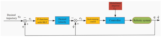
Figure 1.
Architecture of the closed-loop system.
The position vector is chosen as
Considering previous studies [39,41], the robotic system’s relevant matrixes are given below:
where
Please refer to [39,41] for the physical meanings of the above parameters and variables.
The initial position and velocity set in the simulation are given as
The reference path is set as
The system’s unknown term is given as
In order to guarantee the position performance-constrained conditions , hold, the performance envelope function’s parameters are set as , , and , and the parameters of the controller and observer are chosen as , , , and .
Remark 7.
The larger the gain of position tracking error , the faster the convergence of the tracking error, but it will lead to a larger control input, which easily leads to actuator saturation. The larger the control gain of the speed tracking error , the smaller the steady-state error, but when it increases to a certain extent, the simulation experiment will fail. The impact of the parameter on control performance is minimal, as long as it is a very small positive number. When the parameter of the observer , the observed value is the smallest. If the parameter selection of the performance envelope function is not appropriate, such as being too small, the required control input will be very large. If the limit of the actuator is reached, it is easy to cause failure of the control task.
The simulation results of the performance-constrained tracking control for the robot with two degrees are depicted in Figure 2, Figure 3, Figure 4, Figure 5, Figure 6 and Figure 7. Figure 2 and Figure 3 show the effects of the robot’s arms and tracking the reference path, as well as the ability to constrain the steady-state and transient behaviors of the position error. The effect of the velocity tracking the target value is given in Figure 4. Figure 5 depicts the observed effect of the observer. The control inputs of each robotic arm are given in Figure 6. Figure 7 describes the overall effect of two robotic arms tracking the circular path.
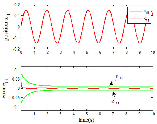
Figure 2.
Tracking effect of .
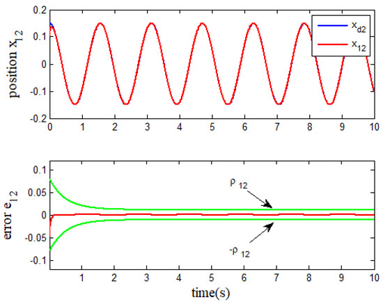
Figure 3.
Tracking effect of .
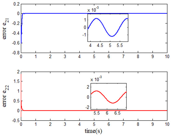
Figure 4.
Velocity error .
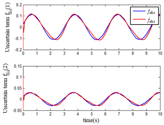
Figure 5.
Uncertain terms.
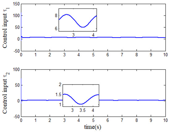
Figure 6.
Control inputs.
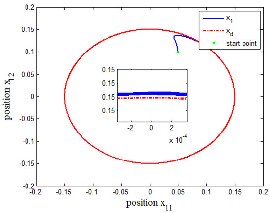
Figure 7.
Phase portrait of and .
Further analysis of Figure 2 and Figure 3 shows that the performance envelope functions and are not violated at all times, and the controller based on the improved integral BLF can provide a good tracking performance. In Figure 4, the initial velocity error is significant, but it quickly trends to a small area near zero. We know that the system uncertainty is related to the joint angle (position) and joint angular velocity (velocity) of the robotic system. In addition, the state of the system is continuous and differentiable, and it will not jump under normal circumstances. From Figure 5, we can see the uncertain terms are relatively smooth and the estimation error is large in the initial time. However, the estimated value quickly tracked the target value with acceptable accuracy in this simulation environment. From Figure 6, we can see that only at the initial moment does the robotic arm need to provide significant torque to enable the robot to track the reference path. In Figure 7, the comprehensive phase portrait of and tracking the reference circular path shows that the presented improved BLF is successful in designing the tracking control scheme for the robotic system.
Remark 8.
In the simulation, we have verified the feasibility of the proposed method. We only conducted one simulation case, and due to the numerous achievements of using existing barrier functions for performance constraints, we did not perform repetitive work to complete comparative simulation experiments with them. In addition, the designed observer has slightly poor estimation performance for unknown terms and will be improved in future works. Moreover, the control input is large in the initial time and can easily cause saturation of the robot’s executing mechanism. When the developed control strategy requires more control input than the maximum value provided by robotic actuators, the constraint control will be unsuccessful. Therefore, in order to prevent actuator saturation, we need to carefully set the parameters of the constraint boundary function. The performance function used in this article is from [42]. Since the method proposed in this article does not require complex error transformations, we will improve the performance envelope function in future research directions to make it easier to combine with the proposed barrier function. Finally, we would like to apply our proposed method to the semi-physical simulation platform of robot manipulators for verification.
5. Conclusions and Future Research
This study addresses an improved symmetric time-variant integral BLF-based performance-guaranteed tracking control problem of a robot with n-degrees. Utilizing the structural characteristics of the presented BLF combined with normalization errors directly handles the performance constraints of the systems without complex error transformations. The structure of the BLF is built by designing an integral upper limit function that can be directly combined with existing performance envelope functions and has universality. We indicate that the robotic system’s exponential asymptotic stability can be obtained by the proposed Theorem 1 and Lyapunov analysis, and the steady-state and transient behaviors of the system position error are located within the pre-set performance envelope at all times under the designed controller. In the end, the main results of this work are verified through numerical simulation.
In future work, we will combine the proposed barrier function with the specified time performance envelope function and adaptive control techniques to handle uncertain systems with the requirements of precise convergence time. In addition, from the simulation results, it can be seen that the initial control input is greatly increased, which leads to actuator saturation and even control task failure. Therefore, we will incorporate actuator saturation control technology into the proposed control algorithm. Finally, the proposed integral function is only for symmetric performance constraints, and we will change the symmetric barrier function to an asymmetric form.
Author Contributions
Conceptualization, T.Z. and P.Y.; methodology, T.Z.; software, T.Z.; validation, T.Z. and P.Y.; formal analysis, P.Y.; investigation, T.Z.; resources, T.Z.; data curation, T.Z.; writing—original draft preparation, T.Z.; writing—review and editing, T.Z.; visualization T.Z.; supervision, T.Z.; project administration, T.Z.; funding acquisition, P.Y. All authors have read and agreed to the published version of the manuscript.
Funding
This work is supported in part by the Start-up Fee for Scientific Research of High-level Talents in 2022 under Grant No. WGKQ2022006, in part by the Scientific Research Projects of Universities in Anhui Province under Grant No. 2022AH051674, and in part by the School Level Quality Engineering Project under Grant No. wxxy2022097.
Data Availability Statement
All data utilized to support the findings of this paper are contained in the paper.
Acknowledgments
This research was funded by the Start-up Fee for Scientific Research of High-level Talents in 2022 under Grant No. WGKQ2022006, the Scientific Research Projects of Universities in Anhui Province under Grant No. 2022AH051674, and in part by the School Level Quality Engineering Project under Grant No. wxxy2022097. We would like to thank everyone who has contributed to this article. We also would like to thank the anonymous reviewers and editors for their helpful suggestions and comments.
Conflicts of Interest
The authors declare no conflict of interest.
References
- Huang, P.; Zhang, F.; Cai, J.; Wang, D.; Meng, Z.; Guo, J. Dexterous tethered space robot: Design, measurement, control, and experiment. IEEE Trans. Aerosp. Electron. Syst. 2017, 53, 1452–1468. [Google Scholar] [CrossRef]
- He, W.; Li, Z.; Chen, C.L.P. A survey of human-centered intelligent robots: Issues and challenges. IEEE/CAA J. Autom. Sin. 2017, 4, 602–609. [Google Scholar] [CrossRef]
- He, W.; Ge, W.; Li, Y.; Liu, Y.-J.; Yang, C.; Sun, C. Model identification and control design for a humanoid robot. IEEE Trans. Syst. Man Cybern. Syst. 2017, 47, 45–57. [Google Scholar] [CrossRef]
- Wang, H.; Wang, C.; Chen, W.; Liang, X.; Liu, Y. Three-dimensional dynamics for cable-driven soft manipulator. IEEE/ASME Trans. Mechatron. 2017, 22, 18–28. [Google Scholar] [CrossRef]
- Li, Z.; Huang, B.; Ajoudani, A.; Yang, C.; Su, C.-Y.; Bicchi, A. Asymmetric bimanual control of dual-arm exoskeletons for human-cooperative manipulations. IEEE Trans. Robot 2018, 34, 264–271. [Google Scholar] [CrossRef]
- Gao, Z.; Shi, Q.; Fukuda, T.; Li, C.; Huang, Q. An overview of biomimetic robots with animal behaviors. Neurocomputing 2019, 332, 339–350. [Google Scholar] [CrossRef]
- Castaño, M.L.; Tan, X. Backstepping-Based Tracking Control of Underactuated Aquatic Robots. IEEE Trans. Control Syst. Technol. 2023, 31, 1179–1195. [Google Scholar] [CrossRef]
- Xie, C.; Fan, Y.; Qiu, J. Event-based tracking control for nonholonomic mobile robots. Nonlinear Anal. Hybrid Syst. 2020, 38, 100945. [Google Scholar] [CrossRef]
- Juang, L.-H.; Zhang, J.-S. Visual Tracking Control of Humanoid Robot. IEEE Access 2019, 7, 29213–29222. [Google Scholar] [CrossRef]
- Ahmadi, S.; Fateh, M. On the Taylor series asymptotic tracking control of robots. Robotica 2019, 37, 405–427. [Google Scholar] [CrossRef]
- Wang, H.; Chen, G.; Zhang, W. A method for vehicle speed tracking by controlling driving robot. Trans. Inst. Meas. Control 2020, 42, 1521–1536. [Google Scholar] [CrossRef]
- Khan, M.U.; Li, S.; Wang, Q.; Shao, Z. Formation Control and Tracking for Co-operative Robots with Non-holonomic Constraints. J. Intell. Robot. Syst. 2016, 82, 163–174. [Google Scholar] [CrossRef]
- Tsai, F.-S.; Hsu, S.-Y.; Shih, M.-H. Adaptive Tracking Control for Robots with an Interneural Computing Scheme. IEEE Trans. Neural Netw. Learn. Syst. 2018, 29, 832–844. [Google Scholar] [CrossRef] [PubMed]
- Xiao, B.; Yin, S.; Kaynak, O. Tracking Control of Robotic Manipulators with Uncertain Kinematics and Dynamics. IEEE Trans. Ind. Electron. 2016, 63, 6439–6449. [Google Scholar] [CrossRef]
- Chen, D.; Zhang, Y.; Li, S. Tracking Control of Robot Manipulators with Unknown Models: A Jacobian-Matrix-Adaption Method. IEEE Trans. Ind. Inform. 2018, 14, 3044–3053. [Google Scholar] [CrossRef]
- Xiao, B.; Yin, S. Exponential Tracking Control of Robotic Manipulators with Uncertain Dynamics and Kinematics. IEEE Trans. Ind. Inform. 2019, 15, 689–698. [Google Scholar] [CrossRef]
- Dai, L.; Yu, Y.; Zhai, D.-H.; Huang, T.; Xia, Y. Robust Model Predictive Tracking Control for Robot Manipulators with Disturbances. IEEE Trans. Ind. Electron. 2021, 68, 4288–4297. [Google Scholar] [CrossRef]
- Fu, D.; Huang, J.; Yin, H. Controlling an uncertain mobile robot with prescribed performance. Nonlinear Dyn. 2021, 106, 2347–2362. [Google Scholar] [CrossRef]
- Xia, H.; Chen, J.; Lan, F.; Liu, Z. Motion Control of Autonomous Vehicles with Guaranteed Prescribed Performance. Int. J. Control Autom. Syst. 2023, 18, 1510–1517. [Google Scholar] [CrossRef]
- Zheng, Z.; Feroskhan, M. Path Following of a Surface Vessel with Prescribed Performance in the Presence of Input Saturation and External Disturbances. IEEE ASME Trans. Mechatron. 2017, 22, 2564–2575. [Google Scholar] [CrossRef]
- Sun, Y.; Zhang, Y.; Qin, H.; Ouyang, L.; Jing, R. Predefined-time prescribed performance control for AUV with improved performance function and error transformation. Ocean Eng. 2023, 281, 114817. [Google Scholar] [CrossRef]
- Xu, Z.; Deng, W.; Shen, H.; Yao, J. Extended-State-Observer-Based Adaptive Prescribed Performance Control for Hydraulic Systems with Full-State Constraints. IEEE ASME Trans. Mechatron. 2022, 27, 5615–5625. [Google Scholar] [CrossRef]
- Hu, Y.; Yan, H.; Zhang, Y.; Zhang, H.; Chang, Y. Event-Triggered Prescribed Performance Fuzzy Fault-Tolerant Control for Unknown Euler-Lagrange Systems with Any Bounded Initial Values. IEEE Trans. Fuzzy Syst. 2023, 31, 2065–2075. [Google Scholar] [CrossRef]
- Azhdari, M.; Binazadeh, T. Uniformly ultimately bounded tracking control of sandwich systems with nonsymmetric sandwiched dead-zone nonlinearity and input saturation constraint. J. Vib. Control 2022, 28, 1109–1125. [Google Scholar] [CrossRef]
- Zhang, H.; Wei, X.; Karimi, H.R.; Han, J. Anti-disturbance control based on disturbance observer for nonlinear systems with bounded disturbances. J. Franklin Inst. 2018, 355, 4916–4930. [Google Scholar] [CrossRef]
- Wang, W.; Tong, S. Adaptive Fuzzy Bounded Control for Consensus of Multiple Strict-Feedback Nonlinear Systems. IEEE Trans. Cybern. 2018, 48, 522–531. [Google Scholar] [CrossRef]
- Yin, H.; Chen, Y.-H.; Yu, D.; Lü, H.; Shangguang, W. Adaptive robust control for a soft robotic snake: A smooth-zone approach. Appl. Math. Model. 2020, 80, 454–471. [Google Scholar] [CrossRef]
- Zhen, S.; Ma, M.; Liu, X.; Chen, F.; Zhao, H.; Chen, Y.-H. Model-based robust control design and experimental validation of SCARA robot system with uncertainty. Appl. J. Vib. Control 2023, 29, 91–104. [Google Scholar] [CrossRef]
- Dong, Y.; He, W.; Kong, L.; Hua, X. Impedance Control for Coordinated Robots by State and Output Feedback. IEEE Trans. Syst. Man Cybern. Syst. 2021, 51, 5056–5066. [Google Scholar] [CrossRef]
- Zhang, Y.; Fang, L.; Song, T.; Zhang, M. Adaptive non-singular fast terminal sliding mode based on prescribed performance for robot manipulators. Asian J. Control 2023, 25, 3253–3268. [Google Scholar] [CrossRef]
- Lyu, W.; Zhai, D.-H.; Xiong, Y.; Xia, Y. Predefined performance adaptive control of robotic manipulators with dynamic uncertainties and input saturation constraints. J. Franklin Inst. 2021, 358, 7142–7169. [Google Scholar] [CrossRef]
- Huang, H.; He, W.; Li, J.; Xu, B.; Yang, C.; Zhang, W. Disturbance Observer-Based Fault-Tolerant Control for Robotic Systems with Guaranteed Prescribed Performance. IEEE Trans. Cybern. 2022, 52, 772–783. [Google Scholar] [CrossRef] [PubMed]
- Zhang, J. Integral Barrier Lyapunov Functions-based Neural Control for Strict-feedback Nonlinear Systems with Multi-constraint. Int. J. Control Autom. Syst. 2018, 16, 2002–2010. [Google Scholar] [CrossRef]
- Zhao, B.; Feng, Z.; Guo, J. Integral barrier Lyapunov functions-based integrated guidance and control design for strap-down missile with field-of-view constraint. Trans. Inst. Meas. Control 2021, 43, 1464–1477. [Google Scholar] [CrossRef]
- Dong, C.; He, S.; Dai, S.-L. Performance-Guaranteed Tracking Control of an Autonomous Surface Vessel with Parametric Uncertainties and Time-Varying Disturbances. IEEE Access 2019, 7, 101905–101914. [Google Scholar] [CrossRef]
- Li, D.-J.; Li, J.; Li, S. Adaptive control of nonlinear systems with full state constraints using Integral Barrier Lyapunov Functionals. Neurocomputing 2016, 186, 90–96. [Google Scholar] [CrossRef]
- Liu, L.; Liu, Y.-J.; Chen, A.; Tong, S.; Chen, C.L. Integral Barrier Lyapunov function-based adaptive control for switched nonlinear systems. Sci. China Inf. Sci. 2020, 63, 132203. [Google Scholar] [CrossRef]
- Tang, Z.-L.; Ge, S.S.; Tee, K.P.; He, W. Robust Adaptive Neural Tracking Control for a Class of Perturbed Uncertain Nonlinear Systems with State Constraints. IEEE Trans. Syst. Man Cybern. Syst. 2016, 46, 1618–1629. [Google Scholar] [CrossRef]
- Liu, Y.-J.; Lu, S.; Tong, S. Neural Network Controller Design for an Uncertain Robot with Time-Varying Output Constraint. IEEE Trans. Syst. Man Cybern. Syst. 2017, 47, 2060–2068. [Google Scholar] [CrossRef]
- Liang, X.; Wang, H.; Zhang, Y. Adaptive nonsingular terminal sliding mode control for rehabilitation robots. Comput. Electr. Eng. 2022, 99, 107718. [Google Scholar] [CrossRef]
- He, W.; Chen, Y.; Yin, Z. Adaptive Neural Network Control of an Uncertain Robot with Full-State Constraints. IEEE Trans. Cybern. 2016, 46, 620–629. [Google Scholar] [CrossRef] [PubMed]
- Bechlioulis, C.P.; Rovithakis, G.A. Robust Adaptive Control of Feedback Linearizable MIMO Nonlinear Systems with Prescribed Performance. IEEE Trans. Autom. Control 2008, 53, 2090–2099. [Google Scholar] [CrossRef]
- Godhavn, J.-M.; Fossen, T.I.; Berge, S.P. Non-linear and adaptive backstepping designs for tracking control of ships. Int. J. Adapt. Control Signal Process. 1998, 12, 649–670. [Google Scholar] [CrossRef]
- Veil, C.; Muller, D.; Sawodny, O. Nonlinear disturbance observers for robotic continuum manipulators. Mechatronics 2021, 78, 102518. [Google Scholar] [CrossRef]
- Muller, D.; Veil, C.; Seidel, M.; Sawodny, O. Disturbance Observer Based Control for Quasi Continuum Manipulators. IFAC-PapersOnLine 2020, 53, 9808–9813. [Google Scholar] [CrossRef]
- Chen, F.; Dimarogonas, D.V. Leader-Follower Formation Control with Prescribed Performance Guarantees. IEEE Trans. Control Netw. Syst 2021, 8, 450–461. [Google Scholar] [CrossRef]
- Wang, F.; Gao, H.; Wang, K.; Zhou, C.; Zong, Q.; Hua, C. Disturbance Observer-Based Finite-Time Control Design for a Quadrotor UAV with External Disturbance. IEEE Trans. Aerosp. Electron. Sys. 2021, 57, 834–847. [Google Scholar] [CrossRef]
- Liu, K.; Wang, R. Antisaturation Adaptive Fixed-Time Sliding Mode Controller Design to Achieve Faster Convergence Rate and Its Application. IEEE Trans. Circuit Syst. II Express Briefs 2022, 69, 3555–3559. [Google Scholar] [CrossRef]
Disclaimer/Publisher’s Note: The statements, opinions and data contained in all publications are solely those of the individual author(s) and contributor(s) and not of MDPI and/or the editor(s). MDPI and/or the editor(s) disclaim responsibility for any injury to people or property resulting from any ideas, methods, instructions or products referred to in the content. |
© 2023 by the authors. Licensee MDPI, Basel, Switzerland. This article is an open access article distributed under the terms and conditions of the Creative Commons Attribution (CC BY) license (https://creativecommons.org/licenses/by/4.0/).