Short-Term Photovoltaic Power Forecasting Based on a Novel Autoformer Model

Abstract

Deep learning techniques excel at capturing and understanding the symmetry inherent in data patterns and non-linear properties of photovoltaic (PV) power, therefore they achieve excellent performance on short-term PV power forecasting. In order to produce more precise and detailed forecasting results, this research suggests a novel Autoformer model with De-Stationary Attention and Multi-Scale framework (ADAMS) for short-term PV power forecasting. In this approach, the multi-scale framework is applied to the Autoformer model to capture the inter-dependencies and specificities of each scale. Furthermore, the de-stationary attention is incorporated into an auto-correlation mechanism for more efficient non-stationary information extraction. Based on the operational data from a 1058.4 kW PV facility in Central Australia, the ADAMS model and the other six baseline models are compared with 5 min and 1 h temporal resolution PV power data predictions. The results show in terms of four performance measurements, the proposed method can handle the task of projecting short-term PV output more effectively than other methods. Taking the result of predicting the PV energy in the next 24 h based on the 1 h resolution data as an example, MSE is 0.280, MAE is 0.302, RMSE is 0.529, and adjusted R-squared is 0.824.

1. Introduction

The growing need for clean energy around the world may be partially met by photovoltaic (PV) power, a renewable, safe, and adaptable distributed energy supply [1]. Over the past few decades, PV power has drawn more attention [2]; its integration has had substantial positive effects on the economy and the environment. Due to its erratic and intermittent nature, significant PV penetration, however, also poses a number of new difficulties for the operation of current grid systems [3]. These difficulties include intermittent power generation, high installation costs, and the PV power supply’s vulnerability to weather conditions [4]. Forecasting PV electricity is an effective way to deal with these difficulties. For large-scale PV penetration in the primary power grid, precise forecasting of PV energy generation is acknowledged as a requirement [5]. The approaches of forecasting PV power can be categorized into three groups depending on the forecasting time horizon: long-term PV power forecasting (LTPVF), middle-term PV power forecasting (MTPVF), and short-term PV power forecasting (STPVF). Short-term forecasting is the process of predicting the amount of PV power that will be produced over the next hour, several hours, day, or even seven days. Forecasting for medium-term PV electricity is performed over periods of time longer than a week to a month. The long-term forecasts of PV power generation range from one month to one year.

Many studies have been conducted recently that go in-depth on the subject of short-term photovoltaic power forecasting (STPVF). The traditional statistical method, e.g., the Autoregressive Integrated Moving Average (ARIMA) was previously employed as the initial STPVF attempt. Support vector machine (SVM), Gaussian process regression (GPR) and extreme learning machine (ELM) are three conventional machine learning (ML) models that are used frequently in STPVF. However, in the STPVF challenge with complex and lengthy data, these techniques perform poorly. The dependable forecasting performance needed for the construction of reliable PV energy systems cannot be attained by standard methodologies for PV energy prediction. Deep learning (DL) techniques based on neural networks are significantly more favored than typical statistical approaches and machine learning techniques for understanding the long-term patterns of PV power data. Recently, both STPVF situations have used a variety of deep learning neural networks, including recurrent neural network (RNN), gated recurrent units (GRU), long short-term memory (LSTM), convolutional neural network (CNN) and transformer-based models. Deep learning approaches have been used to make some progress, although these techniques still have major drawbacks. As an illustration, consider single-step forecasting, sophisticated computing, and significant memory costs.

Furthermore, it was commonly acknowledged in earlier studies to use a decomposition technique or stationarization to pre-process time series for nonstationary and nonlinear signals. This can make the raw time series less complex and non-stationary, which will increase prediction accuracy and provide deep models a more stable data distribution. Decomposition and stationarization are typically used to pre-process historical data before projecting future series for forecasting activities. However, this pre-processing is constrained by the simple decomposition impact of historical series and ignores the series’ long-term hierarchical interaction with its underlying patterns. Wu et al. suggested Autoformer as an alternative to transformers for long-term time series prediction based on the concept of decomposition [6]. The Autoformer model is enabled to split the information about long-term trends of anticipated hidden series gradually by embedding deconstruction blocks as the internal operators. The inherent non-stationarity of real-world time series, however, also serves as useful guidance for identifying temporal connections for forecasting. For predicting real-world burst events, the stationarized series that lacks inherent non-stationarity may be less useful.

In response to the above-mentioned drawbacks, we propose a novel Autoformer model with de-stationary attention and multi-scale framework (ADAMS) for the research of STPVF. The forecast modeling of PV power data is performed for capturing and understanding the symmetry inherent and non-stationarity in data patterns by the ADAMS model and employing it in order to predict future PV power data. On the Yulara datasets, where the PV power data is taken from DKASC, which is located at the Desert Knowledge Precinct in Central Australia, the performance of the proposed model is validated. Large random variations and non-stationary data patterns are present in this data. Therefore, it is essential to be able to recover the fluctuation curves while assessing the performance of models. ADAMS performs satisfactorily in the experiment while forecasting fluctuation curves. Additionally, the suggested ADAMS has reduced compute complexity and memory cost to 0(L logL), and it can perform several steps of predicting. The primary innovations and novelties in this paper are as follows:

• An improved ADAMS model is proposed for STPVF. The extra multi-scale framework and de-stationary attention is added to the Autoformer model. According to the results, the ADAMS is contributing to extract features more deeply and handle complicated, non-stationary data, which lowers forecasting error.
• Some additional methods are used as the baselines to test the efficacy of the ADAMS that is proposed. Autoformer, Informer, Transformer, LSTM, GRU, and RNN are all used in this paper. They are utilized for short-term PV power forecast with prediction lengths of 4 to 24. The MSE, MAE, RMSE, and adjusted R-squared $\left(R_a^2\right)$ were employed as evaluation measures for accuracy.
• More tests with a temporal resolution of one hour were conducted to further demonstrate the usefulness of the proposed ADAMS. According to expectations, the suggested ADAMS model achieves the best performance across all experimental forecasting models when compared to earlier projects, giving strong evidence that the suggested model works.

The remainder of this research is organized as follows: the second section gives a detailed summary of previous work relevant to STPVF. The third section introduces thoroughly the suggested ADAMS neural network. Next, the fourth section illustrates the experimental preparation and framework. The fifth section contains the STPVF experiment using ADAMS and the analysis of the result. Finally, the sixth section sums up this study.

2. Related Work

Time series statistical analysis known as ARIMA is commonly employed in forecasting. Numerous academics have assessed the model in various forecasting applications. While the forecasting accuracy increased as the forecasting horizon was expanded, ARIMA has performed poorly in long-term time series. Because the long-term data has a lot of high-dimension hidden features, there are not enough parameters in ARIMA, which prevents it from fitting these long-term data.

Machine learning techniques have recently been suggested for forecasting PV power. Traditional techniques of machine learning, such as SVM, are frequently suggested for predicting PV power. In a study they released in 2020, Pan et al. shown that using SVM for the very short-term prediction is feasible and using ant colony optimization to determine the best parameters of this model [7]. For the purpose of anticipating hourly PV power generation, Zhou et al. used the ELM to model the input features, a genetic algorithm to optimize the relevant parameters of their forecasting model [8]. They also adopted a customized similar day analysis based on five meteorological components.

Despite the widespread use of ML techniques, there are still a number of significant drawbacks, including the following: (1) they heavily depend on the quality of the feature engineering used; (2) they are unable to deal with complex feature scenarios with high irregularity; and (3) they exhibit unstable predictive power, making them inappropriate as a component for the reliable decision making required for any power system. They are unsuitable as a part of the trustworthy decision-making required for any power system since they have unstable forecasting ability, strongly depend on the level of the feature engineering employed, and are unable to handle complicated feature situations with high irregularity. Consequently, to provide more accurate predictions, ML algorithms are frequently integrated with other methods.

Recurrent networks are effective in simulating dependencies in sequential data, as shown in recent DL literature. Because of its ability to extract hidden information during graph processing using the convolution principle, CNN has received a lot of attention in the field of computer vision (CV). A growing number of studies have been published on hybrid CNN models for PV power forecasting in order to adapt to time-series forecasting applications. A CNN-BiGRU hybrid technique was suggested in one study by Zhang et al. to anticipate PV power for a PV power facility in Korea range [9]. Zang et al. used a hybrid method based on CNN to precisely predict how much energy a short-term photovoltaic system would produce [10]. The training time series must be brief due to the convolution calculation’s high computing complexity, and a lack of data could result in a major overfitting issue. In natural language processing, RNN and its unique variant, LSTM, which is built with a memory cell architecture to record essential information, have been frequently proposed. The LSTM and RNN techniques have been suggested in prior studies for STPVF. For instance, Gao et al. proposed a day-ahead power output time-series forecasting methods based on LSTM, in which ideal weather type and non-ideal weather types have been separately discussed [11].

Thanks to its capability to manage long-term interdependence without disappearing gradient, LSTM has been widely used. However, location information and long-term correlations are frequently present in energy time series, therefore the LSTM is unable to acquire a major amount of input properties that can have a considerable impact on prediction performance. Additionally, because of the restricted computer memory, both LSTM and RNN approaches can only predict one timestep forward, which takes more time if the aim is to provide the prediction of multiple timesteps ahead. This difficulty is caused by the enormous memory occupation. However, error accumulation, the fatal flaw in single-step forecasting, significantly enhanced the unreliability of forecasting multiple timesteps in advance.

In 2017, the Transformer model, which is well-known for its self-attention mechanism, was suggested and is currently being employed in the field of NLP [12]. The self-attention mechanisms and the enhanced later version, which have replaced the conventional memory block in LSTM and the initial attention mechanism, have produced more accuracy in longer language comprehension. Some academics think it might increase the capacity for prediction. However, it cannot be directly implemented to time series forecasting because of the high computation time, large memory utilization, and abrupt decline in forecasting rate. Many academics have worked hard and provided numerous solutions to these problems. The sparse decomposition of the attention matrix is considered in Ref. [13]. The logsparse Transformer is proposed in Ref. [14], which adds a convolutional self-attention mechanism. Longformer, a linear expansion of the attention mechanism with series length, is introduced in Ref. [15]. The complication of the entire self-attention in time and space is reduced by a novel self-attention mechanism in Ref. [16]. An improved version of Transformer called Informer, which has been tried on four sizable data sets, is established in Ref. [17]. It offers an alternative answer to the time series prediction issue. However, rather than concentrating on a section of the time series, all of these approaches with better self-attention only do so for an individual historical period. Due to the exceedingly small attention horizon, the single self-attention worked quite badly when the training data had significant variations.

Wu et al. used an enhanced self-attention method called auto-correlation in a work they released in 2021 in which they took advantage of a decomposition architecture [6]. The NBEATS model and high accuracy on the power price dataset were achieved by Oreshkin and his colleagues, who also introduced the canonical decomposition architecture [18]. The input dimension does, however, have a limit on the original NBEATS. With the use of an auto-correlation mechanism and a decomposition block, Autoformer built on the concept of temporal decomposition [19]. Additionally, Autoformer forecasts very long future data in a single computing step, which takes much less time. In light of the fact that the Autoformer model obtains high accuracy on numerous datasets but has not been used for the STPVF job, this research suggests an ADAMS model that will eventually produce a favorable forecasting accuracy for the STPVF.

3. ADAMS Network Architecture

The goal of PV power forecasting is to estimate future length L_pred from historical length L_seq. For multi-step forecasting, a new ADAMS is suggested in this paper. The complexity and non-stationarity of data and the calculation efficiency are the two key difficulties in PV power forecasting, as mentioned previously. To solve these problems:

• In addition to replacing the conventional self-attention mechanism, the auto-correlation mechanism serves to identify temporally dependent trends in large historical data sets.
• The de-stationary module is incorporated to the auto-correlation mechanism to acquire hidden characteristics from the non-stationary time series data. In this way, the model can not only retain the important information of the original sequence, but also eliminate the non-stationarity of the original data.
• A projected time series is refined iteratively at many scales with shared weights using the multi-scale framework, introducing changes to the architecture and a normalization method that was especially created to produce considerable speed increases with little additional computational effort.

3.1. Decomposition Architecture

To break down complex time patterns into more predictable parts, a deep decomposition architecture [6] with embedded sequence decomposition is introduced.

3.1.1. Series Decomposition Block

One of the most crucial techniques for time series forecasting is decomposition, which can divide the series into trend-cyclical and seasonal components, to learn about complicated temporal information in the context of long-term forecasting. These two sections each depict the series’ long-term development and seasonality. However, since the future is simply uncertain, direct decomposition is not feasible for next series. We introduce a series decomposing block as an internal operation of model to address this conundrum. This block can gradually recover the long-term stable trend from projected intermediary hidden factors. To put it more specifically, we modify the moving average to eliminate cyclical variations and emphasize long-term trends. The procedure is as follows for length $L$ input series $X\in {ℝ}^{L\times d}$:

$$\begin{array}{c}{X}_t=\mathrm{AvgPool}\left(\mathrm{Padding}\left(X\right)\right)\\ X_s=X-X_t,\end{array}$$

(1)

where, respectively, $X_s, X_t\in R^L\times d$ indicate the seasonal and trend-cyclical components that were extracted. To maintain the same series length, we use the $\mathrm{AvgPool}\left(\cdot \right)$ moving average with the padding procedure. To summarize the aforementioned equations, which is a model inner block, we utilize:

$$X_s, X_t=\mathrm{SeriesDecomp}\left(X\right).$$

(2)

3.1.2. Model Inputs

The past $L_{seq}$ time steps $X_{en}$ serve as the encoder part’s inputs. The seasonal part is denoted as $X_{des}$. $X_{det}$ stand for the trend-cyclical part. In order to be refined, $X_{des}$ and $X_{det}$ are both present in the input of the ADAMS model decoder. Each initialization has two components: a placeholder with length $O$ filled with scalars, and a component deconstructed from the second half $X_{en}$, with length $L_{seq}/2$ to supply late information. $X_{en}$ is the input of the encoder. It is expressed as follows:

$$\begin{array}{c}{X}_{ens},X_{ent}=\mathrm{SeriesDecomp}\left(X_{en\left(\frac{L_{\mathrm{seq}}}{2} : L_{\mathrm{seq}}\right)}\right)\\ X_{des}=\mathrm{Concat}\left(X_{ens},X_0\right)\\ X_{det}=\mathrm{Concat}\left(X_{ent},X_{\mathrm{mean}}\right),\end{array}$$

(3)

where $X_{ens}, X_{ent}$, respectively, represent the cyclical and seasonal elements of $X_{en}$, and $X_0, X_{mean}$, respectively, stand for the blank spaces filled with $0$ and the average of $X_{en}$.

3.1.3. Encoder

The encoder concentrates on the seasonal component modeling. Past seasonal data from the encoder’s output will be used as cross information to help the decoder improve forecast outcomes. Let us say there are $N$ encoder layers. The summary equations for the $l$-th encoder layer are $X_{en}^l=\mathrm{Encoder}(X_{en}^{l-1})$. Details are shown as follows:

$$\begin{array}{c}{S}_{en}^{l,1},\_=\mathrm{SeriesDecomp}\left(\mathrm{Auto}-\mathrm{Correlation}\left(X_{en}^{l-1}\right)+X_{en}^{l-1}\right)\\ S_{en}^{l,2},\_=\mathrm{SeriesDecomp}\left(\mathrm{FeedForward}\left(S_{en}^{l,1}\right)+S_{en}^{l,1}\right),\end{array}$$

(4)

where “_” denotes the portion of the trend that was deleted. The output of the $l$-th encoder layer is indicated by $X_{en}^l=S_{en}^{l,2},l\in \left\{1,\dots ,L\right\}$. $X_{en}^l$ is the embedded $X_{en}$. The seasonal component is represented as $S_{en}^{l,i},i\in \left\{1, 2\right\}$ after the $i$-th series decomposition block in the $l$-th layer, respectively.

3.1.4. Decoder

The accumulating architecture for trend-cyclical elements and the layered auto-correlation technique for seasonal elements are both included in the decoder. The internal auto-correlation and encoder-decoder auto-correlation found in each decoder layer allow for the improvement of prediction and use of historical seasonal data, respectively. It should be noted that the architecture collects the prospective trend from the intermediary hidden variables throughout the decoder, enabling the model to gradually improve the trend forecasting and remove disturbance information for the discovery of addictions based on the period in the auto-correlation. Assume there are $M$ layers in the decoder. The equations of the $l$-th decoder layer can be condensed as $X_{de}^l=\mathrm{Decoder}\left(X_{de}^{l-1}+X_{en}^N\right)$ using the potential variable $X_{en}^N$ from the encoder. It is possible to formalize the decoder as follows:

$$\begin{array}{c}\left.S_{de}^{l,1},T_{de}^{l,1}=\mathrm{SeriesDecomp}(\mathrm{Auto}-\mathrm{Correlation}\left(X_{de}^{l-1}\right)+X_{de}^{l-1}\right)\\ \left.S_{de}^{l,2},T_{de}^{l,2}=\mathrm{SeriesDecomp}(\mathrm{Auto}-\mathrm{Correlation}\left(S_{de}^{l,1},X_{en}^N\right)+S_{de}^{l,1}\right)\\ \left.S_{de}^{l,3},T_{de}^{l3}=\mathrm{SeriesDecomp}(\mathrm{FeedForward}\left(S_{de}^{l,2}\right)+S_{de}^{l,2}\right)\\ T_{de}^l=T_{de}^{l-1}+W_{l,1}*T_{de}^{l,1}+W_{l,2}*T_{de}^{l,2}+W_{l,3}*T_{de}^{l,3},\end{array}$$

(5)

where the output of the $l$-th decoder layer is indicated by $X_{de}^l=S_{de}^{l,3},l\in \left\{1,\dots ,L\right\}$. The $i$-th sequence decomposition in the $l$-th layer is represented by $S_{de}^{l,i},T_{de}^{l,i},i\in \left\{1,2,3\right\}$, which stand for seasonal factors and periodic factors, respectively. The projector for the $i$-th extracted trend $T_{de}^{l,i},i\in \left\{1,2,3\right\}$ is represented by $W_{l,3}$.

3.2. Auto-Correlation Mechanism

For the purpose of realizing series-wise connections and making better use of the information in the sequence, the auto-correlation technique [6] is added to substitute the attention method of point-to-point connections. In this module, based on the theory of random process, the self-attention mechanism of point-wise connection is discarded, and the auto-correlation technique of series-wise connection is realized, which has complexity and breaks the bottleneck of information utilization.

3.2.1. Period-Based Dependencies

The similar phasing points across eras is seen to actually produce identical sub-processes. For a real separate-time series $\left\{X_t\right\}$, we can use the following equations to derive the autocorrelation, which can be expressed as:

$$R_{XX}\left(\tau \right)=\underset{L\to +\infty }{lim}\frac{1}{L}{\displaystyle \sum }_{t=1}^L{X}_t{X}_{t-\tau }.$$

(6)

The resemblance between $\left\{X_t\right\}$ and lag $\tau$ series $\left\{X_{t-\tau }\right\}$ is reflected by $R_{XX}\left(\tau \right)$. We utilize the autocorrelation $R_{XX}\left(\tau \right)$ as the unnormalized confidence of the anticipated period length. After the calculation process, the largest feasible range of $k$ period lengths ${\tau }_1,\dots ,{\tau }_k$ are selected. The aforementioned estimated periods are used to construct the period-based dependencies, which can then be weighted using the relevant autocorrelation.

3.2.2. Time Delay Aggregation

The sub-series are connected between estimated periods by the period-based dependencies. In order to roll the series based on a chosen time lag of ${\tau }_1,\dots ,{\tau }_k$, we therefore provide the time delay aggregation block. In contrast to the point-wise dot-product aggregation in the self-attention mechanism, this process can line up same sub-series that are in the similar phasing point of predicted periods. The sub-series is then combined using softmax normalized confidences.

We receive query $Q$, key $K$, and value $V$ for the alone head scenario and series $X$ with length-$L$ after the projection process. It can thus easily take the role of self-attention. The process of auto-correlation is presented as below:

$$\begin{array}{l}{\tau }_1,{\tau }_2,\dots ,{\tau }_k=\underset{\tau \in \left\{1,2,\dots ,L\right\}}{\arg \mathrm{Top}K}\left(R_{Q,K\left({\tau }_k\right)}\right)\\ {\widehat{R}}_{Q,K\left({\tau }_1\right)},\dots ,{\widehat{R}}_{Q,K\left({\tau }_k\right)}=\mathrm{Softmax}\left(R_{Q,K\left({\tau }_1\right)},\dots ,R_{Q,K\left({\tau }_k\right)}\right)\\ \mathrm{Auto}-\mathrm{Correlation} \left(Q,K,V\right)={\displaystyle \sum _{i=1}^k}\mathrm{Roll}\left(V,{\tau }_i\right){\widehat{R}}_{Q,K}\left({\tau }_i\right),\end{array}$$

(7)

where, $c$ is a hyper-parameter. Let $⎣k=c\times \log L⎦$, and $\arg TopK\left(\cdot \right)$ is to obtain the arguments of the $TopK$ autocorrelations. The series $Q$ and $K$ have an autocorrelation called $R_{Q,K}$. The process to $X$ with time lag is represented by $Roll\left(X,\mathsf{\tau }\right)$. It causes components that have been moved past the first position to be reintroduced at the last position. $K$, $V$ are from the encoder $X_{en}^N$ and will be scaled to length-$O$, and $Q$ is from the previous block of the decoder for the encoder-decoder auto-correlation.

For the multi-head version adopted in this paper, with $d_{model}$ channels, $h$ heads, and the $i$-th head’s query, key, and value denoted as $Q_i, K_i, V_i$ individually. The multi-head auto-correlation are calculated as:

$$\begin{array}{c}\mathrm{Multi}-\mathrm{H}\mathrm{e}\mathrm{a}\mathrm{d}\left(Q,K,V\right)=W_{\mathrm{output}.}*\mathrm{Concat}\left({\mathrm{h}\mathrm{e}\mathrm{a}\mathrm{d}}_1,\dots ,{\mathrm{h}\mathrm{e}\mathrm{a}\mathrm{d}}_h\right)\\ {\mathrm{where} \mathrm{head}}_i=\mathrm{Auto}-\mathrm{Correlation}\left(Q_i,K_i,V_i\right).\end{array}$$

(8)

3.2.3. Efficient Computation

Period-based dependencies are intrinsically sparse and point to sub-processes that are in the similia phasing place as the parent period. In this case, we choose the longest delays in order to avoid choosing the opposite phases. Equations (7) and (8) have an $O\left(L logL\right)$ complexity due to the fact that we aggregate series with length $L$. Based on the Wiener-Khinchin theorem, when the time series $\left\{X_t\right\}$ are given, $R_{XX}\left(\tau \right)$ can be determined using Fast Fourier-Transforms for the autocorrelation computation (Equation (6)).

$$\begin{array}{c}{S}_{XX}\left(f\right)=F\left(X_t\right)\tilde{\mathcal{F}}\left(X_t\right)={{\displaystyle \int }}_{-\infty }^{+\infty }{X}_t{e}^{-j*2\pi tf}dt\overline{{{\displaystyle \int }}_{?\infty }^{+\infty }{X}_t{e}^{-j2\pi tf}dt}\\ R_{XX}\left(\tau \right)={\mathcal{F}}^{-1}\left(S_{XX}\left(f\right)\right)={{\displaystyle \int }}_{-\infty }^{+\infty }{S}_{XX}\left(f\right)e^{i2\pi f\tau }df,\\ \end{array}$$

(9)

where ${\mathcal{F}}^{-1}$ is the FFT’s inverse and $\tau \in \left\{1,\dots ,L\right\}$, $\mathcal{F}$ stands for the FFT. $S_{XX}\left(f\right)$ is in the frequency domain, and “∗” denotes the conjugate operation. It should be noted that the FFT may calculate the series autocorrelation of all lags in $\left\{1,\dots ,L\right\}$ at once. Auto-correlation achieves $O\left(L logL\right)$ complexity as a result.

3.3. Multi-Scale Framework

For accurate time series prediction, it is necessary to introduce structural prior considering multi-scale information. Autoformer introduced some emphasis on scale-awareness by mandating separate computational routes for the trend and seasonal components of the input time series. However, this structural prior only concentrated on two scales: low-frequency and high-frequency components. A multi-scale framework [20] with a cross-scale normalizing mechanism was created in order to detect the timing dependent patterns in long history data and to substitute for the conventional self-attention method in light of their significance to forecasting. We present an original iterative scale-refinement paradigm that is easily adaptable to various transformer-based time series forecasting architectures. At the same time, we apply cross-scale normalization to the transformer’s outputs to reduce distribution shifts between scales and windows.

We repeatedly apply the same neural module at various temporal scales given an input time-series $X^{\left(L\right)}$. The initial look-back window $X^{\left(L\right)}$ is fed into the encoder at $i$-th step $\left(0\le i\le m\right)$ after being scaled down by a factor of $s_i\equiv s^{m-i}$ using an average pooling operation. On the other hand, a linear interpolation is used to upsample the input to the decoder $X_{i-1}^{\mathrm{out}}$ by a factor of $s$. The array of $0s$ is used to initialize the variable $X_i^{\mathrm{dec}}$. The model carries out the following tasks:

$$\begin{array}{c}{x}_{t,i}=\frac{1}{s_i}{\displaystyle \sum _{\tau +1}^{\tau +s_i}}{x}_{\tau },\tau =t\times s_i\\ X_i^{\left(L\right)}=\left\{x_{t,i}|\frac{t_0}{s_i}\le t\le \frac{t_0+l_L}{s_i}\right\}\\ X_i^{\left(H\right)}=\left\{x_{t,i}|\frac{t_0+l_L+1}{s_i}\le t\le \frac{t_0+l_L+l_H}{s_i}\right\},\end{array}$$

(10)

where $X_i^{\left(L\right)}$ and $X_i^{\left(H\right)}$ are the look-back and horizon windows at the $i$-th step at time $t$, respectively. We may define $X_i^{\mathrm{enc}}$ and $X_i^{\mathrm{dec}}$ as the inputs to the normalization if we assume that ${x^{\prime }}_{t,i-1}$ is the output of the forecasting module at step $i-1$ and time $t$:

$$\begin{array}{c}{X}_i^{\mathrm{enc}}=X_i^{\left(L\right)}\\ {x^{″}}_{t,i}={x^{\prime }}_{⎣t/s⎦,i-1}+\left({x^{\prime }}_{⎣t/s⎦,i-1}-{x^{\prime }}_{⎣t/s⎦,i-1}\right)\times \frac{t-⎣t/s⎦}{s}\\ X_i^{\mathrm{dec}}=\left\{{x^{″}}_{t,i}\right|\frac{t_0+{\mathcal{l}}_L+1}{s_i}\le t\le \frac{t_0+{\mathcal{l}}_L+{\mathcal{l}}_H}{s_i}\}.\end{array}$$

(11)

Finally, we calculate the error between $X_i^{\left(H\right)}$ and $X_i^{\mathrm{out}}$ as the loss function to train the model.

We normalize each input series based on the temporal average of $X_i^{\mathrm{enc}}$ and $X_i^{\mathrm{dec}}$ for a set of input series $\left(X_i^{\mathrm{enc}},X_i^{\mathrm{dec}}\right)$ with dimensions ${\mathcal{l}}_{L_i}\times d_x$ and ${\mathcal{l}}_{H_i}\times d_x$, respectively, for the encoder and the decoder of the transformer in step $i$-th.

$$\begin{array}{c}{\overline{\mu }}_{X_i}=\frac{1}{{\mathcal{l}}_{L,i}+{\mathcal{l}}_{H,i}}\left({\displaystyle \sum _{x^{\mathrm{enc}}\in X_i^{\mathrm{enc}}}}{x}^{\mathrm{enc}}+{\displaystyle \sum _{x^{\mathrm{dec}}\in X_i^{\mathrm{dec}}}}{x}^{\mathrm{dec}}\right)\\ {\widehat{X}}_i^{\mathrm{dec}}=X_i^{\mathrm{dec}}-{\overline{\mu }}_{X_i}, X_i^{\mathrm{enc}}=X_i^{\mathrm{enc}}-{\overline{\mu }}_{X_i},\end{array}$$

(12)

where ${\overline{\mu }}_{X_i}\in {ℝ}^{d_x}$ is the average over the temporal dimension of the concatenation of both look-back window and the horizon.

In keeping with earlier research, we embed our input so that it has the same quantity of features as the hidden dimension of model. There are three components to the embedding: (1) value embedding, which employs a linear layer to translate each step’s input observations $x_t$ to the model’s dimensionality. To further indicate whether an observation is originating from the look-back window, zero initialization, or the prediction of the prior stages, we concatenate a further value of $0,0.5, \mathrm{or} 1$, respectively. (2) Temporal embedding, which once more embeds the time stamp associated with each observation into the model’s hidden dimension via a linear layer. Before transferring the network to the linear layer, we concatenate an additional value of 1/$s_i-0.5$ as the current scale for the network. (3) In addition, we employ a fixed positional embedding that is customized for each scale $s_i$ as follows:

$$\begin{array}{c}PE\left(\mathrm{pos},2k,s_i\right)=\sin \left(\frac{\mathrm{pos}\times s_i}{10,{000}^{\frac{2k}{d_{\mathrm{model}}}}}\right)\\ PE\left(\mathrm{pos},2k+1,s_i\right)=\cos \left(\frac{\mathrm{pos}\times s_i}{10,{000}^{\frac{2k}{d_{\mathrm{model}}}}}\right).\end{array}$$

(13)

3.4. De-Stationary Attention

Simply weakening non-stationarity may lead to excessive stationarity, and this paper examines photovoltaic power generation power prediction from the perspective of stationarity. We introduce an attention module [21] with de-stationarity to smooth out the time series and update internal mechanisms to re-incorporate non-stationary information. In this way, the model can not only learn on the normalized sequence, but also allow the model to find specific time dependencies based on the complete sequence information before the stationary. The module consists of two parts: time series non-stationarity is reduced through series stationarization, and non-stationary data from raw series is reincorporated with de-stationary attention. These designs enable forecasting model to concurrently enhance data predictability and maintain model capacity.

In order to reduce the non-stationarity of each input sequence, a simple and effective stabilization method is adopted for the original input sequence. For each input sequence, the mean and variance of the input sequence are used to transform it into a Gaussian distribution with $\mu =0$ and $\sigma =1$, so as to eliminate the difference of time series statistics in different time windows:

$${\mu }_X=\frac{1}{S}{\displaystyle \sum _{i=1}^S}{x}_i, {\sigma }_X^2=\frac{1}{S}{\displaystyle \sum _{i=1}^S}{\left(x_i-{\mu }_X\right)}^2, x_i^{\prime }=\frac{1}{{\sigma }_X}\odot \left(x_i-{\mu }_X\right),$$

(14)

where the element-wise division is denoted by ${\mu }_{\mathrm{x}},{\sigma }_x\in {ℝ}^{C\times 1}$, and the element-wise product is denoted by $\odot$. The distribution of the model’s input becomes more stable as a result of the normalization module’s reduction of the distributional difference among each input time series.

After using the basic model to predict the future value, the output results of the model are reversely processed by adopting the mean and variance to obtain the final prediction result $\widehat{y}={\left[{\widehat{y}}_1,{\widehat{y}}_2,\dots ,{\widehat{y}}_O\right]}^{\top }$. The denormalization module can be expressed as follows:

$$y^{\prime }=\mathcal{H}\left(x^{\prime }\right),{\widehat{y}}_i={\sigma }_x\odot \left(y_i^{\prime }+{\mu }_x\right),$$

(15)

where $\mathcal{H}$ denotes the base mode predicting the future value with length-$O$ and $y^{\prime }={\left[y_1^{\prime },y_2^{\prime },\dots ,y_O^{\prime }\right]}^{\top }\in {ℝ}^{O\times C}$ is its output.

Through the transformation of the above two stages, the input of stabilized data can be obtained from the basic model, which follows a stable distribution and is easier to generalize. This approach also renders the model equivariant to time series translational and scaling perturbations, which is advantageous for predicting the photovoltaic power sequence.

The non-stationarity of the original series cannot be fully recovered merely by de-normalization, even while the statistics of each time series are expressly returned to the appropriate prediction. The model is more likely to provide outputs that are overly stationary and erratic, which is inconsistent with the original series’ inherent non-stationarity. We present a unique de-stationary attention technique that may approximate the attention that is received without stationarization and identify the specific temporal correlations from original non-stationary data in order to address the over-stationarization issue produced by series stationarization.

In order to learn de-stationary factors from the statistics of each unstationarized $x$ independently, we use a multi-layer perceptron as the projector. The following formula is used to calculate de-stationary attention:

$$\begin{array}{c}\log \tau =\mathrm{MLP}\left({\sigma }_x,x\right),\Delta =\mathrm{MLP}\left({\mu }_x,x\right)\\ \mathrm{Attn}(Q^{\prime },K^{\prime },V^{\prime },\tau ,\Delta )=\mathrm{Softmax}\left(\frac{\tau Q^{\prime }{K^{\prime }}^{\top }+1{\Delta }^{\top }}{\sqrt{d_k}}\right)V^{\prime },\end{array}$$

(16)

where $\tau ,\Delta$ denote de-stationary factors, the input of MLP is the time series before the original smoothing. Therefore, the de-stationary attention technique learns time dependence from stationary and non-stationary sequences. While retaining the innate temporal dependency of the original sequences, it can profit from the predictability of stationary sequences.

3.5. Adaptive Loss Function

Time-series forecasting models become more susceptible to outliers when they are trained using the typical MSE aim. Using targets that are more resistant to outliers, e.g., the Huber loss [22], is one potential option. However, such targets typically perform poorly when there are no significant outliers. Because the data are diverse, we instead use the adaptive loss [23]:

$$f\left(\xi ,\alpha ,c\right)=\frac{\left|\alpha -2\right|}{\alpha }\left({\left(\frac{{(\xi /c)}^2}{\left|\alpha -2\right|}+1\right)}^{\frac{\alpha }{2}}-1\right),$$

(17)

4. Experimental Preparation and Framework

In this section, we describe how we set up our evaluation framework: the data used, the choices of baseline model to be compared and their parameter settings, data preprocessing, and the error metrics applied.

4.1. Experimental Input Data

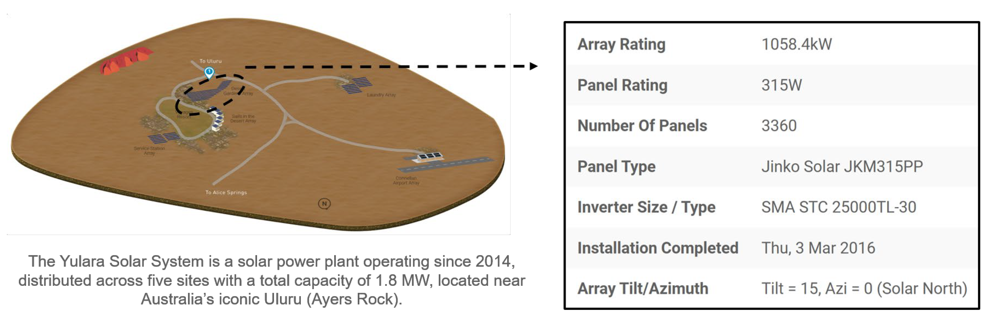
The Desert Knowledge Australia Solar Center (DKASC) in Alice Springs, Australia, provided the historic PV energy data used in this study. This information can be freely accessed at [24] and is part of a public dataset. The Alice Springs, Yulara, and NT solar power plants are part of the DKASC center. A solar power facility made up of five sites plus a weather station is called the Yulara Solar System. Therefore, the data is selected from No.1 (1058.4 kW, poly-Si, Fixed, 2016, Desert Gardens) at Yulara Solar System in this study. Its location is shown in Figure 1.

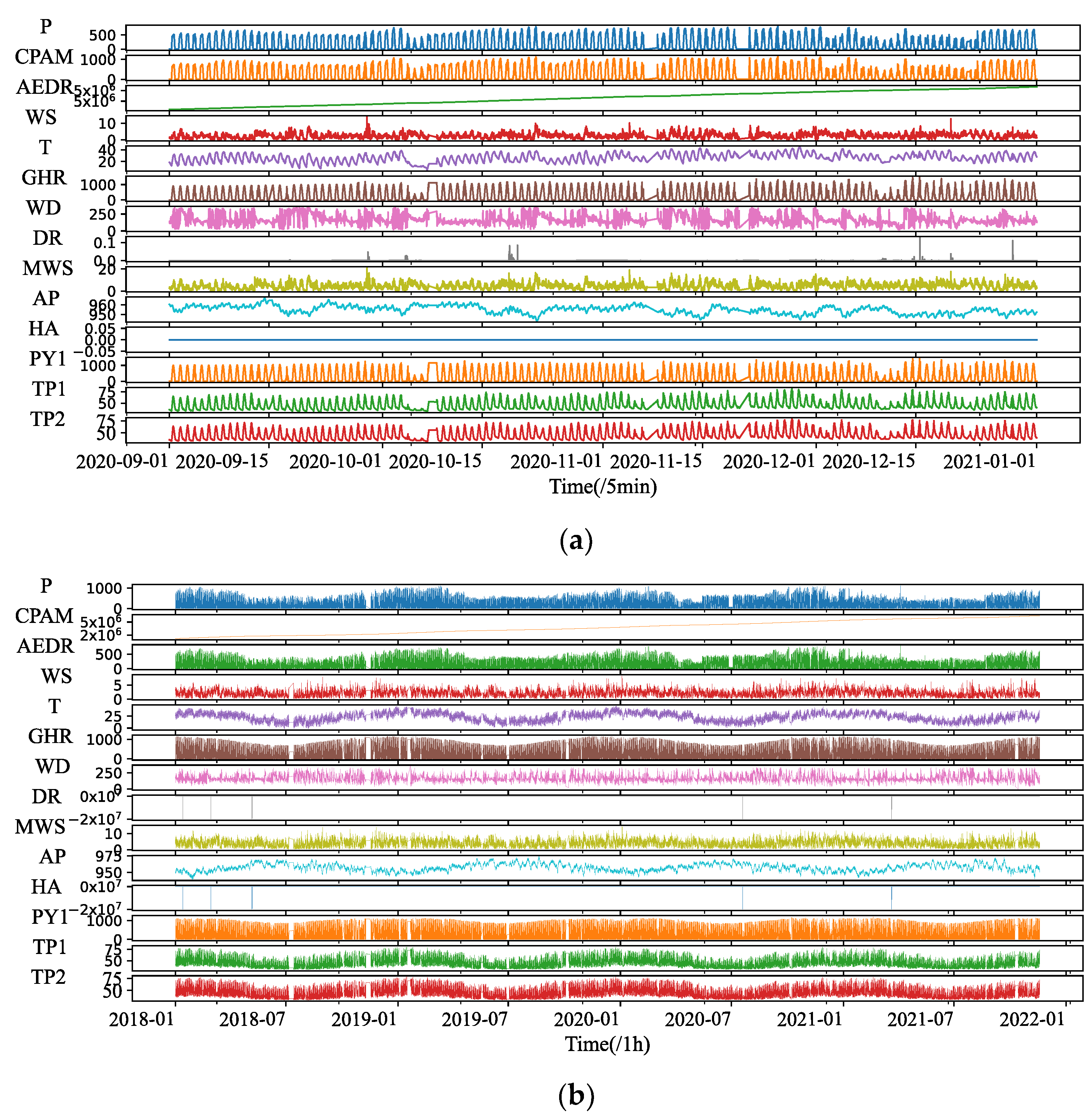
The total installed capacity of the PV system is 1058.4 kW, and both the historical power data and the weather data have a 5 min time precision. The historical data set includes Active Power (P), Wind Speed (WS), Wind Direction (WD), Weather Temperature Celsius (T), Weather Daily Rainfall (DR), Global Horizontal Radiation (GHR), Max Wind Speed (MWS), Air Pressure (AP), Hail Accumulation (HA), Pyranometer 1(PY1), Temperature Probe 1 and 2 (TP1&TP2).

We use two datasets for the proposed models to learn, including the 4 months power data with a resolution of 5 min, from 1 September 2020 to 31 December 2020, a total of 34,080 samples, and the 4 years PV power data with a resolution of 1 h, from 2017 to 2020, a total of 33,740 samples. Figure 2 displays the historic PV time series of two datasets, where the label of the vertical axis is the abbreviation of all variable names in the data set, and the horizontal axis represents the length of the time step of the data set.

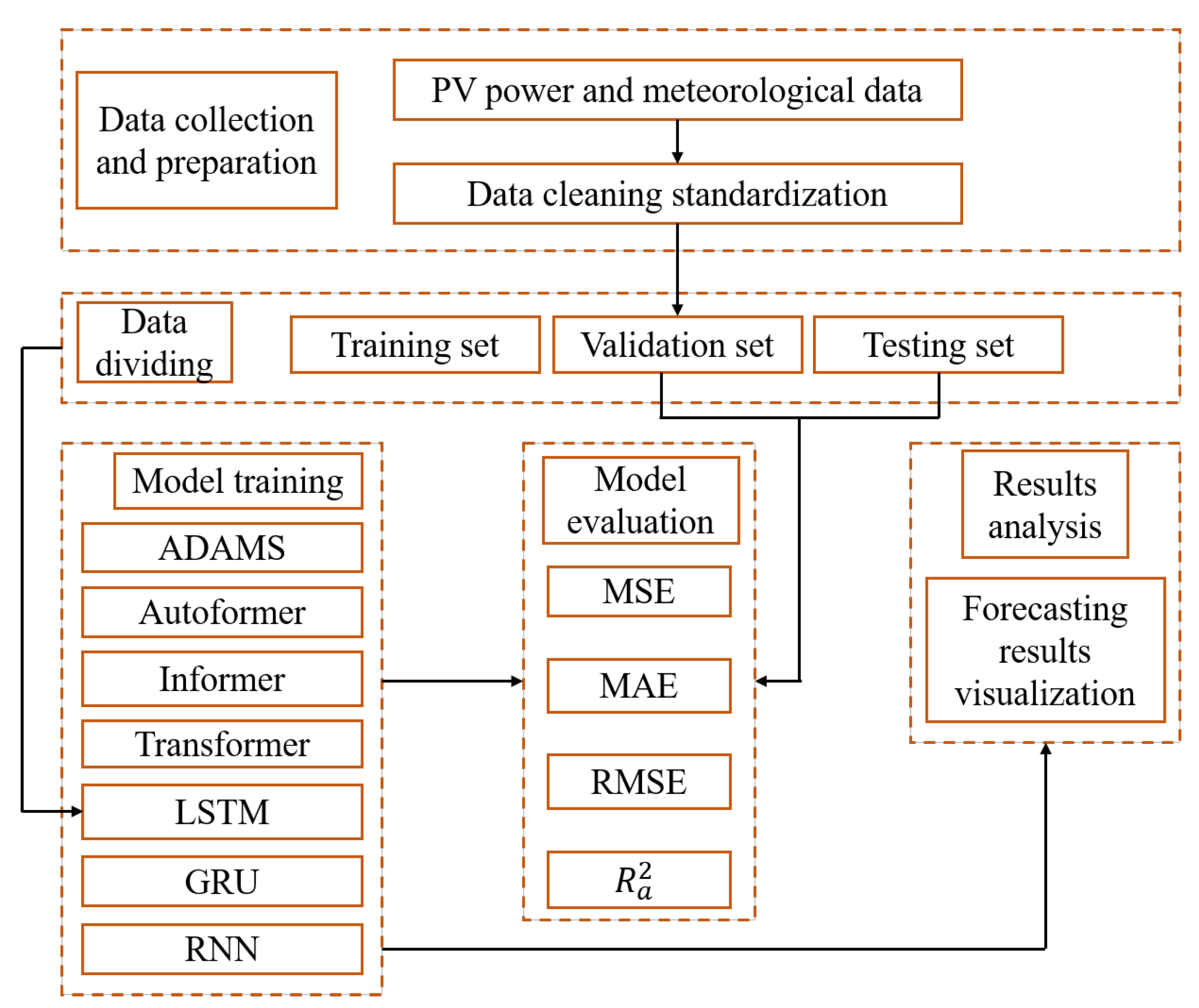
4.2. Experimental Framework

ADAMS and six other experimental competitive models are suggested in this work. Autoformer, Informer, Transformer, LSTM, GRU, and RNN are the baseline models. Data collection, data preparation, data dividing, model training, model evaluation, and results analysis are all included in the fundamental building blocks of STPVF. Figure 3 depicts the entire experimental flow diagram, and

Table 1. The parameters for each model.

Model	Parameters
ADAMS	$d_{model}=512,seq\_len=24,pre\_len=\left(4,8,12,24\right),itr=1,$ $Train\_epochs=5,learn\_rate=0.0001,dropout=0.05$ $label\_len=12,batchsize=64,loss\_function=adaptive,$
Autoformer	$d_{model}=512, seq\_len=24,pre\_len=\left(4,8,12,24\right),itr=1,$ $Train\_epochs=5,learn\_rate=0.0001,dropout=0.05,$ $label\_len=12,batchsize=64,loss\_function=mse$
Informer	$d_{model}=512, seq\_len=24,pre\_len=\left(4,8,12,24\right),itr=1,$ $Train\_epochs=5,learn\_rate=0.0001,dropout=0.05,$ $label\_len=12,batchsize=64,loss\_function=mse$
Transformer	$d_{model}=512, seq\_len=24,pre\_len=\left(4,8,12,24\right),itr=1,$ $Train\_epochs=5,learn\_rate=0.0001,dropout=0.05$ $label\_len=12,batchsize=64,loss\_function=mse$
LSTM	$seq\_len=24,pre\_len=\left(4,8,12,24\right),batchsize=64,$ $Train\_epochs=100,learn\_rate=0.0001,$ $dropout=0.05,loss\_function=mse$
GRU	$seq\_len=24,pre\_len=\left(4,8,12,24\right),batchsize=64,$ $Train\_epochs=100,learn\_rate=0.0001,$ $dropout=0.05,loss\_function=mse$
RNN	$seq\_len=24,pre\_len=\left(4,8,12,24\right),batchsize=64,$ $Train\_epochs=100,learn\_rate=0.0001,$ $dropout=0.05,loss\_function=mse$

includes a list of the parameter settings for models like the ADAMS.

4.3. Data Pre-Processing

The initial step of study involves the collection and pre-processing of data. The data needs to be preprocessed to ensure the performance of our model. Due to maintenance issues or device failure, there are occasional cases where data is missing. The chosen datasets are then processed by deleting any negative numbers for electricity generation and interpolating any existing missing values. For a variety of reasons, the dataset was divided into three sections. The training set, validation set, and test set each make up 70%, 20%, and 10% of the datasets, respectively.

4.4. Evaluation Metrics

Four different evaluation indices, including Mean Square Error (MSE), Mean Absolute Error (MAE), Root Mean Square Error (RMSE), and adjusted R-squared ($R_a^2$), were utilized to assess the performance of the models in this study. These are their expressions:

$$\begin{array}{c}\mathrm{MSE}=\frac{1}{N}{\displaystyle \sum _{t=1}^N}{\left(p_t-{\widehat{p}}_t\right)}^2\end{array}$$

(18)

$$\begin{array}{c}\mathrm{MAE}=\frac{1}{N}{\displaystyle \sum _{t=1}^N}\left|p_t-{\widehat{p}}_t\right|\end{array}$$

(19)

$$\begin{array}{c}\mathrm{RMSE}=\sqrt{\frac{1}{N}{\displaystyle \sum _{t=1}^N}{\left(p_t-{\widehat{p}}_t\right)}^2}\end{array}$$

(20)

$$\begin{array}{c}{R}^2=1-\frac{{\sum }_t{\left(p_t-{\widehat{p}}_t\right)}^2}{{\sum }_t{\left(p_t-{\overline{p}}_t\right)}^2}\end{array}$$

(21)

$$R_a^2=1-\frac{n-1}{n-k-1}\left(1-R^2\right)$$

(22)

where $N$ is the amount of PV energy sample points utilized to calculate the prediction error, $p_t$ is the actual PV power values, ${\overline{p}}_{\mathrm{t} }$ is the mean of the prediction period taken into consideration, and ${\widehat{p}}_t$ is the predicted values. MSE is a frequently employed metric to assess the efficacy of time series forecasting. In this paper, all baseline models used the MSE as a loss function. The real circumstance of the error between the forecasting value and the actual value can be better reflected by MAE because it is less sensitive to outliers. RMSE is prone to high values and accentuates the distance between significant mistakes. Better performance is indicated by these indicators’ lower levels.$R^2$ denotes R-squared and it represents the percentage of variance that the model accounts for and displays the correlation between forecasted and actual values. By considering the effects of additional independent factors that have a propensity to distort the outcomes of $R^2$ measurements, $R_a^2$, a modified form of $R^2$, increases accuracy and reliability. Its value ranges from 0 to 1. The lager value of this indicator means better performance.

5. Experiment and Analysis

The PV power forecasting results of the suggested model and six baseline models are summarized and analyzed in this section. In this study, forecasting is conducted in four different prediction lengths (4, 8, 12 and 24) using data with a 5 min precision as well as data with an hourly resolution. Since the epoch periods of the seven models used in the experiments of this work differ significantly, additional convergence parameters, for instance the speed of loss converge of the seven models trained under the datasets, are not compared. In this research, each forecasting approach is implemented using Python 3.8, which runs on a computer with 12th Intel(R) Xeon(R) Platinum 8255C CPU 2.5 GHz 43 GB and NVIDIA GeForce RTX 3080 GPU 12 GB.

5.1. Experiment I: 5-min PV Power Forecasting Experiment

On the 5 min resolution dataset, we contrast and examine the suggested model with the other six models. In the experiment, obviously, the suggested model has performed uniformly the best of all the models.

Table 2. PV power forecasting accuracy evaluation of 5 min.

	Metrics	ADAMS	Autoformer	Informer	Transformer	LSTM	GRU	RNN
4	MSE	0.061	0.116	0.076	0.063	0.234	0.190	0.146
	MAE	0.146	0.166	0.178	0.120	0.284	0.296	0.234
	RMSE	0.248	0.341	0.276	0.252	0.484	0.436	0.382
	$R_a^2$	0.940	0.886	0.925	0.938	0.835	0.822	0.863
8	MSE	0.074	0.205	0.129	0.083	0.290	0.184	0.216
	MAE	0.134	0.247	0.226	0.188	0.315	0.323	0.301
	RMSE	0.273	0.453	0.359	0.289	0.538	0.429	0.464
	$R_a^2$	0.927	0.799	0.874	0.918	0.795	0.828	0.797
12	MSE	0.099	0.143	0.130	0.122	0.262	0.324	0.140
	MAE	0.164	0.226	0.229	0.222	0.303	0.409	0.248
	RMSE	0.315	0.378	0.355	0.349	0.512	0.569	0.374
	$R_a^2$	0.903	0.860	0.876	0.880	0.815	0.697	0.869
24	MSE	0.173	0.215	0.255	0.214	0.297	0.389	0.324
	MAE	0.227	0.288	0.322	0.301	0.332	0.469	0.400
	RMSE	0.416	0.464	0.505	0.462	0.545	0.624	0.569
	$R_a^2$	0.831	0.788	0.750	0.790	0.789	0.636	0.776

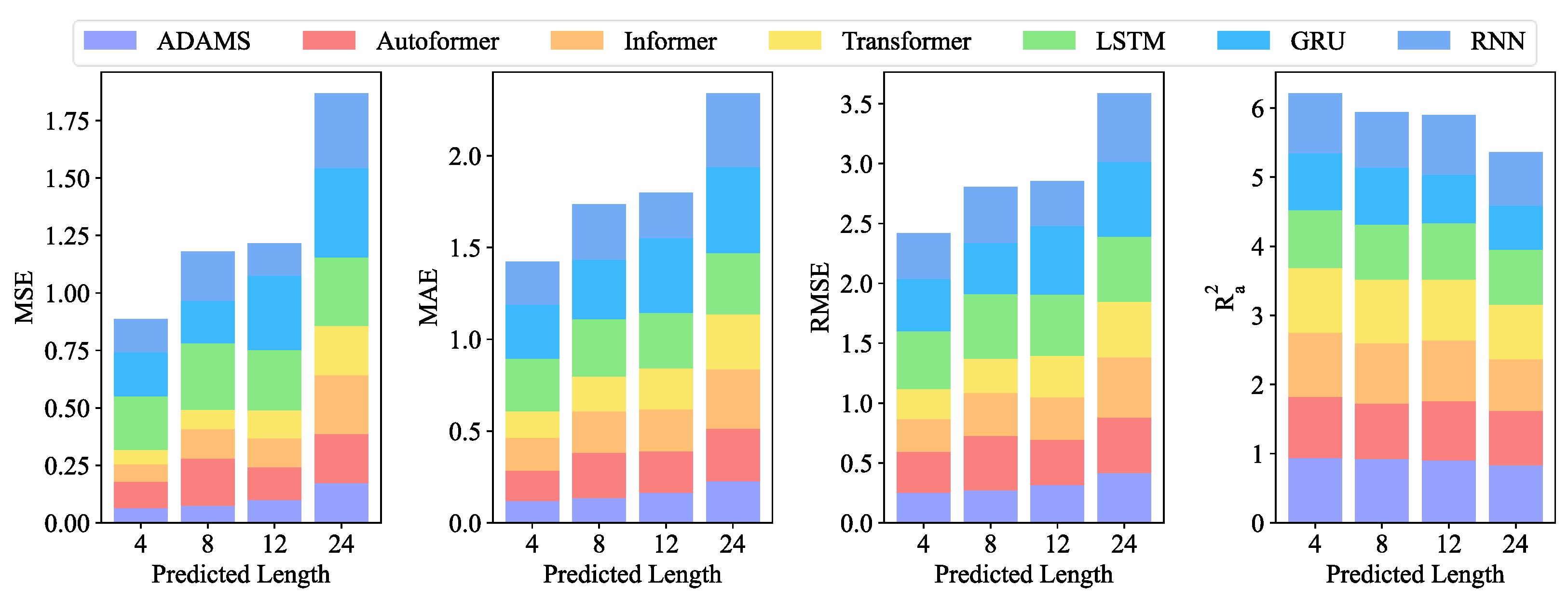
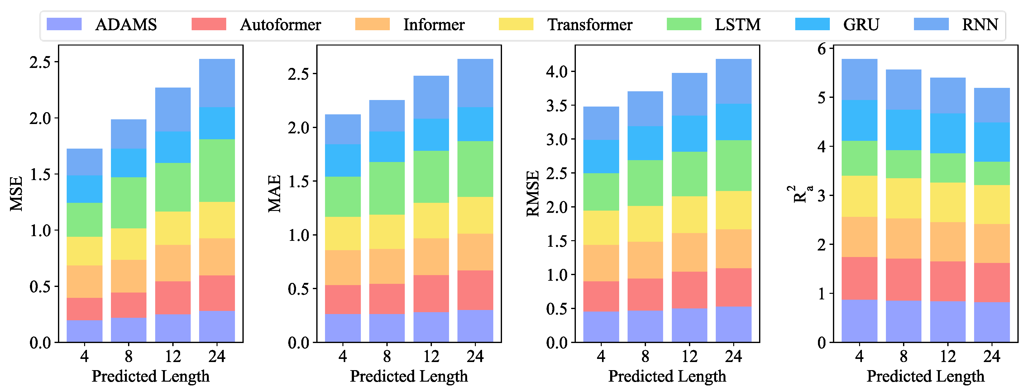
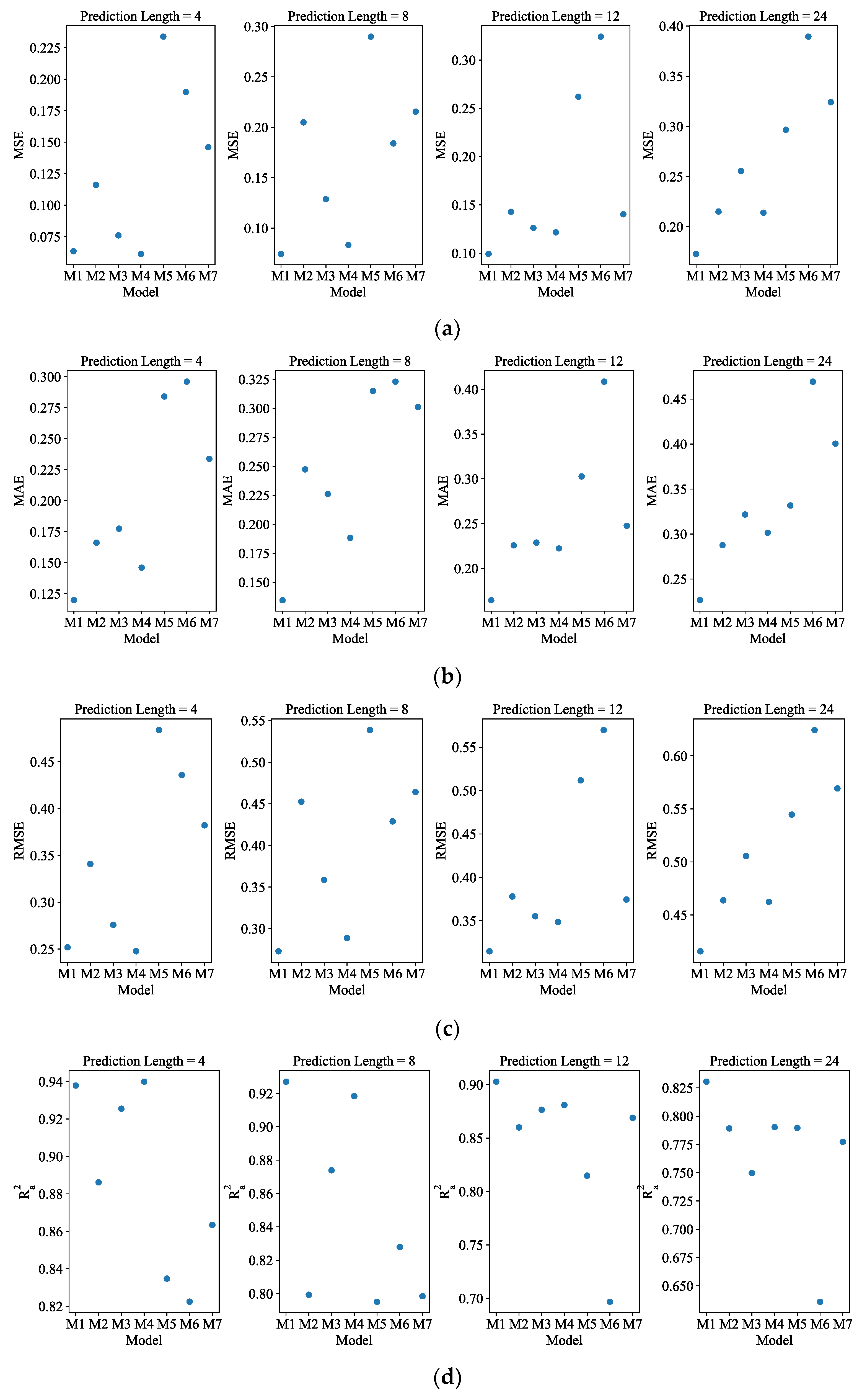
lists the thorough analyses of the predicted outcomes. Figure 4 displays the visual bar chart. Figure A1 shows the visual scatter plot. According to Table 2, ADAMS achieved the best MSE of 0.061 in the forecasting of length-4, whereas Autoformer, Informer, Transformer, LSTM, GRU, and RNN achieved MSEs of 0.116, 0.076, 0.063, 0.304, 0.190, and 0.146, respectively. As can be observed from Figure 4, when the forecasting interval is extended to length-24, the prediction errors for most competing approaches worsen. The suggested model exhibits better predicting performance for all four forecasting lengths within 120 min for data with a 5 min resolution. The prediction precision of all models exhibits a general tendency of declining with increasing length.

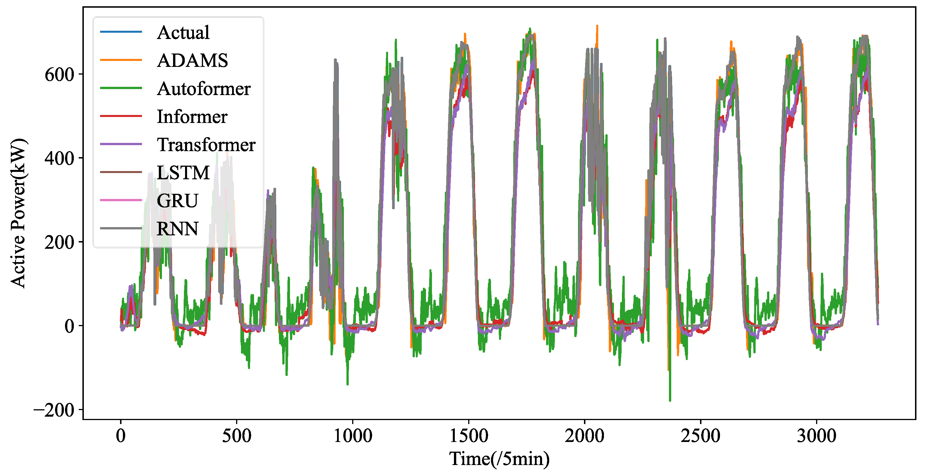
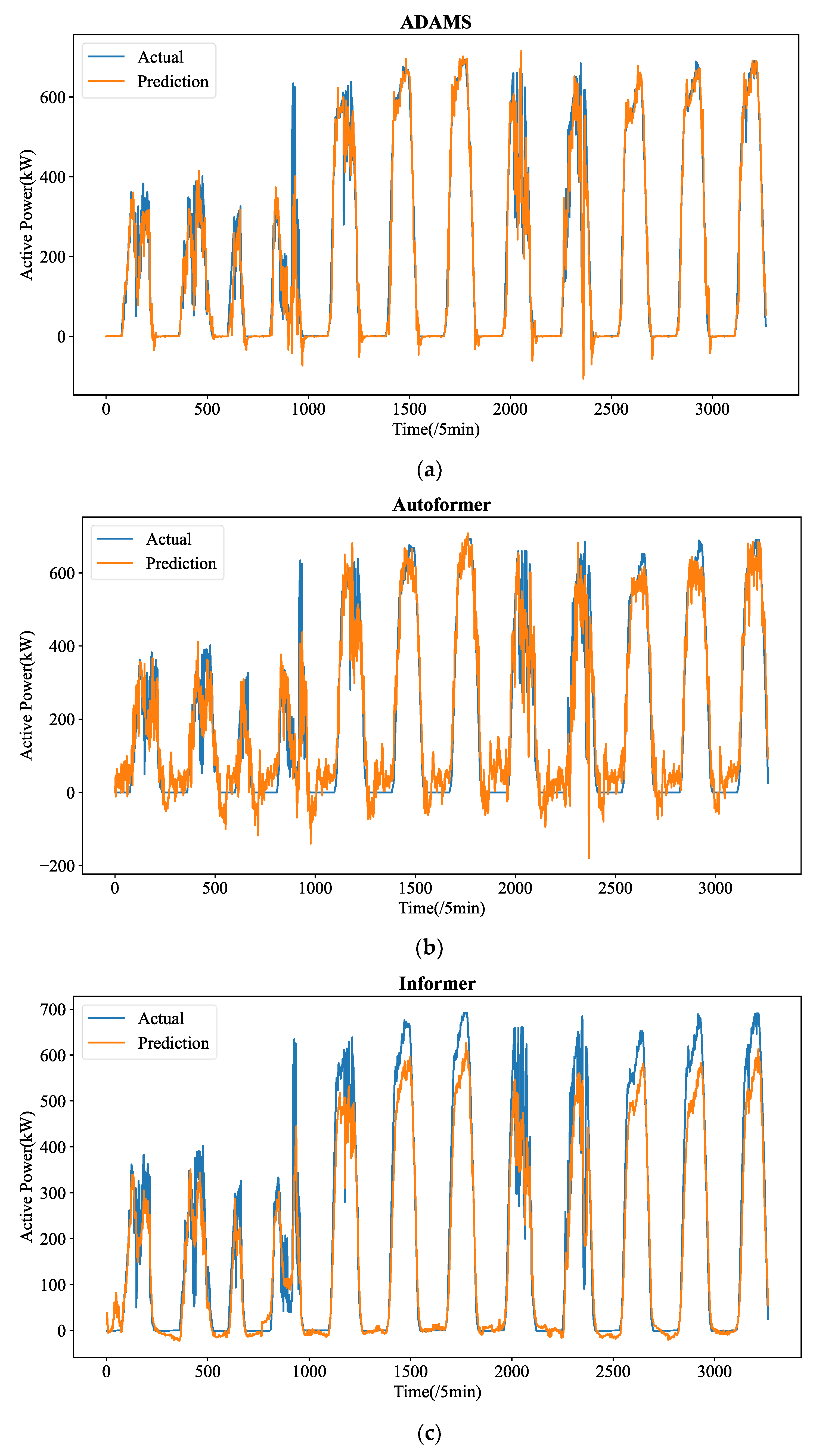
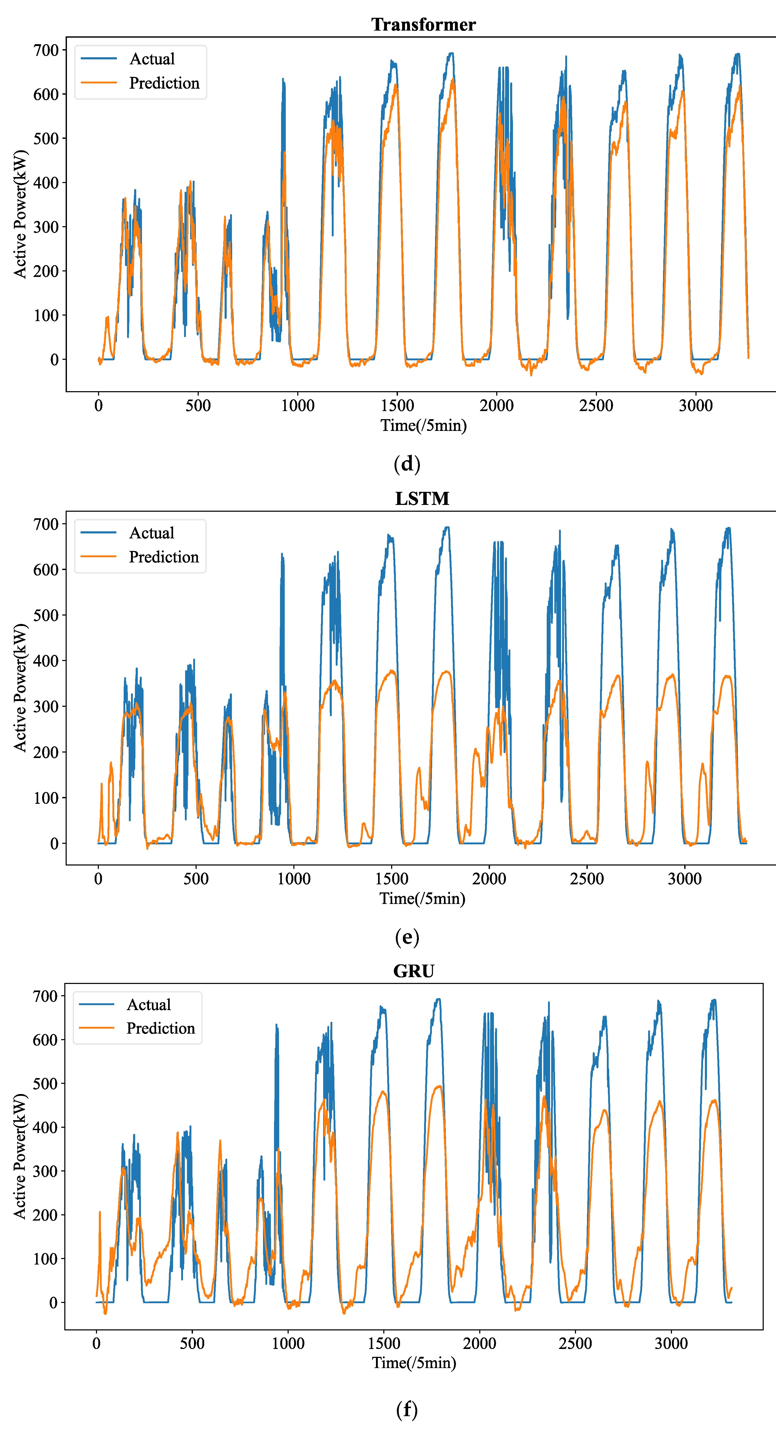
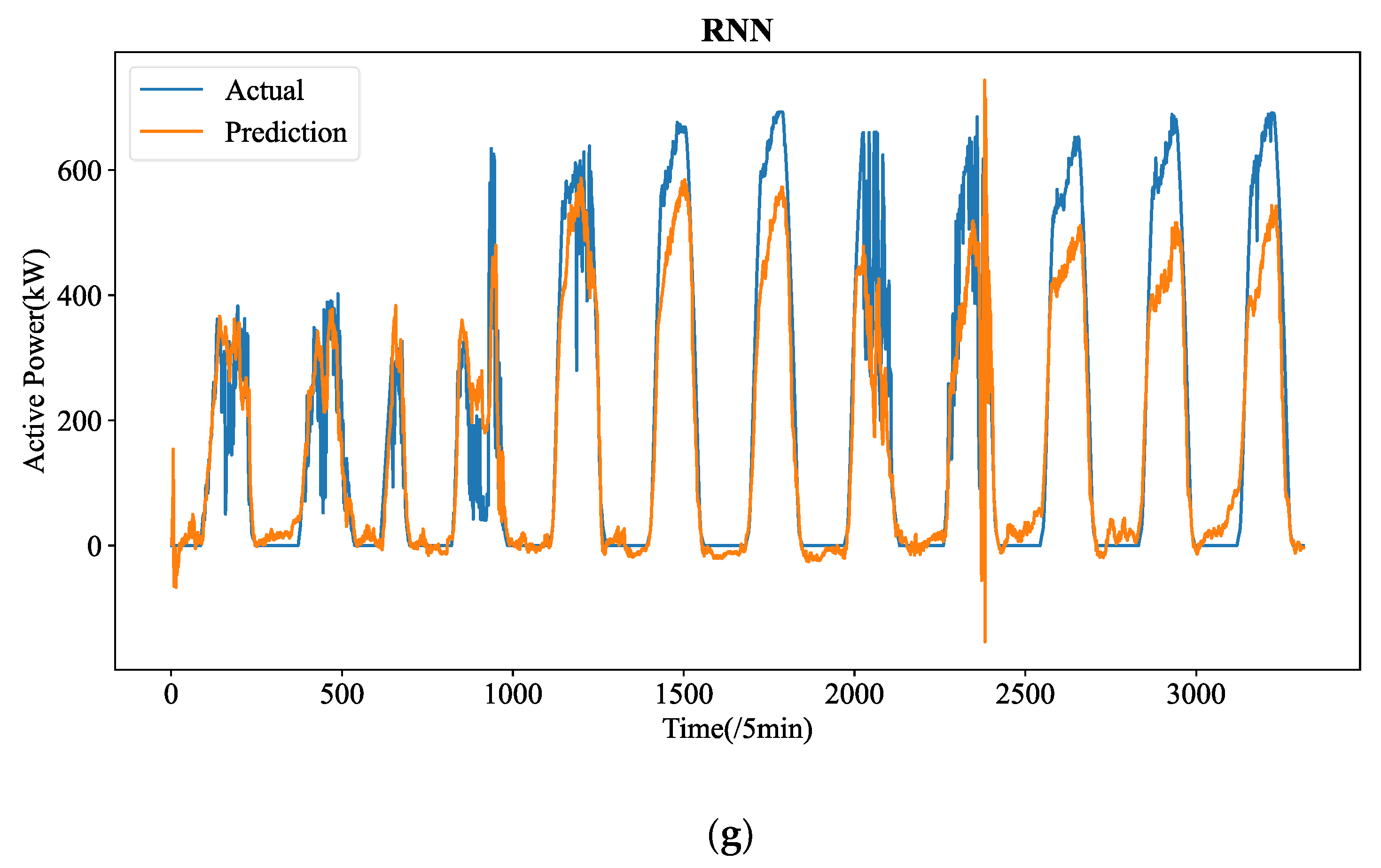
Figure 5 shows the forecasting curves of all models for the length-24 forecasting results. The forecasting curves of each model are shown in Figure A3. We can observe that ADAMS is also proved to be the most successful model in reconstructing the fluctuation details. One-step prediction models, e.g., LSTM, GRU, and RNN are frequently used; multi-step prediction procedures will cause significant error accumulation issues. In particular, the prediction mistake from the earlier forecasting would accrue in the upcoming forecast, adding significant forecasting bias and leading to much higher MSE. Additionally, the PV power data patterns are very intricate. Their ability to learn historical details will be severely hampered by the limited computer memory. They cannot effectively learn global patterns in their memory cell without a heuristic selection process. Instead, they are only able to recall patterns in extremely small ranges, which could interfere with forecasting. The four transformer-based prediction models perform well in terms of accuracy. Too many variations have been predicted by models such as LSTM and RNN, which is referred to as the overfitting phenomena. The approximate fluctuation curves have been effectively reconstructed by Autoformer, Informer, and Transformer, however certain crucial elements have not been precisely predicted. In contrast, ADAMS accurately restores a number of significant information, including minor variations and turning points, which constitute the better understanding of the time series.

Therefore, even if the datasets exhibit extremely fluctuating patterns, the suggested ADAMS is adept at projecting PV power time series over the very short-term (5 min resolution) and recovering the precise fluctuation tendencies. Additionally, the suggested ADAMS has generated an excellent result that can serve as a fresh baseline in future research on STPVF. Although ADAMS outperforms competing approaches in our comparative trials, we did not compare ADAMS to competing approaches because, according to earlier research, ADAMS outperforms rival approaches in forecasting.

5.2. Experiment II: Hourly PV Power Forecasting Experiment

The forecasting precision of each experimental model is examined using hourly PV power data to supply more conclusive evidence of the efficacy of our suggested ADAMS. In

Table 3. PV power forecasting accuracy evaluation of 1 h.

	Metrics	ADAMS	Autoformer	Informer	Transformer	LSTM	GRU	RNN
4	MSE	0.197	0.201	0.289	0.255	0.304	0.244	0.237
	MAE	0.265	0.268	0.322	0.311	0.373	0.284	0.276
	RMSE	0.455	0.448	0.537	0.505	0.551	0.494	0.487
	$R_a^2$	0.873	0.870	0.816	0.840	0.716	0.827	0.832
8	MSE	0.219	0.227	0.292	0.279	0.457	0.254	0.257
	MAE	0.265	0.282	0.325	0.320	0.490	0.299	0.291
	RMSE	0.468	0.476	0.540	0.528	0.676	0.504	0.507
	$R_a^2$	0.856	0.857	0.816	0.825	0.573	0.820	0.818
12	MSE	0.251	0.294	0.325	0.297	0.431	0.280	0.389
	MAE	0.283	0.343	0.344	0.329	0.485	0.318	0.396
	RMSE	0.501	0.542	0.570	0.545	0.657	0.540	0.624
	$R_a^2$	0.842	0.815	0.794	0.813	0.597	0.807	0.725
24	MSE	0.280	0.319	0.330	0.323	0.560	0.284	0.428
	MAE	0.302	0.369	0.340	0.342	0.518	0.301	0.444
	RMSE	0.529	0.564	0.574	0.569	0.748	0.532	0.654
	$R_a^2$	0.824	0.799	0.793	0.796	0.476	0.800	0.697

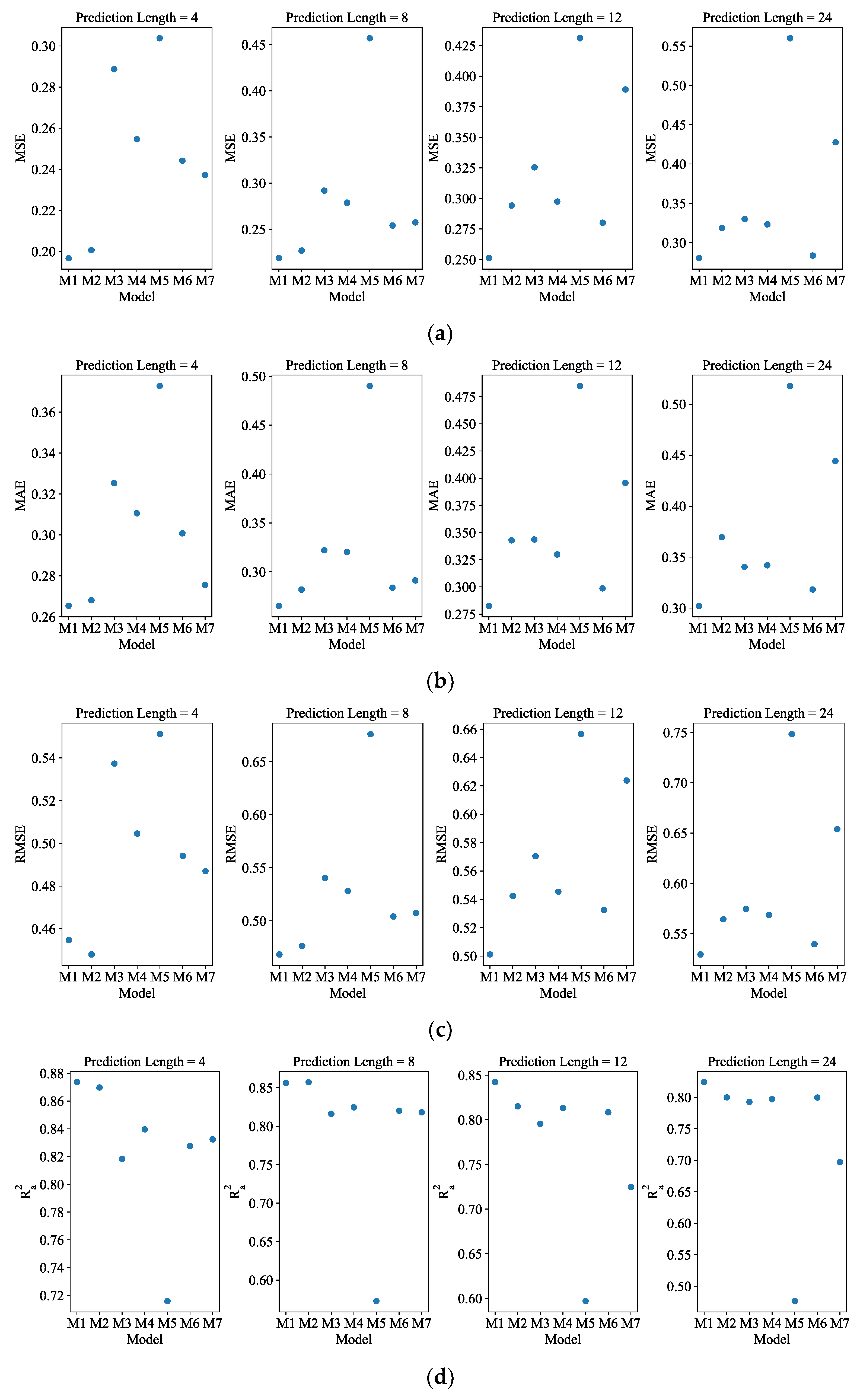
, Figure 6 and Figure A2, an error evaluation, a visual bar chart and a visual scatter plot are shown, respectively. Among all the models available, the ADAMS is still the model that performs the best, according to Table 3. For all of the lengths in advance, ADAMS has the maximum number of the four evaluation indexes best values, as shown in Table 3, while Autoformer and GRU each account for one. Additionally, ADAMS displays the best values across all evaluation indexes for all future lengths. It is important to note that LSTM predicts the curve poorly, with MSE values of 0.304, 0.457, 0.431, and 0.560 being the highest. For hourly resolution of data, the ADAMS model exhibits better predicting performance for all four pre-lengths throughout a day, as shown in Figure 6 which displays the forecasting outcomes of all models. The prediction accuracy of all models has a general declining trend with increasing length, similarly to the Exp. I.

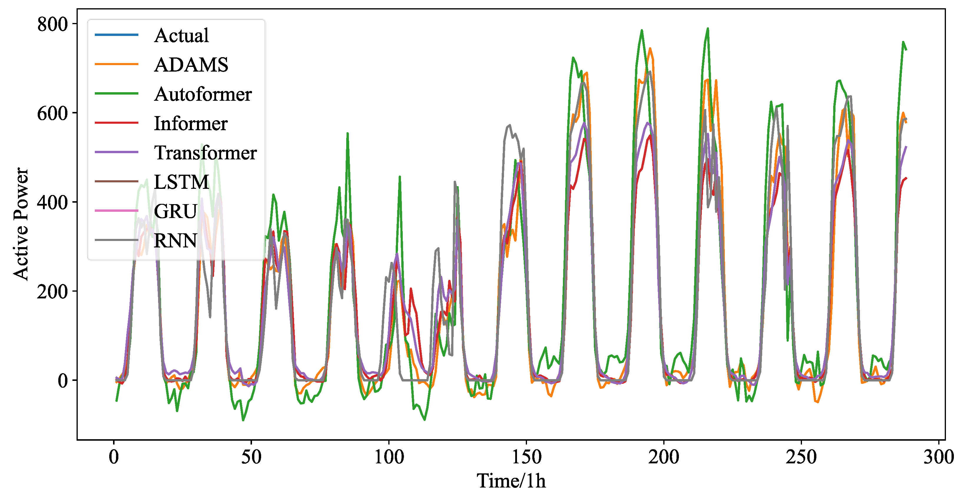
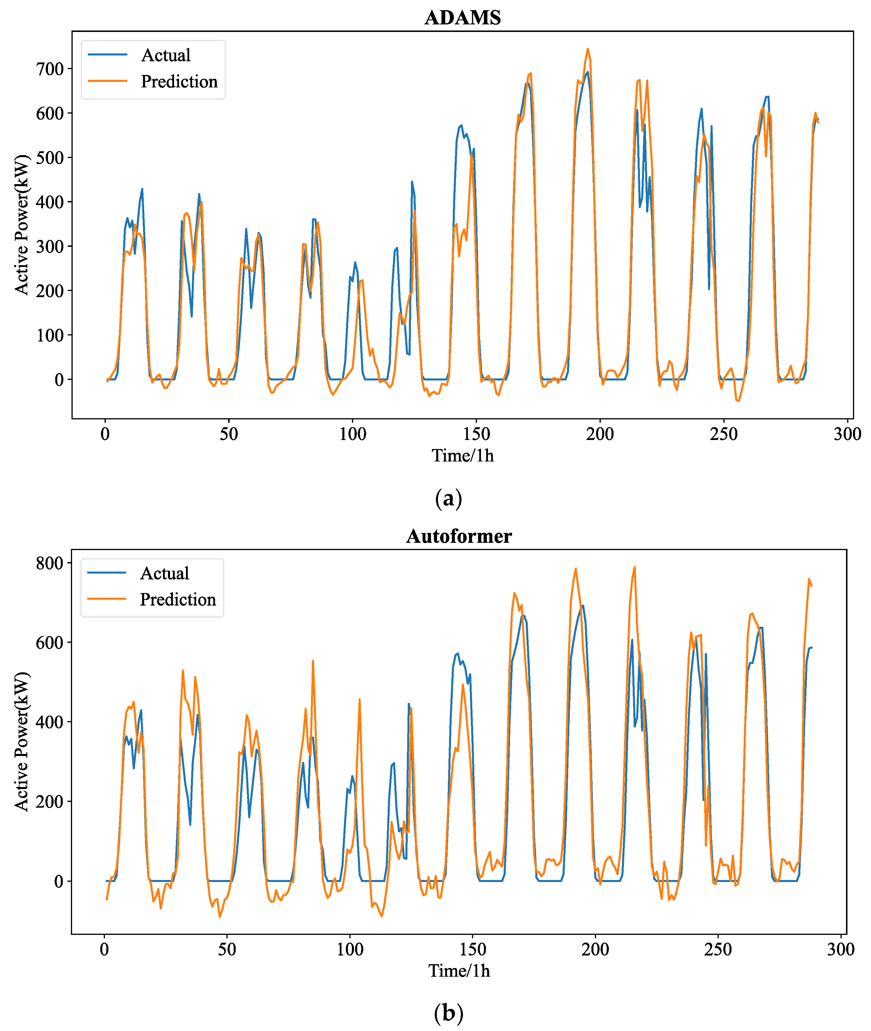
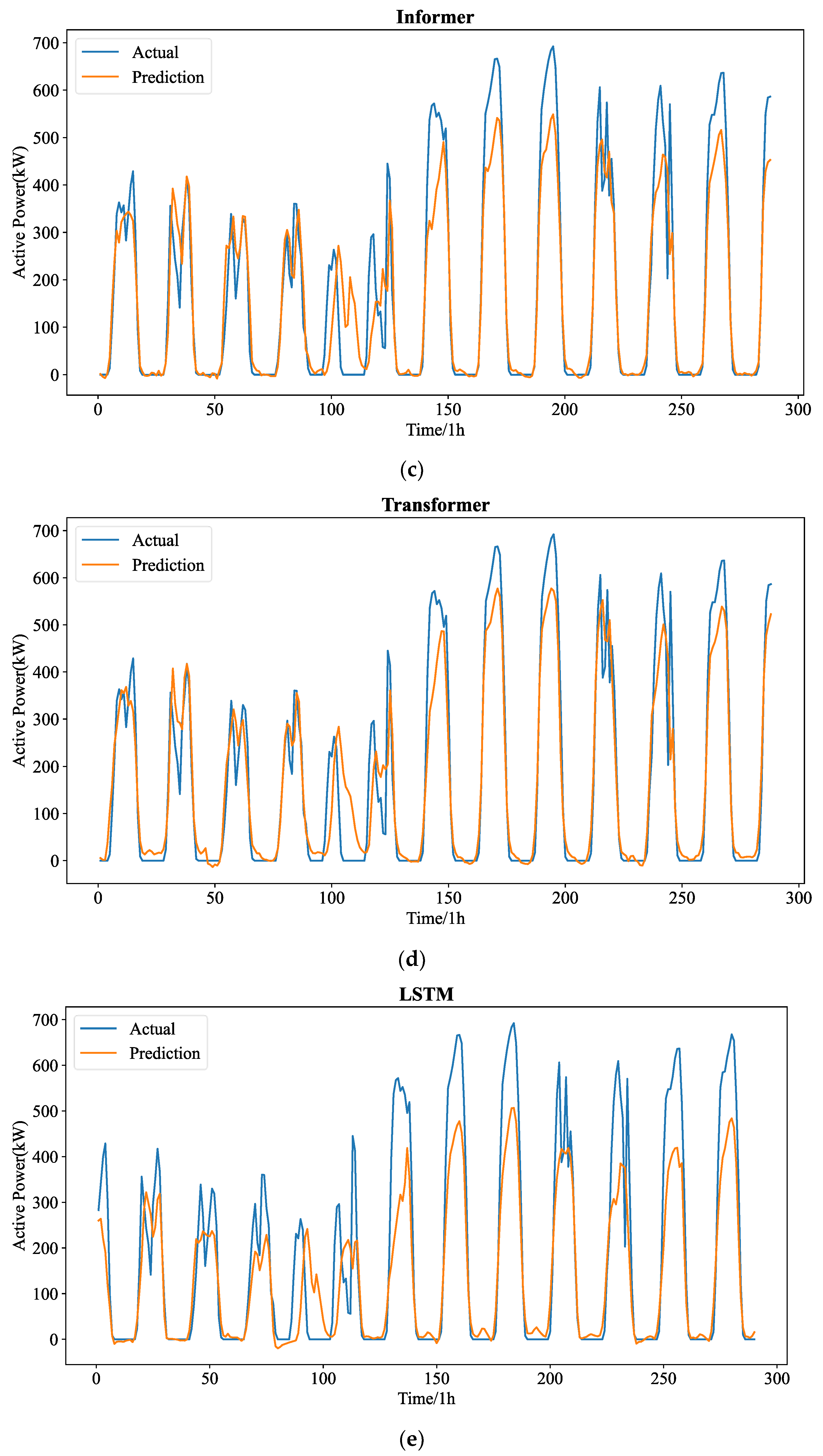
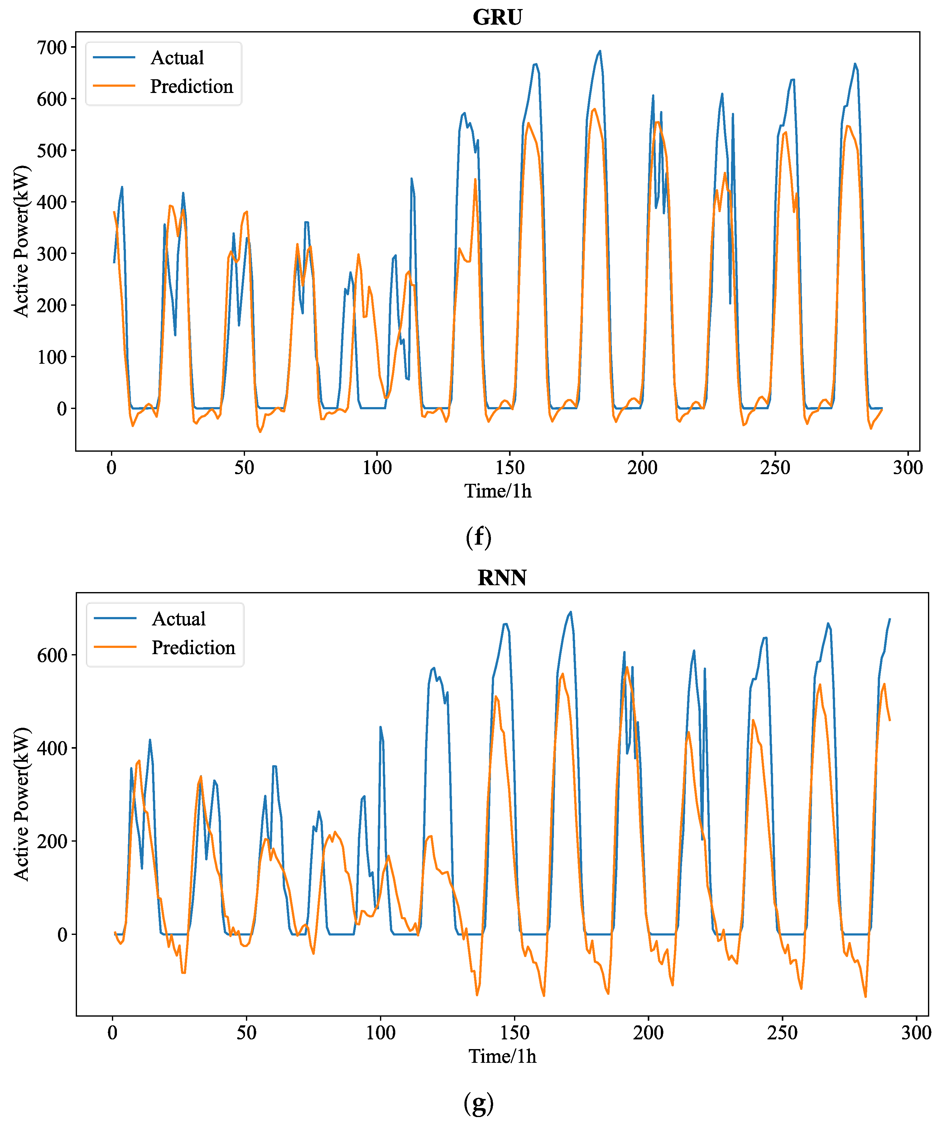
Figure 7 shows the forecasting curves of all models for the length-24 forecasting results. The forecasting curves of each model are shown in Figure A4. It can be seen that the hourly PV statistics are more consistent and less randomly erratic than the 5 min PV data. However, the predicting curves of all models reveal that 5 min resolution data are more favorable to good forecasting performance. This depends on the temporal properties of the PV power time series themselves, and as resolution rises, so does the number of historical values that can be used for forecasting.

When comparing Exp. I and Exp. II, we can find that the ranges of $R_a^2$ for the hourly resolution data and the 5 min resolution data for all lengths of seven models are 0.476 to 0.873 and 0.636 to 0.940, respectively. The forecasting of length-4 shows the highest $R_a^2$ for both resolutions, while the length-12 and length-24 show the lowest $R_a^2$. As observed from the aforementioned, the quality of fit of the model decreases with increasing pre-length on the two resolution datasets. The quality of fit of the model is better in the higher resolution (5 min resolution) data set. The complete range of the predicted PV power can be explained by the suggested model in 0.824 to 0.938. As seen from the aforementioned, on both resolution data sets, the quality of fit of the model increases with increasing resolution, with the 5 min resolution data set having the best fit. On both resolution data sets, the goodness of fit of the model decreases with increasing predicted length.

5.3. Diebold-Mariano Test

In order to evaluate the null hypothesis on the difference in accuracy between two forecasting models, Diebold and Mariano proposed explicit tests [25,26]. Model prediction errors can be non-Gaussian, non-zero-mean, serially correlated, and contemporaneously correlated, and the loss function is not required to be quadratic or symmetric [25]. The strength of ADAMS is not overwhelming to Autoformer and Transformer, as shown in Table 2 and Table 3. The Diebold-Mariano test are run as a result to perform more research.

Let $H_0$ be the null hypothesis, which states that there is no difference in prediction accuracy between the two models. $H_1$ be the alternative hypothesis, which states that the prediction accuracy between the two models is obviously different. MSE is the loss function used in this hypothesis test. If the p-value is higher than 0.05, there is no difference. $H_1$ will be allowed if p-value is less than 0.05.

Table A1. The outcomes of the Diebold-Mariano test (5 min resolution data).

	Models	ADAMS	Autoformer	Informer	Transformer	LSTM	GRU	RNN
4	ADAMS	0.00 × 10+00	4.89 × 10−02	1.37 × 10−02	1.30 × 10−12	1.39 × 10−133	1.13 × 10−235	1.00 × 10−292
	Autoformer	4.89 × 10−02	0.00 × 10+00	9.01 × 10−07	8.26 × 10−24	5.84 × 10−135	1.74 × 10−232	1.07 × 10−280
	Informer	1.37 × 10−02	9.01 × 10−07	0.00 × 10+00	3.38 × 10−28	3.61 × 10−156	2.08 × 10−289	0.00 × 10+00
	Transformer	1.30 × 10−12	8.26 × 10−24	3.38 × 10−28	0.00 × 10+00	6.14 × 10−156	3.70 × 10−289	0.00 × 10+00
	LSTM	0.00 × 10+00	0.00 × 10+00	0.00 × 10+00	0.00 × 10+00	0.00 × 10+00	4.98 × 10−93	1.01 × 10−171
	GRU	0.00 × 10+00	0.00 × 10+00	0.00 × 10+00	0.00 × 10+00	4.98 × 10−93	0.00 × 10+00	1.70 × 10−61
	RNN	0.00 × 10+00	0.00 × 10+00	0.00 × 10+00	0.00 × 10+00	1.01 × 10−171	1.70 × 10−61	0.00 × 10+00
8	ADAMS	0.00 × 10+00	9.78 × 10−75	3.27 × 10−58	6.80 × 10−03	2.61 × 10−42	0.00 × 10+00	0.00 × 10+00
	Autoformer	9.78 × 10−75	0.00 × 10+00	5.81 × 10−25	1.12 × 10−74	6.05 × 10−01	0.00 × 10+00	0.00 × 10+00
	Informer	3.27 × 10−58	5.81 × 10−25	0.00 × 10+00	0.00 × 10+00	1.37 × 10−45	0.00 × 10+00	0.00 × 10+00
	Transformer	6.80 × 10−03	1.12 × 10−74	0.00 × 10+00	0.00 × 10+00	3.46 × 10−48	0.00 × 10+00	0.00 × 10+00
	LSTM	0.00 × 10+00	0.00 × 10+00	0.00 × 10+00	0.00 × 10+00	0.00 × 10+00	0.00 × 10+00	0.00 × 10+00
	GRU	0.00 × 10+00	2.91 × 10−123	0.00 × 10+00	0.00 × 10+00	0.00 × 10+00	0.00 × 10+00	3.21 × 10−35
	RNN	0.00 × 10+00	1.58 × 10−274	0.00 × 10+00	0.00 × 10+00	0.00 × 10+00	3.21 × 10−35	0.00 × 10+00
12	ADAMS	0.00 × 10+00	3.00 × 10−109	5.20 × 10−02	7.14 × 10−01	1.32 × 10−191	1.48 × 10−10	3.42 × 10−253
	Autoformer	3.00 × 10−109	0.00 × 10+00	6.72 × 10−131	2.07 × 10−114	2.60 × 10−139	5.26 × 10−21	2.84 × 10−248
	Informer	5.20 × 10−02	6.72 × 10−131	0.00 × 10+00	3.50 × 10−07	0.00 × 10+00	6.73 × 10−09	1.35 × 10−223
	Transformer	7.14 × 10−01	2.07 × 10−114	3.50 × 10−07	0.00 × 10+00	0.00 × 10+00	4.59 × 10−04	0.00 × 10+00
	LSTM	0.00 × 10+00	0.00 × 10+00	0.00 × 10+00	0.00 × 10+00	0.00 × 10+00	0.00 × 10+00	0.00 × 10+00
	GRU	0.00 × 10+00	0.00 × 10+00	0.00 × 10+00	0.00 × 10+00	0.00 × 10+00	0.00 × 10+00	0.00 × 10+00
	RNN	0.00 × 10+00	2.92 × 10−193	0.00 × 10+00	0.00 × 10+00	0.00 × 10+00	0.00 × 10+00	0.00 × 10+00
24	ADAMS	0.00 × 10+00	1.67 × 10−03	7.54 × 10−185	1.26 × 10−07	0.00 × 10+00	0.00 × 10+00	0.00 × 10+00
	Autoformer	1.67 × 10−03	0.00 × 10+00	2.19 × 10−163	2.25 × 10−02	0.00 × 10+00	0.00 × 10+00	0.00 × 10+00
	Informer	7.54 × 10−185	2.19 × 10−163	0.00 × 10+00	0.00 × 10+00	0.00 × 10+00	0.00 × 10+00	4.88 × 10−293
	Transformer	1.26 × 10−07	2.25 × 10−02	0.00 × 10+00	0.00 × 10+00	0.00 × 10+00	0.00 × 10+00	0.00 × 10+00
	LSTM	0.00 × 10+00	0.00 × 10+00	0.00 × 10+00	0.00 × 10+00	0.00 × 10+00	2.50 × 10−02	0.00 × 10+00
	GRU	0.00 × 10+00	0.00 × 10+00	0.00 × 10+00	0.00 × 10+00	2.50 × 10−02	0.00 × 10+00	0.00 × 10+00
	RNN	0.00 × 10+00	0.00 × 10+00	4.88 × 10−293	0.00 × 10+00	0.00 × 10+00	0.00 × 10+00	0.00 × 10+00

and

Table A2. The outcomes of the Diebold-Mariano test (hourly resolution data).

	Models	ADAMS	Autoformer	Informer	Transformer	LSTM	GRU	RNN
4	ADAMS	0.00 × 10+00	6.89 × 10−03	1.41 × 10−109	1.48 × 10−56	0.00 × 10+00	0.00 × 10+00	0.00 × 10+00
	Autoformer	6.89 × 10−03	0.00 × 10+00	2.55 × 10−135	1.44 × 10−80	0.00 × 10+00	0.00 × 10+00	0.00 × 10+00
	Informer	1.41 × 10−109	2.55 × 10−135	0.00 × 10+00	9.37 × 10−81	0.00 × 10+00	0.00 × 10+00	0.00 × 10+00
	Transformer	1.48 × 10−56	1.44 × 10−80	9.37 × 10−81	0.00 × 10+00	0.00 × 10+00	0.00 × 10+00	0.00 × 10+00
	LSTM	0.00 × 10+00	0.00 × 10+00	0.00 × 10+00	0.00 × 10+00	0.00 × 10+00	9.18 × 10−01	5.54 × 10−02
	GRU	0.00 × 10+00	0.00 × 10+00	0.00 × 10+00	0.00 × 10+00	9.18 × 10−01	0.00 × 10+00	1.19 × 10−01
	RNN	0.00 × 10+00	0.00 × 10+00	0.00 × 10+00	0.00 × 10+00	5.54 × 10−02	1.19 × 10−01	0.00 × 10+00
8	ADAMS	0.00 × 10+00	2.02 × 10−12	2.60 × 10−222	1.38 × 10−214	3.19 × 10−141	8.17 × 10−62	5.39 × 10−133
	Autoformer	2.02 × 10−12	0.00 × 10+00	1.18 × 10−290	7.43 × 10−288	1.19 × 10−194	6.69 × 10−123	1.98 × 10−179
	Informer	2.60 × 10−222	1.18 × 10−290	0.00 × 10+00	3.87 × 10−06	1.94 × 10−21	2.07 × 10−97	9.84 × 10−02
	Transformer	1.38 × 10−214	7.43 × 10−288	3.87 × 10−06	0.00 × 10+00	2.99 × 10−13	1.11 × 10−77	8.22 × 10−01
	LSTM	3.19 × 10−141	1.19 × 10−194	1.94 × 10−21	2.99 × 10−13	0.00 × 10+00	7.97 × 10−44	4.68 × 10−07
	GRU	8.17 × 10−62	6.69 × 10−123	2.07 × 10−97	1.11 × 10−77	7.97 × 10−44	0.00 × 10+00	5.75 × 10−34
	RNN	5.39 × 10−133	1.98 × 10−179	9.84 × 10−02	8.22 × 10−01	4.68 × 10−07	5.75 × 10−34	0.00 × 10+00
12	ADAMS	0.00 × 10+00	2.20 × 10−221	0.00 × 10+00	1.46 × 10−121	0.00 × 10+00	0.00 × 10+00	0.00 × 10+00
	Autoformer	2.20 × 10−221	0.00 × 10+00	8.02 × 10−96	6.72 × 10−09	0.00 × 10+00	0.00 × 10+00	0.00 × 10+00
	Informer	0.00 × 10+00	8.02 × 10−96	0.00 × 10+00	0.00 × 10+00	0.00 × 10+00	0.00 × 10+00	0.00 × 10+00
	Transformer	1.46 × 10−121	6.72 × 10−09	0.00 × 10+00	0.00 × 10+00	0.00 × 10+00	0.00 × 10+00	0.00 × 10+00
	LSTM	0.00 × 10+00	0.00 × 10+00	0.00 × 10+00	0.00 × 10+00	0.00 × 10+00	1.14 × 10−150	4.54 × 10−185
	GRU	0.00 × 10+00	0.00 × 10+00	0.00 × 10+00	0.00 × 10+00	1.14 × 10−150	0.00 × 10+00	0.00 × 10+00
	RNN	0.00 × 10+00	0.00 × 10+00	0.00 × 10+00	0.00 × 10+00	4.54 × 10−185	0.00 × 10+00	0.00 × 10+00
24	ADAMS	0.00 × 10+00	0.00 × 10+00	0.00 × 10+00	2.18 × 10−172	0.00 × 10+00	0.00 × 10+00	0.00 × 10+00
	Autoformer	0.00 × 10+00	0.00 × 10+00	9.87 × 10−08	3.20 × 10−95	0.00 × 10+00	0.00 × 10+00	0.00 × 10+00
	Informer	0.00 × 10+00	9.87 × 10−08	0.00 × 10+00	0.00 × 10+00	0.00 × 10+00	0.00 × 10+00	0.00 × 10+00
	Transformer	2.18 × 10−172	3.20 × 10−95	0.00 × 10+00	0.00 × 10+00	0.00 × 10+00	0.00 × 10+00	0.00 × 10+00
	LSTM	0.00 × 10+00	0.00 × 10+00	0.00 × 10+00	0.00 × 10+00	0.00 × 10+00	6.16 × 10−03	0.00 × 10+00
	GRU	0.00 × 10+00	0.00 × 10+00	0.00 × 10+00	0.00 × 10+00	6.16 × 10−03	0.00 × 10+00	0.00 × 10+00
	RNN	0.00 × 10+00	0.00 × 10+00	0.00 × 10+00	0.00 × 10+00	0.00 × 10+00	0.00 × 10+00	0.00 × 10+00

display the outcomes of the Diebold-Mariano test. As a result, it can be shown that p-value is never greater than 0.05, proving that the PV power calculated by the ADAMS is substantially more accurate than that of the other models under comparison.

5.4. Ablation Study

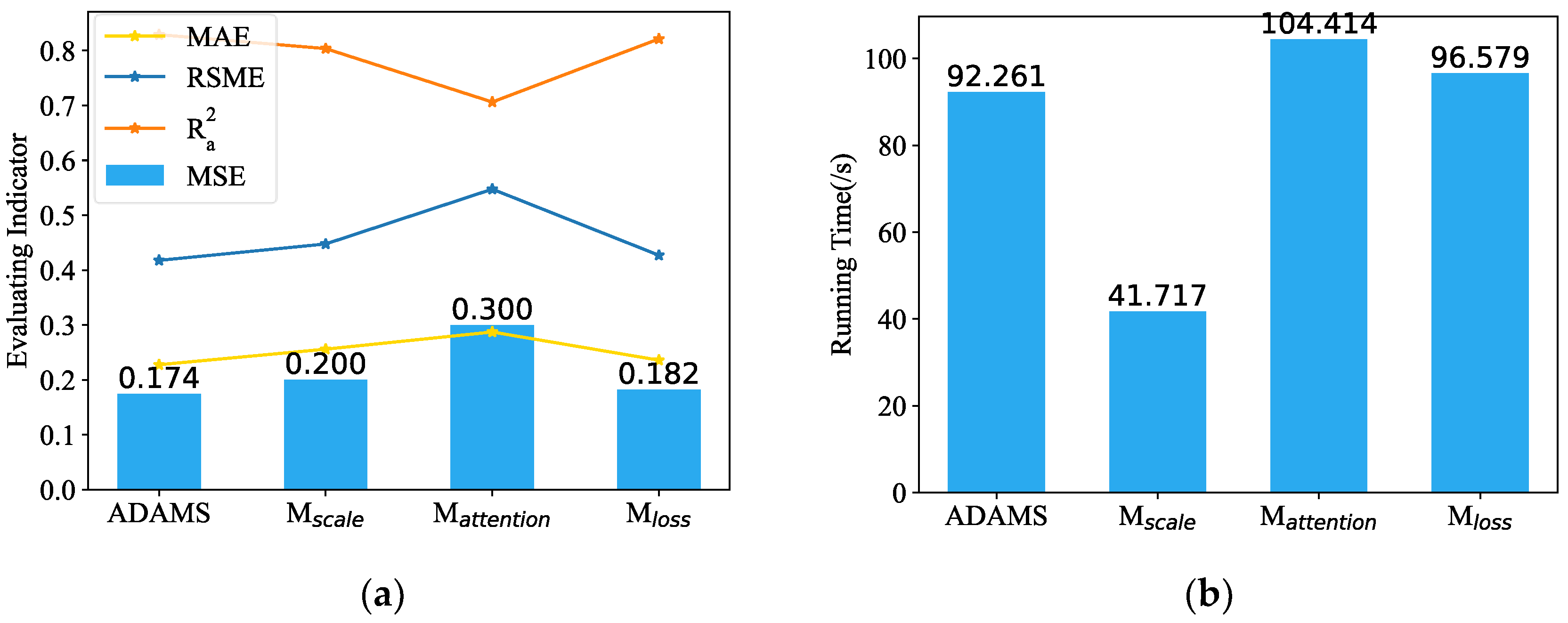
We used Exp.1 (length-24) to conduct ablation research to confirm the effects of various improvement measures in the ADAMS model. The multi-scale framework, the de-stationary attention module, and the adaptive loss function (replaced by MSE), respectively, are removed from ADAMS via the $M_{scale}$, $M_{atttention}$, and $M_{loss}$ functions.

According to Figure 8, the MSE increases to 1.72 times when the $M_{atttention}$ is utilized, showing that the de-stationary attention significantly improves the objectivity and dependability of the outcome prediction. The removal of the multi-scale module shortens training time but increases MSE by 4.598%. When the adaptive loss function was applied in place of the MSE, the MSE increased by 14.943% while the training time increased a little. Three other evaluation indicators also show a similar situation. The statistical results demonstrate that the proposed ADAMS model, which incorporates all performance enhancement techniques, performs best, and that the most effective performance enhancement technique for ADAMS accuracy is de-stationary attention, followed by multi-scale framework and adaptive loss function.

5.5. Further Study

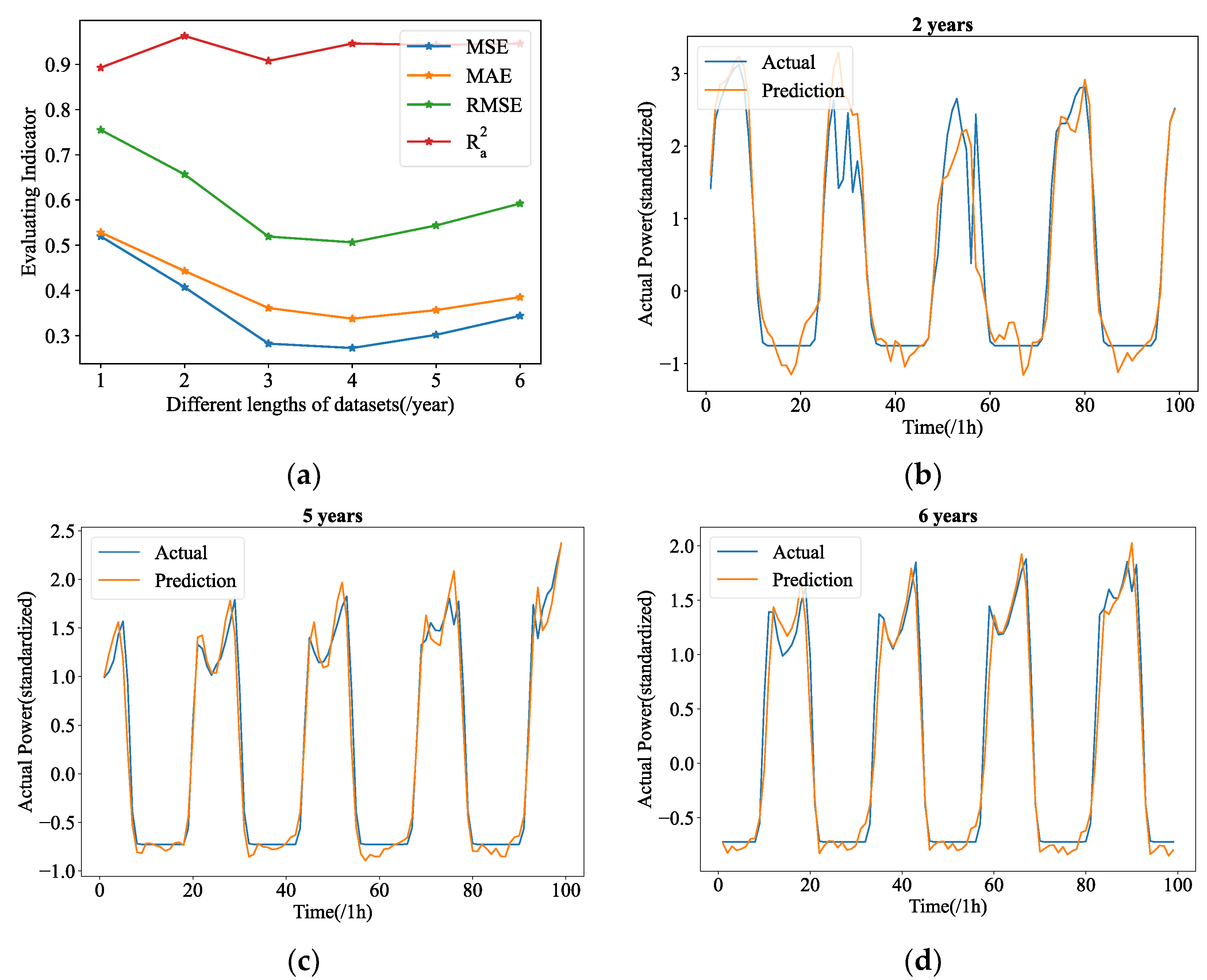
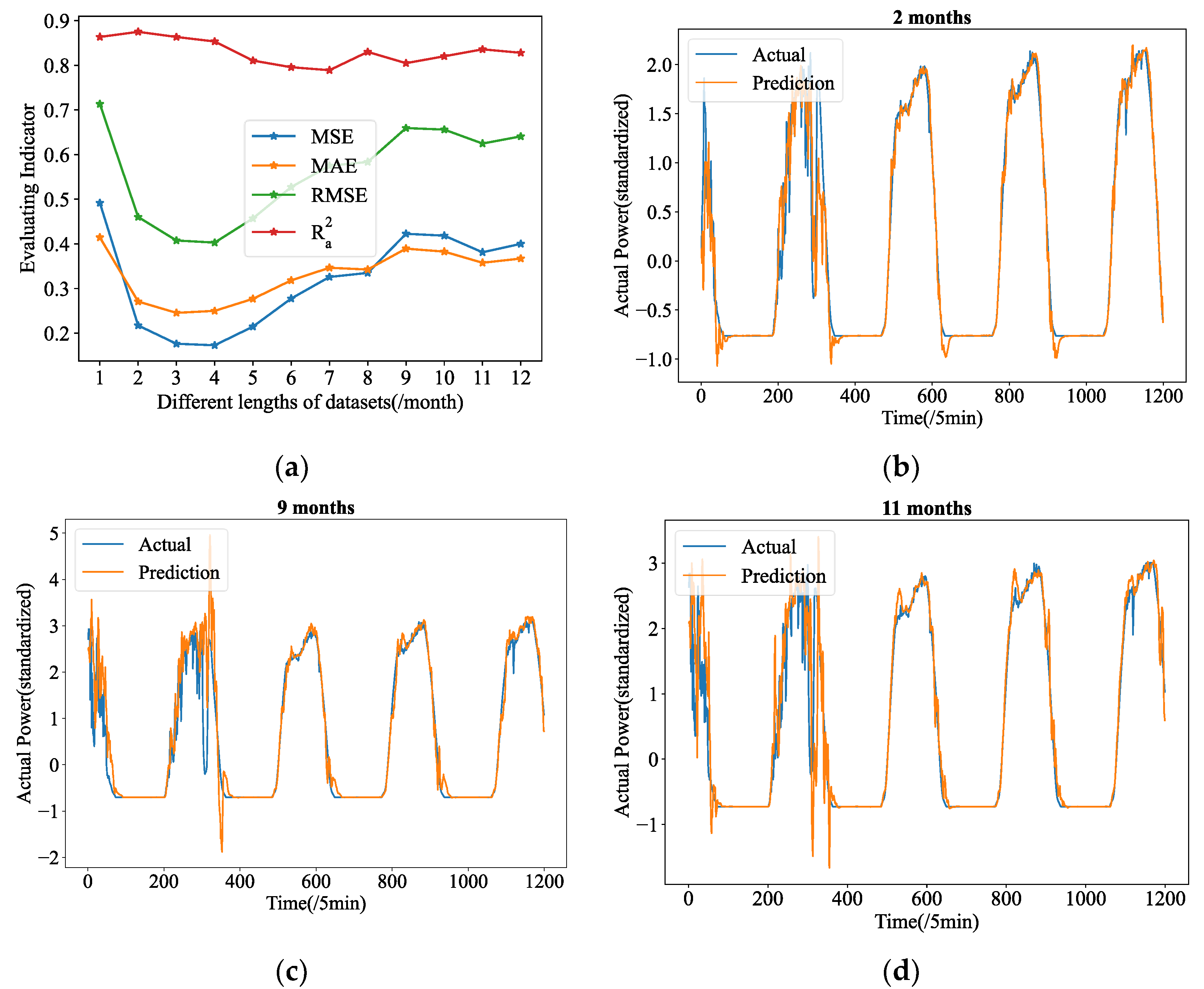
It makes sense that the longer the training time series, the more knowledge the models can pick up, resulting in a better forecasting outcome. The longer training datasets, it turns out, may not necessarily result in a forecast that is more correct. On the other hand, longer series datasets underperformed, with greater MSE, MAE, RMSE, and lower $R_a^2$. Further studies are conducted as a result, in which we built up 12 experimental groups with PV power data of the 5 min resolution data provided by Yulara Solar System, ranging in duration from 1 month to 12 months. Additionally, six experimental groups are set up collecting data with hourly resolution ranging from one year to six years. In these experiments, their forecasting tasks are fixed at length-24 in advance. Figure 9a and Figure 10a display the four evaluation indicators from various experimental groups of 5 min and hourly resolution data, respectively. As seen in Figure 9a, the total MSE has witnessed a rising trend as dataset lengths have increased to a given value, with the lowest points occurring at lengths of 4 months. As shown in Figure 10a, the lowest point of MSE appears at the length of 4 years. Therefore, the 4 months datasets (5 min resolution) and 4 years datasets (hourly resolution) are those we used for this study.

It is interesting to note that some experimental groups with longer datasets even exhibit overfitting during testing, defying the conventional wisdom that more data will help to reduce overfitting in deep learning. In Figure 9b–d, the forecasting outcomes of the 2 months, 9 months, and 11 months datasets are depicted. Evidently, for the two-month datasets, the insufficient PV power data makes it quite natural for models to overfit the training data. When there is insufficient data, as shown in Figure 9, the predicted curve shows obvious error compared with the real curve. The predicting curves of 9 months and 11 months, when the time series data are considerably longer than 2 months, however, shows greater fluctuation, and even has several serious errors. This makes them much more inconsistent with the ground truth patterns. As for the hourly resolution data, additional data is required to fully understand this phenomenon, however the Yulara Solar system currently only has six years’ worth of data.

It is quite difficult to provide sufficient proof in a very short amount of time due to the inadequate data. This work presented two ideas for our future research in STPVF based on this peculiar phenomenon:

• Due to the global use of self-attention and auto-correlation while training, if the time series is too lengthy, they will likely be dispersed to some historical data from the distant past that is unrelated to the current trends. The current PV power in STPVF only roughly correlates to the prior trend over a narrow range. Therefore, the historical PV power from a long time ago could seriously impair auto-correlation or self-attention.
• Because the long-ago historical data disturbs the auto-correlation if the previous historic patterns resemble strikingly the current ones, the parallel historic patterns may lead the model to incorrectly predict the current trend based on the parallel historic patterns. That is to say, the forecasting errors have increased because the model has overfitted the past time series.

6. Conclusions

A novel neural network model is suggested in this paper to address the STPVF. This research suggested the ADAMS, in which the additional de-stationary attention is introduced in both the encoder and decoder modules, to find specific time dependencies based on the complete sequence information before the stationary, to resolve the extreme fluctuations and irregular trends of STPVF data. In order to find the time dependent patterns in long history data, Autoformer also utilized a multi-scale framework with a cross-scale normalization method. ADAMS and other competitive models are used to perform STPVF, using the Yulara Solar System in Central Australia as the case study. The experiment exhibits the suggested ADAMS’s capacity to foresee frequent variations as well as to extract deeper information from extremely erratic data patterns. It is important to note that, in contrast to earlier studies, the suggested ADAMS produced an excellent result in STPVF. This work also performed an experiment of the STPVF based on the hourly resolution PV power dataset to further demonstrate the superiority of the proposed ADAMS. The additional case study also offers compelling proof that ADAMS excels at deep knowledge learning and restores crucial information even from slicker data. Additionally, the proposed ADAMS was versatile, and besides the exogenous variables used in this paper for PV energy prediction, other exogenous variables can be used. Moreover, it is able to adapt to time series with different characteristics, and it can be used for forecasting tasks in other fields in future research.

Although most studies have shown that adding more data helps to solve the overfitting issue, in the area of STPVF, a larger time series dataset for learning may not be able to better predict future PV power. Two possibilities are put out in response to this counterintuitive phenomenon. On the one hand, larger datasets could disperse the auto-correlation to ancient historical time series from a long time ago. On the other hand, the model may be led astray to overfit the historical data by the dispersed auto-correlation. Future research will focus on providing a strict demonstration of the proposed assumptions and determining the ideal duration of the training datasets for STPVF.

References

- Kabir, E.; Kumar, P.; Kumar, S.; Adelodun, A.A.; Kim, K.-H. Solar energy: Potential and future prospects. Renew. Sustain. Energy Rev. 2018, 82, 894–900. [Google Scholar] [CrossRef]
- Creutzig, F.; Agoston, P.; Goldschmidt, J.C.; Luderer, G.; Nemet, G.; Pietzcker, R.C. The underestimated potential of solar energy to mitigate climate change. Nat. Energy 2017, 2, 1–9. [Google Scholar] [CrossRef]
- Stein, G.; Letcher, T.M. 15—Integration of PV Generated Electricity into National Grids. In A Comprehensive Guide to Solar Energy Systems; Letcher, T.M., Fthenakis, V.M., Eds.; Academic Press: Cambridge, MA, USA, 2018; pp. 321–332. [Google Scholar]
- Cervone, G.; Clemente-Harding, L.; Alessandrini, S.; Delle Monache, L. Short-term photovoltaic power forecasting using Artificial Neural Networks and an Analog Ensemble. Renew. Energy 2017, 108, 274–286. [Google Scholar] [CrossRef]
- Agoua, X.G.; Girard, R.; Kariniotakis, G. Short-Term Spatio-Temporal Forecasting of Photovoltaic Power Production. IEEE Trans. Sustain. Energy 2018, 9, 538–546. [Google Scholar] [CrossRef]
- Wu, H.; Xu, J.; Wang, J.; Long, M. Autoformer: Decomposition Transformers with Auto-Correlation for Long-Term Series Forecasting. Adv. Neural Inf. Process. Syst. 2021, 34, 22419–22430. [Google Scholar]
- Pan, M.; Li, C.; Gao, R.; Huang, Y.; You, H.; Gu, T.; Qin, F. Photovoltaic power forecasting based on a support vector machine with improved ant colony optimization. J. Clean. Prod. 2020, 277, 123948. [Google Scholar] [CrossRef]
- Zhou, Y.; Zhou, N.; Gong, L.; Jiang, M. Prediction of photovoltaic power output based on similar day analysis, genetic algorithm and extreme learning machine. Energy 2020, 204, 117894. [Google Scholar] [CrossRef]
- Zhang, C.; Peng, T.; Nazir, M.S. A novel integrated photovoltaic power forecasting model based on variational mode decomposition and CNN-BiGRU considering meteorological variables. Electr. Power Syst. Res. 2022, 213, 108796. [Google Scholar] [CrossRef]
- He, Y.; Gao, Q.; Jin, Y.; Liu, F. Short-term photovoltaic power forecasting method based on convolutional neural network. Energy Rep. 2022, 8, 54–62. [Google Scholar] [CrossRef]
- Ghannay, S.; Favre, B.; Estève, Y.; Camelin, N. Word Embedding Evaluation and Combination. In Proceedings of the Tenth International Conference on Language Resources and Evaluation (LREC′16), Portorož, Slovenia, 23–28 May 2016; European Language Resources Association (ELRA): Portorož, Slovenia, 2016; pp. 300–305. [Google Scholar]
- Vaswani, A.; Shazeer, N.; Parmar, N.; Uszkoreit, J.; Jones, L.; Gomez, A.N.; Kaiser, L.; Polosukhin, I. Attention Is All You Need. Adv. Neural Inf. Process. 2017. [Google Scholar] [CrossRef]
- Child, R.; Gray, S.; Radford, A.; Sutskever, I. Generating Long Sequences with Sparse Transformers. arXiv 2019, arXiv:1904.10509. [Google Scholar]
- Li, S.; Jin, X.; Xuan, Y.; Zhou, X.; Chen, W.; Wang, Y.-X.; Yan, X. Enhancing the Locality and Breaking the Memory Bottleneck of Transformer on Time Series Forecasting. Adv. Neural Inf. Process. Syst. 2019, 32. [Google Scholar] [CrossRef]
- Beltagy, I.; Peters, M.E.; Cohan, A. Longformer: The Long-Document Transformer. arXiv 2020, arXiv:2004.05150. [Google Scholar]
- Wang, S.; Li, B.Z.; Khabsa, M.; Fang, H.; Ma, H. Linformer: Self-Attention with Linear Complexity. arXiv 2020, arXiv:2006.04768. [Google Scholar]
- Zhou, H.; Zhang, S.; Peng, J.; Zhang, S.; Li, J.; Xiong, H.; Zhang, W. Informer: Beyond Efficient Transformer for Long Sequence Time-Series Forecasting. In Proceedings of the AAAI Conference on Artificial Intelligence, Online, 2–9 February 2021. [Google Scholar]
- Oreshkin, B.N.; Carpov, D.; Chapados, N.; Bengio, Y. N-BEATS: Neural basis expansion analysis for interpretable time series forecasting. arXiv 2020, arXiv:1905.10437. [Google Scholar]
- West, M. Time series decomposition. Biometrika 1997, 84, 489–494. [Google Scholar] [CrossRef]
- Shabani, A.; Abdi, A.; Meng, L.; Sylvain, T. Scaleformer: Iterative Multi-scale Refining Transformers for Time Series Forecasting. arXiv 2022, arXiv:2206.04038. [Google Scholar]
- Liu, Y.; Wu, H.; Wang, J.; Long, M. Non-stationary Transformers: Exploring the Stationarity in Time Series Forecasting. Adv. Neural Inf. Process. Syst. 2022. [Google Scholar] [CrossRef]
- Huber, P.J. Robust Estimation of a Location Parameter. Ann. Math. Stat. 1964, 35, 73–101. [Google Scholar] [CrossRef]
- Barron, J.T. A General and Adaptive Robust Loss Function. In Proceedings of the 2019 IEEE/CVF Conference on Computer Vision and Pattern Recognition (CVPR), Long Beach, CA, USA, 15–20 June 2019; pp. 4326–4334. [Google Scholar]
- DKASC, DKA Solar Centre; Alice Springs, Australia. Available online: https://dkasolarcentre.com.au/locations/alice-springs (accessed on 25 March 2022).
- Diebold, F.X.; Mariano, R.S. Comparing Predictive Accuracy. J. Bus. Econ. Stat. 1995, 13, 253–263. [Google Scholar]
- Harvey, D.; Leybourne, S.; Newbold, P. Testing the equality of prediction mean squared errors. Int. J. Forecast. 1997, 13, 281–291. [Google Scholar] [CrossRef]