Double Formable Integral Transform for Solving Heat Equations

Abstract

Chemistry, physics, and many other applied fields depend heavily on partial differential equations. As a result, the literature contains a variety of techniques that all have a symmetry goal for solving partial differential equations. This study introduces a new double transform known as the double formable transform. New results on partial derivatives and the double convolution theorem are also presented, together with the definition and fundamental characteristics of the proposed double transform. Moreover, we use a new approach to solve a number of symmetric applications with different characteristics on the heat equation to demonstrate the usefulness of the provided transform in solving partial differential equations.

1. Introduction

In Science and Engineering problems, we often search for solutions to distinct differential equations with initial and boundary conditions. Due to standard differential conditions, we may first determine the conditions and then determine the constants by looking at the entire arrangement of the target problem. However, partial differential equations cannot be solved using a similar method. Changing the constants and conditions in order to meet the established limits and requirements of the problem is difficult. In mathematics, partial differential equations are used to express the boundary value problems [1,2,3], initial value problems [4,5,6], heat equations, and wave equations and others [7,8,9,10].

There are several methods for solving partial differential equations, including the separation method, integral transforms, numerical approaches, decomposition methods, etc. Numerous publications with these references may be found in the literature. For example, [11,12,13,14,15] explains how to solve a partial differential equation numerically, or describes the convolution approach, and we have the integral transform method, Fourier, Laplace, ARA, and the double transforms such as double Laplace Sumudu [16], double ARA Sumudu [17], and others [18,19,20]; are all used in the integral transform technique.

Over the years, integral transforms have had great importance and usage that have given them an important place in solving many types of equations, such as the ordinary or partial differential and integral equations, and even systems consisting of a set of equations. The integral transform of the function $f\left(t\right)$ where$t\in \left(-\infty ,\infty \right)$ can be obtained by computing the following improper integral, defined as follows:

$$\pounds \left[f\left(t\right)\right]\left(s\right)=\underset{-\infty }{\overset{\infty }{{\displaystyle \int }}}q\left(s, t\right) f\left(t\right)dt ,$$

where $s$ is a real or complex variable and $q\left(s, t\right)$ is a function of two variables called the kernel of the transform that is independent of the variable$t$.

Numerous integral transforms have emerged to aid in this field, which has captured a significant portion of the interest of applied mathematicians, as a result of the great success that has been demonstrated and achieved by integral transforms in solving many physical, engineering, and other problems represented by equations of all kinds. Among these integral transforms are Mellin integral transform [21], Hankel’s transform [22], Laplace Carson transform [23], Sumudu integral transform [24], and others [25,26].

Mathematics showed interest in double integral transforms and their properties to solve more equations in a simpler and easier way. Its importance and simplicity are represented by converting the Partial and Ordinary equations into algebraic equations. After proving the distinction of transforms in solving equations of all kinds, it was necessary to combine single integral transforms with other methods to achieve greater benefits and to cover more physical problems.

A formable integral transform was introduced in 2021 by the authors in [27] and it is an effective tool for solving ordinary, partial differential equations, and integral equations. In this article, we introduce a new double transform called the double formable transform (DFT), along with the most significant hypotheses, characteristics, and justifications for how it contributes to the solution of physical and engineering problems. We give five examples of heat equations and their solutions. The new approach in this study, is a novel double transform that transforms functions of two variables into functions of four variables, with simple calculations. Moreover, the duality between Laplace transform and formable transform is obvious by simple substitution and a scalar multiplicative variable, which allow us to solve all problems of partial differential equations by the new approach with the advantage that reduce the calculations, in which it preserves the values of constants under DFT.

In addition, in this research, we consider the nonhomogeneous linear heat equation of the form:

$$w_t\left(x, t\right)=\sigma w_{xx}\left(x, t\right)+ϵw\left(x, t\right)+\mu \left(x, t\right),$$

with the initial condition:

$$w\left(x, 0\right)=a\left(x\right)$$

and the boundary conditions:

$$w\left(0, t\right)=b_1\left(t\right), w_x\left(0, t\right)=b_2\left(t\right)$$

where $w\left(x, t\right)$ is the unknown function, $\mu \left(x,t\right)$ is the source term, and $\sigma$ and$ϵ$ are constant.

A simple formula for the solution of the above equation is established and employed in solving some applications. The new formula is simple and applicable in dealing with partial differential equations of heat type, with fewer computations in comparison to other numerical methods and using other transforms.

This article is organized as follows: in Section 2, Fundamental facts and properties of single formable transform are presented. In Section 3, we introduce the new double formable transform, with the basic properties and theorems, several relations related to the existence, partial derivatives, and double convolution are presented. In Section 4, we apply DFT to the heat equation and obtain a formula for the solution. In Section 5, some examples are presented and solved with the new double transform.

2. Fundamental Facts of the Formable Transform

In 2021, a new integral transform known as the formable transform [27], of the continuous function $f\left(t\right)$ on the interval $\left[0,\infty \right)$ is defined by:

$$ℛ\left[w\left(t\right)\right]=B\left(s,u\right)=\frac{s}{u}{{\displaystyle \int }}_0^{\infty }{e}^{-\frac{s}{u}\mathrm{t}}w\left(t\right)dt.$$

The inverse formable transform is given by:

$${ℛ}^{-1}\left[ℛ\left[w\left(t\right)\right]\right]=w\left(t\right)=\frac{1}{2\pi i}{{\displaystyle \int }}_{c-i\infty }^{c+i\infty }\frac{1}{s}{e}^{\frac{st}{u}}B\left(s,u\right)ds.$$

2.1. Formable Transform of Some Basic Functions

In this section, we presnt the valued of formable transform for some basic functions as follows.

$$ℛ\left[1\right]=1.$$

(1)

$$ℛ\left[t^{\alpha }\right]=\frac{u^{\alpha }}{s^{\alpha }}\Gamma \left(\alpha +1\right), \alpha >0.$$

(2)

$$ℛ\left[e^{at}\right]=\frac{s}{s-au}.$$

(3)

$$ℛ\left[\sin \left(at\right)\right]=\frac{asu}{s^2+a^2{u}^2}.$$

(4)

$$ℛ\left[\sinh \left(at\right)\right]=\frac{asu}{s^2-a^2{u}^2}.$$

(5)

$$ℛ\left[\cos \left(at\right)\right]=\frac{s^2}{s^2+a^2{u}^2}.$$

(6)

$$ℛ\left[\cosh \left(at\right)\right]=\frac{s^2}{s^2-a^2{u}^2}.$$

(7)

2.2. Formable Transform of Derivatives

The formable transform for a derivative of a continuous function is given as follows:

$$4ℛ\left[w^{\prime }\left(t\right)\right]=\frac{s}{u}B\left(s,u\right)-\frac{s}{u}w\left(0\right)$$

(8)

$$ℛ\left[w^{\left(m+1\right)}\left(t\right)\right]={\left(\frac{s}{u}\right)}^{m+1}B\left(s,u\right)-{\sum }_{j=0}^m{\left(\frac{s}{u}\right)}^{m+1-j}{w}^{\left(j\right)}\left(0\right).$$

(9)

The above results can be obtained from the definition of formable transform with simple calculations.

3. Double Formable Transform

In this section, we present a new double integral transform called the double formable transform. Fundamental properties and theorems related to the existence and partial derivatives and etc., are illustrated.

Definition 1. 

Let $w\left(x,t\right)$ be a continuous function of two variables $x>0$and $t>0$. Then the double formable transform (DFT) of $w\left(x,t\right)$ is defined as:

$$\begin{gathered} ℛ\left[ℛ\left[w\left(x,t\right)\right]\right]={ℛ}^2\left[w\left(x,t\right),\left(v,r,s,u\right)\right]={ℛ}_x\left[{ℛ}_t\left[w\left(x,t\right);t\to \left(s,u\right)\right];x\to \left(v,r\right)\right] \\ =\frac{v}{r}{{\displaystyle \int }}_0^{\infty }{e}^{-\frac{v}{r}x}\left(\frac{s}{u}{{\displaystyle \int }}_0^{\infty }{e}^{-\frac{s}{u}t}\left[w\left(x,t\right)\right]dt\right)dx \\ =\frac{s}{u}\frac{v}{r}{{\displaystyle \int }}_0^{\infty }{{\displaystyle \int }}_0^{\infty }{e}^{-\left(\frac{v}{r}x+\frac{s}{u}t\right)}\left[w\left(x,t\right)\right]dxdt, \end{gathered}$$

(10)

which is equivalent to

$${ℛ}^2\left[w\left(x,t\right)\right]=W\left(v,r,s,u\right)=sv {\int }_0^{\infty }{\int }_0^{\infty }{e}^{-\left(vx+st\right) }w\left(rx,ut\right)dxdt.$$

(11)

We denote the single FT as follows:

• With respect to $x$: ${ℛ}_x\left[w\left(x,t\right)\right]=W\left(v,r,t\right)$;
• With respect to $t$: ${ℛ}_t\left[w\left(x,t\right)\right]=W\left(x,s,u\right)$.

Clearly, the DFT is a linear transformation as shown below:

$$\begin{gathered} {ℛ}^2\left[a w\left(x,t\right)+b m\left(x,t\right)\right]=\frac{s}{u}\frac{v}{r}{{\displaystyle \int }}_0^{\infty }{{\displaystyle \int }}_0^{\infty }{e}^{-\left(\frac{v}{r}x+\frac{s}{u}t\right)}\left[a w\left(x,t\right)+b m\left(x,t\right)\right]dxdt \\ =a\frac{s}{u}\frac{v}{r}{{\displaystyle \int }}_0^{\infty }{{\displaystyle \int }}_0^{\infty }{e}^{-\left(\frac{v}{r}x+\frac{s}{u}t\right)}\left[ w\left(x,t\right)\right]dxdt+b\frac{s}{u}\frac{v}{r}{{\displaystyle \int }}_0^{\infty }{{\displaystyle \int }}_0^{\infty }{e}^{-\left(\frac{v}{r}x+\frac{s}{u}t\right)}\left[ m\left(x,t\right)\right]dxdt \\ =a{ℛ}^2\left[ w\left(x,t\right)\right]+b {ℛ}^2\left[ m\left(x,t\right)\right], \end{gathered}$$

where $a$ and $b$ are constants.

Property 1. 

Let $w\left(x,t\right)=f\left(x\right)g\left(t\right),x>0,t>0$. Then ${ℛ}^2\left[f\left(x\right)g\left(t\right)\right]={ℛ}_x\left[f\left(x\right)\right] {ℛ}_t\left[g\left(t\right)\right].$

Proof. 

By the definition of DFT, we get

$$\begin{gathered} {ℛ}^2\left[f\left(x\right)g\left(t\right)\right]=\frac{s}{u}\frac{v}{r}{{\displaystyle \int }}_0^{\infty }{{\displaystyle \int }}_0^{\infty }{e}^{-\left(\frac{v}{r}x+\frac{s}{u}t\right)}\left[f\left(x\right)g\left(t\right)\right]dxdt=\frac{v}{r}{{\displaystyle \int }}_0^{\infty }f\left(x\right)e^{-\frac{v}{r}x}dx \frac{s}{u}{{\displaystyle \int }}_0^{\infty }g\left(t\right)e^{-\frac{s}{u}t}dt= \\ {ℛ}_x\left[f\left(x\right)\right] {ℛ}_t\left[g\left(t\right)\right].\square \end{gathered}$$

3.1. DFT of Some Basic Functions

In the following arguments, we introduce the DFT for some functions.

• Let $w\left(x,t\right)=1,x>0,t>0$. Then:

  $${ℛ}^2\left[1\right]=\frac{s}{u}\frac{v}{r}{{\displaystyle \int }}_0^{\infty }{{\displaystyle \int }}_0^{\infty }{e}^{-\left(\frac{v}{r}x+\frac{s}{u}t\right)}dxdt=\frac{v}{r}{{\displaystyle \int }}_0^{\infty }{e}^{-\frac{v}{r}x}dx \frac{s}{u}{{\displaystyle \int }}_0^{\infty }{e}^{-\frac{s}{u}t}dt=ℛ\left[1\right] ℛ\left[1\right].$$

From Equation (1), we get: ${ℛ}^2\left[1\right]=1.$

ii.

Let $w\left(x,t\right)=x^{\alpha }{t}^{\beta },x>0,t>0$and $\alpha ,\beta$ are positive constants. Then:

$${ℛ}^2\left[x^{\alpha }{t}^{\beta }\right]=\frac{s}{u}\frac{v}{r}{{\displaystyle \int }}_0^{\infty }{{\displaystyle \int }}_0^{\infty }{e}^{-\left(\frac{v}{r}x+\frac{s}{u}t\right)}{x}^{\alpha }{t}^{\beta }dxdt=\frac{v}{r}{{\displaystyle \int }}_0^{\infty }{x}^{\alpha }{e}^{-\frac{v}{r}x}dx \frac{s}{u}{{\displaystyle \int }}_0^{\infty }{t}^{\beta }{e}^{-\frac{s}{u}t}dt=ℛ\left[x^{\alpha }\right] ℛ\left[t^{\beta }\right].$$

From Equation (2), we get: ${ℛ}^2\left[x^{\alpha }{t}^{\beta }\right]={\left(\frac{u}{s}\right)}^{\alpha }{\left(\frac{r}{v}\right)}^{\beta }\Gamma \left(\alpha +1\right)\Gamma \left(\beta +1\right).$

iii.

Let $w\left(x,t\right)=e^{\alpha x+\beta t},x>0,t>0$and $\alpha ,\beta$ are constants. Then,

$${ℛ}^2\left[e^{\alpha x+\beta t}\right]=\frac{s}{u}\frac{v}{r}{{\displaystyle \int }}_0^{\infty }{{\displaystyle \int }}_0^{\infty }{e}^{-\left(\frac{v}{r}x+\frac{s}{u}t\right)}\left[e^{\alpha x+\beta t}\right]dxdt=\frac{v}{r}{{\displaystyle \int }}_0^{\infty }{e}^{\alpha x}{e}^{-\frac{v}{r}x}dx \frac{s}{u}{{\displaystyle \int }}_0^{\infty }{e}^{\beta t}{e}^{-\frac{s}{u}t}dt=ℛ\left[e^{\alpha x}\right] ℛ\left[e^{\beta t}\right].$$

From Equation (3) we get: ${ℛ}^2\left[e^{\alpha x+\beta t}\right]=\frac{sv}{\left(s-\alpha u\right)\left(v-\beta r\right) }.$

Similarly,

$${ℛ}^2\left[e^{i\left(\alpha x+\beta t\right)}\right]=\frac{sv}{\left(s-i\alpha u\right)\left(v-i\beta r\right)}.$$

Thus, one can obtain

$${ℛ}^2\left[e^{i\left(\alpha x+\beta t\right)}\right]=\frac{sv\left(sv-\alpha \beta ur\right)+isv\left(sr\beta +uv\alpha \right)}{\left(s^2+{\alpha }^2{u}^2\right)\left(v^2+{\beta }^2{r}^2\right)}.$$

Using Euler’s formulas:

$$\sin x=\frac{e^{ix}-e^{-ix}}{2i} \& \cos x=\frac{e^{ix}+e^{-ix}}{2}.$$

and the formulas:

$$\sinh x=\frac{e^x-e^{-x}}{2i} \& \cosh x=\frac{e^x+e^{-x}}{2}.$$

Thus, we find the DFT of the following functions:

$${ℛ}^2\left[\sin \left(\alpha x+\beta t\right)\right]=\frac{sv\left(sr\beta +uv\alpha \right)}{\left(s^2+{\alpha }^2{u}^2\right)\left(v^2+{\beta }^2{r}^2\right)}$$

$${ℛ}^2\left[\cos \left(\alpha x+\beta t\right)\right]=\frac{sv\left(sv-\alpha \beta ur\right)}{\left(s^2+{\alpha }^2{u}^2\right)\left(v^2+{\beta }^2{r}^2\right)}$$

$${ℛ}^2\left[\sinh \left(\alpha x+\beta t\right)\right]=\frac{sv\left(sr\beta +uv\alpha \right)}{\left(s^2-{\alpha }^2{u}^2\right)\left(v^2-{\beta }^2{r}^2\right)}$$

$${ℛ}^2\left[\cosh \left(\alpha x+\beta t\right)\right]=\frac{sv\left(sv+\alpha \beta ur\right)}{\left(s^2-{\alpha }^2{u}^2\right)\left(v^2-{\beta }^2{r}^2\right)}$$

iv.

$$\begin{gathered} {ℛ}^2\left[J_0\left(\gimel \sqrt{xt}\right)\right]=\frac{s}{u}\frac{v}{r}{{\displaystyle \int }}_0^{\infty }{{\displaystyle \int }}_0^{\infty }{e}^{-\left(\frac{v}{r}x+\frac{s}{u}t\right)}\left[J_0\left(\gimel \sqrt{xt}\right)\right]dxdt= \\ \frac{v}{r}{{\displaystyle \int }}_0^{\infty }\left[J_0\left(\gimel \sqrt{xt}\right)\right])e^{-\frac{v}{r}x}dx \frac{s}{u}{{\displaystyle \int }}_0^{\infty }{e}^{-\frac{s}{u}t}dt=\frac{s}{u}{{\displaystyle \int }}_0^{\infty }{e}^{-\frac{{\gimel }^{2}r}{4v}t}{e}^{-\frac{s}{u}t}dt. \end{gathered}$$

Thus, we get

$${ℛ}^2\left[J_0\left(\gimel \sqrt{xt}\right)\right]=\frac{4sv}{4vs+{\gimel }^{2}ru },$$

where $J_0\left(\gimel \sqrt{xt}\right)$ is the Bessel function.

3.2. Existence Conditions for DFT

If $w\left(x,t\right)$ is a function of exponential orders $\alpha$ and $\beta$ as $x\to \infty$ and $t\to \infty ,$ and if there exists a positive constant $Z,$ such that $\forall x>X$ and $t>T$, we have:

$$\left|w\left(x,t\right)\right|\le Z{e}^{\alpha x+\beta t}.$$

We can write $w\left(x,t\right)=O\left(e^{\alpha x+\beta t}\right)$, as $x\to \infty$ and $t\to \infty$, $\left(\frac{v}{r}\right)>\alpha$ and $\left(\frac{s}{u}\right)>\beta$.

Theorem 1. 

Let$w\left(x,t\right)$ be a continuous function on the region $\left[0,X\right)\times \left[0,T\right)$of exponential orders$\alpha$and$\beta$. Then, ${ℛ}^2\left[w\left(x,t\right)\right]$ exists for $\left(\frac{v}{r}\right)$ and $\left(\frac{s}{u}\right)$, provided $Re\left(\frac{v}{r}\right)>\alpha$ and $Re\left(\frac{s}{u}\right)>\beta$.

Proof. 

By the definition of DFT, we get

$$\begin{gathered} \left|{ℛ}^2\left[w\left(x,t\right)\right]\right|=\left|\frac{s}{u}\frac{v}{r}{{\displaystyle \int }}_0^{\infty }{{\displaystyle \int }}_0^{\infty }{e}^{-\left(\frac{v}{r}x+\frac{s}{u}t\right)}\left[w\left(x,t\right)\right]dxdt\right|\le \frac{s}{u}\frac{v}{r}{{\displaystyle \int }}_0^{\infty }{{\displaystyle \int }}_0^{\infty }{e}^{-\left(\frac{v}{r}x+\frac{s}{u}t\right)}\left|w\left(x,t\right)\right|dxdt \\ \le Z\frac{v}{r}{{\displaystyle \int }}_0^{\infty }{e}^{-\left(\frac{v}{r}-\alpha \right)x}dx \frac{s}{u}{{\displaystyle \int }}_0^{\infty }{e}^{-\left(\frac{s}{u}-\beta \right)t}dt \\ \hspace{1em}\hspace{1em}\hspace{1em}=\frac{Zvs}{\left(v-\alpha r\right)\left(s-\beta u\right)}, Re\left(\frac{v}{r}\right)>\alpha \mathrm{and} Re\left(\frac{s}{u}\right)>\beta .\square \end{gathered}$$

3.3. Some Basic Theorems of DFT

Theorem 2. 

(Shifting property) Let $w\left(x,t\right)$ be a continuous function, and ${ℛ}^2\left[w\left(x,t\right)\right]=W\left(v,r,s,u\right)$. Then:

$${ℛ}^2\left[e^{\alpha x+\beta t}w\left(x,t\right)\right]=\frac{sv}{\left(v-\alpha r\right)\left(s-\beta u\right)} W\left(v,\frac{vr}{v-\alpha r},s,\frac{su}{s-\beta u}\right)$$

(12)

Proof. 

Using the definition in Equation (10),

$$\begin{gathered} {ℛ}^2\left[e^{\alpha x+\beta t}w\left(x,t\right)\right]=sv{{\displaystyle \int }}_0^{\infty }{{\displaystyle \int }}_0^{\infty }{e}^{-\left(vx+st\right)}\left[e^{\alpha rx+\beta ut}w\left(rx,ut\right)\right]dxdt \\ =sv{{\displaystyle \int }}_0^{\infty }{{\displaystyle \int }}_0^{\infty }{e}^{-\left(\left(v-\alpha r\right)x+\left(s-\beta u\right)t\right)}w\left(rx,ut\right)dxdt. \end{gathered}$$

(13)

By letting$\left(v-\alpha r\right)x=vy$, and $dx=\frac{v}{v-\alpha r}dy$and $\left(s-\beta u\right)t=s\tau$, and $dt=\frac{s}{s-\beta u}d\tau$in Equation (13), we have

$$\begin{gathered} {ℛ}^2\left[e^{\alpha x+\beta t}w\left(x,t\right)\right] =\frac{sv}{\left(v-\alpha r\right)\left(s-\beta u\right)}{{\displaystyle \int }}_0^{\infty }{{\displaystyle \int }}_0^{\infty }{e}^{-\left(vy+s\tau \right)}w\left(\frac{vr}{v-\alpha r}y,\frac{su}{s-\beta u}\tau \right)dyd\tau \\ =\frac{sv}{\left(v-\alpha r\right)\left(s-\beta u\right)} W\left(v,\frac{vr}{v-\alpha r},s,\frac{su}{s-\beta u}\right).\square \end{gathered}$$

Theorem 3. 

(Periodic function) Let ${ℛ}^2\left[w\left(x,t\right)\right]$ exist, where $w\left(x,t\right)$ is a periodic function of periods $\alpha$ and $\beta$ such that:

$$w\left(x+\alpha ,t+\beta \right)=w\left(x,t\right), \forall x,y.$$

Then,

$${ℛ}^2\left[w\left(x,t\right)\right]=\frac{1}{\left(1-e^{-\left(\frac{v}{r}\beta +\frac{s}{u}\alpha \right)}\right)}\left(\frac{s}{u}\frac{v}{r}{{\displaystyle \int }}_0^{\alpha }{{\displaystyle \int }}_0^{\beta }{e}^{-\left(\frac{v}{r}x+\frac{s}{u}t\right)}\left[w\left(x,t\right)\right]dxdt\right). \square$$

(14)

Proof. 

Using the definition of DFT, we get:

$${ℛ}^2\left[w\left(x,t\right)\right]=\frac{s}{u}\frac{v}{r}{{\displaystyle \int }}_0^{\infty }{{\displaystyle \int }}_0^{\infty }{e}^{-\left(\frac{v}{r}x+\frac{s}{u}t\right)}\left[w\left(x,t\right)\right]dxdt$$

(15)

Using the property of improper integral, Equation (15) can be written as:

$${ℛ}^2\left[w\left(x,t\right)\right]=\frac{s}{u}\frac{v}{r}{{\displaystyle \int }}_0^{\alpha }{{\displaystyle \int }}_0^{\beta }{e}^{-\left(\frac{v}{r}x+\frac{s}{u}t\right)}\left[w\left(x,t\right)\right]dxdt+\frac{s}{u}\frac{v}{r}{{\displaystyle \int }}_{\alpha }^{\infty }{{\displaystyle \int }}_{\beta }^{\infty }{e}^{-\left(\frac{v}{r}x+\frac{s}{u}t\right)}\left[w\left(x,t\right)\right]dxdt$$

(16)

Putting $x=\rho +\beta$ and $t=\tau +\alpha$ on the second integral in Equation (16) We obtain

$$\begin{gathered} {ℛ}^2\left[w\left(x,t\right)\right]= \\ \frac{s}{u}\frac{v}{r}{{\displaystyle \int }}_0^{\alpha }{{\displaystyle \int }}_0^{\beta }{e}^{-\left(\frac{v}{r}x+\frac{s}{u}t\right)}\left[w\left(x,t\right)\right]dxdt+\frac{s}{u}\frac{v}{r}{{\displaystyle \int }}_0^{\infty }{{\displaystyle \int }}_0^{\infty }{e}^{-\left(\frac{v}{r}\left(\rho +\beta \right)+\frac{s}{u}\left(\tau +\alpha \right)\right)}\left[w\left(\rho +\beta , \tau +\alpha \right)\right]d\rho d\tau . \end{gathered}$$

(17)

Using the periodicity of the function $w\left(x,t\right)$, Equation (17) can be written by

$${ℛ}^2\left[w\left(x,t\right)\right]=\frac{s}{u}\frac{v}{r}{{\displaystyle \int }}_0^{\alpha }{{\displaystyle \int }}_0^{\beta }{e}^{-\left(\frac{v}{r}x+\frac{s}{u}t\right)}\left[w\left(x,t\right)\right]dxdt+e^{-\left(\frac{v}{r}\beta +\frac{s}{u}\alpha \right)}\frac{s}{u}\frac{v}{r}{{\displaystyle \int }}_0^{\infty }{{\displaystyle \int }}_0^{\infty }{e}^{-\left(\frac{v}{r}\rho +\frac{s}{u}\tau \right)}\left(w\left(\rho ,\tau \right)\right)d\rho d\tau$$

(18)

Using the definition of DFT, we get

$${ℛ}^2\left[w\left(x,t\right)\right]=\frac{s}{u}\frac{v}{r}{{\displaystyle \int }}_0^{\alpha }{{\displaystyle \int }}_0^{\beta }{e}^{-\left(\frac{v}{r}x+\frac{s}{u}t\right)}\left[w\left(x,t\right)\right]dxdt+e^{-\left(\frac{v}{r}\beta +\frac{s}{u}\alpha \right)}{ℛ}^2\left[w\left(x,t\right)\right].$$

(19)

Thus, Equation (19) can be simplified into

$${ℛ}^2\left[w\left(x,t\right)\right]=\frac{1}{\left(1-e^{-\left(\frac{v}{r}\beta +\frac{s}{u}\alpha \right)}\right)}\left(\frac{s}{u}\frac{v}{r}{{\displaystyle \int }}_0^{\alpha }{{\displaystyle \int }}_0^{\beta }{e}^{-\left(\frac{v}{r}x+\frac{s}{u}t\right)}\left[w\left(x,t\right)\right]dxdt\right). \square$$

Theorem 4. 

(Heaviside function) Let${ℛ}^2\left[w\left(x,t\right)\right]$exists, then:

$${ℛ}^2\left[w\left(x-\delta ,t-\sigma \right)H\left(x-\delta ,t-\sigma \right)\right]=e^{-\frac{v}{r}\delta -\frac{s}{u}\sigma }{ℛ}^2\left[w\left(x,t\right)\right],$$

(20)

where$H\left(x-\delta ,t-\sigma \right)$is the Heaviside unit step function defined as

$$H\left(x-\delta ,t-\sigma \right)=\{\begin{array}{c}1 ,x>\delta ,t>\sigma \\ 0 , Otherwise.\end{array}$$

Proof. 

Using the definition of DFT, we get

$$\begin{gathered} {ℛ}^2\left[w\left(x-\delta ,t-\sigma \right)H\left(x-\delta ,t-\sigma \right)\right]=\frac{s}{u}\frac{v}{r}{{\displaystyle \int }}_0^{\infty }{{\displaystyle \int }}_0^{\infty }{e}^{-\left(\frac{v}{r}x+\frac{s}{u}t\right)}\left[w\left(x-\delta ,t-\sigma \right)H\left(x-\delta ,t-\sigma \right)\right]dxdt \\ =\frac{s}{u}\frac{v}{r}{{\displaystyle \int }}_0^{\infty }{{\displaystyle \int }}_0^{\infty }{e}^{-\left(\frac{v}{r}x+\frac{s}{u}t\right)}\left[w\left(x-\delta ,t-\sigma \right)\right]dxdt \end{gathered}$$

(21)

Putting $x-\delta =\rho$ and $t-\sigma =\tau$ in Equation (21), we obtain

$${ℛ}^2\left[w\left(x-\delta ,t-\sigma \right)H\left(x-\delta ,t-\sigma \right)\right]=\frac{s}{u}\frac{v}{r}{{\displaystyle \int }}_0^{\infty }{{\displaystyle \int }}_0^{\infty }{e}^{-\left(\frac{v}{r}\left(\rho +\delta \right)+\frac{s}{u}\left(\tau +\sigma \right)\right)}\left[w\left(\rho ,\tau \right)\right]d\rho d\tau .$$

(22)

Thus, Equation (22) can be simplified into

$${ℛ}^2\left[w\left(x-\delta ,t-\sigma \right)H\left(x-\delta ,t-\sigma \right)\right]=e^{-\frac{v}{r}\mathsf{\delta }-\frac{s}{u}\sigma }\left(\frac{s}{u}\frac{v}{r}{{\displaystyle \int }}_0^{\infty }{{\displaystyle \int }}_0^{\infty }{e}^{-\frac{v}{r}\mathsf{\rho }-\frac{s}{u}\tau }\left[w\left(\rho ,\tau \right)\right]d\rho d\tau \right)=e^{-\frac{v}{r}\mathsf{\delta }-\frac{s}{u}\sigma }{ℛ}^2\left[w\left(x,t\right)\right]$$

Theorem 5. 

(Convolution theorem). Let ${ℛ}^2\left[w\left(x,t\right)\right]$ and ${ℛ}^2\left[q\left(x,t\right)\right]$ be exist. Then

$${ℛ}^2\left[w\left(x,t\right)**q\left(x,t\right)\right]=\frac{ur}{sv}\left({ℛ}^2\left[w\left(x,t\right)\right] {ℛ}^2\left[q\left(x,t\right)\right]\right)$$

(23)

where

$$w\left(x,t\right)**q\left(x,t\right)={{\displaystyle \int }}_0^x{{\displaystyle \int }}_0^{t}w\left(x-\rho ,t-\tau \right)q\left(\rho ,\tau \right)d\rho d\tau$$

Proof. 

Using the definition of DFT, we get

$$\begin{gathered} {ℛ}^2\left[w\left(x,t\right)**q\left(x,t\right)\right]=\frac{s}{u}\frac{v}{r}{{\displaystyle \int }}_0^{\infty }{{\displaystyle \int }}_0^{\infty }{e}^{-\left(\frac{v}{r}x+\frac{s}{u}t\right)}\left[w\left(x,t\right)**q\left(x,t\right)\right]dxdt \\ =\frac{s}{u}\frac{v}{r}{{\displaystyle \int }}_0^{\infty }{{\displaystyle \int }}_0^{\infty }{e}^{-\left(\frac{v}{r}x+\frac{s}{u}t\right)}\left[{{\displaystyle \int }}_0^x{{\displaystyle \int }}_0^{t}w\left(x-\rho ,t-\tau \right)q\left(\rho ,\tau \right)d\rho d\tau \right]dxdt. \end{gathered}$$

(24)

Using the Heaviside unit step function, Equation (24) can be written as

$${ℛ}^2\left[\left(w**q\right)\left(x,t\right)\right]=\frac{s}{u}\frac{v}{r}{{\displaystyle \int }}_0^{\infty }{{\displaystyle \int }}_0^{\infty }{e}^{-\left(\frac{v}{r}x+\frac{s}{u}t\right)}\left[{{\displaystyle \int }}_0^{\infty }{{\displaystyle \int }}_0^{\infty }w\left(x-\rho ,t-\tau \right)H\left(x-\rho ,t-\tau \right)q\left(\rho ,\tau \right)d\rho d\tau \right]dxdt$$

(25)

Thus, Equation (25) can be written as

$$\begin{gathered} {ℛ}^2\left[\left(w**q\right)\left(x,t\right)\right]={{\displaystyle \int }}_0^{\infty }{{\displaystyle \int }}_0^{\infty }q\left(\rho ,\tau \right)d\rho d\tau \left[\frac{s}{u}\frac{v}{r}{{\displaystyle \int }}_0^{\infty }{{\displaystyle \int }}_0^{\infty }{e}^{-\left(\frac{v}{r}x+\frac{s}{u}t\right)}w\left(x-\rho ,t-\tau \right)H\left(x-\rho ,t-\tau \right)dxdt\right] \\ ={{\displaystyle \int }}_0^{\infty }{{\displaystyle \int }}_0^{\infty }q\left(\rho ,\tau \right)d\rho d\tau \left(e^{-\frac{v}{r}\mathsf{\rho }-\frac{s}{u}\tau }{ℛ}^2\left[w\left(x,t\right)\right]\right) \\ ={ℛ}^2\left[w\left(x,t\right)\right]{{\displaystyle \int }}_0^{\infty }{{\displaystyle \int }}_0^{\infty }{e}^{\left(-\frac{v}{r}\mathsf{\rho }-\frac{s}{u}\tau \right)}q\left(\rho ,\tau \right)d\rho d\tau =\frac{ur}{sv}{ℛ}^2\left[w\left(x,t\right)\right]{ℛ}^2\left[q\left(x,t\right)\right]. \square \end{gathered}$$

Theorem 6. 

(Derivatives properties) Let $w\left(x,t\right)$ be a continuous function. Then, we get the following derivatives properties:

(a)

${ℛ}^2\left[\frac{\partial w\left(x,t\right)}{\partial t}\right]=\frac{\mathrm{s}}{u}{ℛ}^2\left[w\left(x,t\right)\right]-\frac{\mathrm{s}}{u}{ℛ}_x\left[w\left(x,0\right)\right]$.

(b)

${ℛ}^2\left[\frac{\partial w\left(x,t\right)}{\partial x}\right]=\frac{v}{r}{ℛ}^2\left[w\left(x,t\right)\right]-\frac{v}{r}{ℛ}_t\left[w\left(0,t\right)\right]$.

(c)

${ℛ}^2\left[\frac{{\partial }^{2}w\left(x,t\right)}{\partial t^2}\right]=\frac{s^2}{u^2}{ℛ}^2\left[w\left(x,t\right)\right]-\frac{s^2}{u^2}{ℛ}_x\left[w\left(x,0\right)\right]-\frac{s}{u}{ℛ}_x\left[\frac{\partial w\left(x,0\right)}{\partial t}\right]$.

(d)

${ℛ}^2\left[\frac{{\partial }^{2}w\left(x,t\right)}{\partial x^2}\right]=\frac{v^2}{r^2}{ℛ}^2\left[w\left(x,t\right)\right]-\frac{v^2}{r^2}{ℛ}_t\left[w\left(0,t\right)\right]-\frac{v}{r}{ℛ}_t\left[\frac{\partial w\left(0,t\right)}{\partial x}\right]$.

(e)

${ℛ}^2\left[\frac{{\partial }^{2}w\left(x,t\right)}{\partial t\partial x}\right]=\frac{vs}{ru}\left({ℛ}^2\left[w\left(x,t\right)\right]-{ℛ}_x\left[w\left(x,0\right)\right]-{ℛ}_t\left[w\left(0,t\right)\right]+\mathrm{w}\left(0,0\right)\right).$

Proof. 

(a)

${ℛ}^2\left[\frac{\partial w\left(x,t\right)}{\partial t}\right]=\frac{s}{u}\frac{v}{r}{{\displaystyle \int }}_0^{\infty }{{\displaystyle \int }}_0^{\infty }{e}^{-\left(\frac{v}{r}x+\frac{s}{u}t\right)}\left[\frac{\partial w\left(x,t\right)}{\partial t}\right]dxdt=\frac{v}{r}{{\displaystyle \int }}_0^{\infty }{e}^{-\frac{v}{r}x}dx\frac{s}{u}{{\displaystyle \int }}_0^{\infty }{e}^{-\frac{s}{u}t}\left[\frac{\partial w\left(x,t\right)}{\partial t}\right]dt.$

Using integration by parts to the second integral, we obtain:

$$\begin{gathered} \mathrm{Let} u=e^{-\frac{s}{u}t} \Rightarrow du=-\frac{s}{u}{e}^{-\frac{s}{u}t}dt \\ dv=\frac{\partial w\left(x,t\right)}{\partial t}dt \Rightarrow v=w\left(x,t\right) \end{gathered}$$

Thus,

$$\begin{gathered} \frac{s}{u}{{\displaystyle \int }}_0^{\infty }{e}^{-\frac{s}{u}t}\left[\frac{\partial w\left(x,t\right)}{\partial t}\right]dt=\frac{s}{u}\left(-w\left(x,0\right)+\frac{s}{u}{{\displaystyle \int }}_0^{\infty }{e}^{-\frac{s}{u}t}\left[w\left(x,t\right)\right]dt\right) \\ \therefore {ℛ}^2\left[\frac{\partial u\left(x,t\right)}{\partial t}\right]=\frac{s}{u}{ℛ}^2\left[w\left(x,t\right)\right]-\frac{s}{u}{ℛ}_x\left[w\left(x,0\right)\right].\square \end{gathered}$$

(26)

(b)

${ℛ}^2\left[\frac{\partial w\left(x,t\right)}{\partial x}\right]=\frac{s}{u}\frac{v}{r}{{\displaystyle \int }}_0^{\infty }{{\displaystyle \int }}_0^{\infty }{e}^{-\left(\frac{v}{r}x+\frac{s}{u}t\right)}\left[\frac{\partial w\left(x,t\right)}{\partial x}\right]dxdt=\frac{v}{r}{{\displaystyle \int }}_0^{\infty }{e}^{-\frac{v}{r}x}\left[\frac{\partial w\left(x,t\right)}{\partial x}\right]dx \frac{s}{u}{{\displaystyle \int }}_0^{\infty }{e}^{-\frac{s}{u}t}dt.$

Simplifying and using integration by part, we obtain

$$\begin{gathered} \frac{v}{r}{{\displaystyle \int }}_0^{\infty }{e}^{-\frac{v}{r}x}\left[\frac{\partial w\left(x,t\right)}{\partial x}\right]dx=\frac{v}{r}\left(-w\left(0,t\right)+\frac{v}{r}{{\displaystyle \int }}_0^{\infty }{e}^{-\frac{v}{r}x}\left[w\left(x,t\right)\right]dx\right). \\ \therefore {ℛ}^2\left[\frac{\partial w\left(x,t\right)}{\partial x}\right]=\frac{v}{r}{ℛ}^2\left[w\left(x,t\right)\right]-\frac{v}{r}{ℛ}_t\left[w\left(0,t\right)\right].\square \end{gathered}$$

(27)

(c)

${ℛ}^2\left[\frac{{\partial }^{2}w\left(x,t\right)}{\partial t^2}\right]=\frac{s}{u}\frac{v}{r}{{\displaystyle \int }}_0^{\infty }{{\displaystyle \int }}_0^{\infty }{e}^{-\left(\frac{v}{r}x+\frac{s}{u}t\right)}\left[\frac{{\partial }^{2}w\left(x,t\right)}{\partial t^2}\right]dxdt=\frac{v}{r}{{\displaystyle \int }}_0^{\infty }{e}^{-\frac{v}{r}x}dx\frac{s}{u}{{\displaystyle \int }}_0^{\infty }{e}^{-\frac{s}{u}t}\left[\frac{{\partial }^{2}w\left(x,t\right)}{\partial t^2}\right]dt.$

Using integrating by parts, we obtain

$$\frac{s}{u}{{\displaystyle \int }}_0^{\infty }{e}^{-\frac{s}{u}t}\left[\frac{{\partial }^{2}w\left(x,t\right)}{\partial t^2}\right]dt=\frac{s}{u}\left(-\frac{\partial w\left(x,0\right)}{\partial t}+\frac{s}{u}{{\displaystyle \int }}_0^{\infty }{e}^{-\frac{s}{u}st}\left[\frac{\partial w\left(x,t\right)}{\partial t}\right]dt\right)$$

Using Equation (26), we have

$${ℛ}^2\left[\frac{{\partial }^{2}u\left(x,t\right)}{\partial t^2}\right]=\frac{s^2}{u^2}{ℛ}^2\left[w\left(x,t\right)\right]-\frac{s^2}{u^2}{ℛ}_x\left[w\left(x,0\right)\right]-\frac{s}{u}{ℛ}_x\left[\frac{\partial w\left(x,0\right)}{\partial t}\right].\square$$

(28)

(d)

${ℛ}^2\left[\frac{{\partial }^{2}w\left(x,t\right)}{\partial x^2}\right]=\frac{s}{u}\frac{v}{r}{{\displaystyle \int }}_0^{\infty }{{\displaystyle \int }}_0^{\infty }{e}^{-\left(\frac{v}{r}x+\frac{s}{u}t\right)}\left[\frac{{\partial }^{2}w\left(x,t\right)}{\partial x^2}\right]dxdt=\frac{v}{r}{{\displaystyle \int }}_0^{\infty }{e}^{-\frac{v}{r}x}\left[\frac{{\partial }^{2}w\left(x,t\right)}{\partial x^2}\right]dx \frac{s}{u}{{\displaystyle \int }}_0^{\infty }{e}^{-\frac{s}{u}t}dt.$

Using integrating by parts, we obtain

$$\frac{v}{r}{{\displaystyle \int }}_0^{\infty }{e}^{-\frac{v}{r}x}\left[\frac{{\partial }^{2}w\left(x,t\right)}{\partial x^2}\right]dx=\frac{v}{r}\left(-\frac{\partial w\left(0,t\right)}{\partial x}+\frac{v}{r}{{\displaystyle \int }}_0^{\infty }{e}^{-\frac{v}{r}x}\left[\frac{\partial w\left(x,t\right)}{\partial x}\right]dx\right)$$

Using Equation (27), we have

$${ℛ}^2\left[\frac{{\partial }^{2}w\left(x,t\right)}{\partial x^2}\right]=\frac{v^2}{r^2}{ℛ}^2\left[w\left(x,t\right)\right]-\frac{v^2}{r^2}{ℛ}_t\left[w\left(0,t\right)\right]-\frac{v}{r}{ℛ}_t\left[\frac{\partial w\left(0,t\right)}{\partial x}\right].\square$$

(29)

(e)

${ℛ}^2\left[\frac{{\partial }^{2}w\left(x,t\right)}{\partial t\partial x}\right]=\frac{s}{u}\frac{v}{r}{{\displaystyle \int }}_0^{\infty }{{\displaystyle \int }}_0^{\infty }{e}^{-\left(\frac{v}{r}x+\frac{s}{u}t\right)}\left[\frac{{\partial }^{2}w\left(x,t\right)}{\partial t\partial x}\right]dxdt=\frac{v}{r}{{\displaystyle \int }}_0^{\infty }{e}^{-\frac{v}{r}x}\left[\frac{{\partial }^{2}w\left(x,t\right)}{\partial t\partial x}\right]dx \frac{s}{u}{{\displaystyle \int }}_0^{\infty }{e}^{-\frac{s}{u}t}dt$

Using integrating by parts, we obtain

$$\frac{v}{r}{{\displaystyle \int }}_0^{\infty }{e}^{-\frac{v}{r}x}\left[\frac{{\partial }^{2}w\left(x,t\right)}{\partial t\partial x}\right]dx=\left(-\frac{v}{r}{{\displaystyle \int }}_0^{\infty }{e}^{-\frac{v}{r}x}\left[\frac{\partial w\left(0,t\right)}{\partial t}\right]dt+{\left(\frac{v}{r}\right)}^2\frac{s}{u}{{\displaystyle \int }}_0^{\infty }{{\displaystyle \int }}_0^{\infty }{e}^{-\left(\frac{v}{r}x+\frac{s}{u}t\right)}\left[\frac{\partial w\left(x,t\right)}{\partial t}\right]dxdt\right)$$

Using Equations (26) and (27), we get

$${ℛ}^2\left[\frac{{\partial }^{2}w\left(x,t\right)}{\partial t\partial x}\right]=\frac{vs}{ru}\left({ℛ}^2\left[w\left(x,t\right)\right]-{ℛ}_x\left[w\left(x,0\right)\right]-{ℛ}_t\left[w\left(0,t\right)\right]+{ℛ}_t\left[\mathrm{w}\left(0,0\right)\right]\right). \square$$

The previous results of DFT to some basic functions, some theorems and basic derivatives are summarized in Table 1, below.

Table 1. DFT to some basic functions.

$\mathit{w}\left(\mathit{x},\mathit{t}\right)$	${\mathit{ℛ}}^2\left[\mathit{w}\left(\mathit{x},\mathit{t}\right)\right]$
$1$	$1$
$x^{\alpha }{t}^{\beta }$	${\left(\frac{u}{s}\right)}^{\alpha }{\left(\frac{r}{v}\right)}^{\beta }\Gamma \left(\alpha +1\right)\Gamma \left(\beta +1\right)$$, \alpha \mathrm{and} \beta >0.$
$e^{\alpha x+\beta t}$	$\frac{sv}{\left(s-\alpha u\right)\left(v-\beta r\right) }$
$\sin \left(\alpha x+\beta t\right)$	$\frac{sv\left(vu\beta +sr\alpha \right)}{\left(s^2+{\alpha }^2{u}^2\right)\left(v^2+{\beta }^2{r}^2\right)}$
$\cos \left(\alpha x+\beta t\right)$	$\frac{sv\left(sv-\alpha \beta ur\right)}{\left(s^2+{\alpha }^2{u}^2\right)\left(v^2+{\beta }^2{r}^2\right)}$
$\sinh \left(\alpha x+\beta t\right)$	$\frac{sv\left(vu\beta +sr\alpha \right)}{\left(s^2-{\alpha }^2{u}^2\right)\left(v^2-{\beta }^2{r}^2\right)}$
$\cosh \left(\alpha x+\beta t\right)$	$\frac{sv\left(sv+\alpha \beta ur\right)}{\left(s^2-{\alpha }^2{u}^2\right)\left(v^2-{\beta }^2{r}^2\right)}$
$J_0\left(\gimel \sqrt{xt}\right)$	$\frac{4vs}{4vs+{\gimel }^{2}ru}$
$e^{\alpha x+\beta t}w\left(x,t\right)$	$\frac{sv}{\left(v-\alpha r\right)\left(s-\beta u\right)} B\left(v,\frac{vr}{v-\alpha r}:s,\frac{su}{s-\beta u}\right)$
$u\left(x-\delta ,t-\sigma \right)H\left(x-\delta ,t-\sigma \right)$	$e^{-\frac{v}{r}\mathsf{\delta }-\frac{s}{u}\sigma }{ℛ}^2\left[w\left(x,t\right)\right]$
$w\left(x,t\right)**q\left(x,t\right)$	$\frac{ur}{sv}{ℛ}^2\left[w\left(x,t\right)\right]{ℛ}^2\left[q\left(x,t\right)\right]$
$w_t\left(x,t\right)$	$\frac{s}{u}{ℛ}^2\left[w\left(x,t\right)\right]-\frac{s}{u}{ℛ}_x\left[w\left(x,0\right)\right]$
$w_x\left(x,t\right)$	$\frac{v}{r}{ℛ}^2\left[w\left(x,t\right)\right]-\frac{v}{r}{ℛ}_t\left[w\left(0,t\right)\right]$
$w_{tt}\left(x,t\right)$	$\frac{s^2}{u^2}{ℛ}^2\left[w\left(x,t\right)\right]-\frac{s^2}{u^2}{ℛ}_x\left[w\left(x,0\right)\right]-\frac{s}{u}{ℛ}_x\left[\frac{\partial w\left(x,0\right)}{\partial t}\right]$
$w_{xx}\left(x,t\right)$	$\frac{v^2}{r^2}{ℛ}^2\left[w\left(x,t\right)\right]-\frac{v^2}{r^2}{ℛ}_t\left[w\left(0,t\right)\right]-\frac{v}{r}{ℛ}_t\left[\frac{\partial w\left(0,t\right)}{\partial x}\right]$
$w_{tx}\left(x,t\right)$	$\frac{vs}{ru}\left(\begin{array}{c}{ℛ}^2\left[w\left(x,t\right)\right]-{ℛ}_x\left[w\left(x,0\right)\right]-{ℛ}_t\left[w\left(0,t\right)\right]+\\ \left[\mathrm{w}\left(0,0\right)\right]\end{array}\right)$

4. Basic Idea of DFT Method

To illustrate the usage of DFT in solving partial differential equations, we explain the technique in this section by applying DFT on heat equations. We consider a general form of heat equation as:

$$w_t\left(x, t\right)=\sigma w_{xx}\left(x, t\right)+ϵw\left(x, t\right)+\mu \left(x, t\right)$$

(30)

with the initial condition:

$$w\left(x, 0\right)=a\left(x\right),)$$

and the boundary conditions:

$$w\left(0, t\right)=b_1\left(t\right)), w_x\left(0, t\right)=b_2\left(t\right),$$

where $w\left(x, t\right)$ is the unknown function, $\mu \left(x,t\right)$ is the source term, and $\sigma$ and$ϵ$ are constants. A simple formula of the solution for the above equation is established and employed to solve some applications.

The main idea of this method is to apply the DFT on Equation (30) and the single formable transform to the conditions as the following.

Applying formable transform to the initial condition as:

$${ℛ}_x\left[w\left(x, 0\right)\right]={ℛ}_x\left[a\left(x\right)\right]=A=A\left(v,r,0\right).$$

Applying formable transform to the boundary conditions as:

$$\begin{gathered} {ℛ}_t\left[w\left(0, t\right)\right]={ℛ}_t\left[b_1\left(t\right)\right]=B_1=B_1\left(0,s,u\right), \\ {ℛ}_t\left[w_x\left(0, t\right)\right]={ℛ}_t\left[b_2\left(t\right)\right]=B_2=B_2\left(0,s,u\right). \end{gathered}$$

Now, applying the DFT to both sides of Equation (30), to get

$${ℛ}^2\left[w_t\left(x, t\right)\right]={ℛ}^2\left[\sigma w_{xx}\left(x, t\right)+ϵw\left(x, t\right)+\mu \left(x, t\right)\right]$$

Using the differentiation properties of the DFT with the above transformed conditions, we have

$$\left[\frac{s}{u}{ℛ}^2\left[w\left(x, t\right)\right]-\frac{s}{u}A\right]=\sigma \left[\frac{v^2}{r^2}{ℛ}^2\left[w\left(x, t\right)\right]-\frac{v^2}{r^2}{B}_1-\frac{v}{r}{B}_2\right]+ϵ{ℛ}^2\left[w\left(x, t\right)\right]+{ℛ}^2\left[\mu \left(x, t\right)\right]$$

(31)

Equation (31) can be simplified as the follows

$${ℛ}^2\left[w\left(x, t\right)\right]=\frac{s{r}^{2}A-\sigma v^{2}u{B}_1-\sigma vru{B}_2+r^{2}u{ℛ}^2\left[\mu \left(x, t\right)\right]}{s{r}^2-\sigma v^{2}u-ϵu{r}^2}.$$

(32)

Operating the inverse DFT to both sides of Equation (32) gives

$$w\left(x, t\right)={{ℛ}^2}^{-1}\left[\frac{s{r}^{2}A-\sigma v^{2}u{B}_1-\sigma vru{B}_2+r^{2}u{ℛ}^2\left[\mu \left(x, t\right)\right]}{s{r}^2-\sigma v^{2}u-ϵu{r}^2}\right],$$

where $w\left(x, t\right)$ represents the term arising from the known function $\mu \left(x,t\right)$ and the initial and boundary conditions.

5. Applications on DFT for Solving Heat Equations

Example 1. 

Let us consider the heat equation given as

$$h_t\left(x,t\right)=h_{xx}\left(x,t\right), x,t\ge 0,$$

(33)

with initial conditions:$h\left(x,0\right)=\sin x,$and the boundary conditions$h\left(0,t\right)=0,h_x\left(0,t\right)=e^{-t}.$

Applying the formable transform to all conditions, we have:

$$A=\frac{vr}{v^2+r^2} , B_1=0 , B_2=\frac{s}{s+u} .$$

(34)

Applying the DFT to the Equation (33) and substituting all the values in Equation (34), we have

$$\begin{gathered} \left[\frac{s}{u}-\frac{v^2}{r^2}\right]{ℛ}^2\left[h\left(x, t\right)\right]=\frac{s}{u}\left(\frac{vr}{v^2+r^2}\right)-\frac{v}{r}\left(\frac{s}{s+u}\right) \\ =\frac{sv\left(s{r}^2-v^{2}u\right)}{ur\left(v^2+r^2\right)\left(s+u\right)} . \end{gathered}$$

Thus, we get

$${ℛ}^2\left[h\left(x, t\right)\right]=\frac{svr}{\left(v^2+r^2\right)\left(s+u\right)}.$$

(35)

Applying the inverse DFT to Equation (35), then the solution of Equation (33) is

$$h\left(x, t\right)={{ℛ}^2}^{-1}\left[\frac{s}{s+u} \frac{vr}{v^2+r^2}\right]=e^{-t}\sin x.$$

In the following, we present Figure 1 that presents a graph of the 3D exact solution of Example 33, the graph can be obtained using Mathematica software 13.

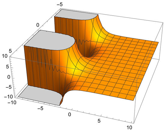
Figure 1. The solution$\mathit{h}\left(\mathit{x},\mathit{t}\right)$ of Example 1.

Example 2. 

Let us consider the heat equation given by:

$$h_t\left(x,t\right)=4h_{xx}\left(x,t\right), x,t\ge 0,$$

(36)

with the initial condition:$h\left(x,0\right)=\cos x ,$and the boundary conditions:$h\left(0,t\right)=e^{-4t},h_x\left(0,t\right)=0.$

Applying the FT to all conditions, we have:

$$A=\frac{v^2}{v^2+r^2} , B_1=\frac{s}{s+4u} , B_2=0 .$$

(37)

Applying DFT to Equation (36) and substituting all values of the transformed conditions in Equation (36), we have:

$$\begin{gathered} \left[\frac{s}{u}-\frac{4v^2}{r^2}\right]{ℛ}^2\left[h\left(x, t\right)\right]=\frac{s}{u}\left(\frac{v^2}{v^2+r^2}\right)-\frac{4v^2}{r^2}\left(\frac{s}{s+4u}\right) \\ =\frac{s{v}^2\left(s{r}^2-4v^{2}u\right)}{u{r}^2\left(v^2+r^2\right)\left(s+4u\right)}. \end{gathered}$$

Thus, one can get

$${ℛ}^2\left[h\left(x, t\right)\right]=\frac{s{v}^2\left(s{r}^2-4u{v}^2\right)}{u{r}^2\left(v^2+r^2\right)\left(s+4u\right)} \frac{u{r}^2}{\left(s{r}^2-4u{v}^2\right)}=\frac{s{v}^2}{\left(v^2+r^2\right)\left(s+4u\right)}.$$

(38)

Running the inverse DFT to Equation (38), then the solution of Equation (36) is

$$h\left(x, t\right)={{ℛ}^2}^{-1}\left[\frac{s}{s+4u} \frac{v^2}{v^2+r^2}\right]=e^{-4t}\cos x.$$

In the following, we present Figure 2 that presents the graph of the 3D exact solution of Example 2.

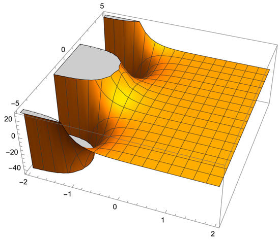
Figure 2. The solution$\mathit{h}\left(\mathit{x},\mathit{t}\right)$ of Example 2.

Example 3. 

Let us consider the heat equation given by

$$h_t\left(x,t\right)=h_{xx}\left(x,t\right)-2h\left(x,t\right), x,t\ge 0,$$

(39)

with the initial condition:$h\left(x,0\right)=\sinh x,$and the boundary conditions:$h\left(0,t\right)=0, h_x\left(0,t\right)=e^{-t}.$

Applying the formable transform to all conditions, we have

$$A=\frac{vr}{v^2-r^2} , B_1=0 , B_2=\frac{s}{s+u} .$$

(40)

Applying DFT to Equation (39) and substituting the values in Equation (32), we have

$$\left[\frac{s}{u}-\frac{v^2}{r^2}+2\right]{ℛ}^2\left[h\left(x, t\right)\right]=\frac{s}{u}\left(\frac{vr}{v^2-r^2}\right)-\frac{v}{r}\left(\frac{s}{s+u}\right)=\frac{sv\left(s{r}^2-v^{2}u+2u{r}^2\right)}{ur\left(v^2-r^2\right)\left(s+u\right)}.$$

Thus, after simple calculations, we get

$${ℛ}^2\left[h\left(x, t\right)\right]=\frac{svr}{\left(v^2-r^2\right)\left(s+u\right)}$$

(41)

Applying the inverse DFT to Equation (41), then the solution of Equation (39) is given by

$$h\left(x, t\right)={ℛ}^2{}^{-1}\left[\frac{s}{s+u} \frac{vr}{v^2-r^2}\right]=e^{-t}\sinh x.$$

In the following, we present Figure 3, that presents the graph of the 3D exact solution of Example 3.

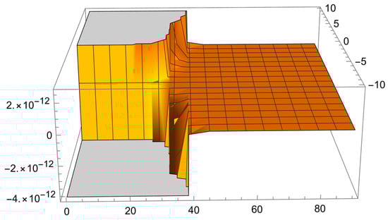
Figure 3. The solution$\mathit{h}\left(\mathit{x},\mathit{t}\right)$ of Example 3.

Example 4. 

Let us consider the heat equation given as:

$$h_t\left(x,t\right)=h_{xx}\left(x,t\right)+\sin x, x,t\ge 0,$$

(42)

with the initial condition:$h\left(x,0\right)=\cos x,$and the boundary conditions:$h\left(0,t\right)=e^{-t},h_x\left(0,t\right)=1-e^{-t}.$

Applying the formable transform to all the conditions, we have

$$A=\frac{v^2}{v^2+r^2} , B_1=\frac{s}{s+u} , B_2=1-\frac{s}{s+u}$$

(43)

Applying DFT to the Equation (42) and substituting the all the transformed values in Equation (43), we get

$$\begin{gathered} \left[\frac{s}{u}-\frac{v^2}{r^2}\right]{ℛ}^2\left[h\left(x, t\right)\right]=\frac{s}{u}\left(\frac{v^2}{v^2+r^2}\right)-\frac{v^2}{r^2}\left(\frac{s}{s+u}\right)-\frac{v}{r}\left(1-\frac{s}{s+u}\right)+\frac{vr}{v^2+r^2} \\ =\left[\frac{s{v}^2\left(s{r}^2-u{v}^2\right)}{u{r}^2\left(s+u\right)\left(v^2+r^2\right)}\right]+\left[\frac{v\left(s{r}^2-u{v}^2\right)}{r\left(s+u\right)\left(v^2+r^2\right)}\right]. \end{gathered}$$

Thus, after simple calculations, one can obtain

$${ℛ}^2\left[h\left(x, t\right)\right]=\left[\frac{s}{s+u} \frac{v^2}{v^2+r^2}\right]+\left[\frac{u}{s+u} \frac{vr}{v^2+r^2}\right]=\left[\frac{s}{s+u}\frac{v^2}{v^2+r^2}\right]+\left[\frac{s+u-s}{s+u} \frac{vr}{ v^2+r^2}\right].$$

(44)

Applying the inverse DFT to Equation (44), then the solution of Equation (42) is given by

$$h\left(x, t\right)={{ℛ}^2}^{-1}\left[\frac{s}{s+u}·\frac{v^2}{v^2+r^2}+\left(1-\frac{s}{s+u}\right)\frac{vr}{v^2+r^2}\right]=e^{-t}\cos x+\left(1-e^{-t}\right)\sin x.$$

In the following, we present Figure 4 that presents the graph of the 3D exact solution of Example 4.

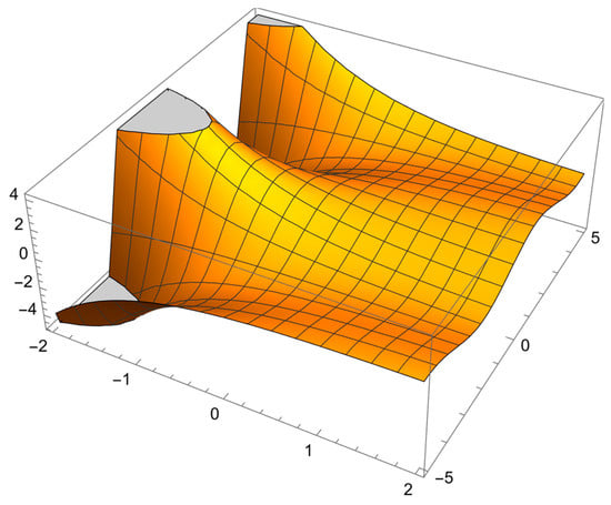
Figure 4. The solution$\mathit{h}\left(\mathit{x},\mathit{t}\right)$ of Example 4.

Example 5. 

Let us consider the heat equation given as

$$h_{xx}\left(x,t\right)-h_t\left(x,t\right)-3h\left(x,t\right)=-3, x,t\ge 0,$$

(45)

with the initial condition:$h\left(x,0\right)=1+\sin x,$and the boundary conditions:$h\left(0,t\right)=1 ,h_x\left(0,t\right)=e^{-4t}.$

Applying the formable transform to all conditions, we get

$$A=1+\frac{vr}{v^2+r^2} , B_1=1 , B_2=\frac{s}{s+4u} .$$

(46)

Applying the DFT to Equation (45) and substituting the all the values in Equation (46), we have

$$\begin{gathered} \left[\frac{s}{u}-\frac{v^2}{r^2}+3\right]{ℛ}^2\left[h\left(x, t\right)\right]=\frac{s}{u}\left(1+\frac{vr}{v^2+r^2}\right)-\frac{v^2}{r^2}-\frac{v}{r}\left(\frac{s}{s+4u}\right)+3 \\ =\left[\frac{s^2{r}^2-u{v}^2+3u{r}^2}{u{r}^2}\right]+svr\left[\frac{s{r}^2+4u{r}^2-u{v}^2-u{r}^2}{u{r}^2\left(s+4u\right)\left(v^2+r^2\right)}\right]. \end{gathered}$$

Thus, after simple computations, we have

$${ℛ}^2\left[h\left(x, t\right)\right]=1+\frac{svr}{\left(v^2+r^2\right)\left(s+4u\right)}$$

(47)

Applying the inverse DFT to Equation (47), then the solution of Equation (45) is

$$h\left(x, t\right)={{ℛ}^2}^{-1}\left[1+\frac{s}{s+4u}\frac{vr}{v^2+r^2}\right]=1+e^{-4t}\sin x.$$

In the following, we present Figure 5 that presents the graph of the 3D exact solution of Example 5.

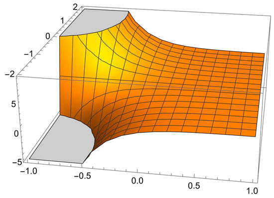
Figure 5. The solution$\mathit{h}\left(\mathit{x},\mathit{t}\right)$ of Example 5.

6. Conclusions

In this paper, we introduced a new double transform called the double formable transform. Several properties and theorems of the double transform were presented and proved. New results related to partial derivatives and the double convolution theorem were discussed and proved. Finally, we applied DFT to solve some applications on heat equations. A simple formula for solving heat partial differential equations were established, and used to solve some examples. The outcomes of this study show the strength and simplicity of DFT in solving partial differential equations. As a result, we intend to use it for solving more applications in the future, due to the simplicity and the advantage of preserving the constants values under the transform which reduces the calculations, in comparison to other integral transforms.

References

- El-Ajou, A.; Abu Arqub, O.; Momani, S. Homotopy analysis method for second-order boundary value problems of integrodifferential equations. Discret. Dyn. Nat. Soc. 2012, 2012, 365792. [Google Scholar] [CrossRef]
- Saadeh, A.; Qazza, K.; Amawi, A. New Approach Using Integral Transform to Solve Cancer Models. Fractal Fract. 2022, 6, 490. [Google Scholar] [CrossRef]
- Powers, D.L. Boundary Value Problems; Elsevier: Amsterdam, The Netherlands, 2014. [Google Scholar]
- Burqan, A.; Saadeh, R.; Qazza, A.; Momani, S. ARA-residual power series method for solving partial fractional differential equations. Alex. Eng. J. 2022, 62, 47–62. [Google Scholar] [CrossRef]
- Griffiths, D.F.; Higham, D.J. Numerical Methods for Ordinary Differential Equations: Initial Value Problems; Springer: London, UK, 2010. [Google Scholar]
- Al-Smadi, M.; Abu Arqub, O.; El-Ajou, A. A numerical iterative method for solving systems of first-order periodic boundary value problems. J. Appl. Math. 2014, 2014, 135465. [Google Scholar] [CrossRef]
- Hasan, S.; Al-Smadi, M.; El-Ajou, A.; Momani, S.; Hadid, S.; Al-Zhour, Z. Numerical approach in the Hilbert space to solve a fuzzy Atangana-Baleanu fractional hybrid system. Chaos Solitons Fractals 2021, 143, 110506. [Google Scholar] [CrossRef]
- Moa’ath, N.O.; El-Ajou, A.; Al-Zhour, Z.; Alkhasawneh, R.; Alrabaiah, H. Series solutions for nonlinear time-fractional Schrödinger equations: Comparisons between conformable and Caputo derivatives. Alex. Eng. J. 2020, 59, 2101–2114. [Google Scholar]
- El-Ajou, A.; Moa’ath, N.O.; Al-Zhour, Z.; Momani, S. Analytical numerical solutions of the fractional multi-pantograph system: Two attractive methods and comparisons. Results Phys. 2019, 14, 102500. [Google Scholar] [CrossRef]
- Saadeh, R.; Burqan, A.; El-Ajou, A. Reliable solutions to fractional Lane-Emden equations via Laplace transform and residual error function. Alex. Eng. J. 2022, 61, 10551–10562. [Google Scholar] [CrossRef]
- Ahmed, S.A.; Qazza, A.; Saadeh, R. Exact Solutions of Nonlinear Partial Differential Equations via the New Double Integral Transform Combined with Iterative Method. Axioms 2022, 11, 247. [Google Scholar] [CrossRef]
- Harjunkoski, I.; Maravelias, C.T.; Bongers, P.; Castro, P.M.; Engell, S.; Grossmann, I.E.; Hooker, J.; Méndez, C.; Sand, G.; Wassick, J. Scope for industrial applications of production scheduling models and solution methods. Comput. Chem. Eng. 2014, 62, 161–193. [Google Scholar] [CrossRef]
- Karbalaie, A.; Muhammed, H.H.; Shabani, M.; Montazeri, M.M. Exact Solution of Partial Differential Equation Using Homo-Separation of Variables. Int. J. Nonlinear Sci. 2014, 17, 84–90. [Google Scholar]
- Larsson, S.; Thomée, V. Partial Differential Equations with Numerical Methods; Springer: Berlin/Heidelberg, Germany, 2003. [Google Scholar]
- Saadeh, R.; Al-Smadi, M.; Gumah, G.; Khalil, H.; Khan, R.A. Numerical investigation for solving two-point fuzzy boundary value problems by reproducing kernel approach. Appl. Math. Inf. Sci. 2016, 10, 2117–2129. [Google Scholar] [CrossRef]
- You, Y.L.; Kaveh, M. Fourth-order partial differential equations for noise removal. IEEE Trans. Image Process. 2000, 9, 1723–1730. [Google Scholar] [CrossRef] [PubMed]
- Qazza, A.; Burqan, A.; Saadeh, R.; Khalil, R. Applications on Double ARA–Sumudu Transform in Solving Fractional Partial Differential Equations. Symmetry 2022, 14, 1817. [Google Scholar] [CrossRef]
- Ahmed, S.; Elzaki, T.; Elbadri, M.; Mohamed, M.Z. Solution of partial differential equations by new double integral transform (Laplace—Sumudu transform). Ain Shams Eng. J. 2021, 12, 4045–4049. [Google Scholar] [CrossRef]
- Saadeh, R.; Qazza, A.; Burqan, A. On the Double ARA-Sumudu Transform and Its Applications. Mathematics 2022, 10, 2581. [Google Scholar] [CrossRef]
- Ahmed, S.; Elzaki, T.; Hassan, A.A. Solution of integral differential equations by new double integral transform (Laplace-Sumudu transform). J. Abstr. Appl. Anal. 2020, 2020, 4725150. [Google Scholar] [CrossRef]
- Elnaqeeb, T.; Shah, N.A.; Vieru, D. Weber-Type Integral Transform Connected with Robin-Type Boundary Conditions. Mathematics 2020, 8, 1335. [Google Scholar] [CrossRef]
- Butzer, P.L.; Jansche, S. A direct approach to the Mellin transform. J. Fourier Anal. Appl. 1997, 3, 325–376. [Google Scholar] [CrossRef]
- Sullivan, D.M. Z-transform theory and the FDTD method. IEEE Trans. Antennas Propag. 1996, 44, 28–34. [Google Scholar] [CrossRef]
- Layman, J.W. The Hankel transform and some of its properties. J. Integer Seq. 2001, 4, 1–11. [Google Scholar]
- Chauhan, R.; Kumar, N.; Aggarwal, S. Dualities between Laplace-Carson transform and some useful integral transforms. Int. J. Innov. Technol. Explor. Eng. 2019, 8, 1654–1659. [Google Scholar] [CrossRef]
- Belgacem, F.B.; Karaballi, A.A. Sumudu transform fundamental properties investigations and applications. Int. J. Stoch. Anal. 2006, 2006, 091083. [Google Scholar] [CrossRef]
- Saadeh, R.; Ghazal, B. A new approach on transforms: Formable integral transform and its applications. Axioms 2021, 10, 332. [Google Scholar] [CrossRef]
Disclaimer/Publisher’s Note: The statements, opinions and data contained in all publications are solely those of the individual author(s) and contributor(s) and not of MDPI and/or the editor(s). MDPI and/or the editor(s) disclaim responsibility for any injury to people or property resulting from any ideas, methods, instructions or products referred to in the content. |
© 2023 by the authors. Licensee MDPI, Basel, Switzerland. This article is an open access article distributed under the terms and conditions of the Creative Commons Attribution (CC BY) license (https://creativecommons.org/licenses/by/4.0/).