
Optimal Design of a Canopy Using Parametric Structural Design and a Genetic Algorithm

 ,
,  , ,
, , 
Abstract
1. Introduction
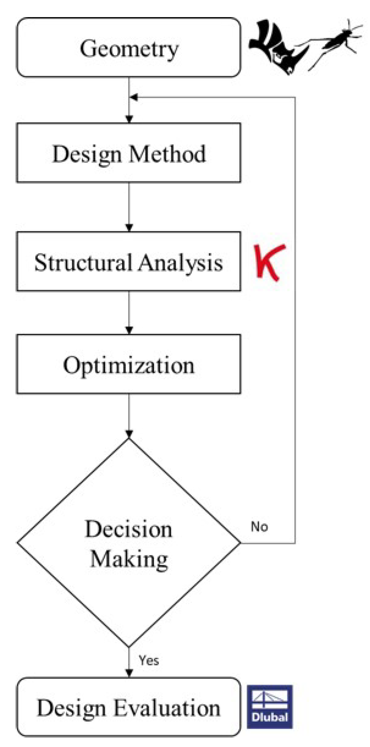
2. Method
2.1. Structural Optimization
2.2. Genetic Algorithm
- Fitness function.
- Selection.
- Mechanism.
- Coalescence Algorithm.
- Mutation factory.
2.3. Dynamic Relaxation
- Anchor: This maintains a point’s original position, and it is used to hold the mesh’s corners in place.
- Length (Line): This goal object aims to maintain two points (line endpoints) at a specific length apart. The points move less when the strength is increased.
- Load: This goal object applies a normal force on the points. The force is specified as a vector, and the length of the vector is proportional to the magnitude of the applied load.
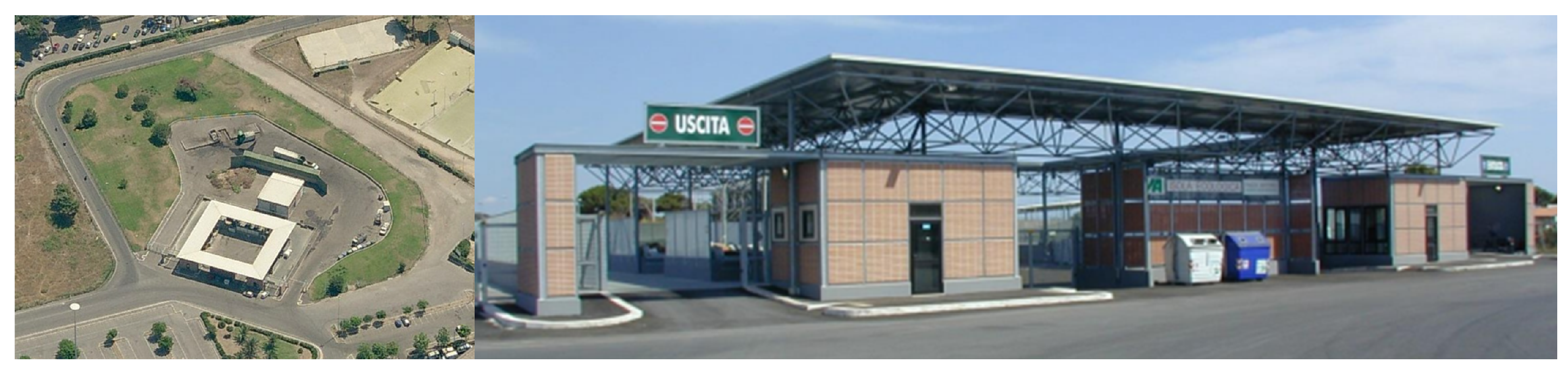
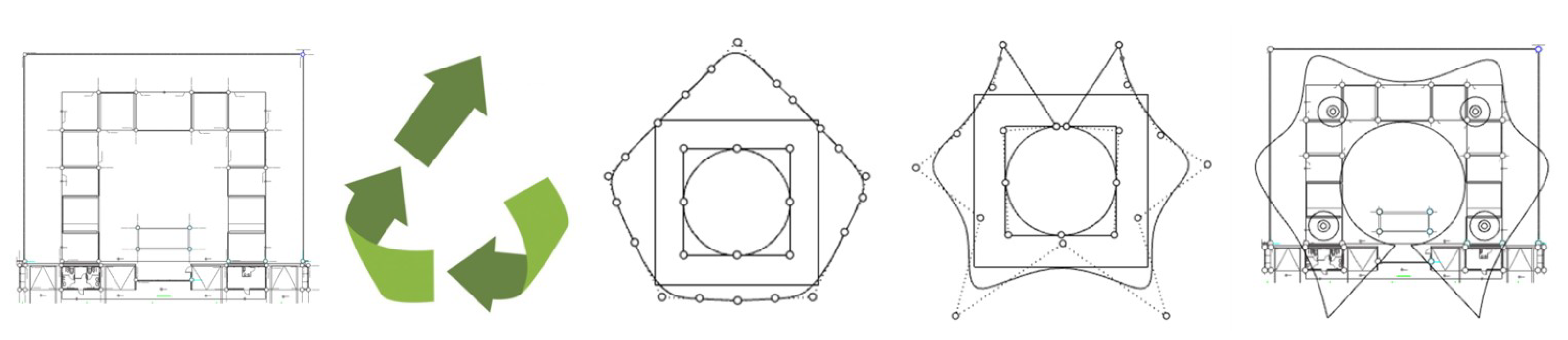
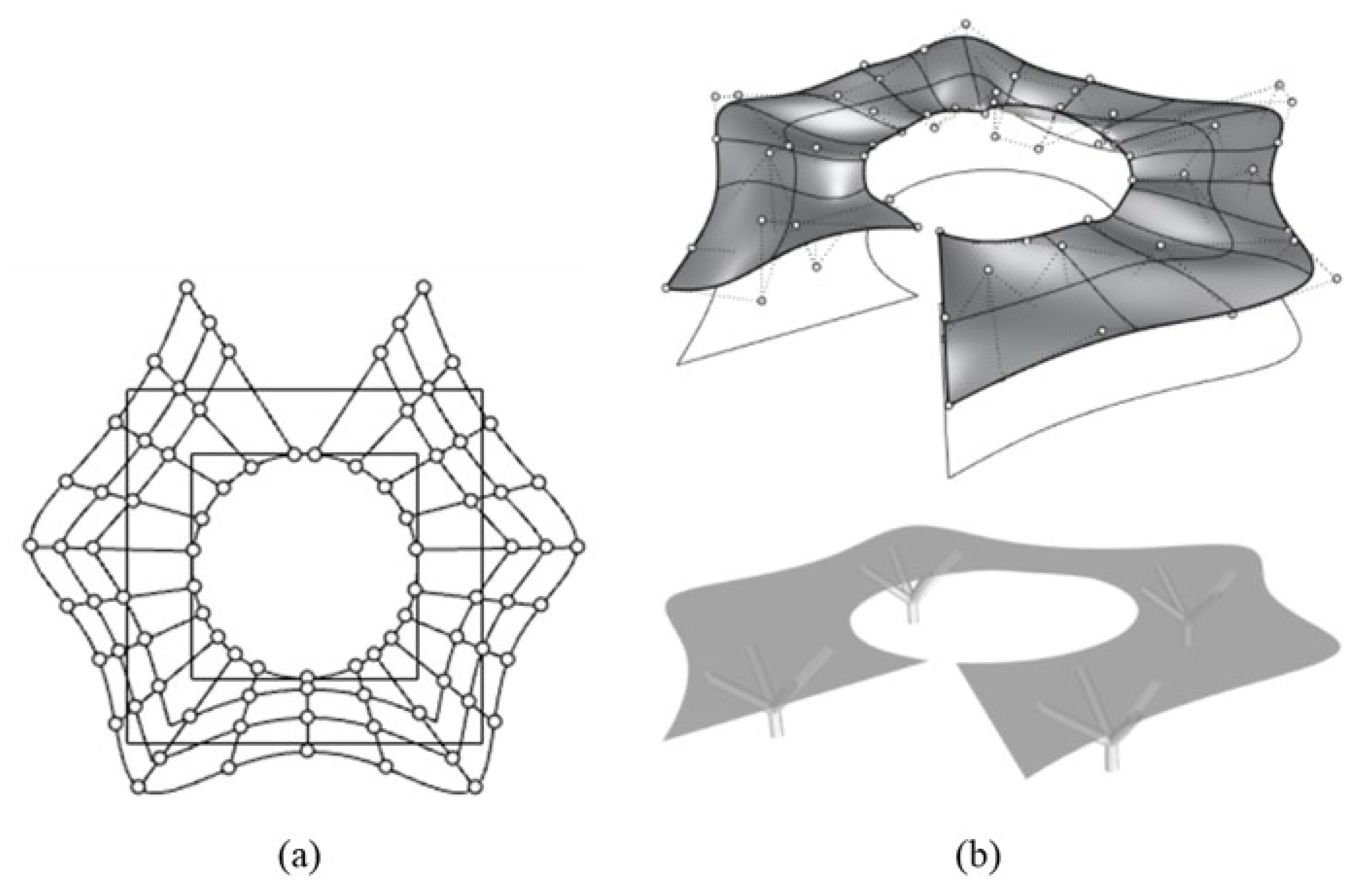
3. Application
4. Results
5. Conclusions
Author Contributions
Funding
Data Availability Statement
Conflicts of Interest
References
- Mei, L.; Wang, Q. Structural Optimization in Civil Engineering: A Literature Review. Buildings 2021, 11, 66. [Google Scholar] [CrossRef]
- Bletzinger, K.U.; Wüchner, R.; Daoud, F.; Camprubí, N. Computational methods for form finding and optimization of shells and membranes. Comput. Methods Appl. Mech. Eng. 2005, 194, 3438–3452. [Google Scholar] [CrossRef]
- Md Rian, I.; Sassone, M. Tree-inspired dendriforms and fractal-like branching structures in architecture: A brief historical overview. Front. Archit. Res. 2014, 3, 298–323. [Google Scholar] [CrossRef]
- Veenendaal, D.; Augustynowicz, E.; Tang, G. Magnolia: A glass-fibre reinforced polymer gridshell with a novel pattern and deployment concept. In Proceedings of the IASS Annual Symposia, Hamburg, Germany, 25–28 September 2017. [Google Scholar]
- Vierlinger, R.; Hofmann, A.; Bollinger, K. Emergent Hybrid Prefab Structures in Dwellings. In Proceedings of the IASS Annual Symposia, Washington, DC, USA, 29–31 October 2013. [Google Scholar] [CrossRef]
- Pugnale, A. Engineering Architecture Advances of a Technological Practice. Ph.D. Thesis, Politecnico di Torino, Torino, Italy, 2009. [Google Scholar]
- Ali, K. Computational Structural Analysis and Finite Element Methods, 1st ed.; Springer: Cham, Switzerland, 2014. [Google Scholar] [CrossRef]
- Kaveh, A.; Rahami, H.; Shojaei, I. Swift Analysis of Structures Using Graph Theory Methods; Springer: Berlin/Heidelberg, Germany, 2020. [Google Scholar]
- Ali, K. Optimal Analysis of Structures by Concepts of Symmetry and Regularity, 1st ed.; Springer: Vienna, Austria, 2013. [Google Scholar] [CrossRef]
- Ali, K. Topological Transformations for Efficient Structural Analysis, 1st ed.; Springer: Cham, Switzerland, 2022. [Google Scholar] [CrossRef]
- Kirsch, U. Optimum Structural Design; McGraw-Hill: New York, NY, USA, 1981. [Google Scholar]
- Ali, K. Advances in Metaheuristic Algorithms for Optimal Design of Structures, 3rd ed.; Springer: Berlin/Heidelberg, Germany, 2021. [Google Scholar] [CrossRef]
- Kaveh, A.; Bakhshpoori, T. Metaheuristics: Outlines, MATLAB Codes and Examples; Springer: Berlin/Heidelberg, Germany, 2019. [Google Scholar] [CrossRef]
- Trovalusci, P.; Panei, R.; Tinelli, A. Computational optimization in architectural design and constructive issues. A case study: The canopy of a waste collection center. In Structures and Architecture: Bridging the Gap and Crossing Borders; Taylor and Francis Group: Abingdon, UK, 2019; pp. 1072–1079. [Google Scholar] [CrossRef]
- Panei, R.; Trovalusci, P.; Tinelli, A. The “question of the technique”: From the designing idea to the realized form: Beyond their Limits. In Structures and Architecture; Taylor and Francis Group: Abingdon, UK, 2016; pp. 519–526. [Google Scholar] [CrossRef]
- Benvenuto, E. An Introduction to the History of Structural Mechanics, 3rd ed.; Springer: New York, NY, USA, 1991. [Google Scholar]
- Pottmann, H.; Eigensatz, M.; Vaxman, A.; Wallner, J. Architectural Geometry. Comput. Graph. 2015, 47, 145–164. [Google Scholar] [CrossRef]
- Rutten, D. Galapagos: On the Logic and Limitations of Generic Solvers. Archit. Des. 2013, 83, 132–135. [Google Scholar] [CrossRef]
- Naboni, R. Architectural Morphogenesis Through Topology Optimization. In Handbook of Research on Form and Morphogenesis in Modern Architectural Contexts; IGI Global: Hershey, PA, USA, 2018; Chapter 4; pp. 69–92. [Google Scholar] [CrossRef][Green Version]
- Mueller, C.; Ochsendorf, J. An Integrated Computational Approach for Creative Conceptual Structural Design. In Proceedings of the IASS Annual Symposia, Washington, DC, USA, 29–31 October 2013; pp. 1–6. [Google Scholar]
- Danhaive, R.; Mueller, C.T. Design subspace learning: Structural design space exploration using performance-conditioned generative modeling. Autom. Constr. 2021, 127, 103664. [Google Scholar] [CrossRef]
- Mizobuti, V.; Vieira Junior, L.C. Bioinspired architectural design based on structural topology optimization. Front. Archit. Res. 2020, 9, 264–276. [Google Scholar] [CrossRef]
- Wortmann, T.; Tunçer, B. Differentiating parametric design: Digital workflows in contemporary architecture and construction. Des. Stud. 2017, 52, 173–197. [Google Scholar] [CrossRef]
- Tedeschi, A.; Andreani, S. AAD, Algorithms-Aided Design: Parametric Strategies Using Grasshopper; Le Penseur Publisher: Brienza, Italy, 2014. [Google Scholar]
- Ohmori, H. Computational Morphogenesis: Its Current State and Possibility for the Future. Int. J. Space Struct. 2011, 26, 269–276. [Google Scholar] [CrossRef]
- Akbarzadeh, M.; Van Mele, T.; Block, P. On the equilibrium of funicular polyhedral frames and convex polyhedral force diagrams. Comput.-Aided Des. 2015, 63, 118–128. [Google Scholar] [CrossRef]
- Trovalusci, P.; Panei, R. Towards an ethic of construction: The structural conception and the influence of mathematical language in architectural design. In Proceedings of the Tectonics in Architecture, between Aesthetics and Ethics, ICSA 2010, Guimaraes, Portugal, 24–26 July 2010. [Google Scholar]
- Piker, D. Kangaroo: Form Finding with Computational Physics. Archit. Des. 2013, 83, 136–137. [Google Scholar] [CrossRef]
- Rutten, D. Evolutionary Principles Applied to Problem Solving. Grasshopper Algorithmic Modeling for Rhino. Available online: https://www.grasshopper3d.com/profiles/blogs/evolutionary-principles (accessed on 26 September 2021).
- Preisinger, C. Linking Structure and Parametric Geometry. Archit. Des. 2013, 83, 110–113. [Google Scholar] [CrossRef]
- Muhsen, H.; Al-Kouz, W.; Khan, W. Small Wind Turbine Blade Design and Optimization. Symmetry 2020, 12, 18. [Google Scholar] [CrossRef]
- Ni, P.; Gao, J.; Song, Y.; Quan, W.; Xing, Q. A New Method for Dynamic Multi-Objective Optimization Based on Segment and Cloud Prediction. Symmetry 2020, 12, 465. [Google Scholar] [CrossRef]
- Christiansen, A.N.; Bærentzen, J.A.; Nobel-Jørgensen, M.; Aage, N.; Sigmund, O. Combined shape and topology optimization of 3D structures. Comput. Graph. 2015, 46, 25–35. [Google Scholar] [CrossRef]
- Wu, Z.; Xiao, R. Substructure-Based Topology Optimization for Symmetric Hierarchical Lattice Structures. Symmetry 2020, 12, 678. [Google Scholar] [CrossRef]
- Wang, Q.; Wang, X.; Luo, H.; Xiong, J. An Improved Multi-Objective Evolutionary Approach for Aerospace Shell Production Scheduling Problem. Symmetry 2020, 12, 509. [Google Scholar] [CrossRef]
- Veenendaal, D.; Bakker, J.; Block, P. Structural Design of the Flexibly Formed, Mesh-Reinforced Concrete Sandwich Shell Roof of NEST HiLo. J. Int. Assoc. Shell Spat. Struct. 2017, 58, 23–38. [Google Scholar] [CrossRef]
- Goldberg, D. Genetic Algorithms in Search, Optimization and Machine Learning, 1st ed.; Addison Wesley Professional: Boston, MA, USA, 1989. [Google Scholar]
- Cubukcuoglu, C.; Ekici, B.; Tasgetiren, M.F.; Sariyildiz, S. OPTIMUS: Self-Adaptive Differential Evolution with Ensemble of Mutation Strategies for Grasshopper Algorithmic Modeling. Algorithms 2019, 12, 141. [Google Scholar] [CrossRef]
- Storn, R.; Price, K. Differential Evolution—A Simple and Efficient Heuristic for global Optimization over Continuous Spaces. J. Glob. Optim. 1997, 11, 341–359. [Google Scholar] [CrossRef]
- Wortmann, T. Genetic evolution vs. function approximation: Benchmarking algorithms for architectural design optimization. J. Comput. Des. Eng. 2018, 6, 414–428. [Google Scholar] [CrossRef]
- Sigrid, A.; Philippe, B.; Veenendaal, D.; Williams, C. Shell Structures for Architecture: Form Finding and Optimization; Routledge: London, UK, 2014. [Google Scholar] [CrossRef]
- Barnes, M.R. Form Finding and Analysis of Tension Structures by Dynamic Relaxation. Int. J. Space Struct. 1999, 14, 89–104. [Google Scholar] [CrossRef]
- Seiichi, S. Topology-Driven Form-Finding: Interactive Computational Modelling of Bending-active and Textile Hybrid Structures through Active-Topology Based Real-Time Physics Simulations, and Its Emerging Design Potentials. Ph.D. Thesis, University of Stuttgart, Stuttgart, Germany, 2020. [Google Scholar]
- Panei, R.; Petrucciani, G.; Bonanni, D.; Trovalusci, P. ECOSITING: A Sit Platform for Planning the Integrated Cycle of Urban Waste. In International Symposium on New Metropolitan Perspectives; Calabr, F., Della Spina, L., Bevilacqua, C., Eds.; Springer: Cham, Switzerland, 2019; pp. 585–592. [Google Scholar] [CrossRef]
- Bozza, A.; Asprone, D.; Fabbrocino, F. Urban Resilience: A Civil Engineering Perspective. Sustainability 2017, 9, 103. [Google Scholar] [CrossRef]
- Mohammadzadeh Gheshlaghi, R.; Akbulut, H. Modeling and Analysis of Anisogrid Lattice Structures Using an Integrated Algorithmic Modelling Framework. Comput. Res. Prog. Appl. Sci. Eng. (CRPASE) Trans. Mech. Eng. 2020, 6, 6–10. [Google Scholar]
- Morozov, E.; Lopatin, A.; Nesterov, V. Finite-element modelling and buckling analysis of anisogrid composite lattice cylindrical shells. Compos. Struct. 2011, 93, 308–323. [Google Scholar] [CrossRef]


Disclaimer/Publisher’s Note: The statements, opinions and data contained in all publications are solely those of the individual author(s) and contributor(s) and not of MDPI and/or the editor(s). MDPI and/or the editor(s) disclaim responsibility for any injury to people or property resulting from any ideas, methods, instructions or products referred to in the content. |
© 2023 by the authors. Licensee MDPI, Basel, Switzerland. This article is an open access article distributed under the terms and conditions of the Creative Commons Attribution (CC BY) license (https://creativecommons.org/licenses/by/4.0/).
Share and Cite
Dasari, S.K.; Fantuzzi, N.; Trovalusci, P.; Panei, R.; Pingaro, M. Optimal Design of a Canopy Using Parametric Structural Design and a Genetic Algorithm. Symmetry 2023, 15, 142. https://doi.org/10.3390/sym15010142
Dasari SK, Fantuzzi N, Trovalusci P, Panei R, Pingaro M. Optimal Design of a Canopy Using Parametric Structural Design and a Genetic Algorithm. Symmetry. 2023; 15(1):142. https://doi.org/10.3390/sym15010142
Chicago/Turabian StyleDasari, Saaranya Kumar, Nicholas Fantuzzi, Patrizia Trovalusci, Roberto Panei, and Marco Pingaro. 2023. "Optimal Design of a Canopy Using Parametric Structural Design and a Genetic Algorithm" Symmetry 15, no. 1: 142. https://doi.org/10.3390/sym15010142
APA StyleDasari, S. K., Fantuzzi, N., Trovalusci, P., Panei, R., & Pingaro, M. (2023). Optimal Design of a Canopy Using Parametric Structural Design and a Genetic Algorithm. Symmetry, 15(1), 142. https://doi.org/10.3390/sym15010142