Article

A Genetic Algorithm for the Waitable Time-Varying Multi-Depot Green Vehicle Routing Problem

1
College of Computer Science and Engineering, Shandong University of Science and Technology, Qingdao 266590, China
2
Qingdao GraceChain Software Ltd., Qingdao 266100, China
*
Author to whom correspondence should be addressed.
Symmetry 2023, 15(1), 124; https://doi.org/10.3390/sym15010124
Submission received: 17 October 2022 / Revised: 12 December 2022 / Accepted: 16 December 2022 / Published: 1 January 2023

Abstract

:
In an era where people in the world are concerned about environmental issues, companies must reduce distribution costs while minimizing the pollution generated during the distribution process. For today’s multi-depot problem, a mixed-integer programming model is proposed in this paper to minimize all costs incurred in the entire transportation process, considering the impact of time-varying speed, loading, and waiting time on costs. Time is directional; hence, the problems considered in this study are modeled based on asymmetry, making the problem-solving more complex. This paper proposes a genetic algorithm combined with simulated annealing to solve this issue, with the inner and outer layers solving for the optimal waiting time and path planning problem, respectively. The mutation operator is replaced in the outer layer by a neighbor search approach using a solution acceptance mechanism similar to simulated annealing to avoid a local optimum solution. This study extends the path distribution problem (vehicle-routing problem) and provides an alternative approach for solving time-varying networks.

1. Introduction

With increasing global concerns about environmental issues, the greenhouse effect is gaining more attention. Greenhouse gases are one of the causes of the greenhouse effect. According to the United Nations Framework Convention on Climate Change—UNFCCC (1997) Kyoto protocol, definite measures have to be taken to curb carbon emissions [1]. The transportation sector is the largest contributor to global carbon emissions [2]. Therefore, one effective method to improve the greenhouse effect is to control carbon dioxide emissions produced during the distribution process. Carbon dioxide emissions and fuel consumption are positively correlated to some extent, and fuel consumption depends on vehicle type, traffic conditions, and environmental conditions. Many companies are exploring methods to account for environmental pollution from transportation based on lower fuel costs. For example, Walmart, General Mills, and Anheuser-Busch are all exploring methods to reduce fuel consumption in their transportation fleets [3,4,5]. Reducing the energy consumption of vehicles is a crucial issue in the logistics distribution process [6,7,8]. Thus, research aimed at reducing fuel consumption in the distribution process, namely, the green path problem, has been conducted.
Existing models for calculating vehicle energy consumption for the green path problem fall into two types, one only considers the fixed condition of the vehicle itself but does not consider the speed [9]. However, the actual road conditions will change at any time, so the fuel consumption of cars is unstable. Therefore, some studies have suggested that changes in vehicle speed due to road conditions should be considered when calculating vehicle fuel consumption [10,11]. Bektas [12] used an integrated emission model to calculate fuel consumption and pollution emissions, considering speed as a factor for the first time. Most existing studies assume that cars travel at a constant speed, largely ignoring the effects of congestion, especially in urban areas. Therefore, Kuo et al. [13] made the first attempt to include the time-varying speed, that is, a speed that varies continuously with time, in the consideration of the path problem, and applied Taboo Search to solve the VRP for the objective function related to fuel consumption. Most existing studies on time-varying processes are mainly based on two types of speed representations: piecewise constant function [14] and piecewise continuous function [15]. The Federal Highway Administration highlights that speed does not change at a single moment, but rather smoothly. Therefore, the method of expressing vehicle speed as a piecewise continuous function is more realistic.
Simultaneously, a new model of “multi-depot collaboration” has been naturally formed to improve efficiency and make goods reach customers in time due to the boom in e-commerce. “Multi-depot cooperation” means that goods are shared between each depot, and vehicles are also shared between depots so that vehicles can leave from any depot and return to any other depot. The application of “multi-depot collaboration” in the distribution process has drastically improved efficiency, effectively integrated resources [16], and reduced labor and transportation costs. Thus, the new model of “multi-depot collaboration” has become the primary choice of many companies. Here, we take Figure 1 as an example to introduce the specific distribution process under the environment of “multi-depot collaboration,” in which there are four depots and five customers, which are served by two vehicles. The vehicles can be driven from any depot and finally returned to any depot because the resources owned by the four depots are openly shared in the distribution process, and the resources needed by the customers are available in each depot in sufficient quantity. Taking vehicle 1 as an example, vehicle 1 loads goods in depot 1, departs to start distribution, passes through customers 1 and 2, and, finally, returns to depot 2.
The customer’s receipt time is usually a soft time window in a natural multi-depot environment. For this problem, this study considers dividing the cost into the time window cost, fixed cost, and fuel consumption cost. Clearly, the speed is different at different times, and when a vehicle is found to be congested at a customer’s point of delivery, perhaps waiting at that customer’s point until the road conditions are suitable before departing will effectively reduce the fuel consumption cost of transportation. In Figure 1, for each customer node, in addition to the unloading area, an additional waitable area is set up, assuming that vehicle 1 is serving customer 2. When it is found that the road conditions become congested, the vehicle chooses to wait in the waitable area at customer 2 after the service is completed, up to the moment when the road conditions are better or conducive to reducing fuel consumption costs before departing for depot 2.
Therefore, the cost is divided into time-window cost, fixed cost, and fuel-consumption cost in an environment with time-varying speed and multi-depot coordination. The goal is to minimize the total cost of the three costs accumulated, use fewer vehicles, consume less fuel, and meet the time-window requirements of most customers. Furthermore, calculating whether to wait and how long to wait for the lowest cost is important. The proposed time-varying multi-depot green vehicle routing problem with an elective waiting policy is a green path extension problem. It considers resting on the node to wait for a better departure time in a time-varying case.
Arijit proposed a hybrid particle swarm optimization algorithm with a basic variable neighborhood search algorithm to solve carbon emissions in the field of marine transportation [17]. Inspired by this, this study proposes a hybrid dual-layer genetic algorithm based on variable neighborhood searches. The time distance between two points is closely related to the selection of the starting point because of the directivity of time and asymmetry of the graph. The outer layer of the algorithm generates an initial population after grouping customers according to their spatio-temporal distances. It then iteratively optimizes them using an adaptive neighborhood search strategy and an adaptive genetic algorithm. The inner layer of the algorithm uses an adaptive genetic algorithm to obtain a better path and the waiting time of the corresponding path under the elective waiting strategy. The experimental results show that the multi depot green path obtained under the elective waiting strategy can effectively reduce the cost in the transportation process.
The contributions of this paper are as follows:
  • Considering that the real road conditions are always changing, a waiting mechanism is introduced to allow vehicles to wait at some nodes to optimize the vehicle path.
  • A dual-layer genetic algorithm is developed to solve the proposed problem, and the advantages of neighborhood search and simulated annealing are introduced to make the algorithm more effective.
The remainder of this paper is organized as follows. Section 2 introduces related literature on several types of problems closely related to this study. Section 3 introduces the problems and mathematical models proposed in this study. Section 4 introduces the algorithms and the components proposed in this study. Section 5 presents the experimental results. Finally, Section 6 presents a summary of our study and future research ideas.

2. Related Work

The problem studied in this paper is the extension of the green path problem, considering reality and finding a better planning result. This article reviews three types of issues: the time-dependent vehicle-routing problem (TDVRP), multi-depot vehicle-routing problem (MDVRP), and waiting vehicle-routing problem (WVRP).

2.1. Time-Dependent Vehicle Routing Problem, TDVRP

To the best of our knowledge, Beasley [18] was the first to consider time-varying and divided a day into several non-overlapping time slots, with different transmission times within each time slot. The solution was obtained using the savings algorithm proposed by Clarke and Wright [19]. One of the most significant drawbacks of using transmission time is that it does not fit the ‘FIFO’ strategy, that is, when two cars start from the same point, then the vehicle that starts later may even reach the end before the car that starts first, which is not in line with the reality. Subsequently, Hill [20] proposed a simple model of time-varying speed. The speed changed only between cycles, and the speed in each cycle was constant. Several methods for estimating the parameters of this model have also been presented. This approach also has some drawbacks: it is apparent that there will not be a constant state of speed in daily life because it is constantly changing with time. Horn [21] approximated the velocity in different periods using a function to represent a continuously varying velocity with a segmented linear function. Ichoua [14] discussed the model’s characteristics. Experiments were conducted to evaluate the model in static and dynamic environments. The experimental results show that the time-dependent velocity model exhibits a more significant improvement than the fixed velocity model. Jie [22] used piecewise continuous functions to simulate speed. A time-varying vehicle-routing problem with a soft time window was constructed. The goal of this problem is to minimize the total distribution cost. A hybrid algorithm, HA, is proposed to solve the problem by combining the scanning algorithm with the improved PSO algorithm. Ming [23] investigated the low-carbon vehicle path problem for cold chain logistics, considering time-varying traffic circumstances, and offered a low-carbon cold-chain logistics path optimization model that aimed to lower carbon emissions and distribution costs. The model was solved using an optimized non-dominated ranking genetic algorithm II (NSGA-II) engine to convert a Pareto frontal solution set.

2.2. Multi-Depot Vehicle Route Problem, MDVRP

Tillman [24] first proposed the multi-depot vehicle route problem (MDVRP) and solved it using a preservation algorithm. Wren and Holliday [25] successfully solved the MDVRP problem for 176 customer points in two depots using the Sweep Method. Raft et al. [26] used a two-stage clustering strategy before routing to address the MDVRP problem. Sadati [27] demonstrated a variable taboo neighborhood search (VTNS) mechanism for creating a class of multi-depot vehicle routing problems (MDVRP) that make use of taboo in a variable neighborhood. The forbade jitter mechanism is practiced during the search’s diversification phase. Furthermore, the approach allows for the violation of problem-specific restrictions during the search process to eliminate the local optimum and converge to a high-quality viable solution. Lim [28] proposed a new single-stage approach for solving MDVRP that differs from the two-stage approach commonly used internationally but solves the MDVRP problem effectively. Gulczynski, Golden, and Wasil [29] proposed a heuristic algorithm based on integer programming that aims to handle vehicles located in the same parking lot and vehicles located between the fact that orders can be delivered in batches to reduce the travel distance. Cornillier, Boctor, and Renaud [30] stated a MILP model for solving the multi-network issue for heterogeneous fleets to maximize operating income while considering maximum and minimum demand limitations. Allahyari [31] put forward a hybrid heuristic method to solve MDVRP that reflects the greedy randomized adaptive search, ILS, and SA multiple heuristics. Bezerra [32] outlined a technique for rebutting the multi-depot vehicle routing problem based on the generalized variable neighborhood search metaheuristic (MDVRP). The technique is evaluated in a classic example of this allegation and generates a random variable neighborhood descent as a local search framework. Brando [33] devised an iterative local model in which the actions performed during the local search were executed and, subsequently, used to describe the perturbation processes. The issue at hand is a multi-depot open vehicle path problem, which differs from the classic vehicle path problem in two ways: there are multiple depots. Thus, the vehicle does not return to the depot after delivering the goods to the customer; that is, the starting point is not at the end of the route.

2.3. Waiting Vehicle Routing Problem, WVRP

To the best of our knowledge, Halpern [34] was the first to propose the waiting shortest path problem. He discussed the issue of finding the shortest path between any two nodes in the graph, but the time-cost in a path might change at different moments. The proposed method is based on Dijkstra’s shortest path algorithm, optimized by postponing departure at a specific moment to resolve this problem. Subsequently, Orda [35] presented a technique for determining the shortest path with the least delay under various waiting limitations and analyzed the aspects of the resultant paths. The shortest-path problem is classified into three varieties by Cai [36]: arbitrary waiting, no waiting, and finite waiting. Then, several approaches are offered for answering the typical finite waiting problem. The general model of time-varying shortest paths considered by Cai [37] restricts waiting at the vertex with a waiting cost and accelerates on an arc with an acceleration cost. Dean [38] investigated the issue of the lowest cost in time-varying networks by waiting at particular nodes to lower the cost through the arc and discussed various elective waiting approaches. Lei [39] proposed the MORT problem, which exploits parking facilities in a road system and reduces road trip time. He, subsequently, developed an approximation method and two new algorithms to resolve this issue more swiftly. Omer [40] considered a time-varying network of shortest paths where waiting is empowered, the total waiting time is bounded for continuous and segmented linear arc travel time functions, and each waiting period at each node is bounded. The goal of this solution is to reduce the general travel time instead of the travel time to the destination. He [41] explored two different methods for shortest paths, the first of which allowed waiting at some nodes but at a cost. The second limitation is the total maximum waiting time.
In the above WVRP problems, most of them use time-varying transmission time to directly represent the transmission cost between two points. That is, the transmission time between two points is directly determined by the departure time, and some effective solutions to the waiting problem are proposed. However, this does not conform to FIFO characteristics because late departure vehicles may arrive at the destination earlier than early departure vehicles. In this paper, piecewise continuous function is used to express time-varying speed, so the algorithm conforms to the FIFO characteristics and is more practical. Most of the existing ones consider the waiting strategy on the shortest-path problem. This paper extends it to vehicle routing problem, and uses waiting strategy to reduce the total distribution cost.
The latest research of MDVRP is that Fan [42] proposed an integer programming model with the minimum total cost for the multi-depot vehicle routing problem under the time-varying road network, considering the fixed cost of vehicles, the penalty cost of advance and delay, the fuel cost, the impact of vehicle speed, as well as load and road slope on fuel consumption. Therefore, we add the elective waiting policy to the problem and extend it to obtain the MDVRP problem with the elective waiting policy proposed in this study.

3. Problem and Mathematical Model

3.1. Problem Definition

The multi-depot vehicle routing problem presented in this study is an extension of the vehicle routing problem. This study considers the multi-depot distribution path problem in a time-varying situation. Specifically, the path network can be described as a completely undirected graph in which the velocity on each edge continuously changes with time. All vehicles in the path network were of the same type and capacity. At some point, all vehicles leave the depot where they are located, visit the customers on the vehicle segment, and deliver goods to the customers according to their requirements for the time window; early arrival or late arrival is charged with a corresponding penalty. The vehicles return to any depot after completing the delivery service to all customers. Delivery costs consist of fixed costs, fuel consumption, and time window penalties and are affected by speed, load, etc. There is an optimal departure time for transportation between the two points to minimize the cost of transportation because the speed varies with time. This study investigates the multi-depot vehicle routing problem with time windows under an elective waiting policy. The parameters and definitions used in the text are shown in Table 1.
The problem proposed in this paper is how to solve the access sequence of each vehicle to the designated customer point. The output is also the access order of the corresponding vehicles; therefore, the variable is an integer. However, in the calculation process, the variable of the internal genetic algorithm is the waiting time, which is not an integer but a decimal value. Therefore, this paper proposes a mixed-integer model.

3.2. Fuel Consumption

Bektas [12] proposed a relationship function between fuel consumption F and CO2 emissions E, as expressed in Equation (1).
F = E μ 1 + μ 2
Therefore, the emissions of a section of a path can be obtained first to determine the fuel consumption, and then the fuel quantity is calculated.
The proposed method uses the MEET model proposed by Hickman [43] to calculate emissions. This model considered the effects of vehicle speed, road gradient, and vehicle load on CO2 emissions and is more in line with the real environment in realistic situations, as expressed in Equation (2).
e = ( 110 + 0.000375 v 3 + 8720 / v ) × L C × G C
In this equation, e is the emission generated per kilometer (g/km), v is the vehicle speed in km/h, and L C is the vehicle load correction factor, as expressed in Equation (3). The road gradient modification is referred to as G C , as expressed in Equation (4).
L C = 0.27 δ + 1 + 0.0614 ζ δ ζ 3 δ 0.00235 v δ ( 1.33 / v ) δ
G C = e x p ( ( 0.0059 v 2 0.775 v + 11.936 ) ζ )
In the above equation, ζ represents the road slope, where a percentage is used to represent the road slope, v denotes the vehicle’s speed in kilometers per hour, and δ is the load divided by the total load of the vehicle. Load refers to the total demand of the remaining customer points in the corresponding path of the node, that is, the remaining goods to be delivered on the vehicle, which is a variable between [0, 1].
E = e × D
In Equation (5), D is the distance of the path that is known in advance and has a fixed value. Therefore, according to the Equation (2), it is only necessary to find the emission factor e to obtain the corresponding total emissions E.
Previous studies have shown that e (g/km) is affected by the vehicle speed v (km/h), the vehicle load δ , the road slope ζ , as well as the vehicle load δ and road slope ζ are fixed and known in advance on a path. Therefore, this study only needs to consider the impact of speed v (km/h) on e (g/km). The speed changes with time; therefore, we used calculus to calculate e on a path.
To calculate, the start and arrival times of a path must first be obtained. Suppose that there is a path from leaving node i to node j. The time of leaving node i is t i d , and t i d lies in the time interval [ T α , T α + 1 ] . Then, the arrival at node j is divided into two cases.
1.
In the first case, the moment of arrival at node j remains in the interval [ T α , T α + 1 ] , which in this case means that the distance traveled by the vehicle during the time from t i d to T α + 1 is greater than the distance d i j from node i to node j, i.e., d i j T i d T α + 1 v ( t ) d t . Then, find the moment t j a of arrival at node j according to the Equation (6).
d i j = T i d T j a v ( t ) d t
2.
The other case is the opposite of the above, d i j > T i d T α + 1 v ( t ) d t . In this case, the time of arrival at node j and the time of departure from node i will not be in the same time interval. Thus, it is necessary to cross the time slot and reach node j in the next time slot. Then, find the moment t j a of arrival at node j according to the Equation (7).
d i j T i d T α + 1 v ( t ) d t = T α + 1 T j a v ( t ) d t
Thus, the emissions between nodes i and j are calculated using Equation (8).
E i j = T i d T j a e ( v ) d v × d i j
According to Bektas [12] 2.3 kg of CO2 is produced per liter of fuel to convert emissions to fuel consumption. Therefore, 0.00043 L of fuel produces 1 g of CO2. μ 1 = 0.00043 μ 2 = 0 for Equation (1). Thus, Equation (1) can be converted into Equation (9).
F i j = 0.00043 × E i j = 0.00043 × T i d T j a ( ( 110 + 0.000375 v 3 + 8720 / v ) × L C × G C ) × v d t

3.3. Mathematical Model

The objective of this study is to lower the overall cost; therefore, the mathematical model was developed as follows:
min C = c f u e l i V j V k K x i j k F i j + c f i x e d i D j C k K x i j k + c e i V j C k K x i j k max ( E T j t j a ) , 0 + c l i V j C k K x i j k max ( t j a L T j ) , 0
s.t.
i D j C k K x i j k | K |
i V j C x i j k d j Q , k K
i V k K x i j k = i V k K x j i k = 1 , j C
i D j C x i j k = i C j D x j i k 1 , k K
t i w W , i V
i D y i j = 1 , j C
i S j S x i j k | S | 1 , k K , | S | = j C x i j k , i D , k K
T s + i V j V t i j x i j k + i V j C t i s x i j k + i V j V t i w x i j k T f , k K
x i j k { 0 , 1 } , i V , j V , k K , a n d { i D } { j D } =
y i j = { 0 , 1 } , i D , j C
Equation (10) shows the solution aim of the problem, namely, to minimize the entire cost. It is separated into three sections: fuel consumption, fixed vehicle use cost, and penalty cost of time frames. Equation (11) indicates that the number of vehicles used in the planning process should not exceed the upper limit of the number that can be used. Equation (12) implies that the total demand on each path should not exceed the maximum load of the vehicle. Equation (13) indicates that a vehicle visits a customer only once, and a customer is visited by only one vehicle. Equation (14) indicates that a vehicle that is selected for distribution can only start from one depot and end at one depot. Equation (15) indicates that the waiting time at each node did not exceed the maximum of the waitable time. Equation (16) shows that each customer is served by only one depot, that is, each customer appears in only one distribution path, and the demand cannot be split. Equation (17) eliminates the sub-loop constraint. Equation (18) implies that the time to leave the repository plus the inter-node transmission time on a path, node service time, and waiting time on the node should be no greater than the time limit to return to the repository. Equations (19) and (20) are decision variables.

4. Algorithm Description

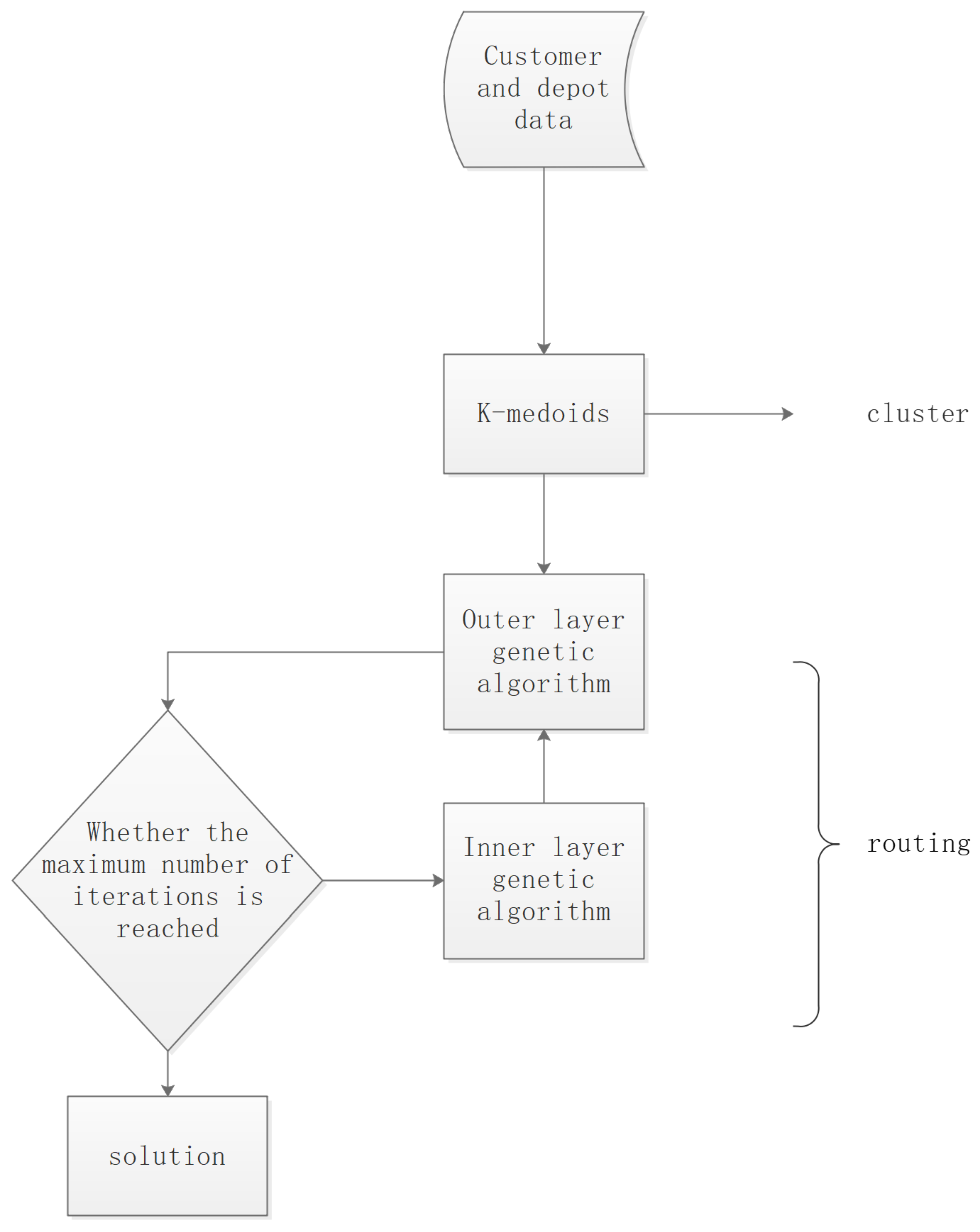
In this study, the proposed algorithm adopts an internationally recognized concept: transforming the multi-depot routing-distribution problem into multiple single-depot path-distribution problems and then planning for each single-network path-distribution problem to find the best path, that is, the cluster first and then the route method.
To calculate the appropriate departure time, Ibaraki [44] proposed that for a given order, a better solution can be obtained by using an analysis method, which effectively solved the problem. However, the transmission time between two points is not fixed because of the time-varying speed used in this study, so using the above method to obtain the solution is difficult; therefore, the use of a heuristic algorithm is more conducive to the solution of the algorithm.
Traditional algorithms always produce the optimal solution [45]. However, it is difficult for a traditional algorithm to find a solution owing to several constraints of the problem. Therefore, this study improved the genetic algorithm to obtain a dual-layer genetic algorithm. Genetic algorithm uses the coding of decision variables as the operation object and can directly operate on a variety of different structures. This makes the genetic algorithm easier to expand and use.
Figure 2 illustrates the flow of the algorithm.

4.1. Customer Clustering

Most of existing problems on vehicle routing with time windows only consider the effect of spatial distance when clustering delivery customers, but not the effect of time windows. In the subsequent planning process, if a customer and his subsequent customers are spatially close to each other, the time windows that are far apart can also lead to an increase in cost and even infeasible solutions. In this study, we consider the influence of both time and space on the clustering results and adopt the measure of spatio-temporal distance proposed by Wang et al. [46] to calculate the distance between customer nodes.

4.1.1. Temporal-Spatial Distance

The time distance here is not used to calculate the similarity of the time windows of the two nodes. It is used to calculate whether there can be a smaller time window penalty from the first node to the second node if two nodes are adjacent. This can reduce the cost of the delayed or early arrival of nodes in a cluster.
The method proposed by Wang et al. [46] divides the time-window distance into four cases. This study assumes that the time window of node i is [ E T i , L T i ] and that of node j is [ E T j , L T j ] . Then, the travel time between nodes ij t i j = d i j v . Assume that the vehicle is now located at node i and the moment of arrival at node i is t i k a and t i k a [ E T i , L T i ] . Then, the vehicle arrives at node j at moment t j k a and lies between the interval [ E T i + t i j + t i s , L T i + t i j + t i s ] . Use [a,b] to represent the interval above.
Then, the comparison between the two intervals is divided into four cases: a set all greater than another set, a set all smaller than another set, a set with intersection, and a set all located inside another set. In the following section, the time distance represented by each of the four cases is described in detail:
1.
The first case is when one set is larger than the other, which means that the maximum value in one set is smaller than the minimum value in the other set. The maximum value b is smaller than the earliest arrival time E T j in time window [ E T j , L T j ] of node j, as shown in Figure 3, indicating starting from node i will inevitably arrive at node j in advance. Then, the time distance between node i and node j is c 1 ( E T j b ) .
2.
The second case is where one set is smaller than the other; that is, the minimum value of one set is larger than the maximum value of the other set. Here, it represents the minimum value a is greater than the latest arrival time L T j , as shown in Figure 4. This indicates that it is necessarily late from node i to node j. Then, the time distance between node i and node j is c 2 ( a L T j ) .
3.
The third case is where the two sets have intersecting parts. It signifies the relationship between the time interval t j k a = [a,b] and the time window [ E T j , L T j ] of node j: a [ E T j , L T j ] , b > L T j or b [ E T j , L T j ] , a < E T j , as shown in Figure 5. Then, the spatial distance between node i and node j in this case is c 3 ( t i j + t i s ) .
4.
The last case is the best case, where one set contains another set. It means that [ a , b ] [ E T j , L T j ] , which implies that the time when the vehicle starts from node i and arrives at node j must be in the time window [ E T j , L T j ] of node j, as shown in Figure 6. The time distance in this case is t i j + t i s .
The above four cases are summarized in a complete formula, as expressed in Equation (21).
D i j t = c 1 ( E T j b ) E T j > b c 2 ( a L T j ) a > L T j c 3 ( t i j + t i s ) a < E T j < b o r a < L T j < b t i j + t i s E T j < a < b < L T j
Since the temporal distance is directional, i.e., D i j t D j i t , the greater of the two is utilized as the temporal distance between node i and node j.
The spatial distance D i j s between nodes i and j was then calculated using the simplest Euclidean distance.
This study standardized the time and space distance to facilitate the subsequent calculation of the space-time distance because time and space are measured in different ways. Thus, the final spatio-temporal distance between node i and node j is shown in Equation (22).
D i j = α 1 × ( D i j s min m , n C , m n D m n s ) ( max m , n C , m n D m n s min m , n C , m n D m n s ) + α 2 × ( D i j t min m , n C , m n D m n t ) ( max m , n C , m n D m n t min m , n C , m n D m n t ) , α 1 + α 2 = 1 , i , j C

4.1.2. K-Medoids Clustering Algorithm

The optimal solution of each subpath is different, and the final solution results are also different. Therefore, an efficient, accurate, and reasonable partitioning method is essential to solving the entire problem. A suitable partitioning algorithm can also reduce the computational effort of the entire problem, thereby reducing the time required for the entire solution process. The problem to be solved in this study is the multi-depot vehicle path problem with a vehicle time window with an elective waiting strategy, which must satisfy the following by the first part of the partitioning. The customers in each partitioned sub-region do not overlap; the customer points located in the same sub-region are relatively concentrated, thus saving transportation time and cost; and the load in each interval should be approximately the same to avoid a region with a particularly high demand of the situation.
The basic idea of the K-medoids algorithm is that, given the initial customers’ clustering centroids, the customer points closest to them are grouped. The values of the cluster centers are continuously updated using an iterative method until the best clustering result is obtained [47]. The traditional K-medoids algorithm has difficulty to solve large-scale data, although it is the most famous divisional clustering algorithm and the most widely used of all clustering algorithms owing to its simplicity and efficiency. This study uses a solution based on the genetic algorithm clustering proposed by Qi et al. [48] to perform the clustering operation. The objective function is expressed in Equation (23).
min F = i = 1 k j a s s i g n e d t o i D i j
Because specific load constraints are not considered in clustering, some clusters with demands exceeding the maximum load of vehicles will occur; thus, the clustering results will be optimized. Set up a virtual car park D 0 , start visiting from the customer closest to the virtual car park in each cluster, and visit the next customer point according to the spatio-temporal distance. Finally, if the remaining capacity is no longer sufficient to satisfy any of the remaining customers, then the remaining customers will go to see whether the neighboring clusters can satisfy the remaining customers according to the nearest principle. If so, the customer point is categorized into neighboring clusters, and then loop this operation for all clusters. Finally, a clustering result that satisfied the vehicle constraint was obtained.

4.2. Outer Layer Genetic Algorithm

The classical genetic algorithm is very effective for solving NP-hard problems [49,50,51]. However, it seems a bit overwhelming to solve optimization problems with multiple constraints, and not easy to obtain stable and efficient solutions. Therefore, the two-layer genetic algorithm proposed in this paper presents a more effective solution to this class of problems. The two-layer genetic algorithm is characterized by the outer layer providing specific conditions and parameters for the inner layer and the inner layer returning partial results to the outer layer. The two-layer genetic algorithm used in this problem is roughly described as follows: the outer layer genetic algorithm generates the distribution path scheme, the inner layer provides the optimal time sequence with the minimum cost for each distribution scheme with an elective waiting strategy, and the minimum cost is returned to the outer layer as the outer adaptation degree to select the optimal distribution scheme. The whole algorithm is shown in Algorithm 1.
A GA is an evolutionary algorithm [52,53,54,55,56] that finds the optimal solution by imitating the selection mechanism and heredity in nature. However, they are prone to premature convergence and fall into locally optimal solutions. The variable neighborhood search (VNS) algorithm searches all solutions using various domain structures and has the function of jumping out for locally optimal solutions and accelerating convergence for other solutions [42]. Here, a combination of both was used to optimize the outer distribution-path scheme problem.
Algorithm 1: Dual-layer genetic algorithm
Require: Out_pop_size: Outer layer population size
Require: Out_max_iter: Outer layer maximum number of iterations
Require: Inner_max_iter: Inner layer maximum number of iterations
Require: Inner_pop_size: Inner layer population size
Require: N k = { N 1 , N 2 , N m } : neighborhood structure N m is the mth neighborhood structure
1:
Initialize pop_0;Generate initialized populations
2:
for g e n = 1 to O u t _ p o p _ i t e r  do
3:
   for  i = 1 to O u t _ p o p _ s i z e  do
4:
     Initialize timelist_0;Generate initialized Waiting time series
5:
     for  j = 1 to I n n e r _ m a x _ i t e r  do
6:
        calculate the fitness timelist_j-1;Calculate the cost of the ith individual on the set of waiting times
7:
        select timelist_j from timelist_j-1;Select elite retention and roulette strategies
8:
        crossover_mutate timelist_j
9:
     end for
10:
     Best fitness with waiting strategy
11:
   end for
12:
   select pop_gen from pop_gen-1;Select elite retention and roulette strategies
13:
   crossover pop_gen;
14:
   for  i = 1 to O u t _ p o p _ s i z e  do
15:
     for  j = 1 to M A X _ N  do
16:
        pop_gen(i) disturbed from the first neighborhood structure N 1
17:
        Initialize timelist_0;Generate initialized Waiting time series
18:
        for  j = 1 to I n n e r _ m a x _ i t e r  do
19:
          calculate the fitness timelist_j-1;Calculate the cost of the neighborhood of the ith individual on the set of waiting times
20:
          select timelist_j from timelist_j-1;Select elite retention and roulette strategies
21:
          crossover_mutate timelist_j
22:
        end for
23:
        Best fitness with elective waiting strategy
24:
        if  p p 0  then
25:
          pop_gen(i) = pop_gen_ N 1 (i)
26:
          break
27:
        end if
28:
        pop_gen(i) continues to be disturbed by the next neighborhood structure N m
29:
        repeat
30:
     end for
31:
   end for
32:
end for
33:
Best solution

4.2.1. Encode and Decode

In the chromosome coding approach used in this study, the chromosome consists of genes, that is, C h r o m = { G 1 , , G n } , where n refers to the number of regions divided. Each gene is composed of all clients of a subregion, and each gene G i { i ( 1 , 2 , , n ) } represents the path-planning result for each subregion. The gene G i is encoded by a set of integers, and inside it is the distribution sequence consisting of the customers of the region.
As shown in Figure 7, the chromosome represented here has ten customer points, and this chromosome has a total of four genes, from which the whole network can be divided into four sub-regions. G 1 contains three customer points, 4, 5, and 3, and in this chromosome the order of customer access is first from the depot to visit node 4, then visit node 5, and finally visit node 3 and return to the depot.
Chromosomes alone are not sufficient because it is not yet known from which depot and back to which each car leaves, so a decoding operation is needed for chromosomes. The main task of the decoding process is to assign the starting and ending depots of each gene to the corresponding gene so that the entire chromosome becomes a feasible solution. The strategy used in this study is to assign the closest car yard to the first and last client in the gene according to the proximity principle and insert it into the first and last position of the gene. A valid solution is shown in Figure 8.

4.2.2. Crossover

With continuous research, there are various crossover operators about genetic algorithms, except for the common one- and two-point crossovers. The above-mentioned methods are simple and can yield good results for some simple problems. However, in our problem, infeasible paths were often generated. Therefore, this study uses the ordered crossover (OX) method to perform cross operations.
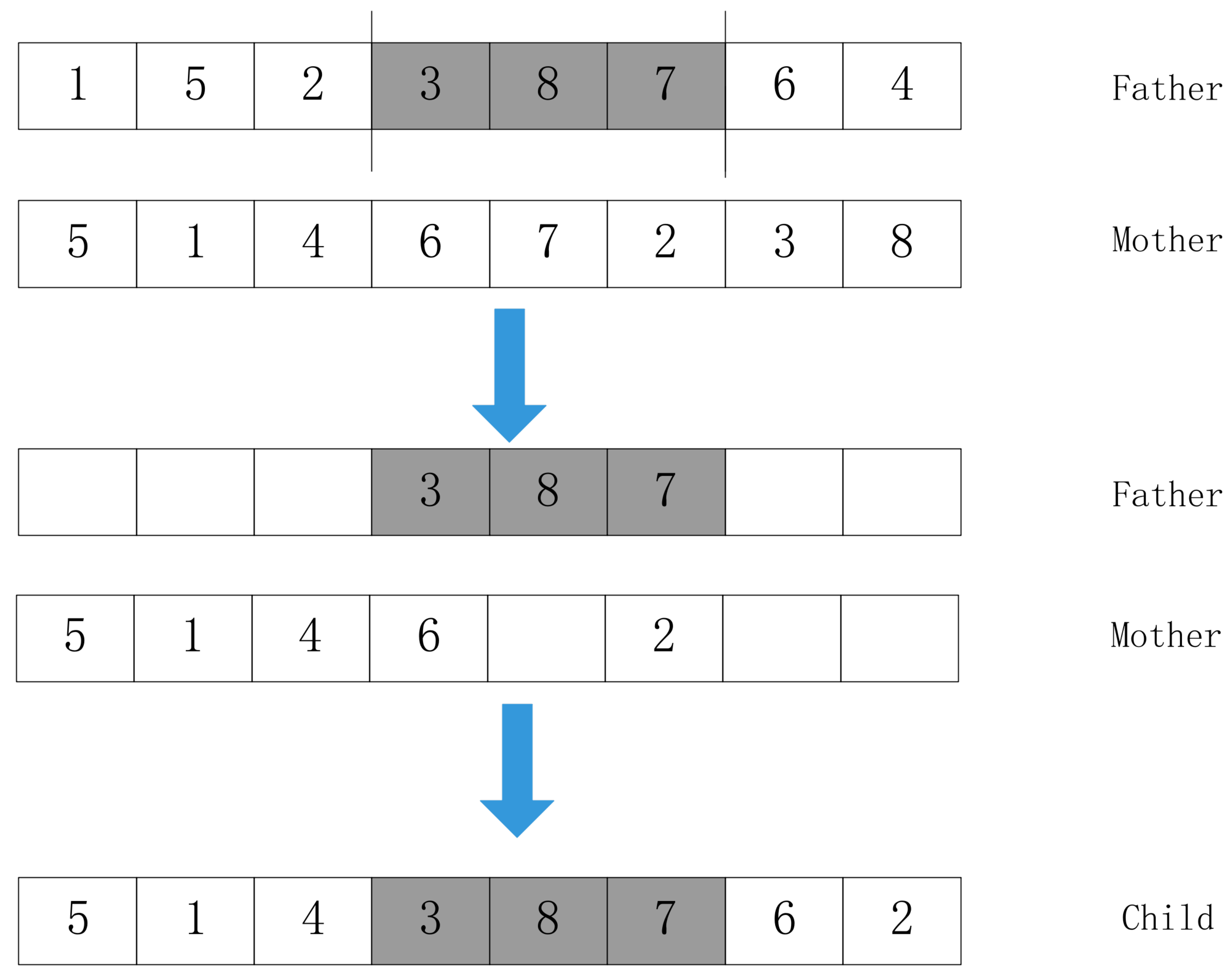
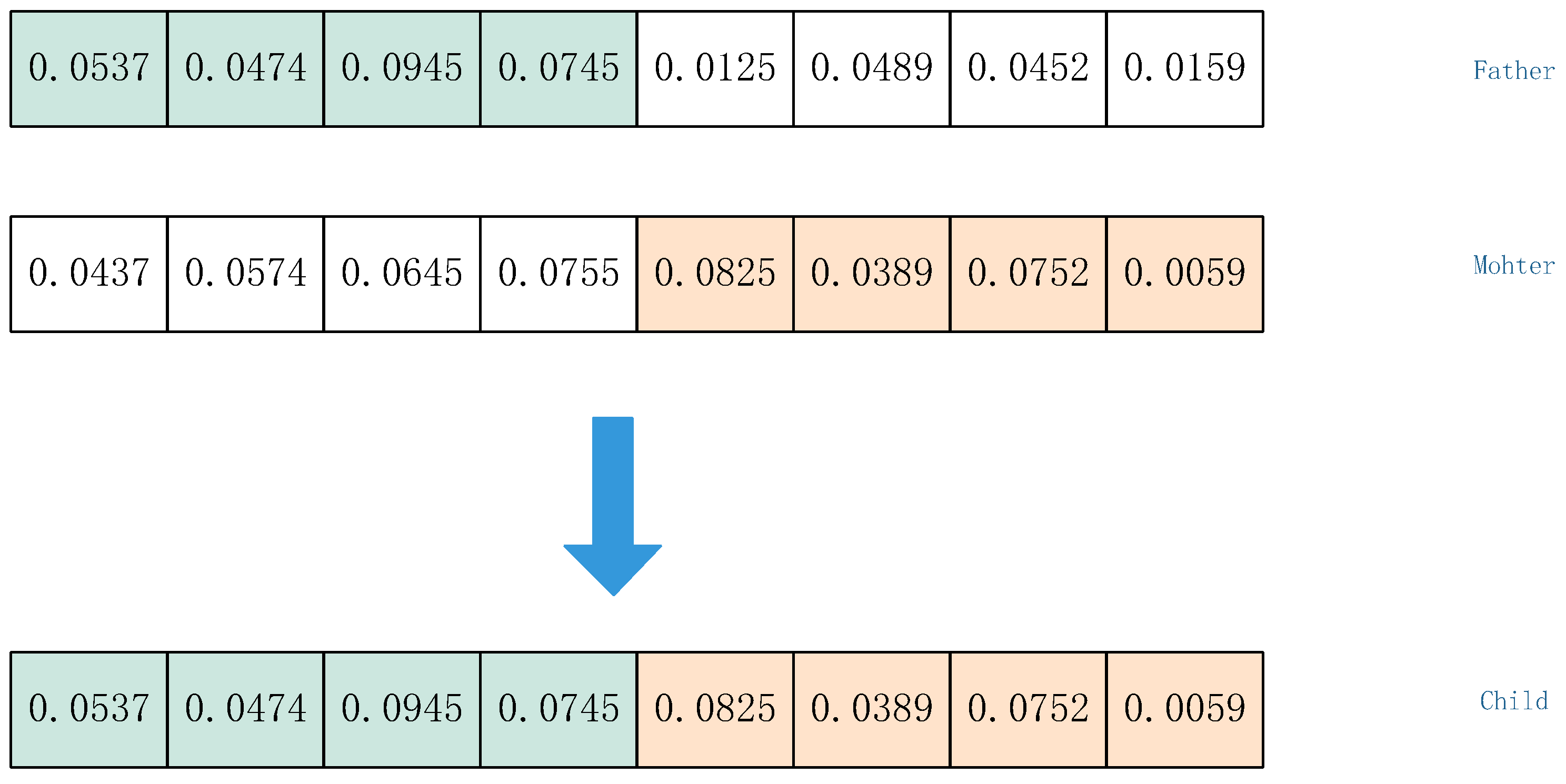
The first step is to select two individuals at random from the population and use an ordered crossover for each gene in parallel. Ordered crossover (OX) is also available in various versions, so the specific operation used in this study is as follows. First, two customers are selected at random from the path, which can be the same or different. Then, the point between the two customers of the father is saved in the same position as the child, and the other customer points are placed in the corresponding positions of the child at one time in the order of the mother. The following is an example that illustrates this, as shown in Figure 9.
In Figure 9, customer points 3 and 7 are the endpoints of the retention interval. Hence, the customer points in the parent generation will be saved to the same location as the child generation without change. That is, customer points 3, 8, and 7 are saved to the corresponding location of the child as is. The sub generation still lacks five customer points 1, 5, 2, 6, and 4. Delete customer points 3, 8, and 7 in the mother generation, and place the remaining nodes in the blank position of the child generation one by one in order.

4.2.3. Local Search

In this study, the local search algorithm plays an important role in preventing the situation from falling into a local optimum, such as the genetic algorithm, and is an effective means to drive the algorithm to continuously find the best. The proposed algorithm adopts the concept of VNS to deal with a local search.
1.
Neighborhood structure
(a)
Exchange
Arbitrarily select two customer points i and j, and then swap the positions of the two. As shown in Figure 10.
(b)
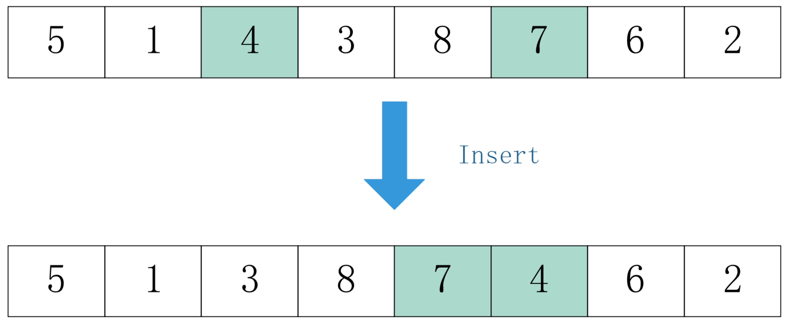
Insert
Select two customer points i and j randomly and insert customer point i after the customer point. As shown in Figure 11.
(c)
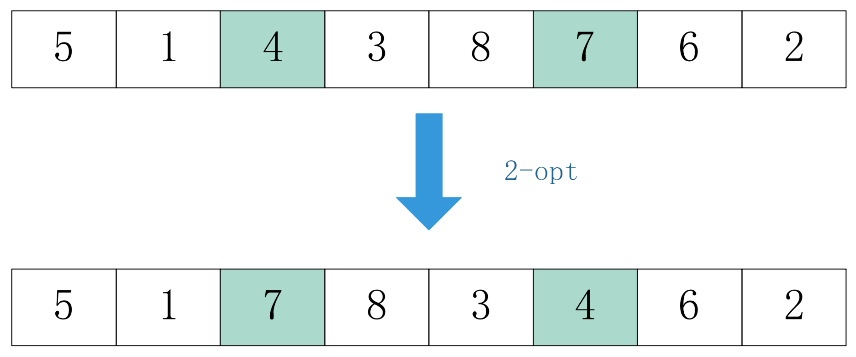
2-opt
Arbitrarily select two client points i and j, and then invert the interval between these two points. As shown in Figure 12.
2.
Solution acceptance
This study used an acceptance mechanism similar to simulated annealing to prevent the algorithm from falling into local optima while expanding the search space. If the solution after the neighborhood is better adapted than the itself, then it is replaced. Otherwise, the worse solution is accepted according to a certain probability. The solution acceptance formula is shown in Equation (24). Here, f x refers to the current chromosome fitness, where f x is the chromosome fitness after the neighborhood, fitness is obtained using an inner-layer genetic algorithm, and iter is the number of current iterations.
p = 1 f x < f x e x p ( f x f x i t e r ) f x f x

4.2.4. Select Operation

The selection operations in both the inner and outer layers use a combination of elite retention and roulette; that is, the optimal chromosome is first preserved in the offspring, and then the other chromosomes are inherited into the progeny based on fitness probabilities using the roulette. This paper takes fitness as the reciprocal of the total cost and transforms the minimization problem into the maximization problem to use roulette strategy.

4.3. Inner Layer Genetic Algorithm

The internal genetic algorithm is designed to find the best waiting time while making the total cost smaller. Therefore, for each path, it is necessary to determine the waiting time that minimizes the cost of the path under the maximum waiting time constraint. Because the internal genetic algorithm only calculates the waiting time on a single path, the problem is solved on a small scale; therefore, the internal layer uses a genetic algorithm, which has good scalability, strong robustness, and is convenient to connect with the external algorithm.

4.3.1. Encode and Decode

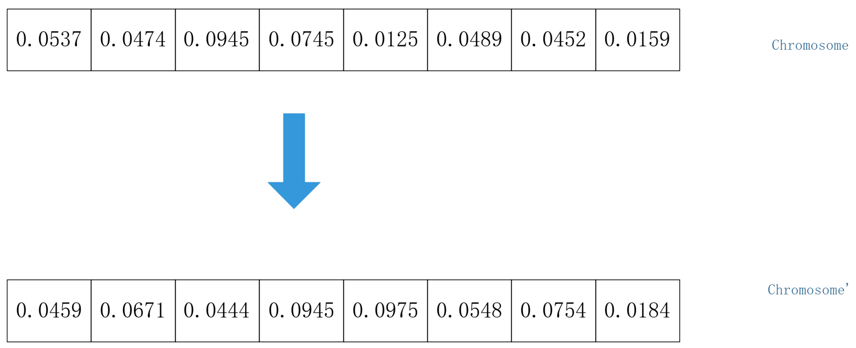
Here, we use the floating-point coding method. In this study, we set the maximum waiting time W to 0.1 h. Each gene represents the waiting time for each path under the maximum waiting time constraint, as illustrated in Figure 13.
We know that every two points will generate a path. The number of paths is equal to the number of nodes minus one, with the depot at the beginning and end of the path. Then, each path will decide whether to wait, so the length of the chromosome represents the total number of paths. As shown in Figure 13, there are eight waiting decision variables; therefore, this chromosome represents a route with eight sub-paths. Therefore, it can be inferred that there are nine nodes: seven customer nodes and two depot nodes.

4.3.2. Crossover and Mutation

Single-point crossover method is used to select any position in the chromosome and merge the chromosome part before this point in the father with the chromosome after this point in the mother to form offspring, as shown in Figure 14.
The mutation operator first determines whether a chromosome is subject to mutation, then randomly generates a set of floating-point numbers satisfying the maximum waiting time constraint to replace the floating-point number at the chromosome, as shown in Figure 15.
Since the crossover mutation operator here is the most basic method, it will not be further introduced.

5. Experiment

This section presents some of the DGAVNS proposed in this study for evaluating the W-MDVRPTW problem. The algorithms in this study were implemented in MATLAB 2021b, compiled, and run on a Windows 10 operating system using an Intel Core i5-9500 processor system at 3.00 GHz with 8 GB RAM.
Since there is no dataset matching this article, this article chooses to modify common datasets. The case used in this study was adapted from the example of MDVRP proposed by Cordeau et al. [57]. The coordinate positions of each dataset are preserved, and the demand is generated by taking a random decimal in the interval [0, 1] and then randomly adding or subtracting 0.05. The time window is generated by randomly generating an integer in the interval [6, 18] and then randomly adding or subtracting 0.5, and the service time is 0.5 of the demand times the demand. The specific information is shown in Table 2.
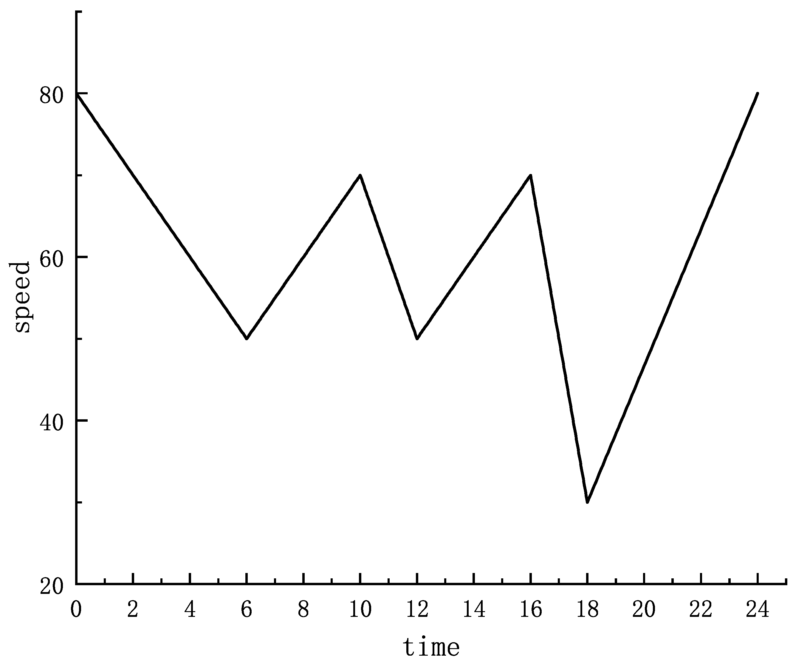
Here, we modified the speed model proposed by Horn [21] to obtain the speed model used in this study. Figure 16 illustrates the time-varying speed function.
First, we will discuss the internal genetic algorithm. First, we conducted an experimental analysis of different mutation rates. We set I n n e r _ p o p _ s i z e = 50 , I n n e r _ m a x _ s i z e = 1000 , and calculate a path [9, 30, 33, 39, 44]. We conducted 50 experiments using different mutation parameters and compared their average values. The crossover rate is fixed at 0.9, and the comparison chart of different mutation rates is shown in Figure 17. The figure clearly shows that when the mutation rate is 0.2, it has a better fitness, so the mutation rate is fixed at 0.2 for later experiments.
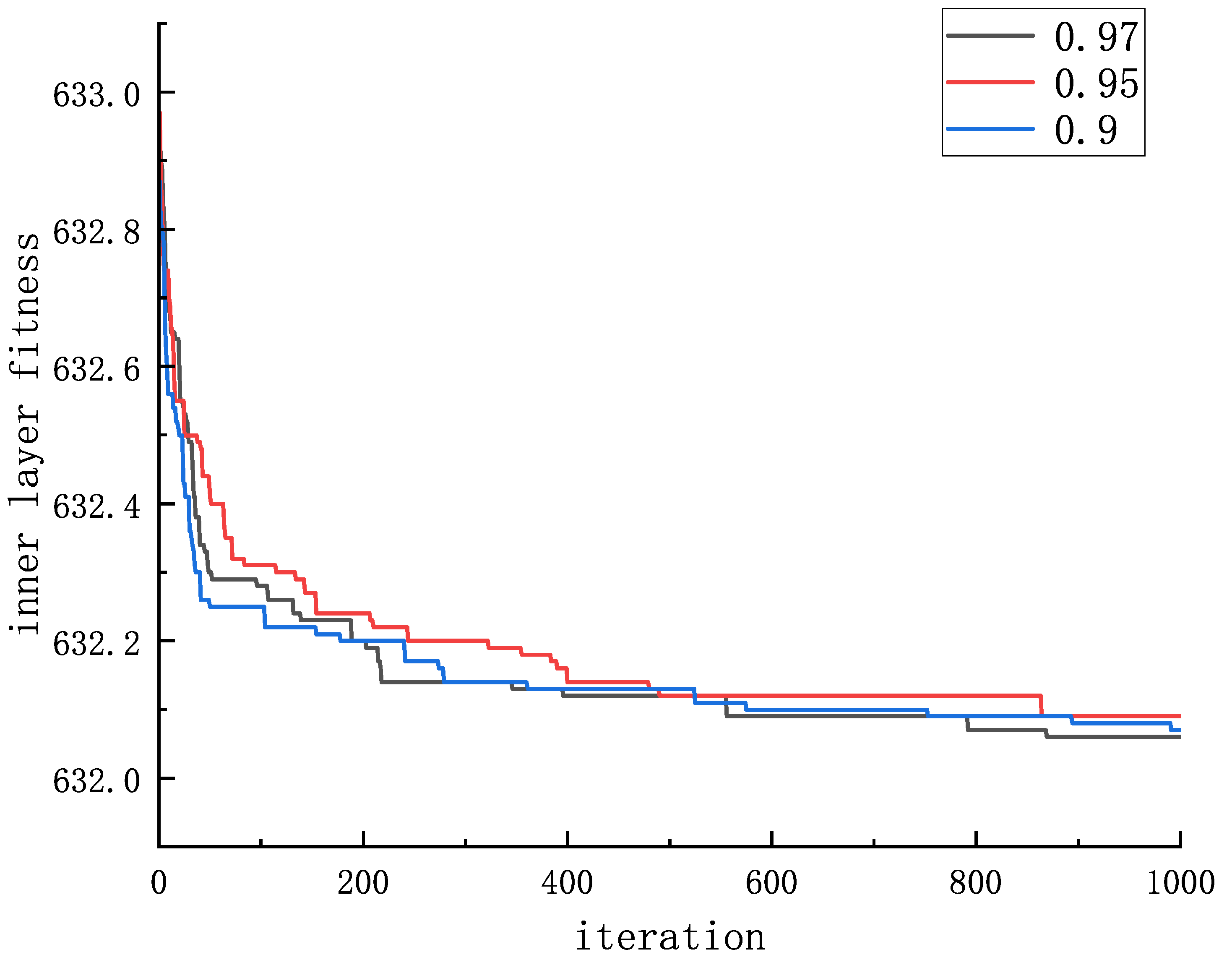
Then, the fixed mutation rate is 0.2, and the average values of 50 experiments with different crossover rates are compared. The results are shown in Figure 18. Evidently, it has good fitness when the crossover rate is 0.97.
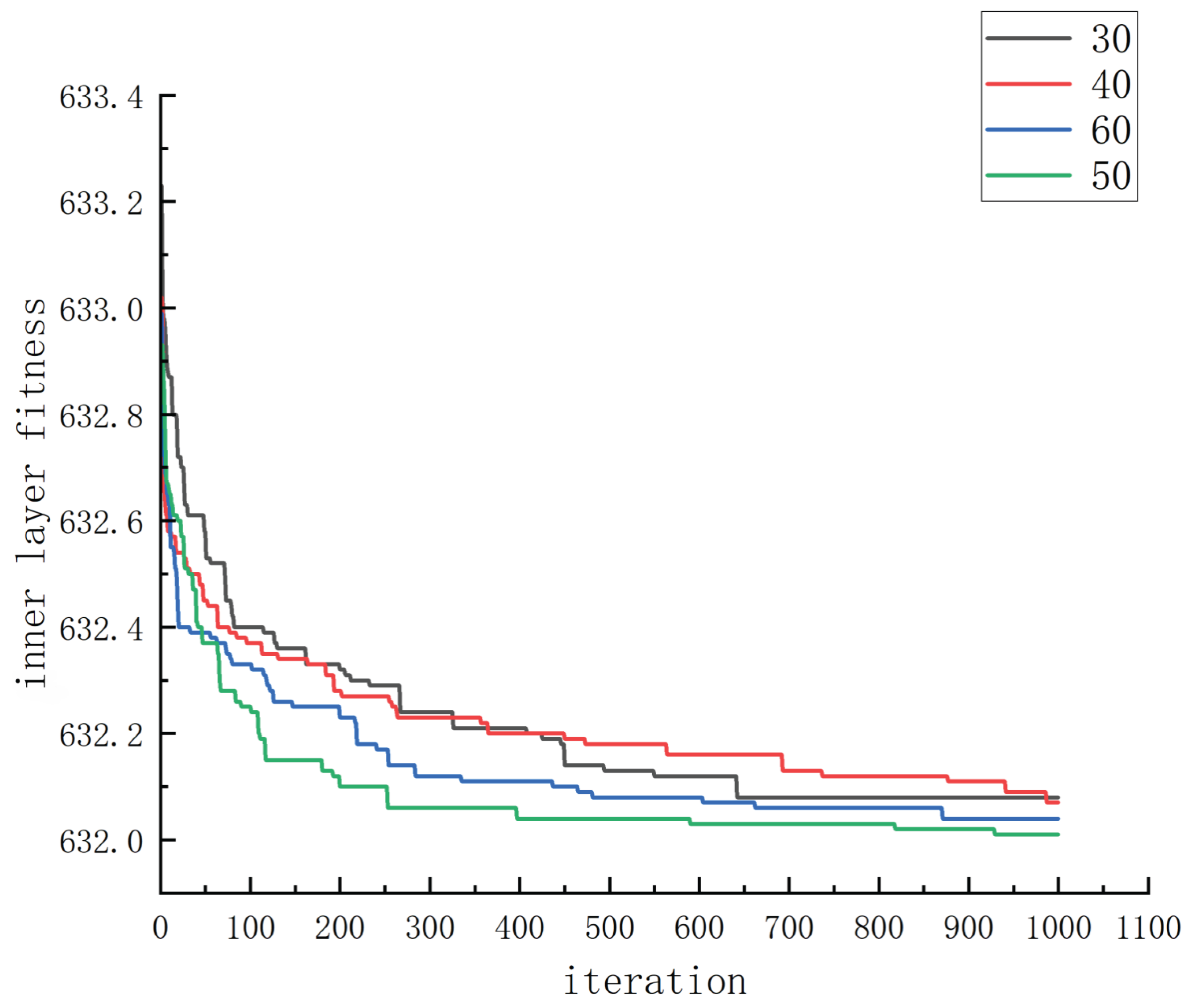
However, in the above comparison, the number of iterations is set to 1000. The running time reached 7 s because the internal genetic algorithm needs to continuously solve the integral and function. However, this is only the calculation time for a single path. For the outer-layer genetic algorithm, a chromosome represents all paths in the entire path network. Assuming that the number of outer paths is 5, the number of outer populations is 50, and the number of outer iterations is 200, the operation time of the outer layer is not included. The time required to calculate the fitness of each path is only 7 × 5 × 50 × 200 = 35 , 000 s = 97.2 h, which is much more than expected. As shown in Figure 18, when the number of iterations is 100, the fitness of the red curve reaches 632.2, while it only decreases by 0.2 yuan from 100 to 1000 generations, and it only takes 1 s to reach 100 generations. The above time becomes 1 × 5 × 50 × 200 = 13 h. At this time, the time remains large. However, from the characteristics of the genetic algorithm, there are duplicate genes and chromosomes in each population. In addition, there are an increasing number of repeated calculations in the later iteration stage. Therefore, in this study, a global variable is set to save the calculated path fitness to accelerate the algorithm. According to the experimental test, the proportion of fitness calculated using the internal genetic algorithm again accounts for only 2%, 2 % × 13 h = 15 min. The running time of the algorithm is reduced by reducing the number of iterations and setting the global variables, and the efficiency of the algorithm is improved.
Next, the influence of different population numbers on fitness is discussed. The crossover rate was set to 0.97, the mutation rate was set to 0.2, and 50 experiments were performed on different populations to obtain the average value, as shown in Figure 19. From the figure, when the population sizes are 50 and 60, the fitness values are close. Therefore, a population size of 50 was selected to save operation time and memory space.
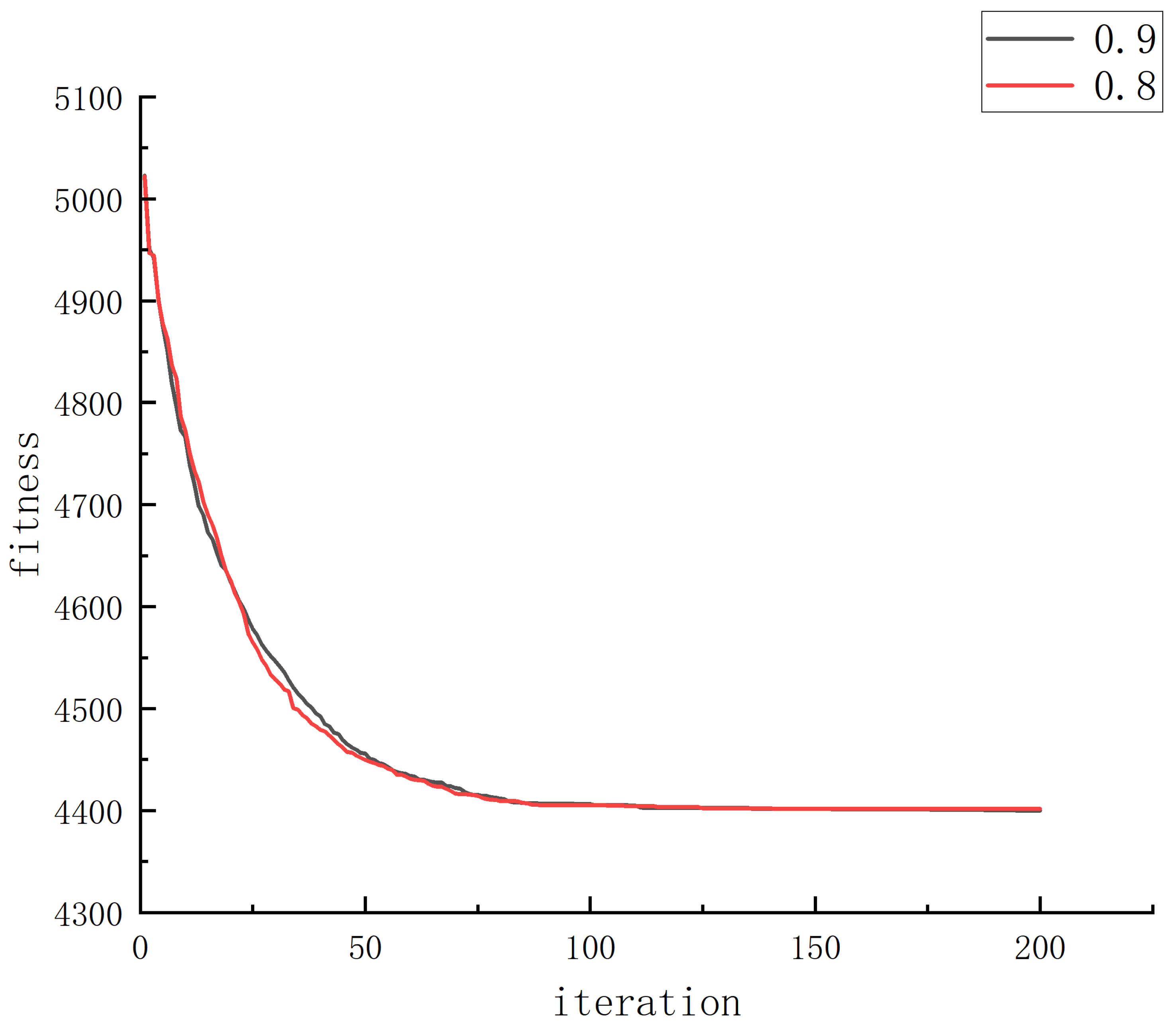
After discussing the inner layer genetic algorithm, the outer layer genetic algorithm is discussed. The outer-layer genetic algorithm removes the mutation operation and individual transformation using a neighborhood search. Therefore, only the impact of different crossover rates on the outer-layer genetic algorithm is discussed. The results are shown in Figure 20. It is found that the results of 0.8 and 0.9 are the same. Thus, 0.9 is used here as the crossover rate.
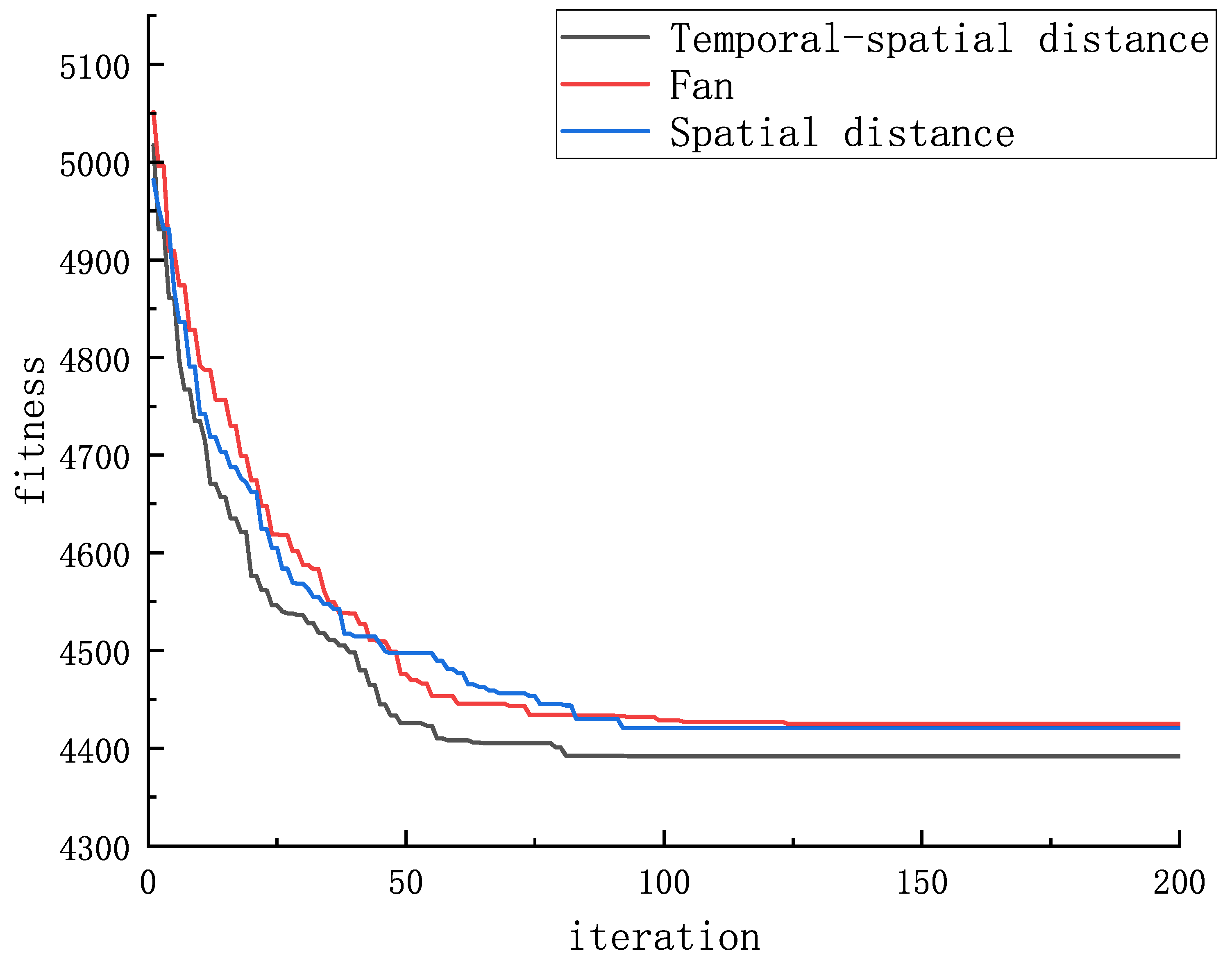
The algorithm proposed in this paper is based on the a hybrid genetic algorithm with variable neighborhood search considering the temporal-spatial distance (HGAVNS_TS) algorithm proposed by Fan [42]. The effectiveness of the algorithm has been effectively proved by Fan [42], so here only compare it with HGAVNS_TS. Similarly, here we compare only considering the space distance to ensure the effectiveness of this algorithm. The parameters of the algorithm are set as follows: O u t _ p o p _ s i z e = 20 , O u t _ m a x _ i t e r = 150 , Q = 5 , W = 0.1 , p = 0.99 . First, 50 iterations were conducted for each algorithm to compare the average values. The results are presented in Figure 21. The cost of adopting the selective waiting strategy is reduced by about one percent compared with the cost of non-waiting. Because this article limits the waiting time to 0.1 h, the cost reduction is not obvious, but it also shows that the optional waiting strategy can effectively reduce the delivery cost.
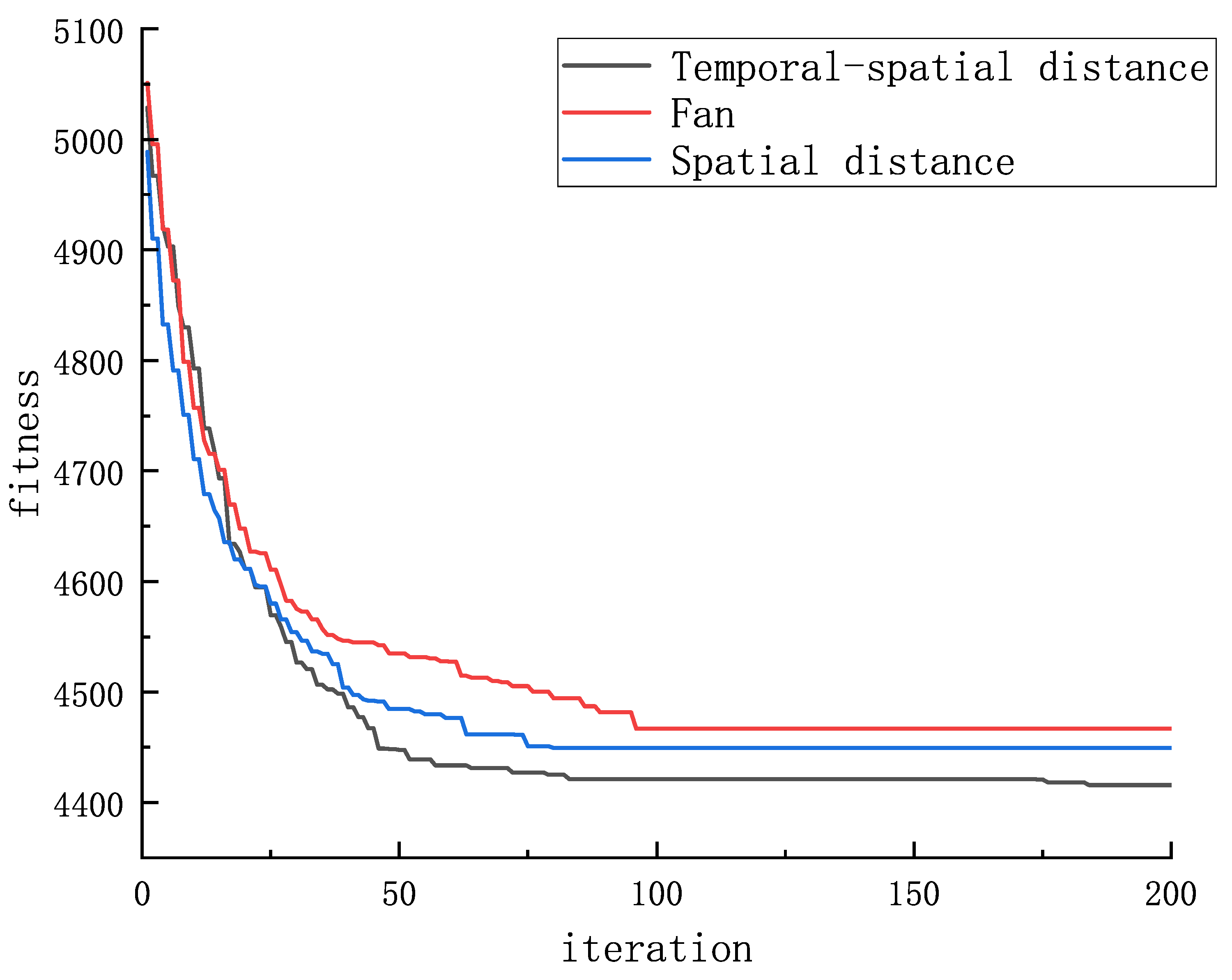
Figure 22 is the comparison chart of the iteration curve with the lowest cost, and Figure 23 is the comparison chart of the iteration curve with the highest cost.

6. Conclusions

In today’s e-commerce platforms, multi-depot shipping has become an advantage for merchants. Most companies choose to disperse their depots to different locations for the timely and prompt shipping, as well as cost reduction. In the real world, traffic conditions are also constantly changing. Therefore, considering this factor and seeking a better allocation scheme, this paper proposed an MDVRPTW problem with an elective waiting policy. A mixed-integer programming model was proposed based on the proposed problem, and a two-layer genetic algorithm was proposed to solve this problem. In this study, multiple-route genes were encoded by forming a chromosome. In this case, it is more intuitive and convenient to obtain specific routes from a chromosome. In addition, the use of simulated annealing for the reception of the solution combined with the search method of VNS allows the algorithm to accelerate convergence without falling into a local optimum solution. Experiments demonstrate that the proposed algorithm can effectively solve the proposed problem.
The proposed problem extends the common MDVRPTW problem, making it more realistic. Simultaneously, it can reduce the distribution cost to increase the profit of the enterprise, providing a feasible solution to the distribution problem of multi-depot enterprises.
The shortcomings of this paper are also evident. When solving the inner genetic algorithm, the algorithm is not iterated to stable convergence, but is limited to 100 generations, which effectively reduces the calculation time, but also makes the algorithm unstable and unable to converge. Simultaneously, a heuristic algorithm is used to calculate the fitness of the inner layer. The greatest disadvantage of the heuristic algorithm is that it is unstable. Therefore, the solutions obtained vary within a range, resulting in different fitness values for the same chromosome at different calculation times. In addition, the results of the first solution were saved for subsequent use instead of repeated calculations for the same path to reduce the calculation time. It will also lead to the limitation of the required fitness.
In future work, determining the appropriate maximum waiting time to make it more suitable for real situations will be a new problem. Solving the waiting time stably and quickly is also an important problem.

Author Contributions

Conceptualization, C.-M.C. and S.L.; methodology, C.-M.C. and S.L.; Software, S.L.; validation, J.N. and J.M.-T.W.; formal analysis, S.L. and J.M.-T.W.; investigation, J.N.; writing–original draft preparation C.-M.C., S.L., J.N. and J.M.-T.W.; Visualization: S.L. and J.N.; supervision, C.-M.C.; project administration, J.M.-T.W.; funding acquisition, J.N. All authors have read and agreed to the published version of the manuscript.

Funding

This research was funded by GraceChain Software Ltd-SDUST-GLOBAL OPTIMUM FRESH Cross-Border Fresh Supply Chain Platform joint research project.

Institutional Review Board Statement

Not applicable.

Informed Consent Statement

Not applicable.

Data Availability Statement

Not applicable.

Conflicts of Interest

The authors declare no conflict of interest.

References

  1. De, A.; Mamanduru, V.K.R.; Gunasekaran, A.; Subramanian, N.; Tiwari, M.K. Composite particle algorithm for sustainable integrated dynamic ship routing and scheduling optimization. Comput. Ind. Eng. 2016, 96, 201–215. [Google Scholar] [CrossRef]
  2. De, A.; Gorton, M.; Hubbard, C.; Aditjandra, P. Optimization model for sustainable food supply chains: An application to Norwegian salmon. Transp. Res. Part Logist. Transp. Rev. 2022, 161, 102723. [Google Scholar] [CrossRef]
  3. Wu, Z.; Gao, Q.; Jiang, B.; Karimi, H.R. Solving the production transportation problem via a deterministic annealing neural network method. Appl. Math. Comput. 2021, 411, 126518. [Google Scholar] [CrossRef]
  4. Hardcastle, J. Walmart, General Mills, Anheuser-Busch improve freight efficiency, cut emissions. Environ. Lead. 2015. Available online: http://www.en-vironmentalleader.com/2015/05/13/walmart-general-mills-anheuser-busch-improve-freight-efficiency-cut-emissions/#ixzz473YFXy9e (accessed on 13 May 2015).
  5. Wu, Z.; Karimi, H.R.; Dang, C. A deterministic annealing neural network algorithm for the minimum concave cost transportation problem. IEEE Trans. Neural Netw. Learn. Syst. 2019, 31, 4354–4366. [Google Scholar] [CrossRef]
  6. Namasudra, S.; Sharma, P. Achieving a decentralized and secure cab sharing system using blockchain technology. IEEE Trans. Intell. Transp. Syst. 2022, 1–10. [Google Scholar] [CrossRef]
  7. Pan, J.S.; Lv, J.X.; Yan, L.J.; Weng, S.W.; Chu, S.C.; Xue, J.K. Golden eagle optimizer with double learning strategies for 3D path planning of UAV in power inspection. Math. Comput. Simul. 2022, 193, 509–532. [Google Scholar] [CrossRef]
  8. Li, Z.; Miao, Q.; Chaudhry, S.A.; Chen, C.M. A provably secure and lightweight mutual authentication protocol in fog-enabled social Internet of vehicles. Int. J. Distrib. Sens. Netw. 2022, 18, 15501329221104332. [Google Scholar] [CrossRef]
  9. Rezaei, N.; Ebrahimnejad, S.; Moosavi, A.; Nikfarjam, A. A green vehicle routing problem with time windows considering the heterogeneous fleet of vehicles: Two metaheuristic algorithms. Eur. J. Ind. Eng. 2019, 13, 507–535. [Google Scholar] [CrossRef]
  10. Liu, C.; Kou, G.; Zhou, X.; Peng, Y.; Sheng, H.; Alsaadi, F.E. Time-dependent vehicle routing problem with time windows of city logistics with a congestion avoidance approach. Knowl.-Based Syst. 2020, 188, 104813. [Google Scholar] [CrossRef]
  11. Xiao, Y.; Konak, A. The heterogeneous green vehicle routing and scheduling problem with time-varying traffic congestion. Transp. Res. Part E Logist. Transp. Rev. 2016, 88, 146–166. [Google Scholar] [CrossRef]
  12. Bektaş, T.; Laporte, G. The Pollution-Routing Problem. Transp. Res. Part B Methodol. 2011, 45, 1232–1250. [Google Scholar] [CrossRef]
  13. Kuo, Y.; Wang, C.C.; Chuang, P.Y. Optimizing goods assignment and the vehicle routing problem with time-dependent travel speeds. Comput. Ind. Eng. 2009, 57, 1385–1392. [Google Scholar] [CrossRef]
  14. Ichoua, S.; Gendreau, M.; Potvin, J.Y. Vehicle dispatching with time-dependent travel times. Eur. J. Oper. Res. 2003, 144, 379–396. [Google Scholar] [CrossRef] [Green Version]
  15. Mu, D.; Wang, C.; Wang, S.; Zhou, S. Solving TDVRP based on a parallel-simulated annealing algorithm. Comput. Integr. Manuf. Syst. 2015, 21, 1626–1636. [Google Scholar] [CrossRef]
  16. Ma, X.; Liao, L.; Li, Z.; Lai, R.X.; Zhang, M. Applying Federated Learning in Software-Defined Networks: A Survey. Symmetry 2022, 14, 195. [Google Scholar] [CrossRef]
  17. De, A.; Wang, J.; Tiwari, M.K. Hybridizing Basic Variable Neighborhood Search With Particle Swarm Optimization for Solving Sustainable Ship Routing and Bunker Management Problem. IEEE Trans. Intell. Transp. Syst. 2020, 21, 986–997. [Google Scholar] [CrossRef]
  18. Beasley, J. Adapting the savings algorithm for varying inter-customer travel times. Omega 1981, 9, 658–659. [Google Scholar] [CrossRef]
  19. Wright, G. Scheduling of Vehicles from a Central Depot to a Number of Delivery Points. Oper. Res. 1964, 12, 568–581. [Google Scholar] [CrossRef]
  20. Hill, A.V.; Benton, W.C. Modelling Intra-City Time-Dependent Travel Speeds for Vehicle Scheduling Problems. J. Oper. Res. Soc. 1992, 43, 343–351. [Google Scholar] [CrossRef]
  21. Horn, M.E.T. Efficient modeling of travel in networks with time-varying link speeds. Networks 2015, 36, 80–90. [Google Scholar] [CrossRef]
  22. Jie, K.W.; Liu, S.Y.; Sun, X.J. A hybrid algorithm for time-dependent vehicle routing problem with soft time windows and stochastic factors. Eng. Appl. Artif. Intell. 2022, 109, 104606. [Google Scholar] [CrossRef]
  23. Bai, Q.; Yin, X.; Lim, M.K.; Dong, C. Low-carbon VRP for cold chain logistics considering real-time traffic conditions in the road network. Ind. Manag. Data Syst. 2022, 122, 521–543. [Google Scholar] [CrossRef]
  24. Tillman, F.A. The Multiple Terminal Delivery Problem with Probabilistic Demands. Transp. Sci. 1969, 3, 192–204. [Google Scholar] [CrossRef]
  25. Wren, A.; Holliday, A. Computer Scheduling of Vehicles from One or More Depots to a Number of Delivery Points. J. Oper. Res. Soc. 1972, 23, 333–344. [Google Scholar] [CrossRef]
  26. Raft, O.M. A modular algorithm for an extended vehicle scheduling problem. Eur. J. Oper. Res. 1982, 11, 67–76. [Google Scholar] [CrossRef]
  27. Hesam Sadati, M.E.; Çatay, B.; Aksen, D. An efficient variable neighborhood search with tabu shaking for a class of multi-depot vehicle routing problems. Comput. Oper. Res. 2021, 133, 105269. [Google Scholar] [CrossRef]
  28. Lim, A.; Fan, W. Multi-depot vehicle routing problem: A one-stage approach. IEEE Trans. Autom. Sci. Eng. 2005, 2, 397–402. [Google Scholar] [CrossRef]
  29. Gulczynski, D.; Golden, B.; Wasil, E. The multi-depot split delivery vehicle routing problem: An integer programming-based heuristic, new test problems, and computational results. Comput. Ind. Eng. 2011, 61, 794–804. [Google Scholar] [CrossRef]
  30. Cornillier, F.; Boctor, F.; Renaud, J. Heuristics for the multi-depot petrol station replenishment problem with time windows. Eur. J. Oper. Res. 2012, 220, 361–369. [Google Scholar] [CrossRef]
  31. Allahyari, S.; Salari, M.; Vigo, D. A hybrid metaheuristic algorithm for the multi-depot covering tour vehicle routing problem. Eur. J. Oper. Res. 2015, 242, 756–768. [Google Scholar] [CrossRef]
  32. Bezerra, S.N.; de Souza, S.R.; Souza, M.J.F. A GVNS Algorithm for Solving the Multi-Depot Vehicle Routing Problem. Electron. Notes Discret. Math. 2018, 66, 167–174. [Google Scholar] [CrossRef]
  33. Brandão, J. A memory-based iterated local search algorithm for the multi-depot open vehicle routing problem. Eur. J. Oper. Res. 2020, 284, 559–571. [Google Scholar] [CrossRef]
  34. Halpern, J. Shortest route with time dependent length of edges and limited delay possibilities in nodes. Math. Methods Oper. Res. 1977, 21, 117–124. [Google Scholar] [CrossRef]
  35. Orda, A.; Rom, R. Shortest-path and minimum-delay algorithms in networks with time-dependent edge-length. J. ACM 1997, 37. [Google Scholar] [CrossRef] [Green Version]
  36. Cai, X.; Kloks, T.; Wong, C.K. Shortest Path Problems with Time Constraints; Springer: Berlin, Germany, 1996. [Google Scholar] [CrossRef]
  37. Cai, X.; Kloks, T.; Wong, C.K. Time-varying shortest path problems with constraints. Networks 1997, 29, 141–150. [Google Scholar] [CrossRef]
  38. Dean, B. Introduction Algorithms for Minimum-Cost Paths in Time-Dependent Networks with Waiting Policies. DBLP 2004, 44, 41–46. [Google Scholar] [CrossRef] [Green Version]
  39. Li, L.; Zheng, K.; Wang, S.; Hua, W.; Zhou, X. Go slow to go fast: Minimal on-road time route scheduling with parking facilities using historical trajectory. VLDB J. Int. J. Very Large Data Bases 2018, 27, 321–345. [Google Scholar] [CrossRef]
  40. Omer, J.; Poss, M. Time-dependent shortest paths with discounted waits. Networks 2019, 74, 287–301. [Google Scholar] [CrossRef] [Green Version]
  41. He, E.; Boland, N.; Nemhauser, G.; Savelsbergh, M. Time-Dependent Shortest Path Problems with Penalties and Limits on Waiting. INFORMS J. Comput. 2021, 33, 997–1014. [Google Scholar] [CrossRef]
  42. Fan, H.; Zhang, Y.; Tian, P.; Lv, Y.; Fan, H. Time-dependent multi-depot green vehicle routing problem with time windows considering temporal-spatial distance. Comput. Oper. Res. 2021, 129, 105211. [Google Scholar] [CrossRef]
  43. Hickman, J.; Hassel, D.; Joumard, R.; Samaras, Z.; Sorenson, S.C. Methodology for Calculating Transport Emissions and Energy Consumption; Transport Research Laboratory: Crowthorne, UK, 1999; pp. 69–73. [Google Scholar]
  44. Ibaraki, T.; Imahori, S.; Nonobe, K.; Sobue, K.; Uno, T.; Yagiura, M. An iterated local search algorithm for the vehicle routing problem with convex time penalty functions. Discret. Appl. Math. 2008, 156, 2050–2069. [Google Scholar] [CrossRef]
  45. Majumder, S.; Saha, B.; Anand, P.; Kar, S.; Pal, T. Uncertainty based genetic algorithm with varying population for random fuzzy maximum flow problem. Expert Syst. 2018, 35, e12264. [Google Scholar] [CrossRef]
  46. Wang, X.; Xinyu, L.; Zhang, J. The Optimization Research of Vehicle Routing Problem with Heterogeneous Fleet, Simultaneous Pickup-Delivery Considering Temporal-Spatial Distance. Chin. J. Manag. 2018, 15, 918–926. [Google Scholar]
  47. Liu, H. Research and Application of Improved Clustering Algorithm in Retail Customer Classification. Symmetry 2021, 13, 1789. [Google Scholar]
  48. Qi, M.Y.; Zhang, J.J.; Ren, L. Vehicle Routing Algorithm Based on Spatiotemporal Clustering. Comput. Sci. 2014, 41, 218–222. [Google Scholar]
  49. Liao, L.; Leung, V.C.M.; Li, Z.; Chao, H.C. Genetic Algorithms with Variant Particle Swarm Optimization Based Mutation for Generic Controller Placement in Software-Defined Networks. Symmetry 2021, 13, 1133. [Google Scholar] [CrossRef]
  50. Xue, X.; Jiang, C. Matching sensor ontologies with multi-context similarity measure and parallel compact differential evolution algorithm. IEEE Sens. J. 2021, 21, 24570–24578. [Google Scholar] [CrossRef]
  51. Namasudra, S.; Dhamodharavadhani, S.; Rathipriya, R. Nonlinear neural network based forecasting model for predicting COVID-19 cases. Neural Process. Lett. 2021, 1–21. [Google Scholar] [CrossRef]
  52. Pan, J.S.; Hu, P.; Snášel, V.; Chu, S.C. A survey on binary metaheuristic algorithms and their engineering applications. Artif. Intell. Rev. 2022, 1–67. [Google Scholar] [CrossRef]
  53. Kang, L.; Chen, R.S.; Xiong, N.; Chen, Y.C.; Hu, Y.X.; Chen, C.M. Selecting hyper-parameters of Gaussian process regression based on non-inertial particle swarm optimization in Internet of Things. IEEE Access 2019, 7, 59504–59513. [Google Scholar] [CrossRef]
  54. Wu, T.Y.; Lin, J.C.W.; Zhang, Y.; Chen, C.H. A grid-based swarm intelligence algorithm for privacy-preserving data mining. Appl. Sci. 2019, 9, 774. [Google Scholar] [CrossRef] [Green Version]
  55. Pan, J.S.; Hu, P.; Chu, S.C. Binary fish migration optimization for solving unit commitment. Energy 2021, 226, 120329. [Google Scholar] [CrossRef]
  56. Kong, L.; Chen, C.M.; Shih, H.C.; Lin, C.W.; He, B.Z.; Pan, J.S. An energy-aware routing protocol using cat swarm optimization for wireless sensor networks. In Advanced Technologies, Embedded and Multimedia for Human-Centric Computing; Springer: Berlin/Heidelberg, Germany, 2014; pp. 311–318. [Google Scholar]
  57. Cordeau, J.F.; Gendreau, M.; Laporte, G. A tabu search heuristic for periodic and multi-depot vehicle routing problems. Networks 1997, 30, 105–119. [Google Scholar] [CrossRef]
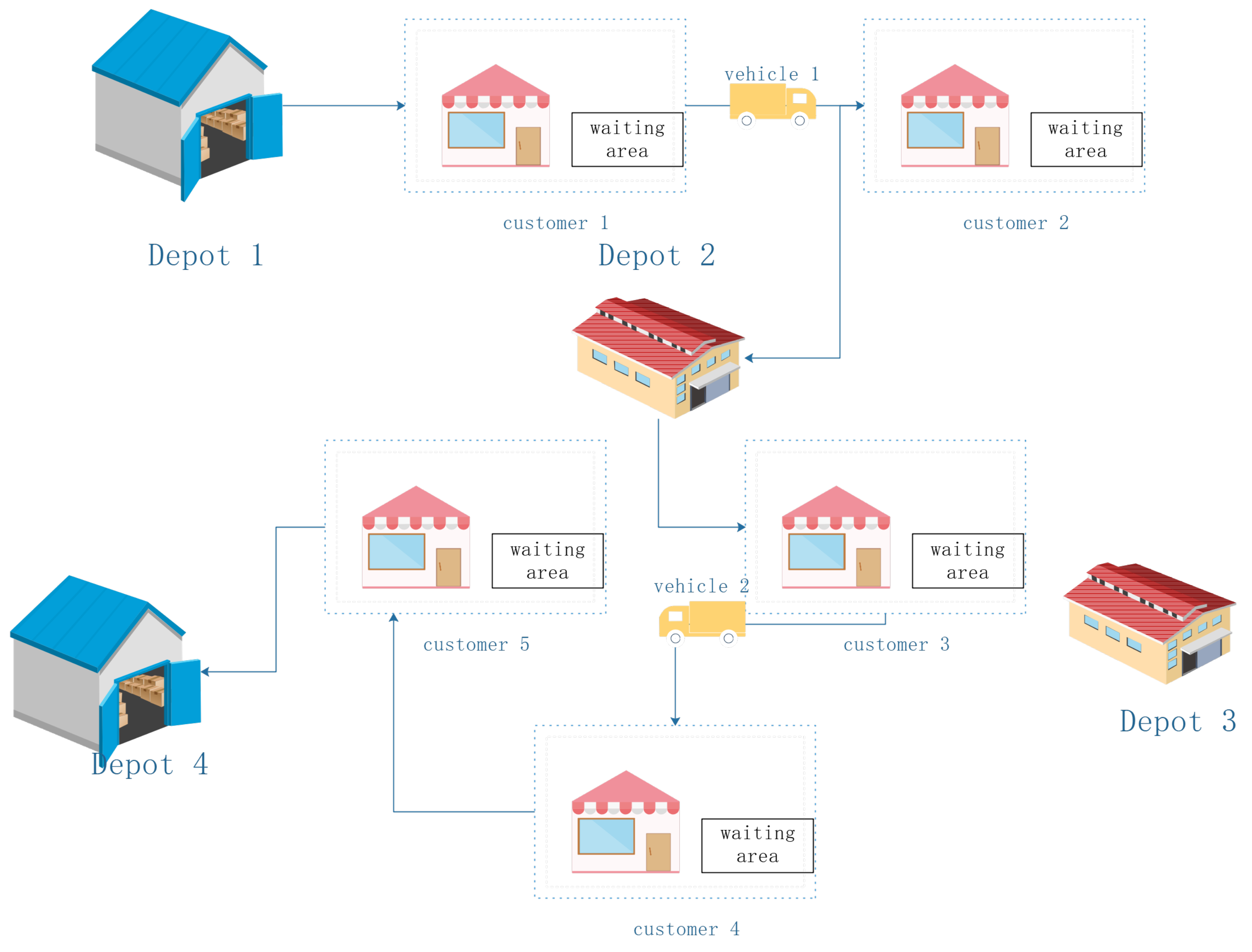
Figure 1. Example of distribution route results.
Symmetry 15 00124 g001
Figure 2. Dual-layer GA algorithm flow chart.
Symmetry 15 00124 g002
Figure 3. First case of temporal distance.
Symmetry 15 00124 g003
Figure 4. Second case of temporal distance.
Symmetry 15 00124 g004
Figure 5. Third case of temporal distance.
Symmetry 15 00124 g005
Figure 6. Last case of temporal distance.
Symmetry 15 00124 g006
Figure 7. Chromosome instance of the outer genetic algorithm, which has four paths and eight customer points.
Symmetry 15 00124 g007
Figure 8. Output results of an outer genetic algorithm with four paths and warehouse nodes added.
Symmetry 15 00124 g008
Figure 9. Genetic crossover example of the outer genetic algorithm, which contains eight customer nodes.
Symmetry 15 00124 g009
Figure 10. Example of exchange; there are eight customer points in one path.
Symmetry 15 00124 g010
Figure 11. Example of insert; there are eight customer points in one path.
Symmetry 15 00124 g011
Figure 12. Example of 2-opt; there are eight customer points in one path.
Symmetry 15 00124 g012
Figure 13. Inner genetic algorithm chromosome example; there are seven customer points in one path.
Symmetry 15 00124 g013
Figure 14. Crossover operator of the inner genetic algorithm, the chromosomes here have a dimension of 8, including eight waiting times.
Symmetry 15 00124 g014
Figure 15. Mutate operator of the inner genetic algorithm; the chromosomes here have a dimension of 8, including eight waiting times.
Symmetry 15 00124 g015
Figure 16. Time-varying speed function.
Symmetry 15 00124 g016
Figure 17. Fitness values of the inner genetic algorithm under different mutation rates.
Symmetry 15 00124 g017
Figure 18. Fitness values of the inner genetic algorithm under different crossover rates when the mutation rate is 0.2.
Symmetry 15 00124 g018
Figure 19. Fitness values of different population numbers under the condition of 0.2 mutation rate and 0.97 crossover rate of the inner genetic algorithm.
Symmetry 15 00124 g019
Figure 20. Fitness values of the outer layer genetic algorithm under different crossover rates with the inner layer genetic algorithm’s mutation rate of 0.2, crossover rate of 0.97, and population size of 50.
Symmetry 15 00124 g020
Figure 21. Average fitness values of the outer layer genetic algorithm’s crossover rate of 0.9 with the inner layer genetic algorithm’s mutation rate of 0.2, crossover rate of 0.97, and population size of 50.
Symmetry 15 00124 g021
Figure 22. Min fitness values of the outer layer genetic algorithm’s crossover rate of 0.9 with the inner layer genetic algorithm’s mutation rate of 0.2, crossover rate of 0.97, and population size of 50.
Symmetry 15 00124 g022
Figure 23. Max fitness values of the outer layer genetic algorithm’s crossover rate of 0.9 with the inner layer genetic algorithm’s mutation rate of 0.2, crossover rate of 0.97, and population size of 50.
Symmetry 15 00124 g023
Table 1. Parameter description.
ParametersDefinitions
DThe set of depots
CThe set of customers
VThe set of all nodes, The union of D and C
EThe edge set
Kthe set of all vehicles
QMaximum load capacity of the vehicle
WMaximum waitable time per node
[ T s , T f ] The time window of the depot
T s The earliest time the vehicle can leave the depot
T f The latest time a vehicle can arrive at the depot
[ E T i , L T i ] Time window for node i
d i j Distance between node i and node j, in km
d i Demand for node i
t i k d Time of departure of vehicle k at node i
t i k a Time of arrival of vehicle k at node i
t i k w Time of waiting of vehicle k at node i
t i s Service time required for node i
q i j k Load weight on the path from node i to node j on vehicle k
t i j travel time between node i and node j
c f u e l Cost per liter of fuel
c f i x e d Fixed cost per vehicle
c e Early arrival time window penalty for early arrival at the node
c l Late time window penalty for arriving at the node overtime
E i j Emissions of the vehicle from node i to node j
F i j Fuel consumption of the vehicle driving from node i to node j
x i j k If vehicle k drives from node i to node j, x i j k = 1 , else x i j k = 0
y i j If the customer i is served by the depot j, y i j = 1 , e l s e y i j = 0
Table 2. The dataset obtained by modifying the dataset P01.
Nodexy d i ET i LT i Nodexy d i ET i LT i
137520.158.09.02−49−490.212.513.0
3−52640.87.59.0420−260.758.518.0
540−300.5511.516.06−21470.7513.518.5
717630.710.018.5831−620.514.516.0
9−52330.657.513.01051210.9514.017.0
1142410.212.015.012−31−320.8513.513.0
13−5−250.113.514.51412−420.98.59.0
15−36−160.6511.013.51652−410.46.512.0
17−27−230.3513.514.51817−330.88.017.5
1913130.26.09.020−57580.68.018.0
2162−420.112.515.022−42570.0111.017.5
23−16−570.0511.513.024−8520.48.010.5
257−380.3511.513.026−27−680.714.017.0
2730480.312.517.528−43670.458.58.0
2958−480.89.011.030−58271.057.018.0
3137690.9510.013.03238460.613.514.5
33−46100.211.015.03461−331.010.012.0
3562630.610.515.536−63−690.6513.017.5
3732220.810.018.53845−350.2512.012.0
39−59150.913.513.5405−60.757.59.0
4110−170.3511.517.54221−100.359.512.5
43−5640.018.012.044−30150.66.016.0
4539−100.658.514.546−32390.758.516.5
47−25320.212.016.54825550.3510.515.0
49−48−280.111.014.05056370.6510.511.
D12020 6.018.D2−3040 6.018.0
D350−30 6.018.0D4−60−50 6.018.0
Disclaimer/Publisher’s Note: The statements, opinions and data contained in all publications are solely those of the individual author(s) and contributor(s) and not of MDPI and/or the editor(s). MDPI and/or the editor(s) disclaim responsibility for any injury to people or property resulting from any ideas, methods, instructions or products referred to in the content.