Article

Statistical Modelling for the Darcy–Forchheimer Flow of Casson Cobalt Ferrite-Water/Ethylene Glycol Nanofluid under Nonlinear Radiation

1
School of Mathematics and Statistics, Nanjing University of Information Science and Technology, Nanjing 210044, China
2
Department of Basic Sciences, College of Science and Theoretical Studies, Saudi Electronic University, Riyadh 11673, Saudi Arabia
3
Department of Statistics, Quaid-i-Azam University, Islamabad 45320, Pakistan
4
Department of Mathematics, Faculty of Science, Khon Kaen University, Khon Kaen 40002, Thailand
*
Author to whom correspondence should be addressed.
Symmetry 2022, 14(8), 1717; https://doi.org/10.3390/sym14081717
Submission received: 9 July 2022 / Revised: 3 August 2022 / Accepted: 9 August 2022 / Published: 17 August 2022
(This article belongs to the Special Issue Symmetry of Nanofluids and Their Applications in Engineering)

Abstract

:
Current research is focused on the utilization of a numerical solution of Casson cobalt ferrite nanofluid flow by taking two forms of base fluid. This investigation includes the gradual influence of nonlinear thermal radiation on the improvement of heat transfer related to the flow of nanofluids over a stretched rotating surface by the Darcy–Forchheimer law. The model constructed by a Casson nanoliquid in the boundary layer’s flow is studied for its symmetric behaviour, including cobalt ferrite nanomaterials. Two base liquids named as ethylene glycol and water are considered. The rate of heat transport is examined by considering Newtonian heating conditions. By utilizing similarity transformations, a partial differential system that governs the said model has been transformed into a highly nonlinear ordinary differential system, and numerical outcomes are obtained by implementing the RK4 via shooting methodologies. All obtained results, including local skin friction coefficients and local Nusselt number, are defined and discussed in the paper. The study’s findings ensure that the Casson cobalt ferrite nanofluid flowing towards a stretching plate has a unique solution: A variation of the solid volume fraction corresponds to the decrease in various values of the Casson nanofluid parameter for both type of nanofluid. Furthermore, a similar behaviour is noted for various values of the solid volume fraction, which corresponds to various values of the inertia coefficient parameter. Moreover, for the highest values of the solid volume fraction and all values of R 1 and N i taken into account, the rate of heat transfer upsurges. The data from the local skin friction coefficient (LSFC) and local Nusselt number (LNN) have been analysed using various statistical distributions, and it has been determined that both datasets generally fit the exponentiated Weibull distribution for various values of considered parameters. The findings would serve as a starting point for the manufacture of devices.

1. Introduction

There are extensive spectra of applications of flow and heat transfer along a stretching surface in numerous technological processes; polymer extrusion, including wire drawing; the manufacture of glass fiber; continuous casting; the manufacture of food and paper; plastic film’s stretching, etc. During the manufacture of these surfaces, melting occurs through a slit and is subsequently stretched to achieve the desired thickness. The final product’s required qualities are solely determined by the stretching rate, stretching procedure, and cooling rate during the process. Nevertheless, due to several uses of nanofluids flow, several investigators have been attracted by it, including nanofluid adhesives: transformer cooling, vehicle cooling, electronic devices cooling, electronics cooling, super powerful and small computer cooling; medical applications: safer surgery and cancer therapy by cooling and process industries; chemicals and materials: detergency, drink and food, paper, printing, and textiles. Several industrial technologies require intense and highly efficient cooling [1,2,3]. Traditional heat transfer fluids, such as thermic, water, and ethylene glycol, are widely used in a variety of industrial applications, including air conditioning and refrigeration, transportation, microelectronics, and solar thermal applications. However, the limitations in the performance of these heat transfer fluids require novel strategies for improving thermal transport properties and for increasing the energy efficiency of systems. It is generally known that suspending micro-solid particles in a base fluid produces a great heat transfer potential [4]. Despite this, the size of suspended pieces adds to precipitation, abrasion, and clogging in the fluid’s flow direction. The remarkable advancements in nanotechnology have resulted in the development of a revolutionary type of heat transmission liquid known as the nanofluid, which contains suspended pieces of less than 100 nm in size. Nanopowders such as Cu, Al, CuO, and SiC, as well as carbon nanotubes, are examples of nanomaterials (CNTs). The thermal conductivity of heat transport liquids has a substantial impact on increasing heat transfer rates, and many studies on the thermal conductivity of nanoliquids, particularly water- and ethylene glycol-based nanoliquids, have been conducted. In comparison to the base fluid, the experimental examinations of nanoliquid thermal conductivity revealed a considerable increase. Lee et al. [5] measured the thermal conductivity of several oxide nanoliquids (Al2O3 in ethylene glycol, Al2O3 in water, CuO in ethylene glycol, and CuO in water) and found that the ethylene glycol–CuO nanoliquid increased thermal conductivity by more than 20%. However, a 40% increase in thermal conductivity in ethylene glycol–Cu nanoliquid documented by Eastman et al. [6] resulted in an improvement. Xie et al. [7] explored the role of base liquids on the thermal conductivity of nanofluids using a variety of base fluids. With the increased thermal conductivity of the base fluid, the thermal conductivity ratio decreased. As a result, nanofluids could be an intriguing choice for enhanced heat-transport applications in the future, specifically those in the micro-scale. Furthermore, Dogonchi et al. [8] studied the significance of natural convective magnetic nanoliquids in an enclosure with a porous medium by taking Brownian motion phenomena. Shafiq et al. [9] analyzed the single as well as multiple wall carbon nanotubes on magnetohydrodynamic stagnant-point nanoliquid flow towards variable thick plates towards concave and convex phenomena. Hayat et al. [10] examined the Stratification impact on MHD Tangent hyperbolic nanofluid flow, which is induced by inclined surfaces. Shafiq et al. [11] investigated the Casson magnetohydrodynamic axisymmetric Marangoni forced-convection nanofluid flow towards a flat surface. Rehman et al. [12] analyzed the heat transport with nano-sized materials suspended in a magnetized rotatory flow field. Marangoni convective boundary-layer carbon-nanotube flow over a Riga surface was studied by Shafiq et al. [13]. Shafiq et al. [14] developed an artificial neural network (ANN) model to predict the flow of a single-walled carbon nanotube liquid over three various non-linear thin isothermal needles of cone, paraboloid, and cylinder shapes under convective conditions. The temperature profile increased according to the Biot number. Moreover, Shafiq et al. [15] studied hydromagnetic unsteady Williamson nanoliquid flows towards a radiative plate via numerical as well as artificial neural network modeling. They found good agreements according to the numerical results with ANN results. Noteworthy developments concerning nanoliquids can be found in refs. [16,17,18,19,20].
Porous media flows are particularly popular among engineers, mathematicians, and modelers due to its involvement in geothermal energy resources, oil reservoir modeling in isolation processes, crude oil processing, groundwater systems, water movement in reservoirs, etc. Heat transfer causes the flow in porous media to become even more important in processes involving thermal insulation materials, solar collectors and receivers, nuclear waste disposal, and energy storage systems [21,22,23]. Thus, much focus has been provided in the existing literature on certain porous media problems that are developed and produced using the classical Darcy theory. Under lower velocity and small porosity conditions, the classic Darcy principle remains true. When there are inertial and boundary impacts at a high flow rate, Darcy’s rule is insufficient. Nonlinear flow is caused when the Reynolds number is greater than unity. The effects of inertia and constraints cannot be neglected in some situations. Under these conditions, the effects of inertia and boundaries cannot be overlooked. To assess inertia and boundary effects, Forchheimer [24] added a square velocity equation to the Darcian velocity term. This word is known as the “Forchheimer term”, according to Muskat [25], and it is always true for large Reynolds numbers. In fact, in the momentum expression, larger filtration velocities result in quadratic drag for porous materials. In [26], the authors studied the effects of thermophoresis and viscous dissipation in Darcy–Forchheimer mixed convection flows embedded in porous medium. They considered two cases in which one corresponded to the presence of viscous dissipation and the other one corresponded to the absence of it. In [27], the authors implemented Darcy–Forchheimer law to examine the hydromagnetic flow of variate viscosity fluid in a porous medium. The most recent achievements for further Darcy–Forchheimer laws in different geometries and effects are discussed in refs. [28,29,30,31,32,33].
The goal of this research study, which was inspired by Jedi et al. [34], is to investigate the importance of the Darcy–Forchheimer flow of Casson cobalt ferrite nanofluids towards a rotating disk under Newtonian heating conditions statistically. Cobalt ferrite nanomaterials with water and ethylene glycol are considered. The porous space describing Darcy Forchheimer expression is filled by Casson fluids. The major goal here is to determine the influence of the critically considered variables. To solve a set of governing equations, the numerical shooting technique with the Runge–Kutta scheme is applied after similarity transformations. A physical–statistical model, as well as its distribution, was used to study the thermal conductivity of a Casson nanoliquid containing cobalt ferrite nanoparticles via two base fluids: water and ethylene glycol. The proposed model could also be employed in nanoliquid investigations for a wide range of practical commercial applications such as refrigeration and air conditioning, microelectronics, transportation, and solar thermal. Such an investigation is novel and unachieved, according to the finest complete evaluation to date.

2. Mathematical Modelling

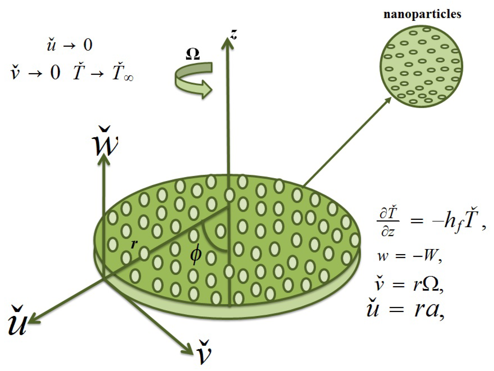
A steady Darcy–Forchheimer flow of Casson nanofluid flow towards a rotating disk is considered. The phenomenon of heat transfer is examined with nonlinear thermal radiation, Newtonian heating, and viscous dissipation. The porous space via DF expression is filled by an incompressible Casson cobalt ferrite nanoparticle liquid. The current investigation includes two kind of base fluids: One is water, and the other is ethylene glycol, while cobalt ferrite is taken as the nanomaterial. Furthermore, such nanomaterials are friendly and appropriate for soil microbes and in their involved processes. At z = 0, the disk spins with Ω as the constant angular velocity (see Figure 1). The governing equations according to above mentioned assumptions are as follows [18,20]:
u ˇ r + w ˇ z = u ˇ r ,
u ˇ u ˇ r + w ˇ u ˇ z v ˇ 2 r = 1 ρ n f p r + 1 + 1 γ 1 μ n f ρ n f 2 u ˇ r 2 u ˇ r 2 + 1 r u ˇ r + 2 u ˇ z 2 μ n f ρ n f u ˇ K * F * u 2 ,
u ˇ v ˇ r + u ˇ v ˇ r + w ˇ v ˇ z = 1 + 1 γ 1 μ n f ρ n f 2 v ˇ r 2 + 1 r v ˇ r v ˇ r 2 + 2 v ˇ z 2 μ n f ρ n f v ˇ K * F * v ˇ 2 ,
u ˇ w ˇ r + w ˇ w ˇ z = 1 ρ n f p z + 1 + 1 γ 1 μ n f ρ n f 2 w ˇ r 2 + 2 w ˇ z 2 + 1 r w ˇ r ,
w ˇ T ˇ z + u ˇ T ˇ r = 1 ρ c p n f k n f + 16 σ 1 * 3 k 1 * T 3 2 T ˇ r 2 + 1 r T ˇ r + 2 T ˇ z 2 + 16 σ 1 * 3 k 1 * T 2 T ˇ r 2 + T ˇ z 2 + 2 μ n f ρ c p n f 1 + 1 γ 1 u ˇ r 2 + u ˇ 2 r 2 + w ˇ z 2 + μ n f ρ c p n f 1 + 1 γ 1 v ˇ z 2 + w ˇ r + u ˇ z 2 + r r v ˇ r 2 ,
with
u ˇ = r a , v ˇ = r Ω , w ˇ = W , T ˇ z = h f T ˇ , at z = 0 ,
u ˇ 0 , v ˇ 0 , T ˇ T ˇ when z ,
where u ˇ = r a and v ˇ = r Ω are stretched velocity and rotational speed, respectively. The effective thermophysical characteristics of the nanofluids are provided below.
μ ˇ n f = μ f 1 α 2.5 , α ˇ n f = k ˇ n f ρ c p n f , ρ ˇ n f = 1 α ρ f + α ρ s , v ˇ n f = μ ˇ n f ρ ˇ n f , k ˇ n f k ˇ f = k s + 2 k f 2 α k f k s k s + 2 k f + α k f k s , ( ρ c p ) n f = ( 1 α ) ( ρ c p ) f + α ( ρ c p ) s .
The transformations into consideration are as follows.
u ˇ = r Ω f η , v ˇ = r Ω g η , w ˇ = 2 Ω ν f f η η = 2 Ω ν f 1 2 z , p = p Ω μ f P η , θ = T ˇ T ˇ T ˇ .
Utilizing the above-mentioned transformations and applying them in Equations (1)–(6), we obtain the following:
1 1 α 2.5 ( 1 α + α ρ s ρ f ) 1 + 1 β 1 2 f k 1 f + 2 f f f 2 + g 2 F r f 2 = 0 ,
1 1 α 2.5 ( 1 α + α ρ s ρ f ) 1 + 1 β 1 g k 1 g + 2 f g 2 f g F r g 2 = 0 ,
k n f k f 1 α + α ρ C p s ρ C p f 1 + 4 3 k f k n f R i 1 + θ f 1 θ 3 θ + Pr f θ + 6 Pr E c 1 α 2.5 f 2 + 4 R i 1 α + α ρ C p s ρ C p f 1 + θ f 1 θ 2 θ f 1 θ 2 + 2 Pr E c 1 α 2.5 1 + 1 β 1 f 2 + g 2 = 0 ,
f ( 0 ) = S 1 , f 0 = δ 1 , g 0 = 1 , θ ( 0 ) + N i ( 1 + θ ( 0 ) ) = 0 , f 0 , g ( ) 0 , θ ( ) 0 .
Here, the dimensionless parameters F r , k 1 , Pr , S 1 , R 1 , δ 1 , E c , and N i are presented as the inertia coefficient, the permeability parameter, the Prandtl number, the suction parameter, the radiation parameter, the stretching-strength parameter, the Eckert number, and the conjugate number, respectively, which are presented as follows.
F r = c d K * , k 1 = υ f Ω K * , Pr = υ f α f , S 1 = W 2 Ω υ f , R i = 4 σ 1 * T 3 k 1 * k f , E c = r 2 Ω 2 c p f k T , δ 1 = a Ω , N i = h f υ f 2 Ω .
Physical quantities, namely, the local skin friction coefficent (LSFC) and local Nusselt number (LNN), are defined in the following forms.
C f r = 2 τ r z ρ U w 2 , N u r = x q w K T ˇ T ˇ .
The dimensionless forms are as follows.
Re r 1 / 2 C f r = 1 1 ϕ 2.5 1 + 1 β 1 f 0 2 + g 0 2 ,
Re r 1 / 2 N u r = k n f k f + 4 3 R i 1 + θ f 1 θ 3 θ ( 0 ) .

3. Methodology

The shooting technique is employed to obtain the numerical simulation for (9)–(11) with boundary conditions (12). The shooting approach transforms a boundary-value problem (BVP) into an initial-value problem (IVP). Using the mathematically based RK4 scheme, the initial values of boundary value problems are obtained using the shooting technique and then numerically solved. For these numerical simulations, initial guesses are critical so that the initial conditions satisfy the solutions. After repeated iterations, the final convergent result was reached. As a general convergence criterion, a difference up to 10 5 is considered to be the upper limit. In this computational procedure, the substitutions f = y 1 , f = y 2 , f = y 3 , g = y 4 , y 4 = g = y 5 , θ = y 6 , and θ = y 7 are made to obtain the following.
y 1 = y 2 , y 2 = y 3 ,
y 3 = 1 2 k 1 y 3 + 1 α 2.5 ( 1 α + α ρ s ρ f ) 2 1 + 1 β 1 2 y 1 y 3 + y 2 2 y 4 2 + F r y 2 2 ,
y 5 = k 1 y 4 + 1 α 2.5 ( 1 α + α ρ s ρ f ) 1 + 1 β 1 2 f y 5 + 2 y 2 y 4 + F r y 4 2 ,
y 7 = 1 α + α ρ C p s ρ C p f k n f k f 1 + 4 3 k f k n f R i 1 + θ f 1 y 6 3 Pr y 1 y 7 6 Pr E c 1 α 2.5 y 2 2 4 R i 1 α + α ρ C p s ρ C p f 1 + θ f 1 y 6 2 θ f 1 y 7 2 2 Pr E c 1 α 2.5 1 + 1 β 1 y 3 2 + y 5 2 = 0 ,
y 1 ( 0 ) = S 1 , y 2 0 = δ 1 , y 4 0 = 1 , y 7 ( 0 ) + N i ( 1 + y 6 ( 0 ) ) = 0 , y 2 0 , y 4 ( ) 0 , y 6 ( ) 0 .

4. Model Selection and Discussion

The influences of β 1 , F r , N i , and R i on the LSFC and LNN were investigated. Table 1 lists the thermophysical properties of base fluids as well as nanomaterials. The different statistical models are mentioned in Table 2. Here, we illustrate the superiority of the suitably fitted model compared to some other distributions using three generated data sets for LSFC when β 1 = 0.1, 0.5, 0.9 and F r = 1.7, 2.1, 2.5, under water-cobalt ferrite (H2O-CoFe2O4), and ethylene glycol-cobalt ferrite (C2H6O2-CoFe2O4). Moreover, we generated another three datasets for LNN when R i = 0.1, 0.3, 0.6 and N i = 0.1, 0.2, 0.3 under water-cobalt ferrite (H2O-CoFe2O4), and ethylene glycol-cobalt ferrite (C2H6O2-CoFe2O4). For each data set, we estimate the model’s parameters by using maximum likelihood estimation from the above fitted models and listed them in Table 3, Table 4, Table 5 and Table 6. The following excellent statistical benchmarks have been used to compare these models: Anderson–Darling (A *), Cramer–von Mises (W *), and Kolmogorov–Smirnov (K-S) with p-values. The best model for the real data set might be the one with the lowest values of the above-mentioned goodness-of-fit (GoF) measures. These tests are used to determine the model’s goodness of fit and to identify which model best fits the data. The statistics A * and W * for each model are calculated using the algorithm in the R package [35], while the K-S is calculated using the algorithm in the R package GLDEX [36]. The statistics A * and W * were provided in detail by Chen and Balakrishnan [37]. The data are better represented by the model with the minimum value of these metrics and a large p-value (PV) than the other models. The values of goodness-of-fit (GOF) measures for the fitted models can be found in Table 7, Table 8, Table 9 and Table 10. Table 7 provides the values of GoF Statistics for the LSFC when β 1 = 0.1, 0.5, 0.9 under water-cobalt ferrite (H2O-CoFe2O4) and ethylene glycol-cobalt ferrite (C2H6O2-CoFe2O4). It is revealed from Table 7 that for the LSFC under water-cobalt ferrite (H2O-CoFe2O4), the EW model could be chosen as a best model among the other fitted models since it has the lowest values of the A * and W * and K-S statistics. It also has the largest PV of the KS test. For the LSFC of C2H6O2-CoFe2O4, three models could be chosen as the best model among the fitted models. As it can be seen, the results indicate that the Frechet model has the smallest values of Gof among the fitted models at β 1 = 0.1; therefore, it can be considered as the best model. It is noted that, the outcomes at β 1 = 0.5 indicates that the Weibull model has the smallest values of Gof among the fitted models. As a consequence, it may be called the best model. On the other hand, for the case of β 1 = 0.9, the EExF model has the smallest values of Gof among the fitted models; therefore, it can be considered as the best model.
Table 8 demonstrates that the EW model, which has the lowest values of the A * and W *, and K-S statistics is the best model among the fitted models for the LSFC of water-cobalt ferrite (H2O-CoFe2O4) at F r = 1.7, 2.1 and 2.5. The PV of the KS test is likewise the highest. Three different models could perhaps be considered as the best among the fitted models for the LSFC of C2H6O2-CoFe2O4, at F r = 1.7, 2.1 and 2.5 because the goodness-of-fit criterion is met by three models, namely, GHL, Weibull, and EW, at F r = 1.7, 2.1 and 2.5 respectively.
Table 9 shows that the EW model, with the exception of R i = 0.3, is the best model among the fitted models for the LNN of water-cobalt ferrite (H2O-CoFe2O4) and ethylene glycol-cobalt ferrite (C2H6O2-CoFe2O4) for R i = 0, 0.3 and 0.6. Whereas for R i = 0.3, the best model among the fitted models for the LNN of water-cobalt ferrite (H2O-CoFe2O4) is the Weibull model with the lowest values of the above-mentioned goodness-of fit (GoF) measures.
Table 10 reveals the following findings. For the LNN of water-cobalt ferrite (H2O-CoFe2O4), two models (Weibull and EW) could be chosen as the best model among the fitted models. At N i = 0.1, the Weibull model is the best since it has the lowest values of the above-mentioned goodness-of fit (GoF) measures; on the other hand, for N i = 0.2 and 0.3, Ew showed its suitability because of having the minimum values of GoF metrics. On the other hand, among the fitted models for the LNN of ethylene glycol-cobalt ferrite, the two models EW and EExF may be considered as the most appropriate ethylene glycol-cobalt ferrite (C2H6O2-CoFe2O4) for N i = 0.1 and N i = 0.2, 0.3, respectively, because the lowest values of GoF metrics for Ew and EExF demonstrated suitable suitability.
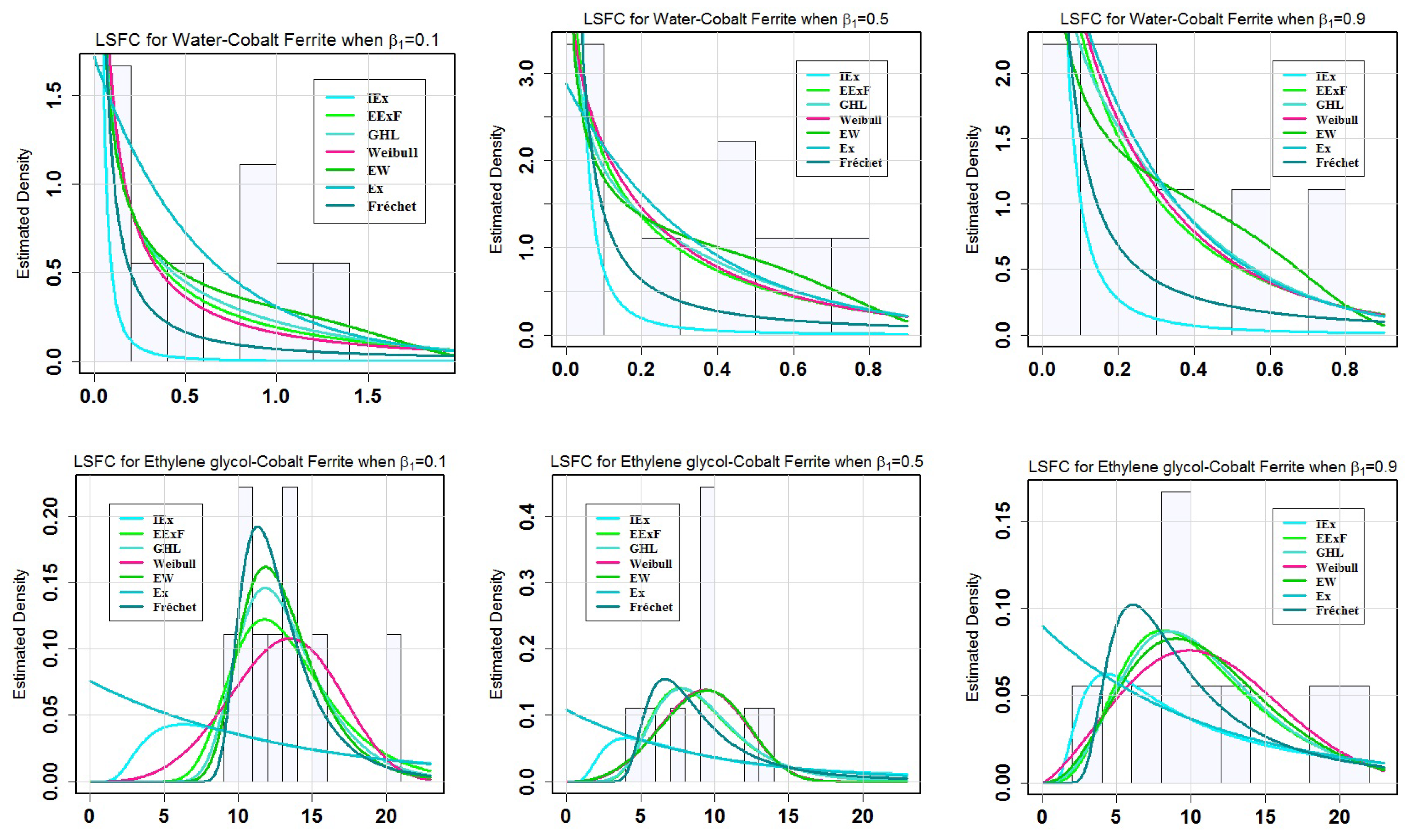
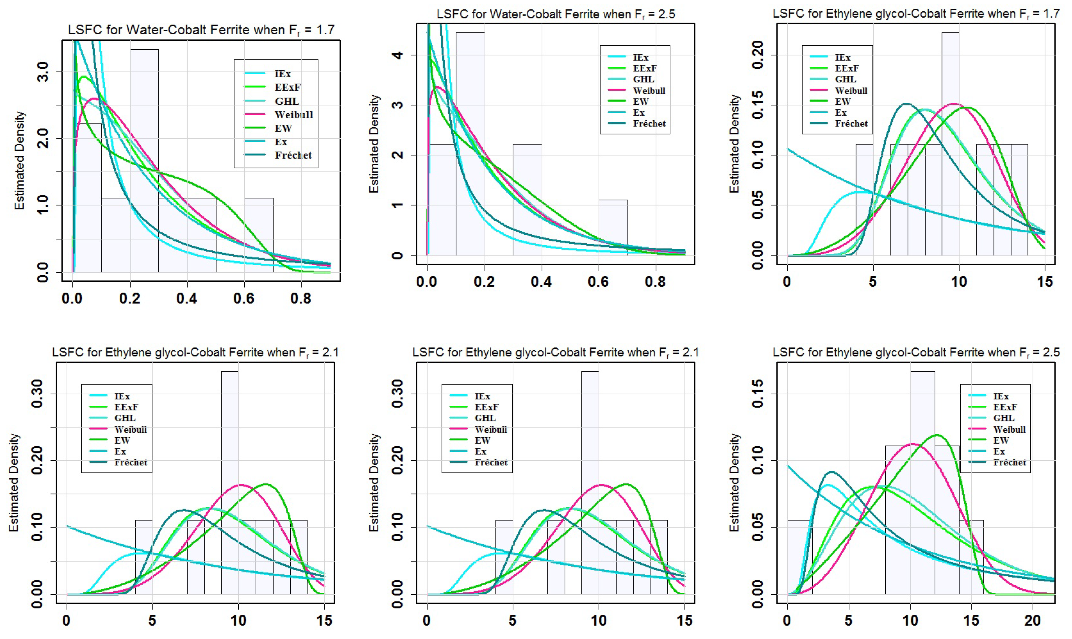
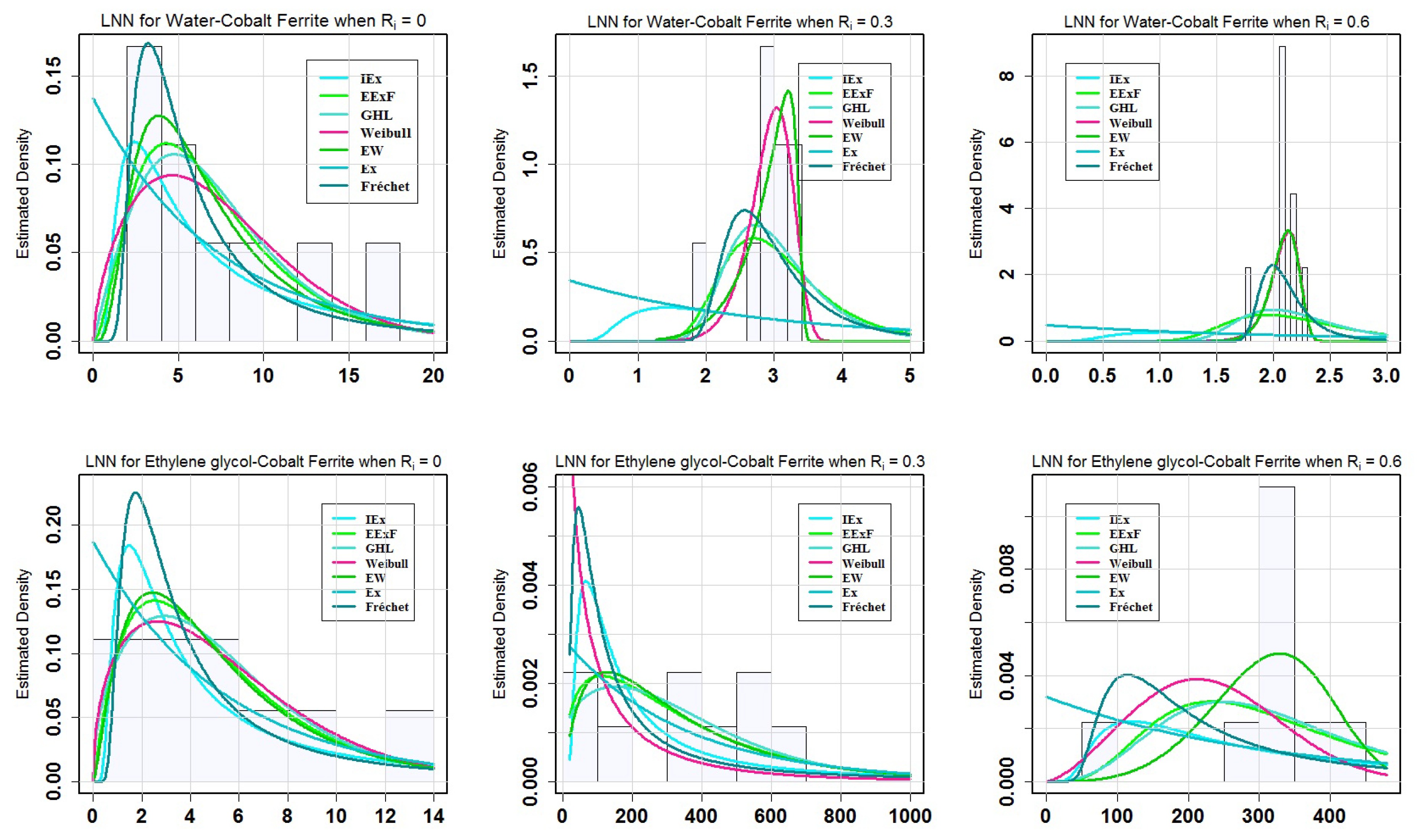
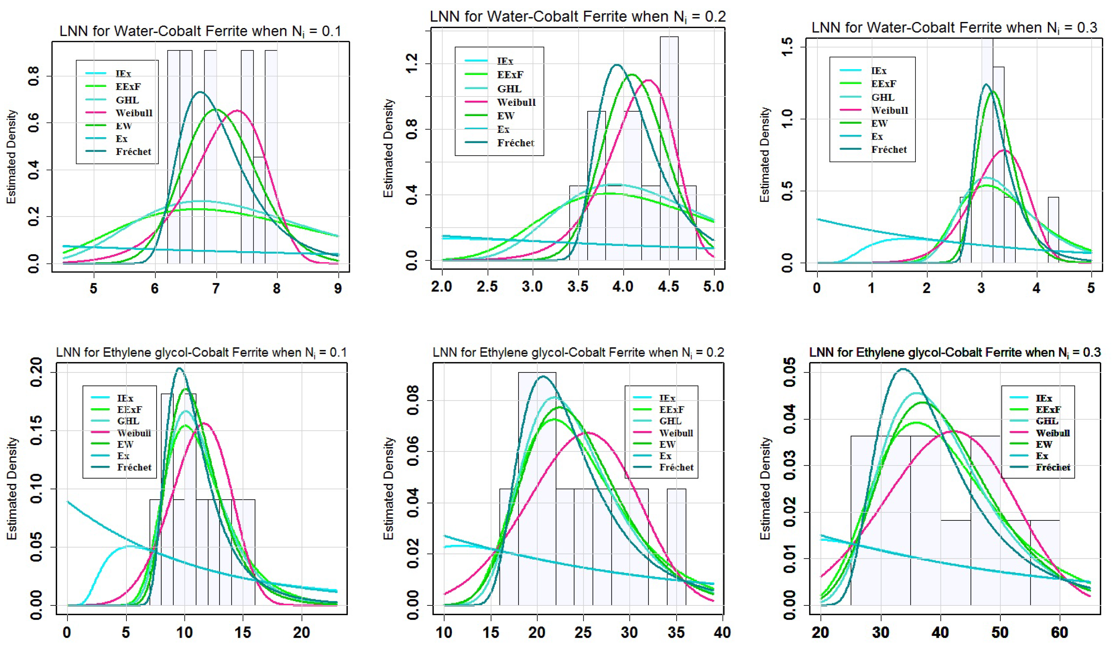
 Figure 2, Figure 3, Figure 4 and Figure 5 show the fitted models that support the findings of Table 7, Table 8, Table 9 and Table 10.
Figure 2, Figure 3, Figure 4 and Figure 5 show the fitted models that support the findings of Table 7, Table 8, Table 9 and Table 10. Figure 2 is plotted to observe the behaviour of the estimated models under water-cobalt ferrite (H2O-CoFe2O4), and ethylene glycol-cobalt ferrite (C2H6O2-CoFe2O4) at various levels of β 1 . From the upper panel of Figure 2, it is noted that the EW model is a suitable candidate for the data sets generated for water-cobalt ferrite (H2O-CoFe2O4) at all considered levels of β 1 . On the other hand, from the lower panel of Figure 2, the Frechet model showed good suitability with the data behavior generated for ethylene glycol-cobalt ferrite (C2H6O2-CoFe2O4) at β 1 = 0.1, whereas Weibull and EExF models provide the correct fit to the data generated at β 1 = 0.5, 0.9 compared to the other models. The behavior of estimated models under water-cobalt ferrite (H2O-CoFe2O4) and ethylene glycol-cobalt ferrite (C2H6O2-CoFe2O4) is plotted in Figure 3 at various levels of F r . It can be seen in the upper panel of Figure 3 that the EW model is a good fit for the data obtained for water-cobalt ferrite (H2O-CoFe2O4) at all values of F r . The GHL model, on the other hand, exhibited good appropriateness with the data behavior obtained for ethylene glycol-cobalt ferrite (C2H6O2-CoFe2O4) at F r = 1.7, besides the Weibull and EW models, when compared to the other models and provides the correct match to the data generated at F r = 2.1, 2.5. Figure 4 presents the characteristics of the estimated models for water-cobalt ferrite (H2O-CoFe2O4) and ethylene glycol-cobalt ferrite (C2H6O2-CoFe2O4) at different levels of R i . This is visible in the top panel of Figure 4 in which the EW model fits the data obtained for the water-cobalt ferrite (H2O-CoFe2O4) at R i = 0.1 and 0.6 values. The Weibull model, on the other hand, exhibited good appropriateness with the data at R i = 0.3. On the other hand, the EW model when compared to the other models, provided the best match for the data generated for ethylene glycol-cobalt ferrite (C2H6O2-CoFe2O4) at all values of R i . At varying quantities of N i , Figure 5 shows the pattern of estimated models for water-cobalt ferrite (H2O-CoFe2O4) (top panel) and ethylene glycol-cobalt ferrite (C2H6O2-CoFe2O4) (bottom panel). The EW model fits the data observed for the water-cobalt ferrite (H2O-CoFe2O4) for N i = 0.2 and 0.3, as shown in the top panel of Figure 5. At N i = 0.1, the Weibull model, on the other hand, showed good adequacy with the data. When compared to other models, the EW model provided the best fit to the data generated for the ethylene glycol-cobalt ferrite (C2H6O2-CoFe2O4 at N i = 0.1 and EExF model at N i = 0.2 and 0.3, respectively.

5. Concluding Remarks

The present investigation is focused on the utilization of a numerical solution of Casson cobalt ferrite nanofluid flow by taking two types of base fluid. The influence of nonlinear thermal radiation on the improvement in heat transfer corresponds to Darcy–Forchheimer Casson cobalt ferrite nanofluid flows over a stretched rotating surface and this phenomenon is investigated. Two base liquids named ethylene glycol and water were considered. The rate of heat transport is examined by considering the Newtonian heating condition. By utilizing similarity transformations, the governing differential system is solved numerically by implementing the RK4 via shooting techniques. The main findings are as follows:
  • For the LSFC under water-cobalt ferrite (H2O-CoFe2O4), the EW model can be chosen as the best model among the other fitted models at different levels of β 1 .
  • For the LSFC of ethylene glycol-cobalt ferrite (C2H6O2-CoFe2O4), three models, such as the Frechet, the Weibull, and EExF, can be chosen as the best models at β 1 = 0.1, 0.5, and 0.9, respectively.
  • The EW model, which has the lowest values of the A * and W * and K-S statistics, is the best model among the fitted models for the LSFC of water-cobalt ferrite (H2O-CoFe2O4) at F r = 1.7, 2.1 and 2.5.
  • For the LSFC under water-cobalt ferrite (H2O-CoFe2O4), the EW model can be chosen as a best model among the other fitted models since it has the lowest values of the A * and W * and K-S statistics and has the largest PV of the KS test.
  • For LNN, the EW model provided the best fit to the data generated for the ethylene glycol-cobalt ferrite (C2H6O2-CoFe2O4) at N i = 0.1 and EExF model at N i = 0.2 and 0.3, respectively

Author Contributions

A.S.: Conceptualization, Writing—review & editing, Data curation, Formal analysis, Methodology, Validation. S.A.L.: Formal analysis, Writing—original draft, Data curation, Methodology, Validation. T.N.S.: Conceptualization, Methodology, Writing—original draft, Data curation, Formal analysis, Validation, Conceptualization. K.N.: Supervision, Writing—review & editing. All authors have read and agreed to the published version of the manuscript.

Funding

This research received no external funding.

Data Availability Statement

All the data are available within the article.

Conflicts of Interest

The authors declare that they have no competing of interest.

Nomenclature

List of Symbols:
θ dimensionless temperature U w stretching velocity
h s heat transfer coefficient W·m−2·K−1fdimensionless velocity
μ ˇ n f nanofluid’s dynamic viscosity kg·m−1·s−1 ρ ˇ n f nanofluid’s density kg·m−3
μ ˇ n f nanofluid’s dynamic viscosity kg·m−1·s−1 c p specific heat
α nanomaterials solid volume fraction ρ p density of nanomaterials kg·m−3
k s nanomaterials thermal conductivity W·m−1·K−1 δ 1 stretching-strength parameter
k n f nanofluid’s thermal conductivity W·m−1·K−1 β 1 Casson fluid parameter
k f base fluid’s thermal conductivity W·m−1·K−1 F r Inertia coefficient
( ρ c p ) s nanoparticles heat S 1 suction parameter
capacitance J·kg2 m3·K−1 E c Eckert number
σ electrical conductivity of nanoliquidPrPrandtl number
τ the ratio of heat capacity of nanoparticles R 1 radiation parameter
by heat capacity of nanofluid N i Conjugate parameter
T ˇ temperature of liquid K Ω constant angular velocity
T ˇ ambient temperature K h f coefficient of heat transfer
K * permeability of porous medium F * = c b x K * non-uniform inertia
coefficient of porous medium
c b drag coefficient λ mixed convective number
u ˇ , v ˇ , w ˇ velocity components in r , φ , z directions k 1 permeability parameter
respectively ms−1

Abbreviations

LNNLocal Nusselt NumberEGethylene glycol
LSFCLocal Skin friction CoefficientIExInverse Exponential
GHLGeneralized Half LogisticDFDarcy–Forchheimer
EExFExponentiated Exponential FamilyExExponential
EWExponentiated Weibull

References

  1. Altan, T.; Oh, S.; Gegel, H. Metal Forming Fundamentals and Applications; American Society of Metals: Metals Park, OH, USA, 1979. [Google Scholar]
  2. Karwe, M.V.; Jaluria, Y. Numerical simulation of thermal transport associated with a continuous moving flat sheet in materials processing. ASME J. Heat Transf. 1991, 113, 612–619. [Google Scholar] [CrossRef]
  3. Kumaran, V.; Vanav Kumar, A.; Pop, I. Transition of MHD boundary layer flow past a stretching sheet. Commun. Nonlinear Sci. Numer. Simul. 2010, 15, 300–311. [Google Scholar] [CrossRef]
  4. Maxwell, J.C. A Treatise on Electricity and Magnetism, 2nd ed.; Clarendon Press: Oxford, UK, 1881. [Google Scholar]
  5. Lee, S.; Choi, S.U.S.; Li, S.; Eastman, J.A. Measuring thermal conductivity of fluids containing oxide nanoparticles. J. Heat Transf. 1999, 121, 280–289. [Google Scholar] [CrossRef]
  6. Eastman, J.A.; Choi, S.U.S.; Li, S.; Yu, W.; Thompson, L.J. Anomalously increased effective thermal conductivity of ethylene glycol based nanofluids containing copper nanoparticles. Appl. Phys. Lett. 2001, 78, 718–720. [Google Scholar] [CrossRef]
  7. Xie, H.; Lee, H.; Youn, W.; Choi, M. Nanofluids containing multiwalled carbon nanotubes and their enhanced thermal conductivities. J. Appl. Phys. 2003, 94, 4967–4971. [Google Scholar] [CrossRef]
  8. Dogonchi, A.S.; Seyyedi, S.M.; Hashemi-Tilehnoee, M.; Chamkha, A.J.; Ganji, D.D. Investigation of natural convection of magnetic nanofluid in an enclosure with a porous medium considering Brownian motion. Case Stud. Therm. Eng. 2019, 14, 100502. [Google Scholar] [CrossRef]
  9. Shafiq, A.; Khan, I.; Rasool, G.; Sherif, E.M.; Sheikh, A.H. Influence of Single-and Multi-Wall Carbon Nanotubes on Magnetohydrodynamic Stagnation Point Nanofluid Flow over Variable Thicker Surface with Concave and Convex Effects. Mathematics 2020, 8, 104. [Google Scholar] [CrossRef]
  10. Hayat, T.; Mumtaz, M.; Shafiq, A.; Alsaedi, A. Stratified MHD flow of Tangent hyperbolic nanofluid induced by inclined sheet. Appl. Math. Mech. 2017, 38, 271–288. [Google Scholar] [CrossRef]
  11. Shafiq, A.; Zari, I.; Rasool, G.; Tlili, I.; Khan, T.S. On the MHD Casson axisymmetric Marangoni forced convective flow of nanofluids. Mathematics 2019, 7, 1087. [Google Scholar] [CrossRef]
  12. Rehman, K.U.; Shahzadi, I.; Malik, M.Y.; Al-Mdallal, Q.M.; Zahri, M. On heat transfer in the presence of nano-sized particles suspended in a magnetized rotatory flow field. Case Stud. Therm. 2019, 14, 100457. [Google Scholar] [CrossRef]
  13. Shafiq, A.; Zari, I.; Khan, I.; Khan, T.S.; Seikh, A.H.; Sherif, E.S. Marangoni Driven Boundary Layer Flow of Carbon Nanotubes towards a Riga Plate. Front. Phys. 2020, 7, 215. [Google Scholar] [CrossRef]
  14. Shafiq, A.; Çolak, A.B.; Sindhu, T.N. Designing artificial neural network of nanoparticle diameter and solid–fluid interfacial layer on single-walled carbon nanotubes/ethylene glycol nanofluid flow on thin slendering needles. Int. Numer. Methods Fluids 2021, 93, 3384–3404. [Google Scholar] [CrossRef]
  15. Shafiq, A.; Çolak, A.B.; Sindhu, T.N.; Al-Mdallal, Q.M.; Abdeljawad, T. Estimation of unsteady hydromagnetic Williamson fluid flow in a radiative surface through numerical and artificial neural network modeling. Sci. Rep. 2021, 11, 14509. [Google Scholar] [CrossRef] [PubMed]
  16. Mirbagheri, M.H.; Akbari, M.; Mehmandoust, B. Proposing a new experimental correlation for thermal conductivity of nanofluids containing of functionalized multiwalled carbon nanotubes suspended in a binary base fluid. Int. Commun. Heat Mass Transf. 2018, 98, 216–222. [Google Scholar] [CrossRef]
  17. Abdullah, A.A.A.; Al-Rashed, A.; Shahsavar, A.; Akbari, M.; Toghraie, D.; Akbari, M.; Afrand, M. Finite Volume Simulation of mixed convection in an inclined lid-driven cavity filled with nanofluids: Effects of a hot elliptical centric cylinder, cavity angle and volume fraction of nanoparticles. Phys. A Stat. Mech. Appl. 2019, 527, 121122. [Google Scholar]
  18. Shafiq, A.; Sindhu, T.N.; Al-Mdallal, Q.M. A sensitivity study on carbon nanotubes significance in Darcy–Forchheimer flow towards a rotating disk by response surface methodology. Sci. Rep. 2021, 11, 1–26. [Google Scholar] [CrossRef]
  19. Esfe, M.H.; Afrand, M.; Wongwises, S.; Naderi, A.; Asadi, A.; Rostami, S.; Akbari, M. Applications of feedforward multilayer perceptron artificial neural networks and empirical correlation for prediction of thermal conductivity of Mg(OH)2–EG using experimental data. Int. Heat Mass Transf. 2015, 67, 46–50. [Google Scholar] [CrossRef]
  20. Shaw, S.; Dogonchi, A.S.; Nayak, M.K.; Makinde, O.D. Impact of Entropy Generation and Nonlinear Thermal Radiation on Darcy–Forchheimer Flow of MnFe2O4-Casson/Water Nanofluid due to a Rotating Disk: Application to Brain Dynamics. Arab. J. Sci. Eng. 2020, 45, 5471–5490. [Google Scholar] [CrossRef]
  21. Nield, D.A.; Bejan, A. Convection in Porous Media; Springer: New York, NY, USA, 1999. [Google Scholar]
  22. Karniadakis, G.; Beskok, A. Micro Flows; Springer: New York, NY, USA, 2002. [Google Scholar]
  23. Karniadakis, G.; Beskok, A.; Aluru, N. Micro Flows and Nano Flows: Fundamentals and Simulation; Springer: New York, NY, USA, 2005. [Google Scholar]
  24. Forchheimer, P. Wasserbewegung durch boden. Z. Ver. Dtsch. Ing. 1901, 45, 1782–1788. [Google Scholar]
  25. Muskat, M. The Flow of Homogeneous Fluids through Porous Media; J. W. Edwards: Ann Arbor, MI, USA, 1946. [Google Scholar]
  26. Seddeek, M.A. Influence of viscous dissipation and thermophoresis on Darcy-Forchheimer mixed convection in a fluid saturated porous media. J. Colloid Interface Sci. 2006, 293, 137–142. [Google Scholar] [CrossRef]
  27. Pal, D.; Mondal, H. Hydromagnetic convective diffusion of species in Darcy-Forchheimer porous medium with non-uniform heat source/sink and variable viscosity. Int. Commun. Heat Mass Transf. 2012, 39, 913–917. [Google Scholar] [CrossRef]
  28. Ramzan, M.; Shaheen, N. Thermally stratified Darcy–Forchheimer nanofluid flow comprising carbon nanotubes with effects of Cattaneo–Christov heat flux and homogeneous–heterogeneous reactions. Phys. Scr. 2019, 95, 015701. [Google Scholar] [CrossRef]
  29. Rasool, G.; Shafiq, A.; Khalique, C.M.; Zhang, T. Magnetohydrodynamic Darcy–Forchheimer nanofluid flow over a nonlinear stretching sheet. Phys. Scr. 2019, 94, 105221. [Google Scholar] [CrossRef]
  30. Rasool, G.; Zhang, T. Darcy-Forchheimer nanofluidic flow manifested with Cattaneo-Christov theory of heat and mass flux over non-linearly stretching surface. PLoS ONE 2019, 14, e0221302. [Google Scholar] [CrossRef] [PubMed]
  31. Dawar, A.; Shah, Z.; Islam, S.; Khan, W.; Idrees, M. An optimal analysis for Darcy–Forchheimer three-dimensional Williamson nanofluid flow over a stretching surface with convective conditions. Adv. Mech. 2019, 11, 1687814019833510. [Google Scholar] [CrossRef]
  32. Khan, U.; Ahmad, S.; Ramzan, M.; Suleman, M.; Lu, D.; Inam, S. Numerical Simulation of Darcy–Forchheimer 3D Unsteady Nanofluid Flow Comprising Carbon Nanotubes with Cattaneo–Christov Heat Flux and Velocity and Thermal Slip Conditions. Processes 2019, 7, 687. [Google Scholar]
  33. Do, Y.; Ramesh, G.K.; Roopa, G.S.; Sankar, M. Navier’s slip condition on time dependent Darcy-Forchheimer nanofluid using spectral relaxation method. J. Cent. South Univ. 2019, 26, 2000–2010. [Google Scholar] [CrossRef]
  34. Jedi, A.; Shamsudeen, A.; Razali, N.; Othman, H.; Zainuri, N.A.; Zulkarnain, N.; Bakar, N.A.; Pati, K.D.; Thanoon, T.Y. Statistical modeling for nanofluid flow: A stretching sheet with thermophysical property data. Colloids Interfaces 2020, 4, 3. [Google Scholar] [CrossRef]
  35. Gross, J.; Ligges, U. Package ‘nortest’. Five Omnibus Tests for Testing the Composite Hypothesis of Normality. 2015. Available online: https://cran.r-project.org/web/packages/nortest/index.html (accessed on 28 March 2019).
  36. Su, S.; GLDEX. Package: This Package Fits RS and FMKL Generalised Lambda. 2016. Available online: https://rdrr.io/cran/GLDEX/ (accessed on 28 March 2019).
  37. Chen, G.; Balakrishnan, N. A general purpose approximate goodness-of-fit test. J. Qual. Technol. 1995, 27, 154–161. [Google Scholar] [CrossRef]
Figure 1. Graphical layout and coordinate system.
Symmetry 14 01717 g001
Figure 2. The estimated densities for various values of β 1 under LSFC.
Symmetry 14 01717 g002
Figure 3. The estimated densities for various values of F r under LSFC.
Symmetry 14 01717 g003
Figure 4. The estimated densities for the LNN.
Symmetry 14 01717 g004
Figure 5. The estimated densities for the LNN.
Symmetry 14 01717 g005
Table 1. Thermophysical properties of base fluids and nanomaterials.
Base Fluid Physical Properties
ρ / kg · m 3 c p / ( J · kg 1 · K 1 ) k/ ( W · m 1 · K 1 ) Pr
(C2H6O2) Ethylene glycol (EG)111524300.253203.63
H2O (Water)997.141790.6136.2
Nanomaterial physical properties
CoFe2O4 (Cobalt ferrite)49077003.7-
Table 2. The distribution test for LSFC and LNN.
DistributionProbability Distribution Function g ( x )
IEx g ( x ; θ ˘ ) = θ ˘ x 2 exp ( θ ˘ x ) x > 0 , θ ˘ > 0 ,
where θ ˘ is regarded as the scale parameter
EExF g ( x ; η ^ , δ ^ ) = η ^ δ ^ ( 1 exp ( δ ^ x ) ) η ^ 1 exp ( δ ^ x ) x > 0 , η ^ , δ ^ > 0 ,
here η ^ is the shape parameter and δ ^ is the scale parameter.
GHL g ( x ; ζ ˘ , δ ^ ) = 2 ζ ˘ δ ^ exp ( δ ^ x ) ( 1 exp ( δ ^ x ) ) ζ ˘ 1 ( 1 + exp ( δ ^ x ) ) ζ ˘ + 1 x , ζ ˘ , δ ^ > 0 .
Where ζ ˘ is the shape parameter and δ ^ is the scale parameter.
Weibull g ( x ; γ ˘ , β ^ ) = β ^ γ ˘ ( x γ ˘ ) β ^ 1 e ( x γ ˘ ) β ^ x > 0 , γ ˘ , β ^ > 0 ,
where β ^ > 0 is the shape parameter and γ ˘ > 0 is the scale parameter.
EW g ( x ; α ˘ , β ˘ , ϑ ˘ ) = α ˘ β ˘ ϑ ˘ β ˘ x β ˘ 1 ( 1 exp ( ( ϑ ˘ x ) β ˘ ) ) α ˘ 1 exp ( ( ϑ ˘ x ) β ˘ ) x , α ˘ , β ˘ , ϑ ˘ > 0 ,
where α ˘ , β ˘ are shape parameters and ϑ ˘ is the scale parameter.
Ex g ( x ; σ ^ ) = σ ^ exp ( σ ^ x ) , x > 0 , σ ^ > 0 ,
where σ ^ is the scale parameter.
Fréchet g ( x ; ω ˘ , ϱ ˘ ) = ω ˘ x ( ϱ ˘ x ) ω ˘ e ( ϱ ˘ x ) ω ˘ x > 0 , α , ω ˘ > 0 ,
here ω ˘ is the shape parameter and ϱ ˘ is the scale parameter.
Table 3. Estimates of the parameters of statistical distribution for LSFC.
Re r 1 / 2 C fr
H2O-CoFe2O4C2H6O2-CoFe2O4
β1 = 0.1β1 = 0.5β1 = 0.9β1 = 0.1β1 = 0.5β1 = 0.9
IEx θ ˘ 0.004925720.00803380.0116116312.549118.2498538.687495
η ^ 0.37776650.68259080.760760148.133374117.47526175.8528827
EExF δ ^ 0.88385232.25937112.99891450.32900530.37232930.2168392
ζ ˘ 0.36284080.61914860.678199655.11423329.80255483.745755
GHL δ ^ 1.35147763.09327564.02557170.39735980.38153630.232938
γ ˘ 0.49710020.85887370.92370804.0972413.6958152.33285
Weibull β ^ 0.38655490.32865060.272327314.43626710.23040712.60927
α ˘ 0.14556370.13541670.123107558.075930938.38961692.2014263
EW β ˘ 2.51681364.54204604.78930461.24357050.81949371.5521847
ϑ ˘ 0.68131381.38882801.43612750.26095840.63437060.1139442
Ex σ ^ 0.58218860.34637853.5730920.075941890.10854520.08977783
Fréchet ω ˘ 0.021672720.04632130.046231111.6128757.3443897.652290
ϱ ˘ 0.342329820.39426540.43778275.9881542.9352941.881057
Table 4. Estimates of the parameters of statistical distribution for LSFC.
Re r 1 / 2 C fr
H2O-CoFe2O4C2H6O2-CoFe2O4
Fr = 1.7Fr = 2.1Fr = 2.5Fr = 1.7Fr = 2.1Fr = 2.5
IEx θ ˘ 0.0546940.0499820.0341840.04717128.801316.61957
η ^ 1.1740481.1595791.05928621.708049516.378023.70824
EExF δ ^ 4.0799074.1631694.6212080.38637250.339350.18816
ζ ˘ 0.9836940.9806450.89836612.0536109.393772.75686
GHL δ ^ 5.1235805.2719475.8824730.3948370.349310.21529
γ ˘ 1.2392911.2547541.1331894.1336964.647353.31257
Weibull β ^ 0.2865710.2787970.23309910.37472310.7216811.40295
α ˘ 0.1223390.1252790.3106320.458242590.207640.17935
EW β ˘ 6.3613226.4599262.5429516.8233088414.3700712.35625
ϑ ˘ 1.6609421.7998892.2945790.084428870.077780.07079
Ex σ ^ 3.7003693.8054394.4589320.1064220.102160.09638
Fréchet ω ˘ 0.0835460.0794800.0615727.6316697.800956.22488
ϱ ˘ 0.6543820.6381100.5977932.9901022.483811.14402
Table 5. Estimates of the parameters of statistical distribution for LNN.
Re r 1 / 2 Nu r
H2O-CoFe2O4C2H6O2-CoFe2O4
Ri = 0Ri = 0.3Ri = 0.6Ri = 0Ri = 0.3Ri = 0.6
IEx θ ˘ 4.799462.854490.139022.93598132.68050238.9850
η ^ 2.9430169.6795564.305662.057911.514255.70860
EExF δ ^ 0.250671.570152.1452850.285460.003750.00747
ζ ˘ 1.9847163.5809085.701601.476891.243053.79916
GHL δ ^ 0.274381.784482.577250.321090.004550.00807
γ ˘ 1.6439010.9668919.282941.453690.655332.49353
Weibull β ^ 8.202453.064792.141665.91572110.95909261.1334
α ˘ 12.004280.174091.2688122.834222.860820.87337
EW β ˘ 0.5914738.5599717.038250.857220.741474.78644
ϑ ˘ 1.016020.300780.472300.381720.006690.00283
Ex σ ^ 0.1372700.342750.479780.187340.002920.00320
Fréchet ω ˘ 4.259252.654832.005112.6914595.44180162.58202
ϱ ˘ 1.680325.2466812.405041.294710.945931.46931
Table 6. Estimates of the parameters of statistical distribution for LNN when δ 1 = δ 2 = δ 3 = 0.7 .
Re r 1 / 2 Nu r
H2O-CoFe2O4C2H6O2-CoFe2O4
Ni = 0.1Ni = 0.2Ni = 0.3Ni = 0.1Ni = 0.2Ni = 0.3
IEx θ ˘ 7.043874.106313.2467010.7248323.2919838.38786
η ^ 65.5349267.3674388.5708466.300111872.0393244.40364
EExF δ ^ 0.625871.095311.452710.41632720.195800.10546
ζ ˘ 66.4041766.9284871.3762048.738919661.8691943.62420
GHL δ ^ 0.723771.256151.609370.45343340.220580.12402
γ ˘ 13.0479812.806037.312295.0712244.778264.41743
Weibull β ^ 7.382824.301133.4716312.20211126.7403144.73431
α ˘ 15.6536812.1082730.823245.38378017.8226617.29216
EW β ˘ 4.182844.536422.85223124.65658211.539651.44738
ϑ ˘ 0.186180.306580.490221.04995190.090880.05712
Ex σ ^ 0.140910.241720.304230.44470170.040830.02451
Fréchet ω ˘ 6.7743693.949313.105669.87990221.3852335.16524
ϱ ˘ 13.4364912.7680410.425705.3837805.098624.75391
Table 7. Goodness-of-Fits Statistics for the LSFC.
Re r 1 / 2 C fr
H2O-CoFe2O4C2H6O2-CoFe2O4
β1 = 0.1β1 = 0.5β1 = 0.9β1 = 0.1β1 = 0.5β1 = 0.9
IExW *0.260590.303310.304210.035250.092330.05789
A *1.504751.748731.722600.275080.569910.40980
K-S0.654110.697330.714740.455310.446860.34439
PV0.000276.6 × 10−53.6 × 10−50.031810.037140.18630
EExFW *0.157310.090700.086640.035280.079320.04200
A *0.998650.571010.494750.275370.497400.27055
K-S0.294350.269680.289210.169300.211400.16701
PV0.346200.452100.366800.922400.742100.92940
GHLW *0.140850.076790.068550.032580.076460.04202
A *0.911460.485090.391690.252640.481880.27061
K-S0.277900.260670.262980.157060.206580.17693
PV0.415000.494600.483500.955300.766200.89670
WeibullW *0.184020.096560.091110.087530.051590.05599
A *1.136470.607440.520360.627450.330210.32478
K-S0.300340.262700.269290.200700.189830.21735
PV0.323100.484900.453900.795000.845000.71200
EWW *0.116640.047390.056580.031720.051750.04601
A *0.770640.308260.312380.245210.329750.28155
K-S0.261590.251750.227630.163380.195480.19333
PV0.490200.538200.660100.939700.819600.82940
ExW *0.156490.091260.087170.049410.064180.04409
A *0.995110.573800.497820.381900.409720.27689
K-S0.329870.255940.248990.521330.415420.35322
PV0.225400.517600.552000.008410.063980.16510
FréchetW *0.245650.224720.242430.025490.127140.08116
A *1.440501.362321.391320.176540.758490.56017
K-S0.356220.286190.352550.140450.250320.20570
PV0.158400.379300.166700.983200.545300.77060
Table 8. Goodness-of-fit statistics for the LSFC.
Re r 1 / 2 C fr
H2O-CoFe2O4C2H6O2-CoFe2O4
Fr = 1.7Fr = 2.1Fr = 2.5Fr = 1.7Fr = 2.1Fr = 2.5
IExW *0.221990.241260.249800.047170.143820.36806
A *1.311781.392961.448210.359470.908852.02909
K-S0.466080.527720.571700.478120.485000.36469
PV0.025990.007300.002600.020590.017970.14040
EExFW *0.066450.078530.069260.039680.115220.24185
A *0.396730.471700.405340.309530.746721.42151
K-S0.248970.240790.253250.139930.278340.31886
PV0.552000.593200.530800.983800.413000.25880
GHLW *0.051850.060220.055670.037880.108080.21581
A *0.309230.369170.326510.297140.705091.29001
K-S0.227200.213200.226720.135030.270290.30256
PV0.662200.733000.66470.988700.449300.31480
WeibullW *0.0580790.067750.064750.029600.049830.13728
A *0.3460250.410650.378610.211250.334710.86829
K-S0.226480.202140.228000.155060.194360.25317
PV0.665900.788000.658200.959700.824800.53120
EWW *0.039740.039170.051830.036650.054210.07977
A *0.235810.233910.305570.235050.325190.50882
K-S0.162180.168010.199940.164180.168400.24120
PV0.942800.926400.798600.937500.925200.59110
ExW *0.065890.077930.069110.030420.088410.22554
A *0.393370.468260.404450.243130.587431.33893
K-S0.261720.261440.261180.397930.437720.44141
PV0.489600.490900.492200.084920.043710.04095
FréchetW *0.189830.209770.207140.078270.197440.37788
A *1.133091.216571.216140.552841.1968272.07480
K-S0.275920.322650.331180.190540.309500.37796
PV0.423800.246900.221700.841900.29000.11550
Table 9. Goodness-of-fit statistics for the LNN.
Re r 1 / 2 Nu r
H2O-CoFe2O4C2H6O2-CoFe2O4
R1 = 0R1 = 0.3R1 = 0.6R1 = 0R1 = 0.3R1 = 0.6
IExW *0.015150.18130.137560.028690.190410.38233
A *0.131261.105290.817000.225411.085132.09143
K-S0.243180.574700.594880.198040.373530.44431
PV0.581200.002410.001440.807600.123400.03888
EExFW *0.019790.186110.139020.012550.142090.29568
A *0.152191.130600.825420.109250.793181.68073
K-S0.123970.308860.373640.094440.328210.36948
PV0.995700.292200.123200.999800.23020.13100
GHLW *0.024570.193870.143700.016030.148410.27457
A *0.181811.171110.852140.129760.827511.57840
K-S0.136030.288560.369170.107810.327410.34997
PV0.987800.36950.131600.999500.232600.17270
WeibullW *0.029650.076880.094550.016770.146590.20054
A *0.214050.508100.558090.134200.817581.20425
K-S0.131890.169840.235970.106630.561270.59595
PV0.991200.920700.617700.999600.003360.00140
EWW *0.014830.084540.093490.011780.132910.16038
A *0.122600.507440.552950.105350.744790.98821
K-S0.100060.201900.234300.093530.310610.23122
PV0.999900.789200.618101.000000.286100.64190
ExW *0.022060.149310.127210.013190.140640.27278
A *0.166300.934180.757140.112740.785371.56886
K-S0.244020.501100.572180.166010.338680.48518
PV0.576900.012940.002570.93230.201000.01790
FréchetW *0.019460.260360.216630.03550.187270.40106
A *0.164661.5069041.250460.27001.065002.17841
K-S0.111540.333880.354550.125460.430810.53184
PV0.999000.214000.162100.995000.049320.00666
Table 10. Goodness-of-fit statistics for the LNN.
Re r 1 / 2 Nu r
H2O-CoFe2O4C2H6O2-CoFe2O4
Ni = 0.1Ni = 0.2Ni = 0.3Ni = 0.1Ni = 0.2Ni = 0.3
IExW *0.075530.033130.233060.020210.020210.02020
A *0.492810.219021.223880.162200.162170.16210
K-S0.585870.577650.525210.497540.488980.47613
PV0.000400.000520.002360.004860.006010.00820
EExFW *0.075420.033220.229730.020180.020130.02014
A *0.492720.219801.204770.162070.161520.16299
K-S0.357690.306460.343230.093300.089860.08841
PV0.091450.205300.116400.999800.999900.99990
GHLW *0.075160.033370.227800.020210.020130.02016
A *0.492280.221191.193680.162230.161690.16366
K-S0.335660.286100.328230.090010.104880.10476
PV0.131600.272900.147900.999900.998500.99850
WeibullW *0.072770.041380.317090.037470.038140.03928
A *0.495250.275031.718510.267620.271720.27863
K-S0.190980.178170.325420.128780.129260.13003
PV0.750800.81740.154500.982200.981500.98050
EWW *0.076090.033270.229310.020140.020960.02118
A *0.495480.219171.202940.161690.166910.16826
K-S0.205520.142440.279820.105290.103670.10806
PV0.66980.954500.296600.998400.998700.99770
ExW *0.076570.033060.247890.0229090.023310.02399
A *0.495330.217191.311130.1788120.181270.18537
K-S0.589280.579840.556960.508720.501720.49199
PV0.000360.000490.000970.003650.004370.00558
FréchetW *0.072120.044730.225130.025040.024640.02400
A *0.493320.296601.184780.191550.189120.18512
K-S0.224690.143720.302810.114110.113850.11332
PV0.561300.953100.216400.995300.995400.99570
Publisher’s Note: MDPI stays neutral with regard to jurisdictional claims in published maps and institutional affiliations.

