Multi-Label Attribute Reduction Based on Neighborhood Multi-Target Rough Sets

Abstract

The rough set model has two symmetry approximations called upper approximation and lower approximation, which correspond to a concept’s intension and extension, respectively. Multi-label learning enforces the rough set model, which wants to be applied considering the correlations among labels, while the target concept should not be limited to only one. This paper proposes a multi-target model considering label correlation (Neighborhood Multi-Target Rough Sets, NMTRS) and proposes an attribute reduction approach based on NMTRS. First, some definitions of NMTRS are introduced. Second, some properties of NMTRS are discussed. Third, some discussion about the attribute significance measure is given. Fourth, the attribute reduction approaches based on NMTRS are proposed. Finally, the efficiency and validity of the designed algorithms are verified by experiments. The experiments show that our algorithm shows considerable performance when compared to state-of-the-art approaches.

1. Introduction

Since rough set theory was proposed by Pawlak [1] in 1982, it quickly became a hot topic in knowledge discovery and has been widely used in many applications such as classification [2,3,4,5,6], clustering [7,8,9,10,11], and attribute reduction [12]. It has two approximations corresponding to a target concept’s intension and extension, which shows symmetry. Various rough set models are based on different types of binary relations, such as multiple equivalence relations [13], general binary relations [14], and so on. Within these models, the neighborhood relation is outstanding for its ability to deal with both nominal and numerical attributes at the same time.

There are lots of works applying the neighborhood rough set model in various fields. Inbarani et al. [15] proposed a classification algorithm by using the neighborhood rough set model. For dynamic data mining, Zhang et al. [16] proposed a neighborhood rough set approach. Most relevant works applied the neighborhood rough set model to attribute reduction tasks.

Attribute reduction, or feature selection, is a traditional but essential machine learning task. Attribute reduction approaches try to select some features from the raw attribute set without harming the data’s information presentation ability. These approaches have made remarkable achievements in eliminating noise and promoting learning time efficiency. For attribute reduction tasks, there are different types of work. The first type is single-label attribute reduction. Hu et al. [17] proposed an approach for attribute reduction based on neighborhood rough sets. A quick attribute reduction algorithm was proposed by Yong et al. [18] based on the neighborhood rough set model. Additionally, there are parallel attribute reduction approaches [19], online streaming attribute reduction [20], and so on. These attribute reduction approaches were proposed based on the classic or extended neighborhood rough set model.

The second type of attribute reduction task is multi-label attribute reduction. These methods use strategies to handle the multiple labels in a multi-label learning paradigm. For example, Sun et al. [21] proposed a multi-label attribute reduction approach by transforming the multi-label learning problem into a single label one by ignoring the correlations within labels. Fisher R.A. et al. [22] regard the feature space and the label space as two different viewpoints of the data to improve the original dimension reduction method. By using the kernel matrix method, Wold H. et al. [23] proposed a similar method to [22]. By using the mapping dimensionality reduction and sub-control dimensionality reduction approaches at the same time, Zhang et al. [24] proposed a dimensionality reduction with a linear kernel matrix or non-linear kernel matrix. Based on PCA and genetic algorithms, Zhang et al. [25] proposed MLNB by using the Naive Bayes method to extract the features simultaneously. Liu et al. [26] proposed an attribute reduction method based on a neighborhood rough set model. Meanwhile, an online multi-label attribute reduction method was proposed by Liu et al. [27] using the neighborhood rough set model. The f-neighborhood rough set model was used to derive the feature selection method for multi-label learning [28].

The attribute reduction methods designed for single-label learning or multi-label learning based on neighborhood rough sets all use the classic neighborhood rough set model and its extended models. All of these neighborhood rough set models are designed for a classic information system [29,30,31,32,33,34,35], which means that the system only has one decision attribute. None of them are designed for a multi-decision information system that considers label correlation among labels simultaneously.

In this paper, we propose a neighborhood multi-target rough set model and then design an attribute reduction algorithm based on it. We design the model by defining a global correlated target set to be the target group of the rough set model. The coefficient of the global correlated target set controls the relevance of different target concepts. Then, we use a conservative strategy to combine the correlated target to define the rough set model. Using the rough set model which we proposed, the attribute significance measure can be then given. Furthermore, we can derive the corresponding attribute reduction algorithm.

The contributions of this paper are as follows:

• A neighborhood rough set model considering the label correlation is proposed for multi-label learning.
• The properties of the proposed models are investigated.
• An algorithm for calculating the approximations in the proposed rough set model is designed.
• Attribute significance measure is given based on the rough set model we proposed.
• Experiments are conducted to validate the efficiency and effectiveness of the proposed algorithms.

The rest of this paper is organized as follows. Some basic concepts of NMTRS are introduced, and their properties are discussed in Section 2. In Section 3, the attribute significance measure is given, along with some discussions about it, and the corresponding attribute reduction algorithms are derived by the significance measure. All the algorithms are evaluated in Section 4. Finally, we conclude the whole paper in Section 5.

2. Neighborhood Multi-Target Rough Sets

In this section, some concepts associated with our proposed model are introduced and then the properties of the proposed model are discussed.

2.1. Definitions

In this subsection, the definitions of neighborhood multi-target rough sets are introduced.

Definition 1.

[1] Suppose$U$is a finite universe and$A=\{a_1,a_2,\cdots ,a_m\}$is an attribute set, then$\left(U,A\right)$is an information system.

Definition 2.

[35] (Set Correlation, SC) Suppose$U$is a finite universe and$\left(U,A\right)$is an information system,$\mathit{X}=\left\{X_1,X_2,\cdots ,X_r\right\}$is a finite target set which satisfies for all$X_i\in \mathit{X},X_i\subseteq U$. The set correlation is defined by:

$$S_R\left(X_i,x_j\right)=|X_i\cap X_j|/\left|X_i\right|,i,j\le r (Relative Correlation) or$$

$$S_R\left(X_i,x_j\right)=|X_i\cap X_j|/|X_i\cup X_j|,i,j\le r (Absolute Correlation).$$

Definition 3.

(Global Correlated Target Set, GCTS) Suppose$U$is a finite universe and$\left(U,A\right)$is an information system,$\mathit{X}=\left\{X_1,X_2,\cdots ,X_r\right\}$is a finite target set which satisfies for all$X_i\in \mathit{X},X_i\subseteq U$. Then,$\mathit{X}$is a global correlated target set if and only if for all$X_i,X_j\in \mathit{X}$, $S_R(X_i,X_j)>\alpha$or$S_R(X_j,X_i)>\alpha$, $\alpha \in (0,1]$is the Correlation Control Parameter (CCP) among targets; it controls the relevance degree among targets in the target group.

Based on the definition of GCTS and neighborhood rough sets, we can define neighborhood multi-target rough sets accordingly.

Definition 4.

[34] (Neighborhood Class)Suppose$U$is a finite universe and$(U,A)$is an information system, where$A=A_C\cup A_N$,$A_C$is the symbol attribute set and$A_N$is the numerical attribute set. For all$x\in U,\delta \ge 0$, the neighborhood class of$x$can be defined as

$$\begin{array}{c}\left(1\right) n_{A_C}\left(x\right)=\left\{y\in U|\forall a\in A_C,y_a=x_a\right\};\hfill \\ \left(2\right) n_{A_N}\left(x\right)=\left\{y\in U\left|d\right(x_{A_N},y_{A_N})\le \delta \right\};\hfill \\ \left(3\right) n_A\left(x\right)=n_{A_C\cup A_N}\left(x\right)=\left\{y\in U|\forall a\in A_C,y_a=x_a\wedge d(x_{A_N},y_{A_N})\le \delta \right\}.\hfill \end{array}$$

where$y_a$denotes the attribute value of instance$y$on attribute$a$and where$y_{A_N}$denotes the attribute value of instance$y$on attribute set$A_N$.

Definition 5.

(Neighborhood Multi-Target Rough Sets, NMTRS) Suppose$U$is a finite universe and$\left(U,A\right)$is an information system,$\mathit{X}=\left\{X_1,X_2,\cdots ,X_r\right\}$is a finite target set which satisfies for all$X_i\in \mathit{X},X_i\subseteq U$. $\mathit{X}$is a GCTS and the correlation coefficient is$\alpha$.

Then, the lower approximation of NMTRS is defined as:

$${\underset{\_}{R}}_{\delta }^{\alpha }\left(\mathit{X}\right)=\left\{x\in U|n_A\left(x\right)\subseteq X_1\wedge n_A\left(x\right)\subseteq X_2\wedge \cdots \wedge n_A\left(x\right)\subseteq X_r\right\}.$$

The upper approximation of NMTRS is defined as:

$${\overline{R}}_{\delta }^{\alpha }\left(\mathit{X}\right)=\left\{x\in U|n_A\left(x\right)\cap X_1\ne \varphi \vee n_A\left(x\right)\cap X_2\ne \varphi \vee \cdots \vee n_A\left(x\right)\cap X_r\ne \varphi \right\}.$$

With the help of CCP, we can organize different targets together. The lower approximation is a conservative approximation of the target group and needs all the targets to meet the same condition. Relatively, the upper approximation obeys a liberal strategy and only needs one target of the target group to meet the condition.

Example 1.

A multi-label decision information system is as

Table 1. An information system.

$\mathit{x}$	${\mathit{n}}_1$	${\mathit{a}}_1$	${\mathit{a}}_2$	${\mathit{X}}_1$	${\mathit{X}}_2$
$x_1$	1.5	M	1	0	1
$x_2$	2	F	2	1	1
$x_3$	2	M	2	1	0
$x_4$	1.5	M	2	0	0
$x_5$	2	F	2	1	1

below: it has two labels which are assumed to be two different target concepts. We can easily obtain that when α = 0.4 the target group is a GCTS. For clarifying the definition of NMTRS, we have an example for NMTRS. Since

$$X_1=\left\{x_2,x_3,x_5\right\},X_2=\left\{x_1,x_2,x_5\right\},\alpha =0.4,\delta =0.5,S_R\left(X_1,X_2\right)=2/3>\alpha =0.4.$$

From Table 1 we have

$$n_A\left(x_1\right)=\left\{x_1\right\},n_A\left(x_2\right)=\left\{x_2,x_5\right\},n_A\left(x_3\right)=\left\{x_3,x_4\right\},n_A\left(x_4\right)=\left\{x_3,x_4\right\},n_A\left(x_5\right)=\left\{x_2,x_5\right\}.$$

From Definition 5,

$$\begin{array}{c}{n}_A\left(x_1\right)=\left\{x_1\right\} \not\subset X_1\wedge n_A\left(x_1\right)\subseteq X_2,n_A\left(x_2\right)\subseteq X_1\wedge n_A\left(x_2\right)\subseteq X_2,n_A\left(x_3\right) \not\subset X_1\wedge n_A\left(x_3\right) \not\subset X_2,\hfill \\ n_A\left(x_4\right) \not\subset X_1\wedge n_A\left(x_4\right) \not\subset X_2,n_A\left(x_5\right)\subseteq X_1\wedge n_A\left(x_5\right)\subseteq X_2,\hfill \\ \therefore {\underset{\_}{R}}_{\delta }^{\alpha }\left(\mathit{X}\right)=\left\{x_2,x_5\right\}.\hfill \end{array}$$

$$\begin{array}{c}{n}_A\left(x_1\right)\cap X_2\ne \varphi ,n_A\left(x_2\right)\cap X_1\ne \varphi ,n_A\left(x_3\right)\cap X_1\ne \varphi ,n_A\left(x_4\right)\cap X_1\ne \varphi ,n_A\left(x_5\right)\cap X_1\ne \varphi ,\hfill \\ \therefore {\overline{R}}_{\delta }^{\alpha }\left(\mathit{X}\right)=U. \hfill \end{array}$$

2.2. Properties

The properties of NMTRS are discussed in this subsection.

Proposition 1.

Suppose$U$is a finite universe and$\left(U,A\right)$is an information system,$\mathit{X}=\left\{X_1,X_2,\cdots ,X_r\right\}$is a finite target set which satisfies for all$X_i\in \mathit{X},X_i\subseteq U$. $\mathit{X}$is a GCTS and the correlation coefficient is$\alpha$. For the approximations of NMTRS:

$$\begin{array}{l}\left(1\right) for all X_i\in \mathit{X},X_i=U if and only if {\underset{\_}{R}}_{\delta }^{\alpha }\left(\mathit{X}\right)=U;\\ \left(2\right) exists X_i\in \mathit{X},X_i=U if and only if {\overline{R}}_{\delta }^{\alpha }\left(\mathit{X}\right)=U;\hfill \\ \left(3\right) exists X_i\in \mathit{X},X_i=\varphi if and only if {\underset{\_}{R}}_{\delta }^{\alpha }\left(\mathit{X}\right)=\varphi ;\hfill \\ \left(4\right) for all X_i\in \mathit{X},X_i=\varphi if and only if {\overline{R}}_{\delta }^{\alpha }\left(\mathit{X}\right)=\varphi ;\hfill \\ \left(5\right) for all X_i\in \mathit{X},{\underset{\_}{R}}_{\delta }^{\alpha }\left(\mathit{X}\right)\subseteq X_i;\hfill \\ \left(6\right) for all X_i\in \mathit{X},X_i\subseteq {\overline{R}}_{\delta }^{\alpha }\left(\mathit{X}\right).\hfill \end{array}$$

Proof.

$$\begin{array}{c}\left(1\right) for all X_i\in \mathit{X},X_i=U implies for all x\in U, for all i\in \left\{1,2,\cdots ,r\right\},n_A\left(x\right)\subseteq X_i \hfill \\ which implies n_A\left(x\right)\subseteq X_1\wedge n_A\left(x\right)\subseteq X_2\wedge \cdots \wedge n_A\left(x\right)\subseteq X_r so {\underset{\_}{R}}_{\delta }^{\alpha }\left(\mathit{X}\right)=U;\hfill \\ \left(2\right) exists X_i\in \mathit{X},X_i=U implies for all x\in U, exists i\in \left\{1,2,\cdots ,r\right\},n_A\left(x\right)\cap X_i\ne \varphi \hfill \\ which implies n_A\left(x\right)\cap X_1\ne \varphi \vee n_A\left(x\right)\cap X_2\ne \varphi \vee \cdots \vee n_A\left(x\right)\cap X_r\ne \varphi \hfill \\ if and only if x\in {\overline{R}}_{\delta }^{\alpha }\left(\mathit{X}\right), so {\overline{R}}_{\delta }^{\alpha }\left(\mathit{X}\right)=U;\hfill \\ \left(3\right) exists X_i\in \mathit{X},X_i=\varphi implies for all x\in U, for all i\in \left\{1,2,\cdots ,r\right\},n_A\left(x\right)\not\subset X_i\hfill \\ which implies x\notin {\underset{\_}{R}}_{\delta }^{\alpha }\left(\mathit{X}\right) so {\underset{\_}{R}}_{\delta }^{\alpha }\left(\mathit{X}\right)=\varphi ;\hfill \\ \left(4\right) for all X_i\in \mathit{X},X_i=\varphi implies for all x\in U, for all i\in \left\{1,2,\cdots ,r\right\},n_A\left(x\right)\cap X_i=\varphi \hfill \\ which implies x\notin {\overline{R}}_{\delta }^{\alpha }\left(\mathit{X}\right) so {\overline{R}}_{\delta }^{\alpha }\left(\mathit{X}\right)=\varphi ;\hfill \\ \left(5\right) for all x\in {\underset{\_}{R}}_{\delta }^{\alpha }\left(\mathit{X}\right) implies for all i\in \left\{1,2,\cdots ,r\right\},n_A\left(x\right)\subseteq X_i which implies\hfill \\ n_A\left(x\right)\subseteq X_1\wedge n_A\left(x\right)\subseteq X_2\wedge \cdots \wedge n_A\left(x\right)\subseteq X_r so {\underset{\_}{R}}_{\delta }^{\alpha }\left(\mathit{X}\right)\subseteq X_i;\hfill \\ \left(6\right) for all x\in X_i implies for all i\in \left\{1,2,\cdots ,r\right\},n_A\left(x\right)\cap X_i\ne \varphi which implies\hfill \\ x\in {\overline{R}}_{\delta }^{\alpha }\left(\mathit{X}\right) so X_i\subseteq {\overline{R}}_{\delta }^{\alpha }\left(\mathit{X}\right).\square \hfill \end{array}$$

Proposition 2.

Suppose$U$is a finite universe and$\left(U,A\right)$is an information system,$\mathit{Z}=\left\{Z_1,Z_2,\cdots ,Z_r\right\}$is a finite target set which satisfies for all$Z_i\in \mathit{Z},Z_i\subseteq U$. $\mathit{Z}$is a GCTS and the correlation coefficient is$\alpha .\mathit{X},\mathit{Y}\subseteq \mathit{Z}$. For the approximations of NMTRS:

$$\begin{array}{c}\left(1\right) {\underset{\_}{R}}_{\delta }^{\alpha }\left(\mathit{X}\cap \mathit{Y}\right)\supseteq {\underset{\_}{R}}_{\delta }^{\alpha }\left(\mathit{X}\right)\cap {\underset{\_}{R}}_{\delta }^{\alpha }\left(\mathit{Y}\right);\hfill \\ \left(2\right) {\overline{R}}_{\delta }^{\alpha }\left(\mathit{X}\cap \mathit{Y}\right)\subseteq {\overline{R}}_{\delta }^{\alpha }\left(\mathit{X}\right)\cap {\overline{R}}_{\delta }^{\alpha }\left(\mathit{Y}\right);\hfill \\ \left(3\right) {\underset{\_}{R}}_{\delta }^{\alpha }\left(\mathit{X}\cup \mathit{Y}\right)\subseteq {\underset{\_}{R}}_{\delta }^{\alpha }\left(\mathit{X}\right)\cup {\underset{\_}{R}}_{\delta }^{\alpha }\left(\mathit{Y}\right);\hfill \\ \left(4\right) {\overline{R}}_{\delta }^{\alpha }\left(\mathit{X}\cup \mathit{Y}\right)={\overline{R}}_{\delta }^{\alpha }\left(\mathit{X}\right)\cup {\overline{R}}_{\delta }^{\alpha }\left(\mathit{Y}\right).\hfill \end{array}$$

Proof. 

$$\begin{array}{c}\left(1\right) for all x\in {\underset{\_}{R}}_{\delta }^{\alpha }\left(\mathit{X}\right)\cap {\underset{\_}{R}}_{\delta }^{\alpha }\left(\mathit{Y}\right) implies for all X_i\in \mathit{X}\left(i\le \left|\mathit{X}\right|\right),n_A\left(x\right)\subseteq X_i\hfill \\ and for all Y_j\in \mathit{Y}\left(j\le \left|\mathit{Y}\right|\right),n_A\left(x\right)\subseteq Y_j which implies for all Z_k\in \mathit{X}\cap \mathit{Y}\hfill \\ \left(k\in \left\{1,2,\cdots ,r\right\}\right),n_A\left(x\right)\subseteq Z_k if and only if x\in {\underset{\_}{R}}_{\delta }^{\alpha }\left(\mathit{X}\cap \mathit{Y}\right)\hfill \\ \therefore {\underset{\_}{R}}_{\delta }^{\alpha }\left(\mathit{X}\cap \mathit{Y}\right)\supseteq {\underset{\_}{R}}_{\delta }^{\alpha }\left(\mathit{X}\right)\cap {\underset{\_}{R}}_{\delta }^{\alpha }\left(\mathit{Y}\right);\hfill \\ \left(2\right) for all x\in {\overline{R}}_{\delta }^{\alpha }\left(\mathit{X}\cap \mathit{Y}\right),x\in {\overline{R}}_{\delta }^{\alpha }\left(\mathit{X}\cap \mathit{Y}\right) if and only if exists Z_k\in \mathit{X}\cap \mathit{Y}\hfill \\ \left(k\in \left\{1,2,\cdots ,r\right\}\right),n_A\left(x\right)\cap Z_k\ne \varphi , which implies exists X_i\in \mathit{X}\left(i\le \left|\mathit{X}\right|\right),n_A\left(x\right)\cap X_i\ne \varphi \hfill \\ and exists Y_j\in \mathit{Y}\left(j\le \left|\mathit{Y}\right|\right),n_A\left(x\right)\cap Y_j\ne \varphi , which implies x\in {\overline{R}}_{\delta }^{\alpha }\left(\mathit{X}\right)\cap {\overline{R}}_{\delta }^{\alpha }\left(\mathit{Y}\right)\hfill \\ \therefore {\overline{R}}_{\delta }^{\alpha }\left(\mathit{X}\cap \mathit{Y}\right)\subseteq {\overline{R}}_{\delta }^{\alpha }\left(\mathit{X}\right)\cap {\overline{R}}_{\delta }^{\alpha }\left(\mathit{Y}\right);\hfill \\ \left(3\right) for all x\in {\underset{\_}{R}}_{\delta }^{\alpha }\left(\mathit{X}\cup \mathit{Y}\right),x\in {\underset{\_}{R}}_{\delta }^{\alpha }\left(\mathit{X}\cup \mathit{Y}\right) if and only if exists Z_k\in \mathit{X}\cup \mathit{Y}\hfill \\ \left(k\in \left\{1,2,\cdots ,r\right\}\right),n_A\left(x\right)\subseteq Z_k, which implies for all X_i\in \mathit{X}\left(i\le \left|\mathit{X}\right|\right),n_A\left(x\right)\subseteq X_i\hfill \\ or for all Y_j\in \mathit{Y}\left(j\le \left|\mathit{Y}\right|\right),n_A\left(x\right)\subseteq Y_j which implies x\in {\underset{\_}{R}}_{\delta }^{\alpha }\left(\mathit{X}\right) or x\in {\underset{\_}{R}}_{\delta }^{\alpha }\left(\mathit{Y}\right)\hfill \\ which implies x\in {\underset{\_}{R}}_{\delta }^{\alpha }\left(\mathit{X}\right)\cup {\underset{\_}{R}}_{\delta }^{\alpha }\left(\mathit{Y}\right) so {\underset{\_}{R}}_{\delta }^{\alpha }\left(\mathit{X}\cup \mathit{Y}\right)\subseteq {\underset{\_}{R}}_{\delta }^{\alpha }\left(\mathit{X}\right)\cup {\underset{\_}{R}}_{\delta }^{\alpha }\left(\mathit{Y}\right);\hfill \\ \left(4\right) for all x\in {\overline{R}}_{\delta }^{\alpha }\left(\mathit{X}\cup \mathit{Y}\right),x\in {\overline{R}}_{\delta }^{\alpha }\left(\mathit{X}\cup \mathit{Y}\right) if and only if exists Z_k\in \mathit{X}\cup \mathit{Y}\hfill \\ \left(k\in \left\{1,2,\cdots ,r\right\}\right),n_A\left(x\right)\cap Z_k\ne \varphi , which implies exists X_i\in \mathit{X}\left(i\le \left|\mathit{X}\right|\right),n_A\left(x\right)\cap X_i\ne \varphi \hfill \\ or exists Y_j\in \mathit{Y}\left(j\le \left|\mathit{Y}\right|\right),n_A\left(x\right)\cap Y_j\ne \varphi , which implies x\in {\overline{R}}_{\delta }^{\alpha }\left(\mathit{X}\right)\cup {\overline{R}}_{\delta }^{\alpha }\left(\mathit{Y}\right)\hfill \\ \therefore {\overline{R}}_{\delta }^{\alpha }\left(\mathit{X}\cup \mathit{Y}\right)={\overline{R}}_{\delta }^{\alpha }\left(\mathit{X}\right)\cup {\overline{R}}_{\delta }^{\alpha }\left(\mathit{Y}\right).\square \hfill \end{array}$$

Proposition 3.

Suppose$U$is a finite universe and$\left(U,A\right)$is an information system,$\mathit{Z}=\left\{Z_1,Z_2,\cdots ,Z_r\right\}$is a finite target set which satisfies for all$Z_i\in \mathit{Z},Z_i\subseteq U$. $\mathit{Z}$is a GCTS and the correlation coefficient is$\alpha$. $\mathit{X}\subseteq \mathit{Y}\subseteq \mathit{Z}$. For the approximations of NMTRS:

$$\begin{array}{c}\left(1\right) {\underset{\_}{R}}_{\delta }^{\alpha }\left(\mathit{X}\right)\supseteq {\underset{\_}{R}}_{\delta }^{\alpha }\left(\mathit{Y}\right);\hfill \\ \left(2\right) {\overline{R}}_{\delta }^{\alpha }\left(\mathit{X}\right)\subseteq {\overline{R}}_{\delta }^{\alpha }\left(\mathit{Y}\right).\hfill \end{array}$$

Proof. 

$$\begin{array}{c}\left(1\right) for all x\in {\underset{\_}{R}}_{\delta }^{\alpha }\left(\mathit{Y}\right) if and only if for all Z_k\in \mathit{Y},k\in \left\{1,2,\cdots ,r\right\},n_A\left(x\right)\subseteq Z_k\hfill \\ for all Z_k\in \mathit{X},k\in \left\{1,2,\cdots ,r\right\},n_A\left(x\right)\subseteq Z_k, implies x\in {\underset{\_}{R}}_{\delta }^{\alpha }\left(\mathit{X}\right), so {\underset{\_}{R}}_{\delta }^{\alpha }\left(\mathit{X}\right)\supseteq {\underset{\_}{R}}_{\delta }^{\alpha }\left(\mathit{Y}\right);\hfill \\ \left(2\right) for all x\in {\overline{R}}_{\delta }^{\alpha }\left(\mathit{X}\right) if and only if for all Z_k\in \mathit{X},k\in \left\{1,2,\cdots ,r\right\},n_A\left(x\right)\cap Z_k\ne \varphi ,\hfill \\ which implies exists Z_k\in \mathit{Y},k\in \left\{1,2,\cdots ,r\right\},n_A\left(x\right)\cap Z_k\ne \varphi , which implies x\in {\overline{R}}_{\delta }^{\alpha }\left(\mathit{Y}\right),\hfill \\ \therefore {\overline{R}}_{\delta }^{\alpha }\left(\mathit{X}\right)\subseteq {\overline{R}}_{\delta }^{\alpha }\left(\mathit{Y}\right).\square \hfill \end{array}$$

2.3. Approximation Computation of NMTRS

In this section, we propose an approach for computing the approximations of NMTRS. We induce some corresponding results for approximation computation, then design an algorithm for calculating the approximations of NMTRS.

Definition 6.

[36] Suppose$U$is a finite universe,$P\subseteq U,$the matrix representation of set$P$is defined as:

$$\overrightarrow{P}={\left(p_j\right)}_{n\times 1},j\in \left\{1,2,\cdots ,n\right\},n=|U|, where p_j=\left\{\begin{array}{cc}0& x_j\in P\\ 1& x_j\in P\end{array}\right..$$

Example 2.

Continues Example 1. By Definition 6 we have

$$\begin{array}{c}\overrightarrow{n_A\left(x_1\right)}={\left(1,0,0,0,0\right)}^{\prime },\overrightarrow{n_A\left(x_2\right)}={\left(0,1,0,0,1\right)}^{\prime },\overrightarrow{n_A\left(x_3\right)}={\left(0,0,1,1,0\right)}^{\prime },\hfill \\ \overrightarrow{n_A\left(x\right)}={\left(0,0,1,1,0\right)}^{\prime },\overrightarrow{n_A\left(x_5\right)}={\left(0,1,0,0,1\right)}^{\prime }.\hfill \end{array}$$

where${\overrightarrow{M}}^{\prime }$means the transpose of matrix$\overrightarrow{M}$.

Lemma 1.

Suppose$X,Y\subseteq U$, we have

$$\begin{array}{c}\left(1\right) X\cap Y\ne \varphi if and only if {\overrightarrow{X}}^{\prime }\cdot \overrightarrow{Y}>0;\hfill \\ \left(2\right) X\subseteq Y if and only if {\overrightarrow{X}}^{\prime }\cdot \overrightarrow{~Y}=0.\hfill \end{array}$$

where$~Y$is a complement of$Y$, where${\overrightarrow{X}}^{\prime }$means the transpose of a matrix$\overrightarrow{X}$, and ‘$\cdot$’ is the matrix quantity product.

There is a useful property gained by computing the approximations of NMTRS using Lemma 1.

Theorem 1.

Suppose$U$is a finite universe and$\left(U,A\right)$is an information system,$\mathit{X}$is a GCTS, and we have

$$\begin{array}{c}\left(1\right) x\in {\underset{\_}{R}}_{\delta }^{\alpha }\left(\mathit{X}\right) if and only if for all i\in \left\{1,2,\cdots ,r\right\},\overrightarrow{n_A{\left(x\right)}^{\prime }}\cdot \overrightarrow{~X_i}=0;\hfill \\ \left(2\right) x\in {\overline{R}}_{\delta }^{\alpha }\left(\mathit{X}\right) if and only if exists i\in \left\{1,2,\cdots ,r\right\},{\overrightarrow{n_A\left(x\right)}}^{\prime }\cdot \overrightarrow{X_i}>0.\hfill \end{array}$$

Proof. 

From Lemma 1,

$$\begin{array}{c}\left(1\right) for all i\in \left\{1,2,\cdots ,r\right\},{\overrightarrow{n_A\left(x\right)}}^{\prime }\cdot \overrightarrow{~X_i}=0 which implies for all i\in \left\{1,2,\cdots ,r\right\},\hfill \\ n_A\left(x\right)\subseteq X_i, if and only if x\in {\underset{\_}{R}}_{\delta }^{\alpha }\left(\mathit{X}\right);\hfill \\ \left(2\right) exists i\in \left\{1,2,\cdots ,r\right\},{\overrightarrow{n_A\left(x\right)}}^{\prime }\cdot \overrightarrow{X_i}>0, which implies exits i\in \left\{1,2,\cdots ,r\right\},\hfill \\ n_A\left(x\right)\cap X_i\ne \varphi , if and only if x\in {\overline{R}}_{\delta }^{\alpha }\left(\mathit{X}\right).\square \hfill \end{array}$$

The matrix representation of Theorem 1 is as the following definition.

Definition 7.

Suppose$U$is a finite universe and$\left(U,A\right)$is an information system,$\mathit{X}$is a GCTS, and the lower approximation matrix of NMTRS can be defined as:

$$\underset{\_}{H}\left(\mathit{X}\right)={\left({\underset{\_}{h}}_{ij}\right)}_{r\times n}, where {\underset{\_}{h}}_{ij}=\left\{\begin{array}{cc}1& {\overrightarrow{n_A\left(x_j\right)}}^{\prime }\cdot \overrightarrow{~X_i}=0\\ 0& otherwise\end{array}, i\in \left\{1,2,\cdots ,r\right\}, j\in \left\{1,2,\cdots ,n\right\}\right..$$

The upper approximation matrix of NMTRS can be defined as:

$$\overline{H}\left(\mathit{X}\right)={\left({\overline{h}}_{ij}\right)}_{r\times n}, where {\overline{h}}_{ij}=\left\{\begin{array}{cc}1& {\overrightarrow{n_A\left(x_j\right)}}^{\prime }\cdot \overrightarrow{X_i}>0\\ 0& otherwise\end{array}, i\in \left\{1,2,\cdots ,r\right\}, j\in \left\{1,2,\cdots ,n\right\}\right..$$

Example 3.

Continuation of Example 2. By Definition 6 we have

$$\overrightarrow{X_1}={\left(0,1,1,0,1\right)}^{\prime },\overrightarrow{~X_1}={\left(1,0,0,1,0\right)}^{\prime },\overrightarrow{X_2}={\left(1,1,0,0,1\right)}^{\prime },\overrightarrow{~X_2}={\left(0,0,1,1,0\right)}^{\prime }.$$

By Definition 7 we have

$$\begin{array}{c}{\overrightarrow{n_A\left(x_1\right)}}^{\prime }\cdot \overrightarrow{~X_1}=\left(1,0,0,0,0\right)\cdot {\left(1,0,0,1,0\right)}^{\prime }\ne 0,\hfill \\ {\overrightarrow{n_A\left(x_1\right)}}^{\prime }\cdot \overrightarrow{~X_2}=\left(1,0,0,0,0\right)\cdot {\left(0,0,1,1,0\right)}^{\prime }=0;\hfill \\ {\overrightarrow{n_A\left(x_2\right)}}^{\prime }\cdot \overrightarrow{~X_1}=0,{\overrightarrow{n_A\left(x_2\right)}}^{\prime }\cdot \overrightarrow{~X_2}=0;{\overrightarrow{n_A\left(x_3\right)}}^{\prime }\cdot \overrightarrow{~X_1}\ne 0,{\overrightarrow{n_A\left(x_3\right)}}^{\prime }\cdot \overrightarrow{~X_2}\ne 0;\hfill \\ {\overrightarrow{n_A\left(x_4\right)}}^{\prime }\cdot \overrightarrow{~X_1}\ne 0,{\overrightarrow{n_A\left(x_4\right)}}^{\prime }\cdot \overrightarrow{~X_2}\ne 0;{\overrightarrow{n_A\left(x_5\right)}}^{\prime }\cdot \overrightarrow{~X_1}=0,{\overrightarrow{n_A\left(x_5\right)}}^{\prime }\cdot \overrightarrow{~X_2}=0;\hfill \end{array}$$

then$\underset{\_}{H}\left(\mathit{X}\right)=\left(\begin{array}{ccccc}0& 1& 0& 0& 1\\ 1& 1& 0& 0& 1\end{array}\right).$

Example 4.

Continuation of Example 3. By Definition 7 we have

$$\begin{array}{c}{\overrightarrow{n_A\left(x_1\right)}}^{\prime }\cdot \overrightarrow{X_1}=\left(1,0,0,0,0\right)\cdot {\left(0,1,1,0,1\right)}^{\prime }=0,\hfill \\ {\overrightarrow{n_A\left(x_1\right)}}^{\prime }\cdot \overrightarrow{X_2}=\left(1,0,0,0,0\right)\cdot {\left(1,1,0,0,1\right)}^{\prime }>0;\hfill \\ {\overrightarrow{n_A\left(x_2\right)}}^{\prime }\cdot \overrightarrow{X_1}>0,{\overrightarrow{n_A\left(x_2\right)}}^{\prime }\cdot \overrightarrow{X_2}>0;{\overrightarrow{n_A\left(x_3\right)}}^{\prime }\cdot \overrightarrow{X_1}>0,{\overrightarrow{n_A\left(x_3\right)}}^{\prime }\cdot \overrightarrow{X_2}=0;\hfill \\ {\overrightarrow{n_A\left(x_4\right)}}^{\prime }\cdot \overrightarrow{X_1}=0,{\overrightarrow{n_A\left(x_4\right)}}^{\prime }\cdot \overrightarrow{X_2}=0;{\overrightarrow{n_A\left(x_5\right)}}^{\prime }\cdot \overrightarrow{X_1}>0,{\overrightarrow{n_A\left(x_5\right)}}^{\prime }\cdot \overrightarrow{X_2}>0;\hfill \end{array}$$

then$\overline{H}\left(\mathit{X}\right)=\left(\begin{array}{ccccc}0& 1& 1& 0& 1\\ 1& 1& 0& 0& 1\end{array}\right)$.

Then, we can easily obtain a theorem for computing approximations in NMTRS.

Theorem 2.

Suppose$U$is a finite universe and$\left(U,A\right)$is an information system,$\mathit{X}$is a GCTS,$i\in \left\{1,2,\cdots ,r\right\},j\in \left\{1,2,\cdots ,n\right\}$, we have

$$\begin{array}{c}\left(1\right) x_j\in {\underset{\_}{R}}_{\delta }^{\alpha }\left(\mathit{X}\right) if and only if {\wedge }_{i=1}^r{\underset{\_}{h}}_{ij}=1;\hfill \\ \left(2\right) x_j\in {\overline{R}}_{\delta }^{\alpha }\left(\mathit{X}\right) if and only if {\vee }_{i=1}^r{\overline{h}}_{ij}=1.\hfill \end{array}$$

Proof. 

From Lemma 1,

$$\begin{array}{c}\left(1\right) x_j\in {\underset{\_}{R}}_{\delta }^{\alpha }\left(\mathit{X}\right) if and only if for all i\in \left\{1,2,\cdots ,r\right\},{\overrightarrow{n_A\left(x_j\right)}}^{\prime }\cdot \overrightarrow{~X_i}=0,\hfill \\ if and only if for all i\in \left\{1,2,\cdots ,r\right\},{\underset{\_}{h}}_{ij}=1,so{\wedge }_{i=1}^r{\underset{\_}{h}}_{ij}=1;\hfill \\ \left(2\right) x_j\in {\overline{R}}_{\delta }^{\alpha }\left(\mathit{X}\right) if and only if exists i\in \left\{1,2,\cdots ,r\right\},{\overrightarrow{n_A\left(x_j\right)}}^{\prime }\cdot \overrightarrow{X_i}>0,\hfill \\ if and only if exists i\in \left\{1,2,\cdots ,r\right\},{\overline{h}}_{ij}=1,so{\vee }_{i=1}^r{\overline{h}}_{ij}=1.\square \hfill \end{array}$$

Example 5.

Continuation of Example 4. By Theorem 2 we have

$$\begin{array}{c}\overrightarrow{{\underset{\_}{R}}_{\delta }^{\alpha }\left(\mathit{X}\right)}={\left(0,1,0,0,1\right)}^{\prime }\wedge {\left(1,1,0,0,1\right)}^{\prime }={\left(0,1,0,0,1\right)}^{\prime },\hfill \\ \overrightarrow{{\overline{R}}_{\delta }^{\alpha }\left(\mathit{X}\right)}={\left(0,1,1,0,1\right)}^{\prime }\vee {\left(1,1,0,0,1\right)}^{\prime }={\left(1,1,1,0,1\right)}^{\prime },\hfill \\ \therefore {\underset{\_}{R}}_{\delta }^{\alpha }\left(\mathit{X}\right)=\left\{x_2,x_5\right\},{\overline{R}}_{\delta }^{\alpha }\left(\mathit{X}\right)=\left\{x_1,x_2,x_3,x_5\right\}.\hfill \end{array}$$

Based on Theorem 2, we propose matrix-based Algorithm 1 for computing the approximations of a particular target concept group. The total time complexity of Algorithm 1 is $\Theta \left(r{n}^2\right)$. Steps 2–15 are to calculate $\overline{H}$ and $\underset{\_}{H}$ with time complexity $\Theta \left(r{n}^2\right)$.

Algorithm 1: Computing approximations of NMTRS
Input:$\left(U,A\right),\mathit{X}=\left\{X_1,X_2,\cdots ,X_r\right\},\overrightarrow{n_A\left(x_j\right)}, for all x\in U$
Output:${\overline{R}}_{\delta }^{\alpha }\left(\mathit{X}\right),{\underset{\_}{R}}_{\delta }^{\alpha }\left(\mathit{X}\right)$
1:	$n\leftarrow \left|U\right|,r\leftarrow \left|\mathit{X}\right|$
2:	for$i=1\to r$
3:	for $j=1\to n$
4:	if ${\overrightarrow{n_A\left(x_j\right)}}^{\prime }\cdot \overrightarrow{~X_i}=0$ then
5:	${\underset{\_}{h}}_{ij}=1$
6:	else
7:	${\underset{\_}{h}}_{ij}=0$
8:	end if
9:	if ${\overrightarrow{n_A\left(x_j\right)}}^{\prime }\cdot \overrightarrow{X_i}>0$ then
10:	${\overline{h}}_{ij}=1$
11:	else
12:	${\overline{h}}_{ij}=0$
13:	end if
14:	end for
15:	end for
16:	${\overrightarrow{{\overline{R}}_{\delta }^{\alpha }\left(\mathit{X}\right)}}^{\prime }={\left({\wedge }_{i=1}^r{\underset{\_}{h}}_{i\ast }\right)}^{\prime }={\left({\wedge }_{i=1}^r{\underset{\_}{h}}_{i1},{\wedge }_{i=1}^r{\underset{\_}{h}}_{i2},\cdots ,{\wedge }_{i=1}^r{\underset{\_}{h}}_{in}\right)}^{\prime }$
17:	${\overrightarrow{{\underset{\_}{R}}_{\delta }^{\alpha }\left(\mathit{X}\right)}}^{\prime }={\left({\vee }_{i=1}^r{\overline{h}}_{i\ast }\right)}^{\prime }={\left({\vee }_{i=1}^r{\overline{h}}_{i1},{\vee }_{i=1}^r{\overline{h}}_{i2},\cdots ,{\vee }_{i=1}^r{\overline{h}}_{in}\right)}^{\prime }$
18:	Return${\overline{R}}_{\delta }^{\alpha }\left(\mathit{X}\right),{\underset{\_}{R}}_{\delta }^{\alpha }\left(\mathit{X}\right)$

3. Attribute Reduction Based on NMTRS

In this section, we propose an attribute reduction method based on NMTRS. We derive the attribute significance measure, then design an algorithm for calculating the reduction.

3.1. Attribute Significance Measure Based on NMTRS

Suppose $U=\left\{x_1,x_2,\cdots ,x_n\right\}$ is the instance space and $L=\left\{l_1,l_2,\cdots ,l_r\right\}$ is the label space. $T=\left\{\left(x_i,y_i\right)|i=1,2,\cdots ,n\right\}$ means that label vector $y_i$ is associated with instance $x_i$. $(U,A,L)$ is the tuple denoting the multi-label information system.

Definition 8.

Suppose$U$is a finite universe and$(U,A,L)$is an information system,$\mathit{X}=\left\{X_1,X_2,\cdots ,X_m\right\}$is a GCTS and the correlation coefficient is$\alpha$. If we regard$l_i(i=1,2,\cdots ,r)$as the matrix representation of a certain decision set, and$\varphi \left(L\right)=\left\{{\mathit{X}}^1,{\mathit{X}}^2,\cdots \right\}$is the GCTS group on$L$, for any$B\subseteq A$then the positive region of NMTRS is defined as:

$$Po{s}_B\left(\varphi \right(L\left)\right)=\left\{\cup {\underset{¯}{R_B}}_{\delta }^{\alpha }(\mathit{X})|\mathit{X}\in \varphi \left(L\right)\right\},$$

then, the dependence of NMTRS on attribute set$B$can be defined as:

$${\gamma }_B\left(\varphi \left(L\right)\right)=\frac{\left|Pos\left(\varphi \left(L\right)\right)\right|}{\left|U\right|},$$

then, for all$c\in A-B$, the conditional attribute significance of$c$on attribute set B can be calculated as:

$$si{g}_{\gamma }\left(c,B,L\right)={\gamma }_{B\cup \left\{c\right\}}\left(\varphi \left(L\right)\right)-{\gamma }_B\left(\varphi \left(L\right)\right).$$

It can be easily obtained that $si{g}_{\gamma }\left(c,B,L\right)\ge 0$, and if $si{g}_{\gamma }\left(c,B,L\right)=0$, we can say that $c$ is an unnecessary attribute.

3.2. Multi-Granulation Discrimination Analysis Based on NMTRS

Based on the NMTRS model, some discussions about multi-granulation discrimination are conducted in this section. Several propositions can be easily obtained.

Proposition 4.

Suppose$U$is a finite universe and$(U,A,L)$is an information system,$\mathit{X}=\left\{X_1,X_2,\cdots ,X_m\right\}$is a GCTS and the correlation coefficient is$\alpha$. $d$is the Euclidean distance,$B_1\subseteq B_2\subseteq A$, and the following properties can be easily obtained:

$$\begin{array}{c}\left(1\right) for all x\in U,n_{B_1}\left(x\right)\subseteq n_{B_2}\left(x\right);\hfill \\ \left(2\right) for all \mathit{X}\in \varphi \left(L\right),{\underset{¯}{R_{B_1}}}_{\delta }^{\alpha }\left(\mathit{X}\right)\subseteq {\underset{¯}{R_{B_2}}}_{\delta }^{\alpha }\left(\mathit{X}\right);\hfill \\ \left(3\right) Po{s}_{B_1}\left(\varphi \left(L\right)\right)\subseteq Po{s}_{B_2}\left(\varphi \left(L\right)\right);\hfill \\ \left(4\right) {\gamma }_{B_1}\left(\varphi \left(L\right)\right)\le {\gamma }_{B_2}\left(\varphi \left(L\right)\right).\hfill \end{array}$$

Proposition 5.

Suppose$U$is a finite universe and$(U,A,L)$is an information system,$\mathit{X}=\left\{X_1,X_2,\cdots ,X_m\right\}$is a GCTS and the correlation coefficient is$\alpha$. $d$is the Euclidean distance, and for any$B_1\subseteq B_2\subseteq A$, if$x\in Po{s}_{B_1}\left(\varphi \left(L\right)\right)$, then$x\in Po{s}_{B_2}\left(\varphi \left(L\right)\right)$.

Proposition 6.

Suppose$U$is a finite universe and$(U,A,L)$is an information system,$\mathit{X}=\left\{X_1,X_2,\cdots ,X_m\right\}$is a GCTS and the correlation coefficient is$\alpha$. $d$is the Euclidean distance, and for any$0\le {\delta }_2\le {\delta }_1$, $B\subseteq A$, the following properties can be easily obtained:

$$\begin{array}{c}\left(1\right) for all x\in U,n_B^{{\delta }_2}\left(x\right)\subseteq n_B^{{\delta }_1}\left(x\right);\hfill \\ \left(2\right) for all \mathit{X}\in \varphi \left(L\right),{\underset{¯}{R_B}}_{{\delta }_1}^{\alpha }\left(\mathit{X}\right)\subseteq {\underset{¯}{R_B}}_{{\delta }_2}^{\alpha }\left(\mathit{X}\right) and {\overline{R_B}}_{{\delta }_2}^{\alpha }\left(\mathit{X}\right)\subseteq {\overline{R_B}}_{{\delta }_1}^{\alpha }\left(\mathit{X}\right);\hfill \\ \left(3\right) Po{s}_{{\delta }_1}\left(\varphi \left(L\right)\right)\subseteq Po{s}_{{\delta }_2}\left(\varphi \left(L\right)\right);\hfill \\ \left(4\right) {\gamma }_{{\delta }_1}\left(\varphi \left(L\right)\right)\le {\gamma }_{{\delta }_2}\left(\varphi \left(L\right)\right).\hfill \end{array}$$

Proposition 7.

Suppose$U$is a finite universe and$(U,A,L)$is an information system,$L^{\prime }\subseteq L$. $d$is the Euclidean distance, and for any$0\le {\delta }_2\le {\delta }_1$, the following properties can be easily obtained:

$$\begin{array}{c}\left(1\right) Po{s}_{{\delta }_1}\left(\varphi \left(L\right)\right)\subseteq Po{s}_{{\delta }_2}\left(\varphi \left(L^{\prime }\right)\right);\hfill \\ \left(2\right) {\gamma }_{{\delta }_1}\left(\varphi \left(L\right)\right)\le {\gamma }_{{\delta }_2}\left(\varphi \left(L^{\prime }\right)\right).\hfill \end{array}$$

3.3. Attribute Reduction Algorithm Based on NMTRS

Based on the NMTRS model and its attribute significance measure, we derive the corresponding attribute reduction algorithm, which is named Algorithm 2.

Algorithm 2: Attribute reduction algorithm based on NMTRS
Input:$\left(U,A,L\right),\alpha ,\delta ,\varphi \left(L\right)$
Output:Reduction of the attribute set$A$
1:	$Reduction\leftarrow \varnothing$
2:	while$A-Reduction\ne \varnothing$
3:	for all $b\in A-Reduction$
4:	Calculate $si{g}_{\gamma }\left(b,Reduction,L\right)$ with Algorithm 1
5:	end for
6:	if$\underset{b\in A-Reduction}{\max }\left\{si{g}_{\gamma }\left(b,Reduction,L\right)\right\}\le 0$then
7:	break
8:	end if
9:	$Reduction=Reduction\cup \underset{b\in A-Reduction}{\mathrm{argmax}}\left\{si{g}_{\gamma }\left(b,Reduction,L\right)\right\}$
10:	Return$Reduction$

The time complexity of Algorithm 2 is $\Theta \left(r{n}^2\right)$. The time complexity of calculating the neighborhood class of all instances is $\Theta \left(n\times \log n\right)$, and the time complexity of calculating the attribute significance of attributes is $\Theta \left(r{n}^2\right)$.

4. Experimental Evaluations

In this section, several experiments are conducted to evaluate the effectiveness and the efficiency of the algorithms we proposed, namely Algorithm 2 (ours), Algorithm 3 (MLNB), Algorithm 4 (Laplacian Score) [37], Algorithm 5 (RelieF) [38], Algorithm 6 MDDM proj) and Algorithm 7 (MDDMspc) [24]. Since we can only determine the attribute order from MLNB and Laplacian Score, we make the number of the chosen attributes the same as our algorithm. Six datasets were chosen from public repositories. The details of these datasets are listed in

Table 2. Details of datasets.

No.	Datasets	Samples	Attributes	Labels
1	Bird Song	4998	38	13
2	CAL-500	502	68	174
3	Emotions	593	72	6
4	Flags	194	14	12
5	FGNET	1002	262	78
6	Water Quality Nom	1060	16	14

. All the experiments were carried out on a personal computer with 64-bit Windows 10, Inter(R) Core (TM) i7 1065G7 [email protected] and 16GB memory, developed by Wenbin Zheng, in Zhangzhou, China. The programming language was MATLAB r2020a.

4.1. Comparison of Performance Measures Using ML-kNN

In this subsection, we use ML-kNN as the learning method and select features using the four attribute reduction approaches, conducting ten-fold cross-validation on the temporary dataset ten times with the selected feature set.

4.1.1. Experimental Settings

For comparing the performance of our approach with the comparison algorithms, we apply all of the attribute reduction algorithms on the six datasets using their recommended parameter configurations in [39]. For our method, we set $\alpha =0.6$ and $\delta =0.5$. The experimental results are shown in

Table 3. Experimental results on Bird Song.

Algorithms	Hamming Loss (↓)	Ranking Loss (↓)	One-Error (↓)	Coverage (↓)	Average Precision (↑)
Ours	1	$-$	0.60024	1.3229	0.61599
MLNB	$-$	$-$	$-$	$-$	$-$
Laplacian Score	1	$-$	0.60024	1.3229	0.61599
ReliefF	1	$-$	0.60024	1.3229	0.61599
MDDMproj	0.94641	$-$	0.22601	0.41394	0.86440
MDDMspc	0.94641	$-$	0.22601	0.41394	0.86440

,

Table 4. Experimental results on CAL-500.

Algorithms	Hamming Loss (↓)	Ranking Loss (↓)	One-Error (↓)	Coverage (↓)	Average Precision (↑)
Ours	0.96755	0.18771	0.13001	132.03	0.48148
MLNB	0.96806	0.18763	0.12386	131.26	0.48137
Laplacian Score	0.96880	0.18701	0.11717	131.22	0.48484
RelieF	0.96870	0.18593	0.1208	131	0.48684
MDDMproj	0.96755	0.18771	0.13001	132.03	0.48148
MDDMspc	0.96806	0.18763	0.12386	131.26	0.48137

,

Table 5. Experimental results on Emotions.

Algorithms	Hamming Loss (↓)	Ranking Loss (↓)	One-Error (↓)	Coverage (↓)	Average Precision (↑)
Ours	0.95468	0.51255	2.7671	0.62310	0.95468
MLNB	$-$	$-$	$-$	$-$	$-$
Laplacian Score	0.95033	0.56044	2.9738	0.59137	0.95033
RelieF	0.89657	0.40958	2.4069	0.69350	0.89657
MDDMproj	0.89657	0.40958	2.4069	0.69350	0.89657
MDDMspc	0.88908	0.42924	2.3618	0.68983	0.88908

,

Table 6. Experimental results on Flags.

Algorithms	Hamming Loss (↓)	Ranking Loss (↓)	One-Error (↓)	Coverage (↓)	Average Precision (↑)
Ours	0.81977	0.24048	6.1901	0.75653	0.81977
MLNB	$-$	$-$	$-$	$-$	$-$
Laplacian Score	0.80916	0.23298	5.8892	0.76737	0.80916
RelieF	0.81433	0.23269	6.2364	0.75832	0.81433
MDDMproj	0.81416	0.21904	6.1963	0.76229	0.81416
MDDMspc	0.81416	0.21904	6.1963	0.76229	0.81416

,

Table 7. Experimental results on FGNET.

Algorithms	Hamming Loss (↓)	Ranking Loss (↓)	One-Error (↓)	Coverage (↓)	Average Precision (↑)
Ours	1	$-$	0.93427	21.477	0.15097
MLNB	$-$	$-$	$-$	$-$	$-$
Laplacian Score	1	$-$	0.93427	21.477	0.15097
RelieF	1	$-$	0.93427	21.477	0.15097
MDDMproj	1	$-$	0.95291	21.475	0.13413
MDDMspc	1	$-$	0.95291	21.475	0.13413

and

Table 8. Experimental results on Water Quality Nom.

Algorithms	Hamming Loss (↓)	Ranking Loss (↓)	One-Error (↓)	Coverage (↓)	Average Precision (↑)
Ours	0.88209	$-$	0.33826	9.3556	$-$
MLNB	$-$	$-$	$-$	$-$	$-$
Laplacian Score	0.8825	$-$	0.35662	9.2995	$-$
RelieF	0.85437	$-$	0.32326	9.2675	$-$
MDDMproj	0.85437	$-$	0.32326	9.2675	$-$
MDDMspc	0.88296	$-$	0.36373	9.5964	$-$

.

4.1.2. Discussions of the Experimental Results

From Table 3, Table 4, Table 5, Table 6, Table 7 and Table 8, we can easily observe that our algorithm has considerable performance on each dataset, while none of the algorithms have obvious superiority on all datasets. Sometimes our algorithm can reach the best performance; it is in the middle class generally. The experiments show that our algorithm is valid so it does provide a new approach for multi-label feature selection.

For the dataset Bird Song, MDDM algorithms perform better than other algorithms; the performance of our algorithm is equal to MLNB, RelieF, and Laplacian Score.

For the dataset CAL-500, our algorithm performs equally to MDDMproj, better than all other algorithms with the performance measure Hamming loss.

For the dataset Emotions, our algorithm is the worst one with Hamming loss, ranking loss, and Average Precision, but performs better than RelieF, MDDMproj, and MDDMspec with the performance measure Coverage.

For the dataset FGNET, MDDM algorithms perform better, while our algorithm’s performance is equal to other algorithms.

For the dataset Water Quality Nom, our algorithm performs better than Laplacian Score and MDDMspc with the performance measure Hamming loss, performs better than Laplacian Score and MDDMspc with One-Error, and performs better than MDDMspc with Coverage.

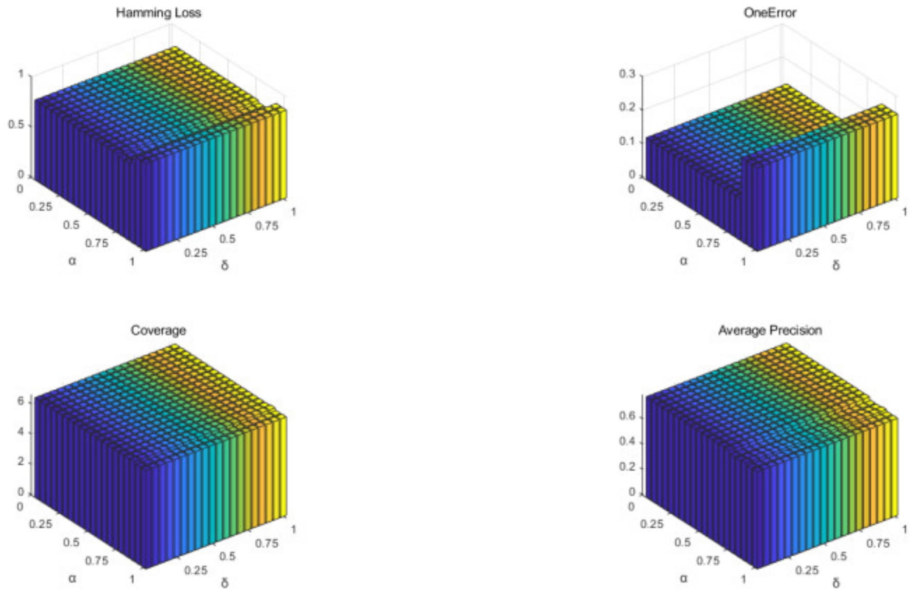
4.2. Effectiveness of Parameters α and δ

In this subsection, we conduct several experiments to analyze the effectiveness of $\alpha$ and $\delta$.

4.2.1. Experimental Settings

For analyzing the effectiveness of parameters, we conduct several experiments. We gradually increase the value of parameter $\alpha$ from 0 to 1 with a step of 0.05 and $\delta$ from 0 to ${10}^{20}$ with a step of ${10}^1$. The experimental result is shown in Figure 1.

4.2.2. Discussions of the Experimental Results

In Figure 1 we can easily observe that with the increase in $\alpha$, the performance of our proposed algorithm decreases when $\alpha$ is close to 1. Parameter $\delta$ does not have a significant effect on performance. It provides the recommended parameter setting for our experiments.

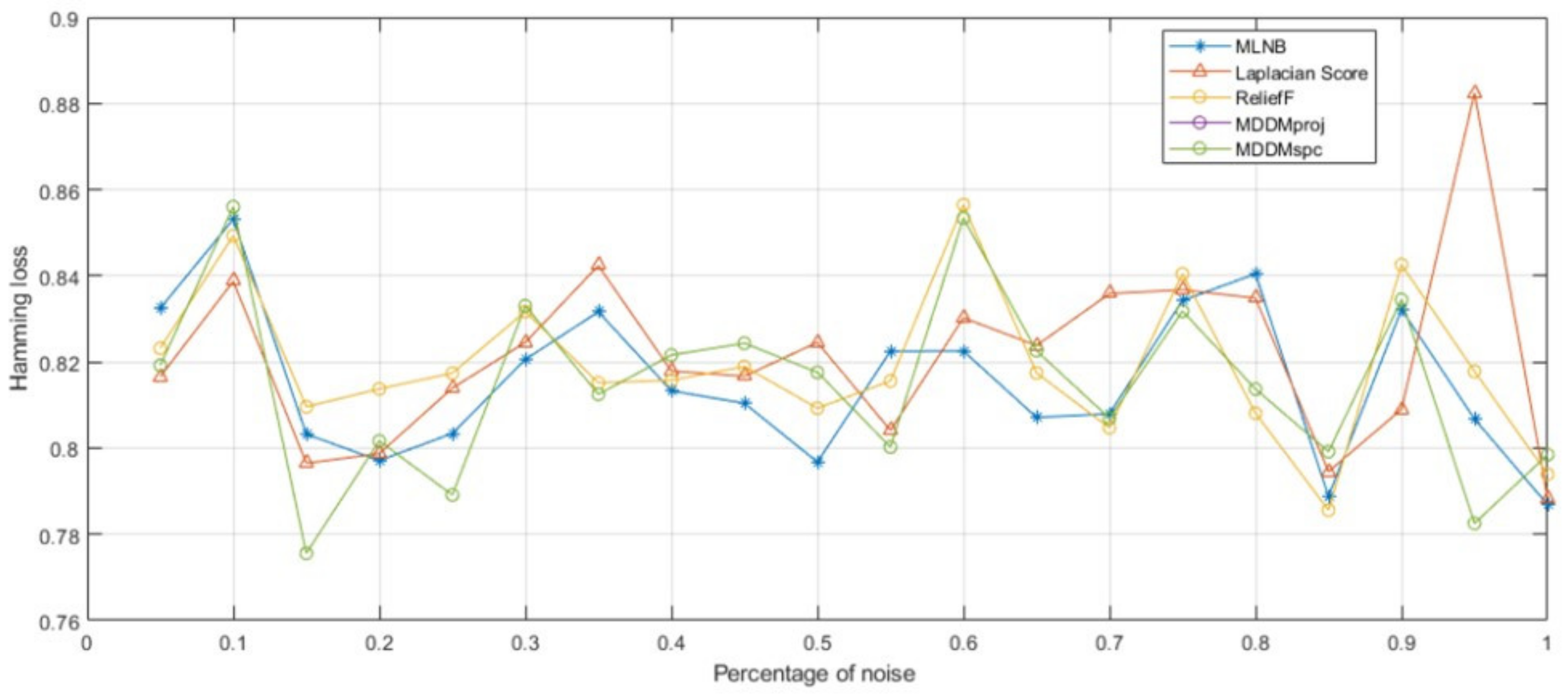
4.3. Effectiveness of Noise

In this subsection, we conduct several experiments to analyze the effectiveness of noise.

4.3.1. Experimental Settings

To analyze the effectiveness of noise, we conduct several experiments. We gradually increase the percentage of noise in the dataset Flags from 0 to 1 with a step of 0.05. The experimental result is shown in Figure 2.

4.3.2. Discussions of the Experimental Results

In Figure 1 we can easily observe that all the algorithms display similar performance with the increasing noise percentage. Compared with another algorithm, our proposed algorithm is not worse than them. In other words, for robustness, the performance of our algorithm is equivalent to comparison algorithms.

5. Conclusions

Attribute reduction in multi-label learning has been a hot topic in recent years. We propose a novel rough set model for multi-label learning and investigate the properties of the proposed model. With the proposed model, a novel feature selection method for multi-label learning is proposed, a novel attribute reduction approach is provided, and its validation is proved by experiments.

In the big data era, calculating the reduction of an attribute set presents great challenges for its high time complexity and dynamic attribute reduction. Algorithms can solve the problem by using previously calculated results. In future work, we will carry on promoting the proposed approach into a dynamic multi-label attribute reduction approach.

References

1. Pawlak, Z. Rough set. Int. J. Comput. Inf. Sci. 1982, 11, 341–356. [Google Scholar] [CrossRef]
2. Ziarko, W. Probabilistic approach to rough sets. Int. J. Approx. Reason. 2008, 49, 272–284. [Google Scholar] [CrossRef]
3. Bazan, J.G.; Nguyen, H.S.; Nguyen, S.H.; Synak, P.; Wróblewski, J. Rough set algorithms in classification problem. In Rough Set Methods and Applications Physical; Springer: Heidelberg, Germany, 2000. [Google Scholar]
4. Lingras, P. Unsupervised Rough Set Classification Using Gas. J. Intell. Inf. Syst. 2001, 16, 215–228. [Google Scholar] [CrossRef]
5. Miao, D.; Duan, Q.; Zhang, H.; Jiao, N. Rough set based hybrid algorithm for text classification. Expert Syst. Appl. 2009, 36, 9168–9174. [Google Scholar] [CrossRef]
6. Sharma, H.K.; Majumder, S.; Biswas, A.; Prentkovskis, O.; Kar, S.; Skačkauskas, P. A Study on Decision-Making of the Indian Railways Reservation System during COVID-19. J. Adv. Transp. 2022, 2022, 7685375. Available online: https://www.hindawi.com/journals/jat/2022/7685375/ (accessed on 7 July 2022). [CrossRef]
7. Lingras, P. Rough set clustering for web mining. In Proceedings of the 2002 IEEE World Congress on Computational Intelligence, 2002 IEEE International Conference on Fuzzy Systems, FUZZ-IEEE’02. Proceedings (Cat. No. 02CH37291), Honolulu, HI, USA, 12–17 May 2002. [Google Scholar]
8. Lingras, P.; Peters, G. Applying rough set concepts to clustering. In Rough Sets: Selected Methods and Applications in Management and Engineering; Springer: London, UK, 2012; pp. 23–37. [Google Scholar]
9. Parmar, D.; Wu, T.; Blackhurst, J. MMR: An algorithm for clustering categorical data using Rough Set Theory. Data Knowl. Eng. 2007, 63, 879–893. [Google Scholar] [CrossRef]
10. Vidhya, K.A.; Geetha, T.V. Rough set theory for document clustering: A review. J. Intell. Fuzzy Syst. 2017, 32, 2165–2185. [Google Scholar] [CrossRef]
11. Hedar, A.R.; Ibrahim, A.M.M.; Abdel-Hakim, A.E.; Sewisy, A.A. Modulated clustering using integrated rough sets and scatter search attribute reduction. In Proceedings of the Genetic and Evolutionary Computation Conference Companion, Kyoto, Japan, 15–19 July 2018; pp. 1394–1401. [Google Scholar]
12. Xia, S.; Zhang, H.; Li, W.; Wang, G.; Giem, E.; Chen, Z. GBNRS: A Novel Rough Set Algorithm for Fast Adaptive Attribute Reduction in Classification. IEEE Trans. Knowl. Data Eng. 2022, 34, 1231–1242. [Google Scholar] [CrossRef]
13. Qian, Y.; Liang, J.; Yao, Y.; Dang, C. MGRS: A multi-granulation rough set. Inf. Sci. 2010, 180, 949–970. [Google Scholar] [CrossRef]
14. Yao, Y.; Yao, B. Covering based rough set approximations. Inf. Sci. 2012, 200, 91–107. [Google Scholar] [CrossRef]
15. Kumar, S.U.; Inbarani, H.H. A Novel Neighborhood Rough Set Based Classification Approach for Medical Diagnosis. Procedia Comput. Sci. 2015, 47, 351–359. [Google Scholar] [CrossRef]
16. Zhang, J.; Li, T.; Ruan, D.; Liu, D. Neighborhood rough sets for dynamic data mining. Int. J. Intell. Syst. 2012, 27, 317–342. [Google Scholar] [CrossRef]
17. Hu, Q.; Yu, D.; Liu, J.; Wu, C. Neighborhood rough set based heterogeneous feature subset selection. Inf. Sci. 2008, 178, 3577–3594. [Google Scholar] [CrossRef]
18. Yong, L.; Wenliang, H.; Yunliang, J.; Zeng, Z. Quick attribute reduce algorithm for neighborhood rough set model. Inf. Sci. 2014, 271, 65–81. [Google Scholar] [CrossRef]
19. Chen, H.; Li, T.; Cai, Y.; Luo, C.; Fujita, H. Parallel attribute reduction in dominance-based neighborhood rough set. Inf. Sci. 2016, 373, 351–368. [Google Scholar] [CrossRef]
20. Zhou, P.; Hu, X.; Li, P.; Wu, X. Online streaming feature selection using adapted Neighborhood Rough Set. Inf. Sci. 2018, 481, 258–279. [Google Scholar] [CrossRef]
21. Sun, L.; Ji, S.; Ye, J. Multi-Label Dimensionality Reduction; CRC Press: Boca Raton, FL, USA, 2016. [Google Scholar] [CrossRef]
22. Fisher, R.A. The use of multiple measurements in taxonomic problems. Ann. Eugen. 1936, 7, 179–188. [Google Scholar] [CrossRef]
23. Wold, H. Estimation of principal components and related models by iterative least squares. In Multivariate Analysis; Academic Press: Cambridge, MA, USA, 1966; pp. 391–420. [Google Scholar]
24. Zhang, Y.; Zhou, Z.H. Multilabel dimensionality reduction via dependence maximization. ACM Trans. Knowl. Discov. Data 2010, 4, 1–21. [Google Scholar] [CrossRef]
25. Zhang, M.-L.; Peña, J.M.; Robles, V. Feature selection for multi-label naïve Bayes classification. Inf. Sci. 2009, 179, 3218–3229. [Google Scholar] [CrossRef]
26. Lin, Y.; Hu, Q.; Liu, J.; Chen, J.; Duan, J. Multi-label feature selection based on neighborhood mutual information. Appl. Soft Comput. 2016, 38, 244–256. [Google Scholar] [CrossRef]
27. Liu, J.; Lin, Y.; Li, Y.; Weng, W.; Wu, S. Online multi-label streaming feature selection based on neighborhood rough set. Pattern Recognit. 2018, 84, 273–287. [Google Scholar] [CrossRef]
28. Deng, Z.; Zheng, Z.; Deng, D.; Wang, T.; He, Y.; Zhang, D. Feature Selection for Multi-Label Learning Based on F-Neighborhood Rough Sets. IEEE Access 2020, 8, 39678–39688. [Google Scholar] [CrossRef]
29. Al-Shami, T.M.; Ciucci, D. Subset neighborhood rough sets. Knowl. Based Syst. 2021, 237, 107868. [Google Scholar] [CrossRef]
30. Chen, Y.; Xue, Y.; Ma, Y.; Xu, F. Measures of uncertainty for neighborhood rough sets. Knowl. Based Syst. 2017, 120, 226–235. [Google Scholar] [CrossRef]
31. Wang, C.; Shi, Y.; Fan, X.; Shao, M. Attribute reduction based on k-nearest neighborhood rough sets. Int. J. Approx. Reason. 2018, 106, 18–31. [Google Scholar] [CrossRef]
32. Li, Y.; Lin, Y.; Liu, J.; Weng, W.; Shi, Z.; Wu, S. Feature selection for multi-label learning based on kernelized fuzzy rough sets. Neurocomputing 2018, 318, 271–286. [Google Scholar] [CrossRef]
33. Xu, J.; Shen, K.; Sun, L. Multi-label feature selection based on fuzzy neighborhood rough sets. Complex Intell. Syst. 2022, 8, 2105–2129. [Google Scholar] [CrossRef]
34. Wang, Q.; Qian, Y.; Liang, X.; Guo, Q.; Liang, J. Local neighborhood rough set. Knowl. Based Syst. 2018, 153, 53–64. [Google Scholar] [CrossRef]
35. Lin, G.; Qian, Y.; Li, J. NMGRS: Neighborhood-based multi-granulation rough sets. Int. J. Approx. Reason. 2012, 53, 1080–1093. [Google Scholar] [CrossRef]
36. Ziarko, W. Variable precision rough set model. J. Comput. Syst. Sci. 1993, 46, 39–59. [Google Scholar] [CrossRef]
37. He, X.; Cai, D.; Niyogi, P. Laplacian score for feature selection. Adv. Neural Inf. Process. Syst. 2005, 18, 1–8. Available online: https://proceedings.neurips.cc/paper/2005/file/b5b03f06271f8917685d14cea7c6c50a-Paper.pdf (accessed on 7 July 2022).
38. Spolaôr, N.; Cherman, E.A.; Monard, M.C.; Lee, H.D. Relief for multi-label feature selection. In Proceedings of the 2013 Brazilian Conference on Intelligent Systems, Fortaleza, Brazil, 20–24 October 2013; IEEE: Manhattan, NY, USA, 2013; pp. 6–11. [Google Scholar]
39. Liu, G.L. Axiomatic systems for rough sets and fuzzy rough sets. Int. J. Approx. Reason. 2008, 48, 857–867. [Google Scholar] [CrossRef]
Figure 1. Effectiveness of parameter α and δ on dataset Emotions.
Symmetry 14 01652 g001
Figure 2. Robustness while adding noise into the dataset Flags.
Symmetry 14 01652 g002