Heisenberg Parabolic Subgroup of SO^∗(10) and Invariant Differential Operators

Abstract

In the present paper we continue the project of systematic construction of invariant differential operators on the example of the non-compact algebra $s{o}^{\ast }\left(10\right)$. We use the maximal Heisenberg parabolic subalgebra $\mathcal{P}=\mathcal{M}\oplus \mathcal{A}\oplus \mathcal{N}$ with $\mathcal{M}=su(3,1)\oplus su\left(2\right)\cong s{o}^{\ast }\left(6\right)\oplus so\left(3\right)$. We give the main and the reduced multiplets of indecomposable elementary representations. This includes the explicit parametrization of the intertwining differential operators between the ERS. Due to the recently established parabolic relations the multiplet classification results are valid also for the algebras $so(p,q)$ (with $p+q=10$, $p\ge q\ge 2$) with maximal Heisenberg parabolic subalgebra: ${\mathcal{P}}^{\prime }={\mathcal{M}}^{\prime }\oplus {\mathcal{A}}^{\prime }\oplus {\mathcal{N}}^{\prime }$, ${\mathcal{M}}^{\prime }=so(p-2,q-2)\oplus sl(2,IR)$, ${\mathcal{M}}^{\prime \mathbb{C}}\cong {\mathcal{M}}^{\mathbb{C}}$.

1. Introduction

Invariant differential operators play a very important role in the description of physical symmetries. Recently, Refs. [1,2] we started the systematic explicit construction of invariant differential operators. We gave an explicit description of the building blocks, namely, the parabolic subgroups and subalgebras from which the necessary representations are induced. Thus, we have set the stage for a study of different non-compact groups.

In the present paper, we focus on the algebra $s{o}^{\ast }\left(10\right)$. The algebras $s{o}^{\ast }\left(2n\right)$ (for $n\ge 2$) form a class of Lie algebras that have maximal Heisenberg parabolic subalgebras. The latter are given as: $\mathcal{P}=\mathcal{M}\oplus \mathcal{A}\oplus \mathcal{N}$, where $\mathcal{M}=s{o}^{\ast }(2n-4)\oplus so\left(3\right)$.

We note that there are low rank level coincidences: $s{o}^{\ast }\left(4\right)\cong so\left(3\right)\oplus so(2,1)$, $s{o}^{\ast }\left(6\right)\cong su(3,1)$, $s{o}^{\ast }\left(8\right)\cong so(6,2)$, which are well studied, cf. e.g., [2].

In order to avoid repetition, we refer to [1,2,3] for motivations and an extensive list of literature on the subject.

2. Preliminaries

Let G be a semisimple non-compact Lie group, and K a maximal compact subgroup of G. Then we have an Iwasawa decomposition $G=K{A}_0{N}_0$, where $A_0$ is abelian simply connected vector subgroup of G, $N_0$ is a nilpotent simply connected subgroup of G preserved by the action of $A_0$. Further, let $M_0$ be the centralizer of $A_0$ in K. Then the subgroup $P_0=M_0{A}_0{N}_0$ is a minimal parabolic subgroup of G. A parabolic subgroup $P=MAN$ is any subgroup of G which contains a minimal parabolic subgroup.

The importance of the parabolic subgroups comes from the fact that the representations induced from them generate all (admissible) irreducible representations of G [4,5,6,7].

Let $\nu$ be a (non-unitary) character of A, $\nu \in {\mathcal{A}}^{\ast }$, let $\mu$ fix an irreducible representation $D^{\mu }$ of M on a vector space $V_{\mu }$.

We call the induced representation $\chi =$ Ind${}_P^G(\mu \otimes \nu \otimes 1)$ an elementary representation of G [8,9]. Their spaces of functions are:

$${\mathcal{C}}_{\chi }=\{\mathcal{F}\in C^{\infty }(G,V_{\mu })|\mathcal{F}\left(gman\right)=e^{-\nu \left(H\right)}·D^{\mu }\left(m^{-1}\right)\mathcal{F}\left(g\right)\}$$

(1)

where $a=exp\left(H\right)\in A$, $H\in \mathcal{A}$, $m\in M$, $n\in N$. The representation action is the $left$ regular action:

$$\left({\mathcal{T}}^{\chi }\left(g\right)\mathcal{F}\right)\left(g^{\prime }\right)=\mathcal{F}\left(g^{-1}{g}^{\prime }\right),g,g^{\prime }\in G.$$

(2)

For our purposes, here we restrict to maximal parabolic subgroups P, so that $\mathrm{rank}A=1$. Thus, for our representations, the character $\nu$ is parameterized by a real number d, called the conformal weight or energy.

An important ingredient in our considerations are the highest/lowest weight representations of ${\mathcal{G}}^{\mathbb{C}}$. These can be realized as (factor-modules of) Verma modules $V^{\mathsf{\Lambda }}$ over ${\mathcal{G}}^{\mathbb{C}}$, where $\mathsf{\Lambda }\in {\left({\mathcal{H}}^{\mathbb{C}}\right)}^{\ast }$, ${\mathcal{H}}^{\mathbb{C}}$ is a Cartan subalgebra of ${\mathcal{G}}^{\mathbb{C}}$, weight $\mathsf{\Lambda }=\mathsf{\Lambda }\left(\chi \right)$ is determined uniquely from $\chi$ [10,11].

Actually, since our ERs will be induced from finite-dimensional representations of $\mathcal{M}$ (or their limits) the Verma modules are always reducible. Thus, it is more convenient to use generalized Verma modules ${\tilde{V}}^{\mathsf{\Lambda }}$ such that the role of the highest/lowest weight vector $v_0$ is taken by the space $V_{\mu }{v}_0$. For the generalized Verma modules (GVMs) the reducibility is controlled only by the value of the conformal weight d. Relatedly, for the intertwining differential operators only the reducibility w.r.t. non-compact roots is essential.

Another main ingredient of our approach is as follows. We group the (reducible) ERs with the same Casimirs in sets called multiplets [11,12]. The multiplet corresponding to fixed values of the Casimirs may be depicted as a connected graph, the vertices of which correspond to the reducible ERs and the lines between the vertices correspond to intertwining operators. The explicit parametrization of the multiplets and their ERs is important for the understanding of the situation.

In fact, the multiplets contain explicitly all the data necessary to construct the intertwining differential operators. Actually, the data for each intertwining differential operator consists of the pair $(\beta ,m)$, where $\beta$ is a (non-compact) positive root of ${\mathcal{G}}^{\mathbb{C}}$, $m\in IN$, such that the BGG [13] Verma module reducibility condition (for highest weight modules) is fulfilled:

$$(\mathsf{\Lambda }+\rho ,{\beta }^{\vee })=m,{\beta }^{\vee }\equiv 2\beta /(\beta ,\beta ).$$

(3)

When (3) holds then the Verma module with shifted weight $V^{\mathsf{\Lambda }-m\beta }$ (or ${\tilde{V}}^{\mathsf{\Lambda }-m\beta }$ for GVM and $\beta$ non-compact) is embedded in the Verma module $V^{\mathsf{\Lambda }}$ (or ${\tilde{V}}^{\mathsf{\Lambda }}$). This embedding is realized by a singular vector $v_s$ determined by a polynomial ${\mathcal{P}}_{m,\beta }\left({\mathcal{G}}^{-}\right)$ in the universal enveloping algebra $\left(U\left({\mathcal{G}}_{-}\right)\right)v_0$, ${\mathcal{G}}^{-}$ is the subalgebra of ${\mathcal{G}}^{\mathbb{C}}$ generated by the negative root generators [14]. More explicitly, ref. [11], $v_{m,\beta }^s={\mathcal{P}}_{\beta }^m{v}_0$ (or $v_{m,\beta }^s={\mathcal{P}}_{\beta }^m{V}_{\mu }{v}_0$ for GVMs). Then there exists [11] an intertwining differential operator

$${\mathcal{D}}_{\beta }^m:{\mathcal{C}}_{\chi \left(\mathsf{\Lambda }\right)}⟶{\mathcal{C}}_{\chi (\mathsf{\Lambda }-m\beta )}$$

(4)

given explicitly by:

$${\mathcal{D}}_{\beta }^m={\mathcal{P}}_{\beta }^m\left(\widehat{{\mathcal{G}}^{-}}\right)$$

(5)

where $\widehat{{\mathcal{G}}^{-}}$ denotes the $right$ action on the functions $\mathcal{F}$, cf. (1).

3. The Non-Compact Lie Algebra so^∗(10)

3.1. The General Case of so^∗(2n)

The group $G=S{O}^{\ast }\left(2n\right)$ consists of all matrices in $SO(2n,\mathbb{C})$ which commute with a real skew-symmetric matrix times the complex conjugation operator C:

$$S{O}^{\ast }\left(2n\right)\doteq \{g\in SO(2n,\mathbb{C})|J_{n}Cg=g{J}_{n}C\}$$

(6)

The Lie algebra $\mathcal{G}=s{o}^{\ast }\left(2n\right)$ is given by:

$$\begin{array}{ccc}\hfill s{o}^{\ast }\left(2n\right)& \doteq & \{X\in so(2n,\mathbb{C})|J_{n}CX=X{J}_{n}C\}=\hfill \\ & =& \{X=\left(\begin{array}{cc}a& b\\ -\overline{b}& \overline{a}\end{array}\right)|a,b\in gl(n,\mathbb{C}),{}^{t}a=-a,b^{†}=b\}.\hfill \end{array}$$

(7)

${dim}_R\mathcal{G}=n(2n-1)$, $\mathrm{rank}\mathcal{G}=n$.

The Cartan involution is given by: $\mathsf{\Theta }X=-X^{†}$. Thus, $\mathcal{K}\cong u\left(n\right)$:

$$\mathcal{K}=\{X=\left(\begin{array}{cc}a& b\\ -b& a\end{array}\right)|a,b\in gl(n,\mathbb{C}),{}^{t}a=-a=-\overline{a},b^{†}=b=\overline{b}\}.$$

(8)

Thus, $\mathcal{G}=s{o}^{\ast }\left(2n\right)$ has discrete series representations and highest/lowest weight representations. The complementary space $\mathcal{P}$ is given by:

$$\mathcal{P}=\{X=\left(\begin{array}{cc}a& b\\ b& -a\end{array}\right)|a,b\in gl(n,\mathbb{C}),{}^{t}a=-a=\overline{a},b^{†}=b=-\overline{b}\}.$$

(9)

${dim}_R\mathcal{P}=n(n-1)$. The split rank is $r\equiv [n/2]$.

We need also the root system of ${\mathcal{G}}^{\mathbb{C}}=so(2n,\mathbb{C})$. The positive roots are given standardly as:

$$\begin{array}{ccc}\hfill {\alpha }_{ij}& =& {ϵ}_i-{ϵ}_j,1\le i<j\le n,\hfill \end{array}$$

(10a)

$$\begin{array}{ccc}\hfill {\beta }_{ij}& =& {ϵ}_i+{ϵ}_j,1\le i<j\le n\hfill \end{array}$$

(10b)

where ${ϵ}_i$ are standard orthonormal basis: $\langle {ϵ}_i,{ϵ}_j\rangle ={\delta }_{ij}$. We shall need the scalar products of the roots:

$$\begin{array}{c}\hfill \langle {\alpha }_{ij},{\alpha }_{k\ell }\rangle ={\delta }_{ik}-{\delta }_{i\ell }-{\delta }_{jk}+{\delta }_{j\ell }\end{array}$$

(11a)

$$\begin{array}{c}\hfill \langle {\alpha }_{ij},{\beta }_{k\ell }\rangle ={\delta }_{ik}+{\delta }_{i\ell }-{\delta }_{jk}-{\delta }_{j\ell }\end{array}$$

(11b)

$$\begin{array}{c}\hfill \langle {\beta }_{ij},{\beta }_{k\ell }\rangle ={\delta }_{ik}+{\delta }_{i\ell }+{\delta }_{jk}+{\delta }_{j\ell }\end{array}$$

(11c)

Note that the highest root is ${\beta }_{12}$.

The simple roots are:

$$\pi =\{{\gamma }_i={\alpha }_{i,i+1},1\le i\le n-1,{\gamma }_n={\beta }_{n-1,n}\}$$

(12)

The compact roots w.r.t. the real form $S{O}^{\ast }\left(2n\right)$ are ${\alpha }_{ij}$ - they form (by restriction) the root system of the semisimple part of ${\mathcal{K}}^{\mathbb{C}}$, namely, ${\mathcal{K}}_s^{\mathbb{C}}\cong su{\left(n\right)}^{\mathbb{C}}\cong sl(n,\mathbb{C})$, while the roots ${\beta }_{ij}$ are noncompact.

The minimal parabolics of $S{O}^{\ast }\left(2n\right)$ depend on whether n is even or odd and are:

$$\begin{array}{}\hfill \mathrm{(13a)}& \hfill {\mathcal{M}}_0& =& so\left(3\right)\oplus \cdots \oplus so\left(3\right),r\mathrm{factors},\mathrm{for}n=2r\hfill \hfill \mathrm{(13b)}& & =& so\left(2\right)\oplus so\left(3\right)\oplus \cdots \oplus so\left(3\right),r\mathrm{factors},\mathrm{for}n=2r+1\hfill \end{array}$$

The subalgebras ${\mathcal{N}}_0^{\pm }$ which form the root spaces of the root system $(\mathcal{G},{\mathcal{A}}_0)$ are of real dimension $n(n-1)-[n/2]$.

The maximal parabolic subalgebras have $\mathcal{M}$-factors as follows [1]:

$${\mathcal{M}}_j^{\max }=s{o}^{\ast }(2n-4j)\oplus s{u}^{\ast }\left(2j\right),j=1,\dots ,r.$$

(14)

The ${\mathcal{N}}^{\pm }$ factors in the maximal parabolic subalgebras have dimensions: $dim{\left({\mathcal{N}}_j^{\pm }\right)}^{\max }=$$j(4n-6j-1)$.

The case $j=1$ is special. In this case, we have a maximal Heisenberg parabolic with $\mathcal{M}$-factor:

$${\mathcal{M}}_{\mathrm{Heisenberg}}^{\max }=s{o}^{\ast }(2n-4)\oplus su\left(2\right)$$

(15)

which we use in this paper.

3.2. The Case so^∗(10)

Further, we restrict to our case of study $\mathcal{G}=s{o}^{\ast }\left(10\right)$ with minimal parabolic:

$${\mathcal{M}}_0=so\left(2\right)\oplus so\left(3\right)\oplus so\left(3\right)$$

(16)

The Satake-Dynkin diagram of $\mathcal{G}$ is:

(17)

where, by standard convention, the black dots represent the $so\left(3\right)$ subalgebras of ${\mathcal{M}}_0$, and the left-right arrow represents the $so\left(2\right)$ subalgebra of ${\mathcal{M}}_0$.

We shall use the Heisenberg maximal parabolic (15) with $\mathcal{M}$-subalgebra:

$$\mathcal{M}=s{o}^{\ast }\left(6\right)\oplus so\left(3\right)\cong su(3,1)\oplus su\left(2\right)$$

(18)

The Satake-Dynkin diagram of $\mathcal{M}$ is a subdiagram of (17):

(19)

where the single black dot represents the $so\left(3\right)$ subalgebra, while the connected part of the diagram represents the $su(3,1)$ subalgebra.

From the above follows that the $\mathcal{M}$-compact roots of ${\mathcal{G}}^{\mathbb{C}}$ are (given in terms of the simple roots):

$$\begin{array}{}\hfill \mathrm{(20a)}& {\alpha }_{12}={\gamma }_1,\hfill \hfill \mathrm{(20b)}& {\alpha }_{34}={\gamma }_3,{\alpha }_{45}={\gamma }_4,{\beta }_{45}={\gamma }_5,\hfill \hfill & {\alpha }_{35}={\gamma }_3+{\gamma }_4,{\beta }_{34}={\gamma }_3+{\gamma }_4+{\gamma }_5,{\beta }_{35}={\gamma }_3+{\gamma }_5\hfill \end{array}$$

By definition the above are the positive roots of ${\mathcal{M}}^{\mathbb{C}}$, namely: $su{\left(2\right)}^{\mathbb{C}}$ (20a), and $su{(3,1)}^{\mathbb{C}}=sl(4,\mathbb{C})$ (20b).

The positive $\mathcal{M}$-noncompact roots of ${\mathcal{G}}^{\mathbb{C}}$ in terms of the simple roots are:

$$\begin{array}{}\hfill & {\gamma }_{12}={\gamma }_1+{\gamma }_2,{\gamma }_{13}={\gamma }_1+{\gamma }_2+{\gamma }_3,{\gamma }_{14}={\gamma }_1+{\gamma }_2+{\gamma }_3+{\gamma }_4,\hfill \hfill \left(21\mathrm{a}\right)& {\gamma }_2,{\gamma }_{23}={\gamma }_2+{\gamma }_3,{\gamma }_{24}={\gamma }_2+{\gamma }_3+{\gamma }_4,\hfill \hfill & {\beta }_{12}={\gamma }_1+2{\gamma }_2+2{\gamma }_3+{\gamma }_4+{\gamma }_5,{\beta }_{13}={\gamma }_1+{\gamma }_2+2{\gamma }_3+{\gamma }_4+{\gamma }_5,\hfill \hfill & {\beta }_{14}={\gamma }_1+{\gamma }_2+{\gamma }_3+{\gamma }_4+{\gamma }_5,{\beta }_{15}={\gamma }_1+{\gamma }_2+{\gamma }_3+{\gamma }_5,\hfill \hfill & {\beta }_{23}={\gamma }_2+2{\gamma }_3+{\gamma }_4+{\gamma }_5,{\beta }_{24}={\gamma }_2+{\gamma }_3+{\gamma }_4+{\gamma }_5,\hfill \hfill \mathrm{(21b)}& {\beta }_{25}={\gamma }_2+{\gamma }_3+{\gamma }_5\hfill \end{array}$$

where for convenience we use the notation ${\gamma }_{ij}\equiv {\alpha }_{i,j+1}$

To characterize the Verma modules we shall use first the Dynkin labels:

$$m_i\equiv (\mathsf{\Lambda }+\rho ,{\gamma }_i^{\vee })=(\mathsf{\Lambda }+\rho ,{\gamma }_i),i=1,\dots ,5,$$

(22)

where $\rho$ is half the sum of the positive roots of ${\mathcal{G}}^{\mathbb{C}}$. Thus, we shall use:

$${\chi }_{\mathsf{\Lambda }}=\{m_1,m_2,m_3,m_4,m_5\}$$

(23)

Note that when all $m_i\in IN$ then ${\chi }_{\mathsf{\Lambda }}$ characterizes the finite-dimensional irreps of ${\mathcal{G}}^{\mathbb{C}}$ and its real forms, in particular, $s{o}^{\ast }\left(10\right)$. Furthermore, $m_1\in IN$ characterizes the finite-dimensional irreps of the $su\left(2\right)$ subalgebra, while the set of positive integers $\{m_3,m_4,m_5\}$ characterizes the finite-dimensional irreps of $su(3,1)$.

For the $\mathcal{M}$-noncompact roots of ${\mathcal{G}}^{\mathbb{C}}$ we shall use also the Harish-Chandra parameters:

$$\begin{array}{ccc}\hfill m_{ij}& =& (\mathsf{\Lambda }+\rho ,{\gamma }_{ij}^{\vee }),\hfill \end{array}$$

(24a)

$$\begin{array}{ccc}\hfill {\widehat{m}}_{ij}& =& (\mathsf{\Lambda }+\rho ,{\beta }_{ij}^{\vee })\hfill \end{array}$$

(24b)

and explicitly in terms of the Dynkin labels (compare (21)):

$$\begin{array}{}\hfill & \hfill {\chi }_{HC}& =& \{m_{12}=m_1+m_2,m_{13}=m_1+m_2+m_3,\hfill \hfill & & & m_{14}=m_1+m_2+m_3+m_4,m_2,\hfill \hfill \mathrm{(25a)}& & & m_{23}=m_2+m_3,m_{24}=m_2+m_3+m_4,\hfill \hfill & & & {\widehat{m}}_{12}=m_1+2m_2+2m_3+m_4+m_5,\hfill \hfill & & & {\widehat{m}}_{13}=m_1+m_2+2m_3+m_4+m_5,\hfill \hfill & & & {\widehat{m}}_{14}=m_1+m_2+m_3+m_4+m_5,\hfill \hfill & & & {\widehat{m}}_{15}=m_1+m_2+m_3+m_5,\hfill \hfill & & & {\widehat{m}}_{23}=m_2+2m_3+m_4+m_5,\hfill \hfill & & & {\widehat{m}}_{24}=m_2+m_3+m_4+m_5,\hfill \hfill \mathrm{(25b)}& & & {\widehat{m}}_{25}=m_2+m_3+m_5\}\hfill \end{array}$$

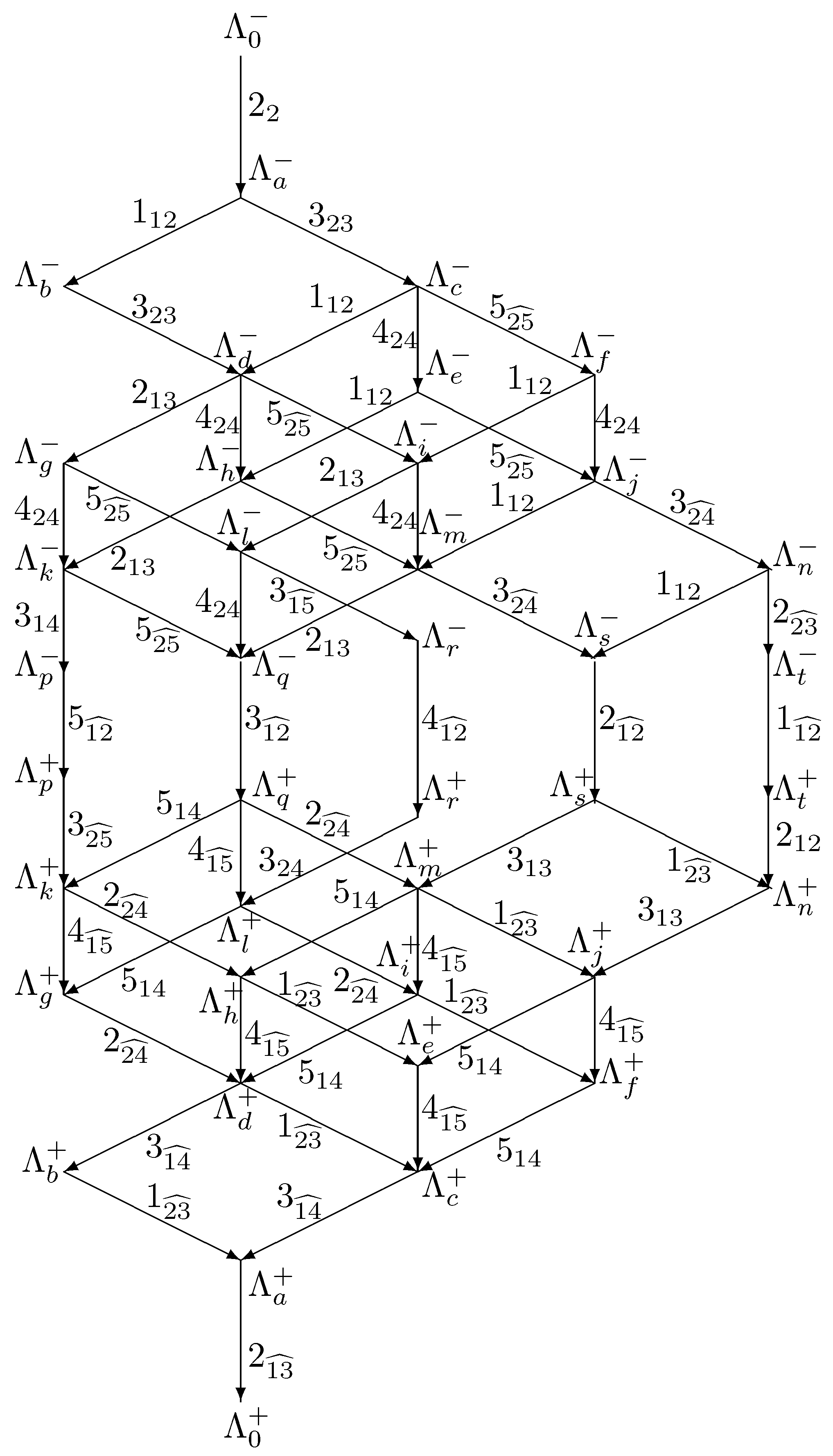
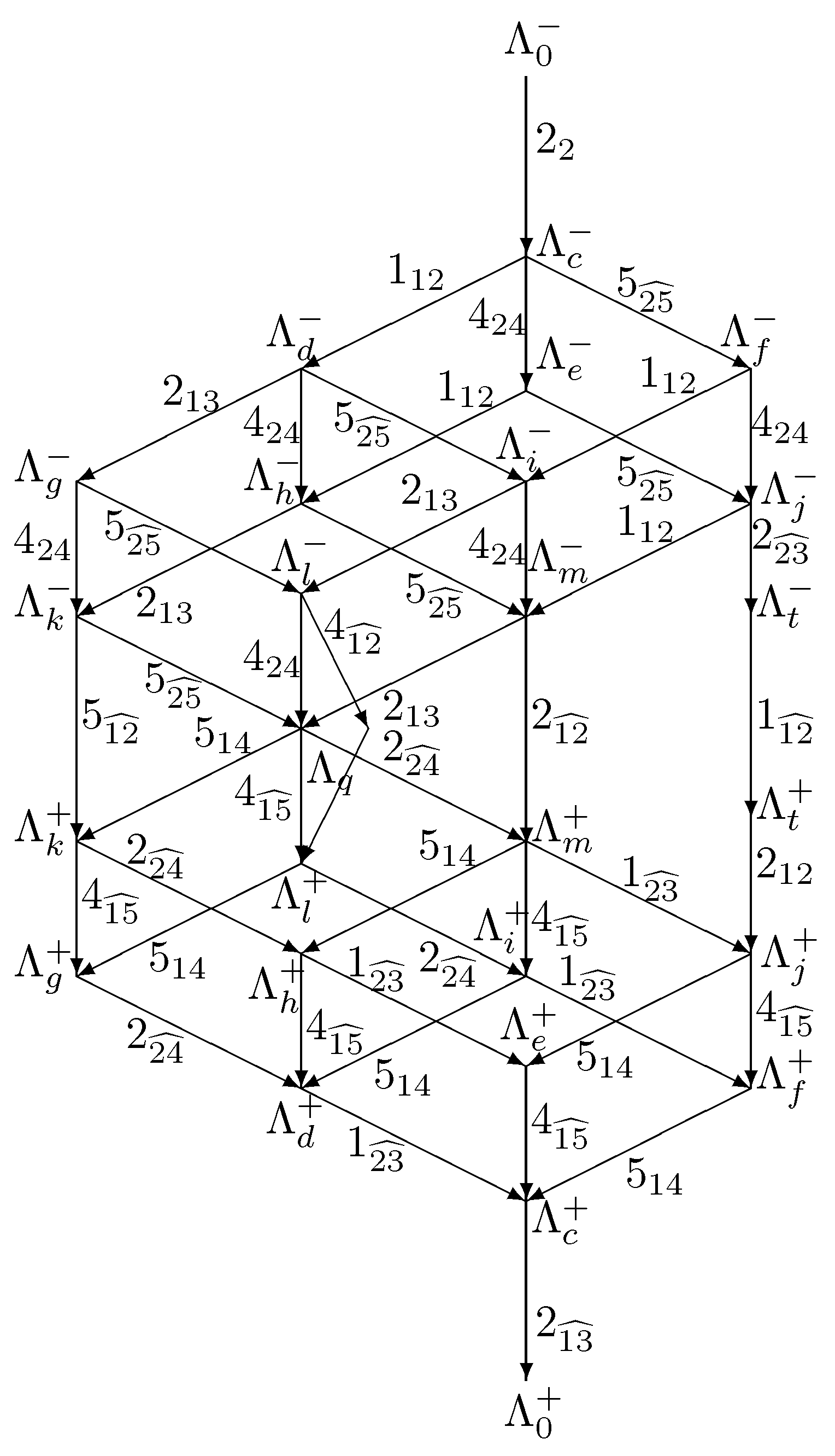
4. Main Multiplets of SO^∗(10)

The main multiplets are in 1-to-1 correspondence with the finite-dimensional irreps of $s{o}^{\ast }\left(10\right)$, i.e., they are labeled by the five positive Dynkin labels $m_i\in IN$.

We take ${\chi }_0={\chi }_{HC}$. It has one embedded Verma module with HW ${\mathsf{\Lambda }}_a={\mathsf{\Lambda }}_0-m_2{\gamma }_2$. The number of ERs/GVMs in the main multiplet is 40. We give the whole multiplet as follows:

$$\begin{array}{ccc}\hfill {\chi }_0& =& \{m_1,m_2,m_3,m_4,m_5\}\hfill \\ \hfill {\chi }_a& =& \{m_{12},-m_2,m_{23},m_4,m_5\},{\mathsf{\Lambda }}_a={\mathsf{\Lambda }}_0-m_2{\gamma }_2\hfill \\ \hfill {\chi }_b& =& \{m_2,-m_{12},m_{13},m_4,m_5\},{\mathsf{\Lambda }}_b={\mathsf{\Lambda }}_a-m_1{\gamma }_{12}\hfill \\ \hfill {\chi }_c& =& \{m_{13},-m_{23},m_2,m_{34},m_{3,5}\},{\mathsf{\Lambda }}_c={\mathsf{\Lambda }}_a-m_3{\gamma }_{23}\hfill \\ \hfill {\chi }_d& =& \{m_{23},-m_{13},m_{12},m_{34},m_{3,5}\},{\mathsf{\Lambda }}_d={\mathsf{\Lambda }}_b-m_3{\gamma }_{23}={\mathsf{\Lambda }}_c-m_1{\gamma }_{12}\hfill \\ \hfill {\chi }_e& =& \{m_{14},-m_{24},m_2,m_3,m_{35}\},{\mathsf{\Lambda }}_e={\mathsf{\Lambda }}_c-m_4{\gamma }_{24}\hfill \\ \hfill {\chi }_f& =& \{m_{13,5},-m_{23,5},m_2,m_{35},m_3\},{\mathsf{\Lambda }}_f={\mathsf{\Lambda }}_c-m_5{\beta }_{25}\hfill \\ \hfill {\chi }_g& =& \{m_3,-m_{13},m_1,m_{24},m_{23,5}\},{\mathsf{\Lambda }}_g={\mathsf{\Lambda }}_d-m_2{\gamma }_{13}\hfill \\ \hfill {\chi }_h& =& \{m_{24},-m_{14},m_{12},m_3,m_{35}\},{\mathsf{\Lambda }}_h={\mathsf{\Lambda }}_d-m_4{\gamma }_{24}\hfill \\ \hfill {\chi }_i& =& \{m_{23,5},-m_{13,5},m_{12},m_{35},m_3\},{\mathsf{\Lambda }}_i={\mathsf{\Lambda }}_d-m_5{\beta }_{25}={\mathsf{\Lambda }}_f-m_1{\gamma }_{13}\hfill \\ \hfill {\chi }_j& =& \{m_{15},-m_{25},m_2,m_{3,5},m_{34}\},{\mathsf{\Lambda }}_j={\mathsf{\Lambda }}_e-m_5{\beta }_{25}\hfill \\ \hfill {\chi }_k& =& \{m_{34},-m_{14},m_1,m_{23},m_{25}\},{\mathsf{\Lambda }}_k={\mathsf{\Lambda }}_g-m_4{\gamma }_{24}={\mathsf{\Lambda }}_h-m_2{\gamma }_{13}\hfill \\ \hfill {\chi }_l& =& \{m_{3,5},-m_{13,5},m_1,m_{25},m_{23}\},{\mathsf{\Lambda }}_l={\mathsf{\Lambda }}_g-m_5{\beta }_{25}\hfill \\ \hfill {\chi }_m& =& \{m_{25},-m_{15},m_{12},m_{3,5},m_{34}\},{\mathsf{\Lambda }}_m={\mathsf{\Lambda }}_h-m_5{\beta }_{25}\hfill \\ \hfill {\chi }_n& =& \{m_{15,3},-m_{25,3},m_{23},m_5,m_4\},{\mathsf{\Lambda }}_n={\mathsf{\Lambda }}_j-m_3{\beta }_{24}\hfill \\ \hfill {\chi }_p& =& \{m_4,-m_{14},m_1,m_2,m_{25,3}\},{\mathsf{\Lambda }}_p={\mathsf{\Lambda }}_k-m_3{\gamma }_{14}\hfill \\ \hfill {\chi }_q& =& \{m_{35},-m_{15},m_1,m_{23,5},m_{24}\},{\mathsf{\Lambda }}_q={\mathsf{\Lambda }}_k-m_5{\beta }_{25}\hfill \\ \hfill {\chi }_r& =& \{m_5,-m_{13,5},m_1,m_{25,3},m_2\},{\mathsf{\Lambda }}_r={\mathsf{\Lambda }}_l-m_3{\beta }_{15}\hfill \\ \hfill {\chi }_s& =& \{m_{25,3},-m_{15,3},m_{13},m_5,m_4\},{\mathsf{\Lambda }}_s={\mathsf{\Lambda }}_m-m_3{\beta }_{24}\hfill \\ \hfill {\chi }_t& =& \{m_{15,23},-m_{25,3},m_3,m_5,m_4\},{\mathsf{\Lambda }}_t={\mathsf{\Lambda }}_n-m_2{\beta }_{23}\hfill \end{array}$$

(26)

$$\begin{array}{ccc}\hfill {\chi }_p^{+}& =& \{m_4,-m_{15},m_1,m_2,m_{25,3}\},{\mathsf{\Lambda }}_p^{+}={\mathsf{\Lambda }}_p-m_5{\beta }_{12}\hfill \\ \hfill {\chi }_q^{+}& =& \{m_{35},-m_{15,3},m_1,m_{23,5},m_{24}\},{\mathsf{\Lambda }}_q^{+}={\mathsf{\Lambda }}_q-m_3{\beta }_{12}\hfill \\ \hfill {\chi }_r^{+}& =& \{m_5,-m_{15},m_1,m_{25,3},m_2\},{\mathsf{\Lambda }}_r^{+}={\mathsf{\Lambda }}_r-m_4{\beta }_{12}\hfill \\ \hfill {\chi }_s^{+}& =& \{m_{25,3},-m_{15,23},m_{13},m_5,m_4\},{\mathsf{\Lambda }}_s^{+}={\mathsf{\Lambda }}_s-m_2{\beta }_{12}\hfill \\ \hfill {\chi }_t^{+}& =& \{m_{15,23},-m_{15,3},m_3,m_5,m_4\},{\mathsf{\Lambda }}_t^{+}={\mathsf{\Lambda }}_t-m_1{\beta }_{12}\hfill \\ \hfill {\chi }_k^{+}& =& \{m_{34},-m_{15,3},m_1,m_{23},m_{25}\},{\mathsf{\Lambda }}_k^{+}={\mathsf{\Lambda }}_p^{+}-m_3{\beta }_{25}\hfill \\ \hfill {\chi }_l^{+}& =& \{m_{3,5},-m_{15,3},m_1,m_{25},m_{23}\},{\mathsf{\Lambda }}_l^{+}={\mathsf{\Lambda }}_q^{+}-m_4{\beta }_{15}={\mathsf{\Lambda }}_r^{+}-m_3{\gamma }_{24}\hfill \\ \hfill {\chi }_m^{+}& =& \{m_{25},-m_{15,23},m_{12},m_{3,5},m_{34}\},{\mathsf{\Lambda }}_m^{+}={\mathsf{\Lambda }}_q^{+}-m_2{\beta }_{24}={\mathsf{\Lambda }}_s^{+}-m_3{\gamma }_{13}\hfill \\ \hfill {\chi }_n^{+}& =& \{m_{15,3},-m_{15,23},m_{23},m_5,m_4\},{\mathsf{\Lambda }}_n^{+}={\mathsf{\Lambda }}_s^{+}-m_1{\beta }_{23}={\mathsf{\Lambda }}_t^{+}-m_2{\gamma }_{12}\hfill \\ \hfill {\chi }_h^{+}& =& \{m_{24},-m_{15,23},m_{12},m_3,m_{35}\},{\mathsf{\Lambda }}_h^{+}={\mathsf{\Lambda }}_k^{+}-m_2{\beta }_{24}={\mathsf{\Lambda }}_m^{+}-m_5{\gamma }_{14}\hfill \\ \hfill {\chi }_g^{+}& =& \{m_3,-m_{15,3},m_1,m_{24},m_{23,5}\},{\mathsf{\Lambda }}_{\omega }^{+}={\mathsf{\Lambda }}_l^{+}-m_5{\gamma }_{14}\hfill \\ \hfill {\chi }_i^{+}& =& \{m_{23,5},-m_{15,23},m_{12},m_{35},m_3\},{\mathsf{\Lambda }}_{\tau }^{+}={\mathsf{\Lambda }}_l^{+}-m_2{\beta }_{24}={\mathsf{\Lambda }}_m^{+}-m_4{\beta }_{15}\hfill \\ \hfill {\chi }_j^{+}& =& \{m_{15},-m_{15,23},m_2,m_{3,5},m_{34}\},{\mathsf{\Lambda }}_{\pi }^{+}={\mathsf{\Lambda }}_m^{+}-m_1{\beta }_{23}={\mathsf{\Lambda }}_n^{+}-m_3{\gamma }_{13}\hfill \\ \hfill {\chi }_e^{+}& =& \{m_{14},-m_{15,23},m_2,m_3,m_{35}\},{\mathsf{\Lambda }}_{\alpha }^{+}={\mathsf{\Lambda }}_h^{+}-m_1{\beta }_{23}\hfill \\ \hfill {\chi }_d^{+}& =& \{m_{23},-m_{15,23},m_{12},m_{34},m_{3,5}\},{\mathsf{\Lambda }}_{\beta }^{+}={\mathsf{\Lambda }}_g^{+}-m_2{\beta }_{24}={\mathsf{\Lambda }}_i^{+}-m_5{\gamma }_{14}\hfill \\ \hfill {\chi }_f^{+}& =& \{m_{13,5},-m_{15,23},m_2,m_{35},m_3\},{\mathsf{\Lambda }}_{\gamma }^{+}={\mathsf{\Lambda }}_i^{+}-m_1{\beta }_{23}={\mathsf{\Lambda }}_j^{+}-m_4{\beta }_{15}\hfill \\ \hfill {\chi }_b^{+}& =& \{m_2,-m_{15,23},m_{13},m_4,m_5\},{\mathsf{\Lambda }}_{ϵ}^{+}={\mathsf{\Lambda }}_{\beta }^{+}-m_3{\beta }_{14}\hfill \\ \hfill {\chi }_c^{+}& =& \{m_{13},-m_{15,23},m_2,m_{34},m_{3,5}\},{\mathsf{\Lambda }}_{\lambda }^{+}={\mathsf{\Lambda }}_d^{+}-m_1{\beta }_{23}\hfill \\ \hfill {\chi }_a^{+}& =& \{m_{12},-m_{15,23},m_{23},m_4,m_5\},{\mathsf{\Lambda }}_{\kappa }^{+}={\mathsf{\Lambda }}_b^{+}-m_1{\beta }_{23}={\mathsf{\Lambda }}_c^{+}-m_3{\beta }_{14}\hfill \\ \hfill {\chi }_0^{+}& =& \{m_1,-m_{15,3},m_3,m_4,m_5\},{\mathsf{\Lambda }}_0^{+}={\mathsf{\Lambda }}_a^{+}-m_2{\beta }_{13}\hfill \end{array}$$

(27)

We shall label the signature of the ERs of $\mathcal{G}$ also as follows:

$$\chi =[n;c;n_1,n_2,n_3],n\in IN,c=-\frac{1}{2}{m}_{15,23},n_j=m_{j+2}\in {\mathbb{Z}}_{+},$$

(28)

where the first entry $n=m_1$ labels the finite-dimensional irreps of $su\left(2\right)$, the second entry labels the characters of $\mathcal{A}$, the last three entries of $\chi$ are labels of the finite-dimensional (nonunitary) irreps of $\mathcal{M}=su(3,1)$ when all $n_j>0$ or limits of the latter when some $n_j=0$. Note that $m_{15,23}=m_1+2m_2+2m_3+m_4+m_5$ is the Harish-Chandra parameter for the highest root ${\beta }_{12}$.

These labeling signatures may be given in the following pair-wise manner:

$$\begin{array}{ccc}\hfill {\chi }_0^{\pm }& =& [m_1;m_3,m_4,m_5;\pm \frac{1}{2}{m}_{15,23}]\hfill \\ \hfill {\chi }_a^{\pm }& =& [m_{12};m_{23},m_4,m_5;\pm \frac{1}{2}{m}_{15,3}]\hfill \\ \hfill {\chi }_b^{\pm }& =& [m_2;m_{13},m_4,m_5;\pm \frac{1}{2}{m}_{25,3}]\hfill \\ \hfill {\chi }_c^{\pm }& =& [m_{13};m_2,m_{34},m_{3,5};\pm \frac{1}{2}{m}_{15}]\hfill \\ \hfill {\chi }_d^{\pm }& =& [m_{23};m_{12},m_{34},m_{3,5};\pm \frac{1}{2}{m}_{25}]\hfill \\ \hfill {\chi }_e^{\pm }& =& [m_{14};m_2,m_3,m_{35};\pm \frac{1}{2}{m}_{13,5}]\hfill \\ \hfill {\chi }_f^{\pm }& =& [m_{13,5};m_2,m_{35},m_3;\pm \frac{1}{2}{m}_{14}]\hfill \\ \hfill {\chi }_g^{\pm }& =& [m_3;m_1,m_{24},m_{23,5};\pm \frac{1}{2}{m}_{35}]\hfill \\ \hfill {\chi }_h^{\pm }& =& [m_{24};m_{12},m_3,m_{35};\pm \frac{1}{2}{m}_{23,5}]\hfill \\ \hfill {\chi }_i^{\pm }& =& [m_{23,5};m_{12},m_{35},m_3;\pm \frac{1}{2}{m}_{24}]\hfill \\ \hfill {\chi }_j^{\pm }& =& [m_{15};m_2,m_{3,5},m_{34};\pm \frac{1}{2}{m}_{13}]\hfill \\ \hfill {\chi }_k^{\pm }& =& [m_{34};m_1,m_{23},m_{25};\pm \frac{1}{2}{m}_{3,5}]\hfill \\ \hfill {\chi }_l^{\pm }& =& [m_{3,5};m_1,m_{25},m_{23};\pm \frac{1}{2}{m}_{34}]\hfill \\ \hfill {\chi }_m^{\pm }& =& [m_{25};m_{12},m_{3,5},m_{34};\pm \frac{1}{2}{m}_{23}]\hfill \\ \hfill {\chi }_n^{\pm }& =& [m_{15,3};m_{23},m_5,m_4;\pm \frac{1}{2}{m}_{12}]\hfill \\ \hfill {\chi }_p^{\pm }& =& [m_4;m_1,m_2,m_{25,3};\pm \frac{1}{2}{m}_5]\hfill \\ \hfill {\chi }_q^{\pm }& =& [m_{35};m_1,m_{23,5},m_{24};\pm \frac{1}{2}{m}_3]\hfill \\ \hfill {\chi }_r^{\pm }& =& [m_5;m_1,m_{25,3},m_2;\pm \frac{1}{2}{m}_4]\hfill \\ \hfill {\chi }_s^{\pm }& =& [m_{25,3};m_{13},m_5,m_4;\pm \frac{1}{2}{m}_2]\hfill \\ \hfill {\chi }_t^{\pm }& =& [m_{15,23};m_3,m_5,m_4;\pm \frac{1}{2}{m}_1]\hfill \end{array}$$

The ERs in the multiplet are related also by intertwining integral operators introduced in [15,16]. These operators are defined for any ER, the general action being:

$$\begin{array}{ccc}\hfill & & G_{KS}:{\mathcal{C}}_{\chi }⟶{\mathcal{C}}_{{\chi }^{\prime }},\hfill \\ & & \chi =\{n;n_1,n_2,n_3;c\},{\chi }^{\prime }=\{n;n_1,n_2,n_3;-c\}.\hfill \end{array}$$

(29)

The main multiplets are given explicitly in Figure 1. The pairs ${\chi }^{\pm }$ are symmetric w.r.t. to the dashed line in the middle of the figure—this represents the Weyl symmetry realized by the Knapp-Stein operators (29): $G_{KS}:{\mathcal{C}}_{{\chi }^{\mp }}⟷{\mathcal{C}}_{{\chi }^{\pm }}$.

Some comments are in order.

Matters are arranged so that in every multiplet only the ER with signature ${\chi }_0^{-}$ contains a finite-dimensional nonunitary subrepresentation in a finite-dimensional subspace $\mathcal{E}$. The latter corresponds to the finite-dimensional irrep of $s{o}^{\ast }\left(10\right)$ with signature $\{m_1,\dots ,m_5\}$. The subspace $\mathcal{E}$ is annihilated by the operator $G^{+}$, and is the image of the operator $G^{-}$. The subspace $\mathcal{E}$ is annihilated also by the intertwining differential operator acting from ${\chi }_0^{-}$ to ${\chi }_a^{-}$. When all $m_i=1$ then $dim\mathcal{E}=1$, and in that case $\mathcal{E}$ is also the trivial one-dimensional UIR of the whole algebra $\mathcal{G}$. Furthermore in that case the conformal weight is zero: $d=\frac{7}{2}+c=\frac{7}{2}-\frac{1}{2}{(m_1+2m_2+2m_3+m_4+m_5)}_{{|}_{m_i=1}}=0$.

In the conjugate ER ${\chi }_0^{+}$ there is a unitary discrete series subrepresentation in an infinite-dimensional subspace $\mathcal{D}$. It is annihilated by the operator $G^{-}$, and is the image of the operator $G^{+}$.

Thus, for $s{o}^{\ast }\left(10\right)$ the ER with signature ${\chi }_0^{+}$ contains both a holomorphic discrete series representation and a conjugate anti-holomorphic discrete series representation. The direct sum of the holomorphic and the antiholomorphic representation spaces form the invariant subspace $\mathcal{D}$ mentioned above. Note that the corresponding lowest weight GVM is infinitesimally equivalent only to the holomorphic discrete series, while the conjugate highest weight GVM is infinitesimally equivalent to the anti-holomorphic discrete series.

In Figure 1 we use the notation: ${\mathsf{\Lambda }}^{\pm }=\mathsf{\Lambda }\left({\chi }^{\pm }\right)$. Each intertwining differential operator is represented by an arrow accompanied either by a symbol $i_{jk}$ encoding the root ${\gamma }_{jk}$ and the number $m_{{\gamma }_{jk}}$ which is involved in the BGG criterion, or a symbol $i_{\widehat{jk}}$ encoding the root ${\beta }_{jk}$ and the number $m_{{\beta }_{jk}}$ from BGG.

Finally, we remind that according to [3] the above considerations for the intertwining differential operators are applicable also for the algebras $so(p,q)$ (with $p+q=10$, $p\ge q\ge 2$) with maximal Heisenberg parabolic subalgebras: ${\mathcal{P}}^{\prime }={\mathcal{M}}^{\prime }\oplus {\mathcal{A}}^{\prime }\oplus {\mathcal{N}}^{\prime }$, ${\mathcal{M}}^{\prime }=so(p-2,q-2)\oplus sl(2,IR)$.

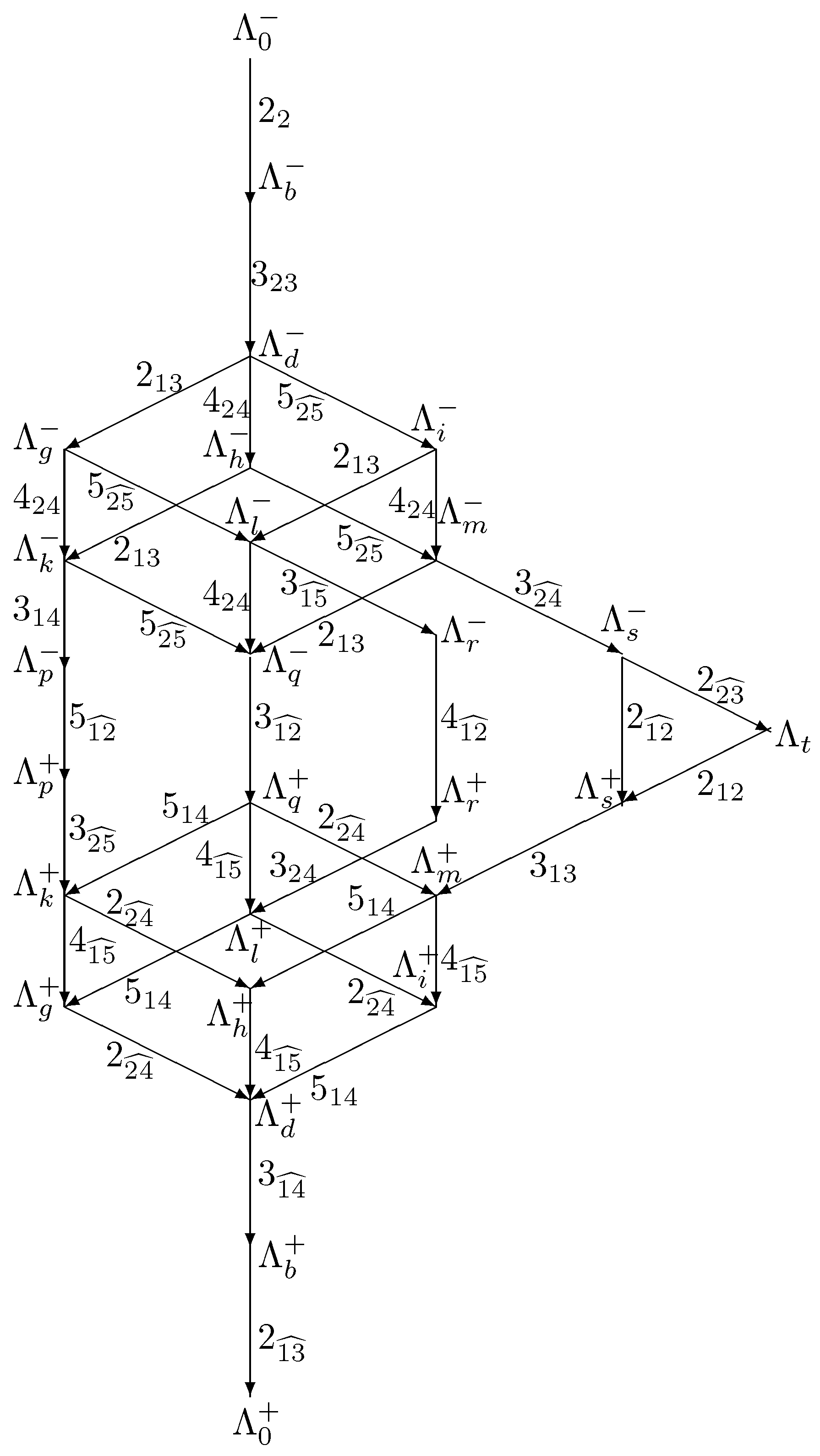
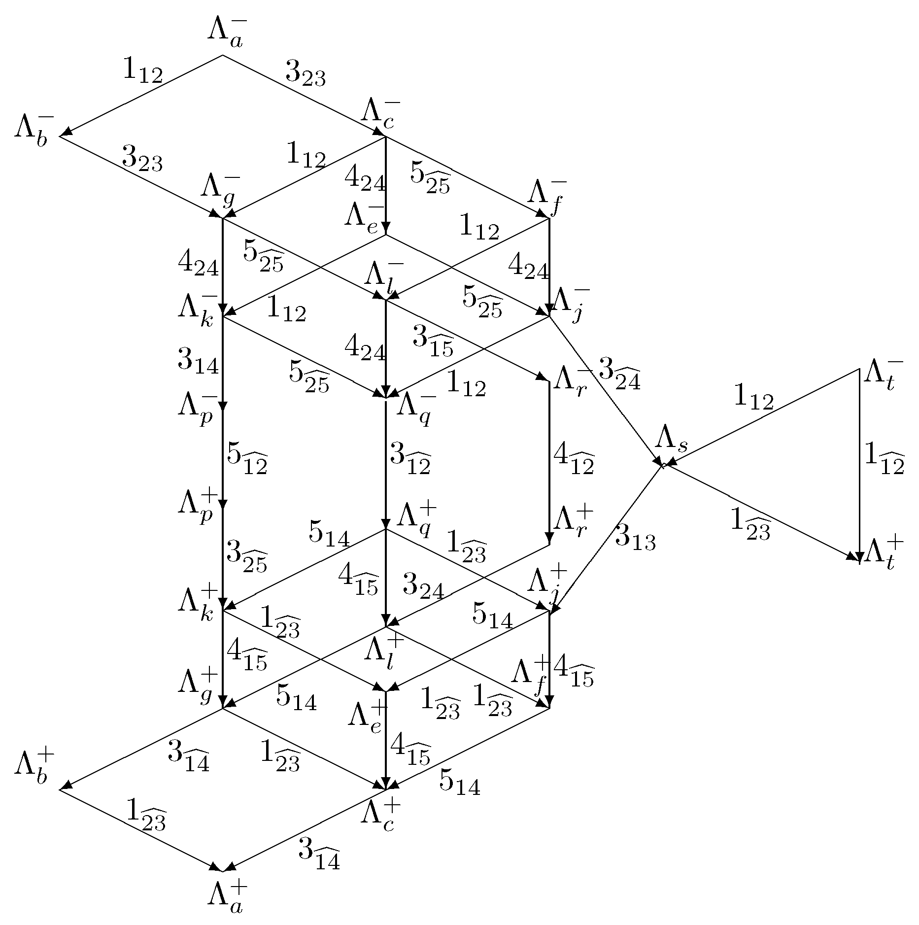
5. Reduced Multiplets

5.1. Main Reduced Multiplets

Intertwining differential operators occur not only in the main multiplets, but also in their reductions. There are five main reduced multiplets $M_k$, $k=1,2,3,4,5$, which may be obtained by setting the parameter $m_k=0$.

The main reduced multiplet $M_1$ contains 27 GVMs (ERs), see Figure 2. Their signatures are given as follows:

$$\begin{array}{ccc}\hfill {\chi }_0^{\pm }& =& \{0;m_3,m_4,m_5;\pm \frac{1}{2}{m}_{25,23}\}\hfill \\ \hfill {\chi }_b^{\pm }& =& \{m_2;m_{23},m_4,m_5;\pm \frac{1}{2}{m}_{25,3}\}={\chi }_a^{\pm }\hfill \\ \hfill {\chi }_d^{\pm }& =& \{m_{23};m_2,m_{34},m_{3,5};\pm \frac{1}{2}{m}_{25}\}={\chi }_c^{\pm }\hfill \\ \hfill {\chi }_g^{\pm }& =& \{m_3;0,m_{24},m_{23,5};\pm \frac{1}{2}{m}_{35}\}\hfill \\ \hfill {\chi }_h^{\pm }& =& \{m_{24};m_2,m_3,m_{35};\pm \frac{1}{2}{m}_{23,5}\}={\chi }_e^{\pm }\hfill \\ \hfill {\chi }_i^{\pm }& =& \{m_{23,5};m_2,m_{35},m_3;\pm \frac{1}{2}{m}_{24}\}={\chi }_f^{\pm }\hfill \\ \hfill {\chi }_k^{\pm }& =& \{m_{34};0,m_{23},m_{25};\pm \frac{1}{2}{m}_{3,5}\}\hfill \\ \hfill {\chi }_l^{\pm }& =& \{m_{3,5};0,m_{25},m_{23};\pm \frac{1}{2}{m}_{34}\}\hfill \\ \hfill {\chi }_m^{\pm }& =& \{m_{25};m_2,m_{3,5},m_{34};\pm \frac{1}{2}{m}_{23}\}={\chi }_j^{\pm }\hfill \\ \hfill {\chi }_p^{\pm }& =& \{m_4;0,m_2,m_{25,3};\pm \frac{1}{2}{m}_5\}\hfill \\ \hfill {\chi }_q^{\pm }& =& \{m_{35};0,m_{23,5},m_{24};\pm \frac{1}{2}{m}_3\}\hfill \\ \hfill {\chi }_r^{\pm }& =& \{m_5;0,m_{25,3},m_2;\pm \frac{1}{2}{m}_4\}\hfill \\ \hfill {\chi }_s^{\pm }& =& \{m_{25,3};m_{23},m_5,m_4;\pm \frac{1}{2}{m}_2\}={\chi }_n^{\pm }\hfill \\ \hfill {\chi }_t& =& \{m_{25,23};m_3,m_5,m_4;0\}\hfill \end{array}$$

Note that some of the inducing representations, namely, ${\chi }_0^{\pm }$, ${\chi }_g^{\pm }$, ${\chi }_k^{\pm }$, ${\chi }_l^{\pm }$, ${\chi }_p^{\pm }$, ${\chi }_q^{\pm }$, ${\chi }_r^{\pm }$, are limits of $\mathcal{M}$ representations, while the rest are finite-dimensional IRs (as in the main multiplets).

The main reduced multiplet $M_2$ contains 27 GVMs (ERs), see Figure 3, with signatures given as follows:

$$\begin{array}{ccc}\hfill {\chi }_0^{\pm }& =& \{m_1;m_3,m_4,m_5;\pm \frac{1}{2}{m}_{1,35,3}\}={\chi }_a^{\pm }\hfill \\ \hfill {\chi }_b^{\pm }& =& \{0;m_{1,3},m_4,m_5;\pm \frac{1}{2}{m}_{35,3}\}\hfill \\ \hfill {\chi }_c^{\pm }& =& \{m_{1,3};0,m_{34},m_{3,5};\pm \frac{1}{2}{m}_{1,35}\}\hfill \\ \hfill {\chi }_e^{\pm }& =& \{m_{1,34};0,m_3,m_{35};\pm \frac{1}{2}{m}_{1,3,5}\}\hfill \\ \hfill {\chi }_f^{\pm }& =& \{m_{1,3,5};0,m_{35},m_3;\pm \frac{1}{2}{m}_{1,34}\}\hfill \\ \hfill {\chi }_g^{\pm }& =& \{m_3;m_1,m_{34},m_{3,5};\pm \frac{1}{2}{m}_{35}\}={\chi }_d^{\pm }\hfill \\ \hfill {\chi }_j^{\pm }& =& \{m_{1,35};0,m_{3,5},m_{34};\pm \frac{1}{2}{m}_{1,3}\}\hfill \\ \hfill {\chi }_k^{\pm }& =& \{m_{34};m_1,m_3,m_{35};\pm \frac{1}{2}{m}_{3,5}\}={\chi }_h^{\pm }\hfill \\ \hfill {\chi }_l^{\pm }& =& \{m_{3,5};m_1,m_{35},m_3;\pm \frac{1}{2}{m}_{34}\}={\chi }_i^{\pm }\hfill \\ \hfill {\chi }_p^{\pm }& =& \{m_4;m_1,0,m_{35,3};\pm \frac{1}{2}{m}_5\}\hfill \\ \hfill {\chi }_q^{\pm }& =& \{m_{35};m_1,m_{3,5},m_{34};\pm \frac{1}{2}{m}_3\}={\chi }_m^{\pm }\hfill \\ \hfill {\chi }_r^{\pm }& =& \{m_5;m_1,m_{35,3},0;\pm \frac{1}{2}{m}_4\}\hfill \\ \hfill {\chi }_s& =& \{m_{35,3};m_{1,3},m_5,m_4;0\}\hfill \\ \hfill {\chi }_t^{\pm }& =& \{m_{1,35,3};m_3,m_5,m_4;\pm \frac{1}{2}{m}_1\}={\chi }_n^{\pm }\hfill \end{array}$$

(30)

The main reduced multiplet $M_3$ contains 27 GVMs (ERs), see Figure 4:

$$\begin{array}{ccc}\hfill {\chi }_0^{\pm }& =& \{m_1;0,m_4,m_5;\pm \frac{1}{2}{m}_{12,45,2}\}\hfill \\ \hfill {\chi }_c^{\pm }& =& \{m_{12};m_2,m_4,m_5;\pm \frac{1}{2}{m}_{12,45}\}={\chi }_a^{\pm }\hfill \\ \hfill {\chi }_d^{\pm }& =& \{m_2;m_{12},m_4,m_5;\pm \frac{1}{2}{m}_{2,45}\}={\chi }_b^{\pm }\hfill \\ \hfill {\chi }_e^{\pm }& =& \{m_{12,4};m_2,0,m_{45};\pm \frac{1}{2}{m}_{12,5}\}\hfill \\ \hfill {\chi }_f^{\pm }& =& \{m_{12,5};m_2,m_{45},0;\pm \frac{1}{2}{m}_{12,4}\}\hfill \\ \hfill {\chi }_g^{\pm }& =& \{0;m_1,m_{2,4},m_{2,5};\pm \frac{1}{2}{m}_{45}\}\hfill \\ \hfill {\chi }_h^{\pm }& =& \{m_{2,4};m_{12},0,m_{45};\pm \frac{1}{2}{m}_{2,5}\}\hfill \\ \hfill {\chi }_i^{\pm }& =& \{m_{2,5};m_{12},m_{45},0;\pm \frac{1}{2}{m}_{2,4}\}\hfill \\ \hfill {\chi }_j^{\pm }& =& \{m_{12,45};m_2,m_5,m_4;\pm \frac{1}{2}{m}_{12}\}={\chi }_n^{\pm }\hfill \\ \hfill {\chi }_k^{\pm }& =& \{m_4;m_1,m_2,m_{2,45};\pm \frac{1}{2}{m}_5\}={\chi }_p^{\pm }\hfill \\ \hfill {\chi }_l^{\pm }& =& \{m_5;m_1,m_{2,45},m_2;\pm \frac{1}{2}{m}_4\}={\chi }_r^{\pm }\hfill \\ \hfill {\chi }_m^{\pm }& =& \{m_{2,45};m_{12},m_5,m_4;\pm \frac{1}{2}{m}_2\}={\chi }_s^{\pm }\hfill \\ \hfill {\chi }_q& =& \{m_{45};m_1,m_{2,5},m_{2,4};0\}\hfill \\ \hfill {\chi }_t^{\pm }& =& \{m_{12,45,2};0,m_5,m_4;\pm \frac{1}{2}{m}_1\}\hfill \end{array}$$

The main reduced multiplet $M_4$ contains 27 GVMs (ERs), see Figure 5:

$$\begin{array}{ccc}\hfill {\chi }_0^{\pm }& =& \{m_1;m_3,0,m_5;\pm \frac{1}{2}{m}_{13,5,23}\}\hfill \\ \hfill {\chi }_a^{\pm }& =& \{m_{12};m_{23},0,m_5;\pm \frac{1}{2}{m}_{13,5,3}\}\hfill \\ \hfill {\chi }_b^{\pm }& =& \{m_2;m_{13},0,m_5;\pm \frac{1}{2}{m}_{23,5,3}\}\hfill \\ \hfill {\chi }_e^{\pm }& =& \{m_{13};m_2,m_3,m_{3,5};\pm \frac{1}{2}{m}_{13,5}\}={\chi }_c^{\pm }\hfill \\ \hfill {\chi }_h^{\pm }& =& \{m_{23};m_{12},m_3,m_{3,5};\pm \frac{1}{2}{m}_{23,5}\}={\chi }_d^{\pm }\hfill \\ \hfill {\chi }_j^{\pm }& =& \{m_{13,5};m_2,m_{3,5},m_3;\pm \frac{1}{2}{m}_{13}\}={\chi }_f^{\pm }\hfill \\ \hfill {\chi }_k^{\pm }& =& \{m_3;m_1,m_{23},m_{23,5};\pm \frac{1}{2}{m}_{3,5}\}={\chi }_g^{\pm }\hfill \\ \hfill {\chi }_m^{\pm }& =& \{m_{23,5};m_{12},m_{3,5},m_3;\pm \frac{1}{2}{m}_{23}\}={\chi }_i^{\pm }\hfill \\ \hfill {\chi }_n^{\pm }& =& \{m_{13,5,3};m_{23},m_5,0;\pm \frac{1}{2}{m}_{12}\}\hfill \\ \hfill {\chi }_p^{\pm }& =& \{0;m_1,m_2,m_{23,5,3};\pm \frac{1}{2}{m}_5\}\hfill \\ \hfill {\chi }_q^{\pm }& =& \{m_{3,5};m_1,m_{23,5},m_{23};\pm \frac{1}{2}{m}_3\}={\chi }_l^{\pm }\hfill \\ \hfill {\chi }_r& =& \{m_5;m_1,m_{23,5,3},m_2;0\}\hfill \\ \hfill {\chi }_s^{\pm }& =& \{m_{23,5,3};m_{13},m_5,0;\pm \frac{1}{2}{m}_2\}\hfill \\ \hfill {\chi }_t^{\pm }& =& \{m_{13,5,23};m_3,m_5,0;\pm \frac{1}{2}{m}_1\}\hfill \end{array}$$

(31)

The main reduced multiplet $M_5$ contains 27 GVMs (ERs), see Figure 6:

$$\begin{array}{ccc}\hfill {\chi }_0^{\pm }& =& \{m_1;m_3,m_4,0;\pm \frac{1}{2}{m}_{14,23}\}\hfill \\ \hfill {\chi }_a^{\pm }& =& \{m_{12};m_{23},m_4,0;\pm \frac{1}{2}{m}_{14,3}\}\hfill \\ \hfill {\chi }_b^{\pm }& =& \{m_2;m_{13},m_4,0;\pm \frac{1}{2}{m}_{24,3}\}\hfill \\ \hfill {\chi }_f^{\pm }& =& \{m_{13};m_2,m_{34},m_3;\pm \frac{1}{2}{m}_{14}\}={\chi }_c^{\pm }\hfill \\ \hfill {\chi }_i^{\pm }& =& \{m_{23};m_{12},m_{34},m_3;\pm \frac{1}{2}{m}_{24}\}={\chi }_d^{\pm }\hfill \\ \hfill {\chi }_j^{\pm }& =& \{m_{14};m_2,m_3,m_{34};\pm \frac{1}{2}{m}_{13}\}={\chi }_e^{\pm }\hfill \\ \hfill {\chi }_l^{\pm }& =& \{m_3;m_1,m_{24},m_{23};\pm \frac{1}{2}{m}_{34}\}={\chi }_g^{\pm }\hfill \\ \hfill {\chi }_m^{\pm }& =& \{m_{24};m_{12},m_3,m_{34};\pm \frac{1}{2}{m}_{23}\}={\chi }_h^{\pm }\hfill \\ \hfill {\chi }_n^{\pm }& =& \{m_{14,3};m_{23},0,m_4;\pm \frac{1}{2}{m}_{12}\}\hfill \\ \hfill {\chi }_p& =& \{m_4;m_1,m_2,m_{24,3};0\}\hfill \\ \hfill {\chi }_q^{\pm }& =& \{m_{34};m_1,m_{23},m_{24};\pm \frac{1}{2}{m}_3\}={\chi }_k^{\pm }\hfill \\ \hfill {\chi }_r^{\pm }& =& \{0;m_1,m_{24,3},m_2;\pm \frac{1}{2}{m}_4\}\hfill \\ \hfill {\chi }_s^{\pm }& =& \{m_{24,3};m_{13},0,m_4;\pm \frac{1}{2}{m}_2\}\hfill \\ \hfill {\chi }_t^{\pm }& =& \{m_{14,23};m_3,0,m_4;\pm \frac{1}{2}{m}_1\}\hfill \end{array}$$

(32)

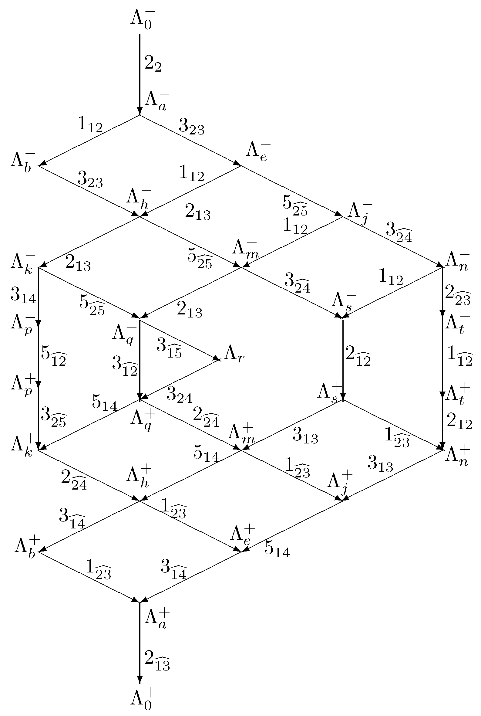
5.2. Next Reduced Multiplets

There are intertwining differential operators also in the next reduced multiplets. We start with cases $M_{ij}$ ($i<j$) when $m_i=m_j=0$.

The reduced multiplet $M_{12}$ contains 15 GVMs (ERs) with signatures given as follows:

$$\begin{array}{ccc}\hfill {\chi }_b^{\pm }& =& \{0;m_3,m_4,m_5;\pm \frac{1}{2}{m}_{35,3}\}={\chi }_a^{\pm }={\chi }_0^{\pm }\hfill \\ \hfill {\chi }_g^{\pm }& =& \{m_3;0,m_{34},m_{3,5};\pm \frac{1}{2}{m}_{35}\}={\chi }_c^{\pm }={\chi }_d^{\pm }\hfill \\ \hfill {\chi }_k^{\pm }& =& \{m_{34};0,m_3,m_{35};\pm \frac{1}{2}{m}_{3,5}\}={\chi }_e^{\pm }={\chi }_h^{\pm }\hfill \\ \hfill {\chi }_l^{\pm }& =& \{m_{3,5};0,m_{35},m_3;\pm \frac{1}{2}{m}_{34}\}={\chi }_i^{\pm }={\chi }_f^{\pm }\hfill \\ \hfill {\chi }_p^{\pm }& =& \{m_4;0,0,m_{35,3};\pm \frac{1}{2}{m}_5\}\hfill \\ \hfill {\chi }_q^{\pm }& =& \{m_{35};0,m_{3,5},m_{34};\pm \frac{1}{2}{m}_3\}={\chi }_j^{\pm }={\chi }_m^{\pm }\hfill \\ \hfill {\chi }_r^{\pm }& =& \{m_5;0,m_{35,3},0;\pm \frac{1}{2}{m}_4\}\hfill \\ \hfill {\chi }_s& =& \{m_{35,3};m_3,m_5,m_4;0\}={\chi }_n^{\pm }={\chi }_t\hfill \end{array}$$

Here we note only the ER ${\chi }_s$ which is induced from finite-dimensional $\mathcal{M}$-irrep, and where the subrepresentation is a singlet.

The reduced multiplet $M_{13}$ contains 18 GVMs (ERs):

$$\begin{array}{ccc}\hfill {\chi }_0^{\pm }& =& \{0;0,m_4,m_5;\pm \frac{1}{2}{m}_{2,45,2}\}\hfill \\ \hfill {\chi }_d^{\pm }& =& \{m_2;m_2,m_4,m_5;\pm \frac{1}{2}{m}_{2,45}\}={\chi }_b^{\pm }\hfill \\ \hfill {\chi }_g^{\pm }& =& \{0;0,m_{2,4},m_{2,5};\pm \frac{1}{2}{m}_{45}\}\hfill \\ \hfill {\chi }_h^{\pm }& =& \{m_{2,4};m_2,0,m_{45};\pm \frac{1}{2}{m}_{2,5}\}={\chi }_e^{\pm }\hfill \\ \hfill {\chi }_i^{\pm }& =& \{m_{2,5};m_2,m_{45},0;\pm \frac{1}{2}{m}_{2,4}\}={\chi }_f^{\pm }\hfill \\ \hfill {\chi }_k^{\pm }& =& \{m_4;0,m_2,m_{2,45};\pm \frac{1}{2}{m}_5\}={\chi }_p^{\pm }\hfill \\ \hfill {\chi }_l^{\pm }& =& \{m_5;0,m_{2,45},m_2;\pm \frac{1}{2}{m}_4\}={\chi }_r^{\pm }\hfill \\ \hfill {\chi }_m^{\pm }& =& \{m_{2,45};m_2,m_5,m_4;\pm \frac{1}{2}{m}_2\}={\chi }_s^{\pm }\hfill \\ \hfill {\chi }_q& =& \{m_{45};0,m_{2,5},m_{2,4};0\}\hfill \\ \hfill {\chi }_t& =& \{m_{2,45,2};0,m_5,m_4;0\}\hfill \end{array}$$

Here we note the ERs ${\chi }_h^{\pm }$, ${\chi }_m^{\pm }$ induced from finite-dimensional $\mathcal{M}$-irreps, which doublets are related by KS operators, yet for the pair ${\mathsf{\Lambda }}_m^{\pm }$ the KS operator $G^{+}$ is actually the differential operator ${\mathcal{D}}_{m_3{\alpha }_{\widehat{12}}}$ .

The reduced multiplet $M_{14}$ contains 18 GVMs (ERs):

$$\begin{array}{ccc}\hfill {\chi }_0^{\pm }& =& \{0;m_3,0,m_5;\pm \frac{1}{2}{m}_{23,5,23}\}\hfill \\ \hfill {\chi }_b^{\pm }& =& \{m_2;m_{23},0,m_5;\pm \frac{1}{2}{m}_{23,5,3}\}={\chi }_a^{\pm }\hfill \\ \hfill {\chi }_h^{\pm }& =& \{m_{23};m_2,m_3,m_{3,5};\pm \frac{1}{2}{m}_{23,5}\}={\chi }_e^{\pm }={\chi }_c^{\pm }={\chi }_d^{\pm }\hfill \\ \hfill {\chi }_k^{\pm }& =& \{m_3;0,m_{23},m_{23,5};\pm \frac{1}{2}{m}_{3,5}\}={\chi }_g^{\pm }\hfill \\ \hfill {\chi }_m^{\pm }& =& \{m_{23,5};m_2,m_{3,5},m_3;\pm \frac{1}{2}{m}_{23}\}={\chi }_j^{\pm }={\chi }_i^{\pm }={\chi }_f^{\pm }\hfill \\ \hfill {\chi }_p^{\pm }& =& \{0;0,m_2,m_{23,5,3};\pm \frac{1}{2}{m}_5\}\hfill \\ \hfill {\chi }_q^{\pm }& =& \{m_{3,5};0,m_{23,5},m_{23};\pm \frac{1}{2}{m}_3\}={\chi }_l^{\pm }\hfill \\ \hfill {\chi }_r& =& \{m_5;0,m_{23,5,3},m_2;0\}\hfill \\ \hfill {\chi }_s^{\pm }& =& \{m_{23,5,3};m_{23},m_5,0;\pm \frac{1}{2}{m}_2\}={\chi }_n^{\pm }\hfill \\ \hfill {\chi }_t& =& \{m_{23,5,23};m_3,m_5,0;0\}\hfill \end{array}$$

Here we note the ERs ${\chi }_h^{\pm }$, ${\chi }_m^{\pm }$ induced from finite-dimensional $\mathcal{M}$-irreps, and forming a sub-multiplet as follows:

$$\begin{array}{ccc}{\chi }_h^{-}& \genfrac{}{}{0pt}{}{{\mathcal{D}}_{\widehat{25}}^{m_5}}{⟶}& {\chi }_m^{-}\\ & & \\ \updownarrow & & \updownarrow \\ & & \\ {\chi }_h^{+}& \genfrac{}{}{0pt}{}{{\mathcal{D}}_{\widehat{25}}^{m_5}}{⟵}& {\chi }_m^{+}\end{array}$$

(33)

where the up-down arrows designate the KS operators.

The reduced multiplet $M_{15}$ contains 18 GVMs (ERs):

$$\begin{array}{ccc}\hfill {\chi }_0^{\pm }& =& \{0;m_3,m_4,0;\pm \frac{1}{2}{m}_{24,23}\}\hfill \\ \hfill {\chi }_b^{\pm }& =& \{m_2;m_{23},m_4,0;\pm \frac{1}{2}{m}_{24,3}\}={\chi }_a^{\pm }\hfill \\ \hfill {\chi }_i^{\pm }& =& \{m_{23};m_2,m_{34},m_3;\pm \frac{1}{2}{m}_{24}\}={\chi }_f^{\pm }={\chi }_d^{\pm }={\chi }_c^{\pm }\hfill \\ \hfill {\chi }_l^{\pm }& =& \{m_3;0,m_{24},m_{23};\pm \frac{1}{2}{m}_{34}\}={\chi }_g^{\pm }\hfill \\ \hfill {\chi }_m^{\pm }& =& \{m_{24};m_2,m_3,m_{34};\pm \frac{1}{2}{m}_{23}\}={\chi }_j^{\pm }={\chi }_h^{\pm }={\chi }_e^{\pm }\hfill \\ \hfill {\chi }_p& =& \{m_4;0,m_2,m_{24,3};0\}\hfill \\ \hfill {\chi }_q^{\pm }& =& \{m_{34};0,m_{23},m_{24};\pm \frac{1}{2}{m}_3\}={\chi }_k^{\pm }\hfill \\ \hfill {\chi }_r^{\pm }& =& \{0;0,m_{24,3},m_2;\pm \frac{1}{2}{m}_4\}\hfill \\ \hfill {\chi }_s^{\pm }& =& \{m_{24,3};m_{23},0,m_4;\pm \frac{1}{2}{m}_2\}={\chi }_n^{\pm }\hfill \\ \hfill {\chi }_t& =& \{m_{24,23};m_3,0,m_4;0\}\hfill \end{array}$$

Here we note the ERs ${\chi }_i^{\pm }$, ${\chi }_m^{\pm }$ induced from finite-dimensional $\mathcal{M}$-irreps, and forming a sub-multiplet as follows:

$$\begin{array}{ccc}{\chi }_i^{-}& \genfrac{}{}{0pt}{}{{\mathcal{D}}_{\widehat{24}}^{m_4}}{⟶}& {\chi }_m^{-}\\ & & \\ \updownarrow & & \updownarrow \\ & & \\ {\chi }_i^{+}& \genfrac{}{}{0pt}{}{{\mathcal{D}}_{\widehat{24}}^{m_4}}{⟵}& {\chi }_m^{+}\end{array}$$

(34)

The reduced multiplet $M_{23}$ contains 15 GVMs (ERs):

$$\begin{array}{ccc}\hfill {\chi }_c^{\pm }& =& \{m_1;0,m_4,m_5;\pm \frac{1}{2}{m}_{1,45}\}={\chi }_a^{\pm }={\chi }_0^{\pm }\hfill \\ \hfill {\chi }_e^{\pm }& =& \{m_{14};0,0,m_{45};\pm \frac{1}{2}{m}_{1,5}\}\hfill \\ \hfill {\chi }_f^{\pm }& =& \{m_{1,5};0,m_{45},0;\pm \frac{1}{2}{m}_{14}\}\hfill \\ \hfill {\chi }_g^{\pm }& =& \{0;m_1,m_4,m_5;\pm \frac{1}{2}{m}_{45}\}={\chi }_b^{\pm }={\chi }_d^{\pm }\hfill \\ \hfill {\chi }_j^{\pm }& =& \{m_{1,45};0,m_5,m_4;\pm \frac{1}{2}{m}_1\}={\chi }_t^{\pm }={\chi }_n^{\pm }\hfill \\ \hfill {\chi }_k^{\pm }& =& \{m_4;m_1,0,m_{45};\pm \frac{1}{2}{m}_5\}={\chi }_p^{\pm }={\chi }_h^{\pm }\hfill \\ \hfill {\chi }_l^{\pm }& =& \{m_5;m_1,m_{45},0;\pm \frac{1}{2}{m}_4\}={\chi }_r^{\pm }={\chi }_i^{\pm }\hfill \\ \hfill {\chi }_q& =& \{m_{45};m_1,m_5,m_4;0\}={\chi }_s={\chi }_m^{\pm }\hfill \end{array}$$

Here we note only the ER ${\chi }_q$ which is induced from finite-dimensional $\mathcal{M}$-irrep, and where the subrepresentation is a singlet.

The reduced multiplet $M_{24}$ contains 18 GVMs (ERs):

$$\begin{array}{ccc}\hfill {\chi }_0^{\pm }& =& \{m_1;m_3,0,m_5;\pm \frac{1}{2}{m}_{1,3,5,3}\}={\chi }_a^{\pm }\hfill \\ \hfill {\chi }_b^{\pm }& =& \{0;m_{1,3},0,m_5;\pm \frac{1}{2}{m}_{3,5,3}\}\hfill \\ \hfill {\chi }_e^{\pm }& =& \{m_{1,3};0,m_3,m_{3,5};\pm \frac{1}{2}{m}_{1,3,5}\}={\chi }_c^{\pm }\hfill \\ \hfill {\chi }_j^{\pm }& =& \{m_{1,3,5};0,m_{3,5},m_3;\pm \frac{1}{2}{m}_{1,3}\}={\chi }_f^{\pm }\hfill \\ \hfill {\chi }_h^{\pm }& =& \{m_3;m_1,m_3,m_{3,5};\pm \frac{1}{2}{m}_{3,5}\}={\chi }_g^{\pm }={\chi }_k^{\pm }={\chi }_d^{\pm }\hfill \\ \hfill {\chi }_p^{\pm }& =& \{0;m_1,0,m_{3,5,3};\pm \frac{1}{2}{m}_5\}\hfill \\ \hfill {\chi }_m^{\pm }& =& \{m_{3,5};m_1,m_{3,5},m_3;\pm \frac{1}{2}{m}_3\}={\chi }_l^{\pm }={\chi }_q^{\pm }={\chi }_i^{\pm }\hfill \\ \hfill {\chi }_r& =& \{m_5;m_1,m_{3,5,3},0;0\}\hfill \\ \hfill {\chi }_s& =& \{m_{3,5,3};m_{1,3},m_5,0;0\}\hfill \\ \hfill {\chi }_t^{\pm }& =& \{m_{1,3,5,3};m_3,m_5,0;\pm \frac{1}{2}{m}_1\}={\chi }_n^{\pm }\hfill \end{array}$$

Here we note the ERs ${\chi }_h^{\pm }$, ${\chi }_m^{\pm }$ induced from finite-dimensional $\mathcal{M}$-irreps, and forming a sub-multiplet as follows:

$$\begin{array}{ccc}{\chi }_h^{-}& \genfrac{}{}{0pt}{}{{\mathcal{D}}_{\widehat{25}}^{m_5}}{⟶}& {\chi }_m^{-}\\ & & \\ \updownarrow & & \uparrow \downarrow {\mathcal{D}}_{\widehat{12}}^{m_3}\\ & & \\ {\chi }_h^{+}& \genfrac{}{}{0pt}{}{{\mathcal{D}}_{\widehat{25}}^{m_5}}{⟵}& {\chi }_m^{+}\end{array}$$

(35)

where on the right a KS operator $G_{KS}^{+}$ is degenerated in the intertwining differential operator ${\mathcal{D}}_{\widehat{12}}^{m_3}$.

The reduced multiplet $M_{25}$ contains 18 GVMs (ERs) with signatures:

$$\begin{array}{ccc}\hfill {\chi }_0^{\pm }& =& \{m_1;m_3,m_4,0;\pm \frac{1}{2}{m}_{1,34,3}\}={\chi }_a^{\pm }\hfill \\ \hfill {\chi }_b^{\pm }& =& \{0;m_{1,3},m_4,0;\pm \frac{1}{2}{m}_{34,3}\}\hfill \\ \hfill {\chi }_f^{\pm }& =& \{m_{1,3};0,m_{34},m_3;\pm \frac{1}{2}{m}_{1,34}\}={\chi }_c^{\pm }\hfill \\ \hfill {\chi }_j^{\pm }& =& \{m_{1,34};0,m_3,m_{34};\pm \frac{1}{2}{m}_{1,3}\}={\chi }_e^{\pm }\hfill \\ \hfill {\chi }_l^{\pm }& =& \{m_3;m_1,m_{34},m_3;\pm \frac{1}{2}{m}_{34}\}={\chi }_g^{\pm }={\chi }_i^{\pm }={\chi }_d^{\pm }\hfill \\ \hfill {\chi }_p& =& \{m_4;m_1,0,m_{34,3};0\}\hfill \\ \hfill {\chi }_m^{\pm }& =& \{m_{34};m_1,m_3,m_{34};\pm \frac{1}{2}{m}_3\}={\chi }_k^{\pm }={\chi }_q^{\pm }={\chi }_h^{\pm }\hfill \\ \hfill {\chi }_r^{\pm }& =& \{0;m_1,m_{34,3},0;\pm \frac{1}{2}{m}_4\}\hfill \\ \hfill {\chi }_s& =& \{m_{34,3};m_{1,3},0,m_4;0\}\hfill \\ \hfill {\chi }_t^{\pm }& =& \{m_{1,34,3};m_3,0,m_4;\pm \frac{1}{2}{m}_1\}={\chi }_n^{\pm }\hfill \end{array}$$

Here we note the ERs ${\chi }_l^{\pm }$, ${\chi }_m^{\pm }$ induced from finite-dimensional $\mathcal{M}$-irreps, and forming a sub-multiplet as follows:

$$\begin{array}{ccc}{\chi }_l^{-}& \genfrac{}{}{0pt}{}{{\mathcal{D}}_{\widehat{24}}^{m_4}}{⟶}& {\chi }_m^{-}\\ & & \\ \updownarrow & & \uparrow \downarrow {\mathcal{D}}_{\widehat{12}}^{m_3}\\ & & \\ {\chi }_i^{+}& \genfrac{}{}{0pt}{}{{\mathcal{D}}_{\widehat{25}}^{m_5}}{⟵}& {\chi }_m^{+}\end{array}$$

(36)

The reduced multiplet $M_{34}$ contains 15 GVMs (ERs):

$$\begin{array}{ccc}\hfill {\chi }_0^{\pm }& =& \{m_1;0,0,m_5;\pm \frac{1}{2}{m}_{12,5,2}\}\hfill \\ \hfill {\chi }_c^{\pm }& =& \{m_{12};m_2,0,m_5;\pm \frac{1}{2}{m}_{12,5}\}={\chi }_e^{\pm }={\chi }_a^{\pm }\hfill \\ \hfill {\chi }_d^{\pm }& =& \{m_2;m_{12},0,m_5;\pm \frac{1}{2}{m}_{2,5}\}={\chi }_h^{\pm }={\chi }_b^{\pm }\hfill \\ \hfill {\chi }_j^{\pm }& =& \{m_{12,5};m_2,m_5,0;\pm \frac{1}{2}{m}_{12}\}={\chi }_f^{\pm }={\chi }_n^{\pm }\hfill \\ \hfill {\chi }_k^{\pm }& =& \{0;m_1,m_2,m_{2,5};\pm \frac{1}{2}{m}_5\}={\chi }_g^{\pm }={\chi }_p^{\pm }\hfill \\ \hfill {\chi }_l& =& \{m_5;m_1,m_{2,5},m_2;0\}={\chi }_q={\chi }_r^{\pm }\hfill \\ \hfill {\chi }_m^{\pm }& =& \{m_{2,5};m_{12},m_5,0;\pm \frac{1}{2}{m}_2\}={\chi }_i^{\pm }={\chi }_s^{\pm }\hfill \\ \hfill {\chi }_t^{\pm }& =& \{m_{12,5,2};0,m_5,0;\pm \frac{1}{2}{m}_1\}\hfill \end{array}$$

Here we note only the ER ${\chi }_l$ which is induced from finite-dimensional $\mathcal{M}$-irrep, and where the subrepresentation is a singlet.

The reduced multiplet $M_{35}$ contains 15 GVMs (ERs):

$$\begin{array}{ccc}\hfill {\chi }_0^{\pm }& =& \{m_1;0,m_4,0;\pm \frac{1}{2}{m}_{12,4,2}\}\hfill \\ \hfill {\chi }_c^{\pm }& =& \{m_{12};m_2,m_4,0;\pm \frac{1}{2}{m}_{12,4}\}={\chi }_f^{\pm }={\chi }_a^{\pm }\hfill \\ \hfill {\chi }_d^{\pm }& =& \{m_2;m_{12},m_4,0;\pm \frac{1}{2}{m}_{2,4}\}={\chi }_i^{\pm }={\chi }_b^{\pm }\hfill \\ \hfill {\chi }_j^{\pm }& =& \{m_{12,4};m_2,0,m_4;\pm \frac{1}{2}{m}_{12}\}={\chi }_e^{\pm }={\chi }_n^{\pm }\hfill \\ \hfill {\chi }_k& =& \{m_4;m_1,m_2,m_{2,4};0\}={\chi }_q={\chi }_p^{\pm }\hfill \\ \hfill {\chi }_l^{\pm }& =& \{0;m_1,m_{2,4},m_2;\pm \frac{1}{2}{m}_4\}={\chi }_g^{\pm }={\chi }_r^{\pm }\hfill \\ \hfill {\chi }_m^{\pm }& =& \{m_{2,4};m_{12},0,m_4;\pm \frac{1}{2}{m}_2\}={\chi }_h^{\pm }={\chi }_s^{\pm }\hfill \\ \hfill {\chi }_t^{\pm }& =& \{m_{12,4,2};0,0,m_4;\pm \frac{1}{2}{m}_1\}\hfill \end{array}$$

Here we note only the ER ${\chi }_k$ which is induced from finite-dimensional $\mathcal{M}$-irrep, and where the subrepresentation is a singlet.

The reduced multiplet $M_{45}$ contains 20 GVMs (ERs):

$$\begin{array}{ccc}\hfill {\chi }_0^{\pm }& =& \{m_1;m_3,0,0;\pm \frac{1}{2}{m}_{13,23}\}\hfill \\ \hfill {\chi }_a^{\pm }& =& \{m_{12};m_{23},0,0;\pm \frac{1}{2}{m}_{13,3}\}\hfill \\ \hfill {\chi }_b^{\pm }& =& \{m_2;m_{13},0,0;\pm \frac{1}{2}{m}_{23,3}\}\hfill \\ \hfill {\chi }_j^{\pm }& =& \{m_{13};m_2,m_3,m_3;\pm \frac{1}{2}{m}_{13}\}={\chi }_e^{\pm }={\chi }_f^{\pm }={\chi }_c^{\pm }\hfill \\ \hfill {\chi }_m^{\pm }& =& \{m_{23};m_{12},m_3,m_3;\pm \frac{1}{2}{m}_{23}\}={\chi }_h^{\pm }={\chi }_i^{\pm }={\chi }_d^{\pm }\hfill \\ \hfill {\chi }_n^{\pm }& =& \{m_{13,3};m_{23},0,0;\pm \frac{1}{2}{m}_{12}\}\hfill \\ \hfill {\chi }_p& =& \{0;m_1,m_2,m_{23,3};0\}\hfill \\ \hfill {\chi }_q^{\pm }& =& \{m_3;m_1,m_{23},m_{23};\pm \frac{1}{2}{m}_3\}={\chi }_k^{\pm }={\chi }_l^{\pm }={\chi }_g^{\pm }\hfill \\ \hfill {\chi }_r& =& \{0;m_1,m_{23,3},m_2;0\}\hfill \\ \hfill {\chi }_s^{\pm }& =& \{m_{23,3};m_{13},0,0;\pm \frac{1}{2}{m}_2\}\hfill \\ \hfill {\chi }_t^{\pm }& =& \{m_{13,23};m_3,0,0;\pm \frac{1}{2}{m}_1\}\hfill \end{array}$$

Here we note the ERs ${\chi }_j^{\pm }$, ${\chi }_m^{\pm }$, ${\chi }_q^{\pm }$, induced from finite-dimensional $\mathcal{M}$-irreps, and forming a sub-multiplet as follows:

$$\begin{array}{ccccc}{\chi }_j^{-}& \genfrac{}{}{0pt}{}{{\mathcal{D}}_{12}^{m_1}}{⟶}& {\chi }_m^{-}& \genfrac{}{}{0pt}{}{{\mathcal{D}}_{13}^{m_2}}{⟶}& {\chi }_q^{-}\\ & & & & \\ \updownarrow & & \updownarrow & & \uparrow \downarrow {\mathcal{D}}_{\widehat{12}}^{m_3}\\ & & & & \\ {\chi }_j^{+}& \genfrac{}{}{0pt}{}{{\mathcal{D}}_{\widehat{13}}^{m_1}}{⟵}& {\chi }_m^{+}& \genfrac{}{}{0pt}{}{{\mathcal{D}}_{\widehat{24}}^{m_2}}{⟵}& {\chi }_m^{+}\end{array}$$

(37)

5.3. Third Level Reduction of Multiplets

In the next levels of reductions, there are only two multiplets containing ERs induced from finite-dimensional $\mathcal{M}$-irreps, actually, each contains a doublet related by KS operators:

The reduced multiplet $M_{145}$ contains 13 GVMs (ERs):

$$\begin{array}{ccc}\hfill {\chi }_0^{\pm }& =& \{0;m_3,0,0;\pm \frac{1}{2}{m}_{23,23}\}\hfill \\ \hfill {\chi }_b^{\pm }& =& \{m_2;m_{23},0,0;\pm \frac{1}{2}{m}_{23,3}\}={\chi }_a^{\pm }\hfill \\ \hfill {\chi }_m^{\pm }& =& \{m_{23};m_2,m_3,m_3;\pm \frac{1}{2}{m}_{23}\}={\chi }_h^{\pm }={\chi }_j^{\pm }={\chi }_i^{\pm }={\chi }_f^{\pm }={\chi }_e^{\pm }={\chi }_c^{\pm }={\chi }_d^{\pm }\hfill \\ \hfill {\chi }_p& =& \{0;0,m_2,m_{23,3};0\}\hfill \\ \hfill {\chi }_q^{\pm }& =& \{m_3;0,m_{23},m_{23};\pm \frac{1}{2}{m}_3\}={\chi }_k^{\pm }={\chi }_l^{\pm }={\chi }_g^{\pm }\hfill \\ \hfill {\chi }_r& =& \{0;0,m_{23,3},m_2;0\}\hfill \\ \hfill {\chi }_s^{\pm }& =& \{m_{23,3};m_{23},0,0;\pm \frac{1}{2}{m}_2\}={\chi }_n^{\pm }\hfill \\ \hfill {\chi }_t& =& \{m_{23,23};m_3,0,0;0\}\hfill \end{array}$$

The relevant doublet is ${\chi }_m^{\pm }$.

The reduced multiplet $M_{245}$ contains 13 GVMs (ERs):

$$\begin{array}{ccc}\hfill {\chi }_0^{\pm }& =& \{m_1;m_3,0,0;\pm \frac{1}{2}{m}_{1,3,3}\}={\chi }_a^{\pm }\hfill \\ \hfill {\chi }_b^{\pm }& =& \{0;m_{1,3},0,0;\pm \frac{1}{2}{m}_{3,3}\}\hfill \\ \hfill {\chi }_j^{\pm }& =& \{m_{1,3};0,m_3,m_3;\pm \frac{1}{2}{m}_{1,3}\}={\chi }_e^{\pm }={\chi }_f^{\pm }={\chi }_c^{\pm }\hfill \\ \hfill {\chi }_p& =& \{0;m_1,0,m_{3,3};0\}\hfill \\ \hfill {\chi }_q^{\pm }& =& \{m_3;m_1,m_3,m_3;\pm \frac{1}{2}{m}_3\}={\chi }_k^{\pm }={\chi }_l^{\pm }={\chi }_m^{\pm }={\chi }_i^{\pm }={\chi }_g^{\pm }={\chi }_h^{\pm }={\chi }_d^{\pm }\hfill \\ \hfill {\chi }_r& =& \{0;m_1,m_{3,3},0;0\}\hfill \\ \hfill {\chi }_s& =& \{m_{3,3};m_{1,3},0,0;0\}\hfill \\ \hfill {\chi }_t^{\pm }& =& \{m_{1,3,3};m_3,0,0;\pm \frac{1}{2}{m}_1\}={\chi }_n^{\pm }\hfill \end{array}$$

The relevant doublet is ${\chi }_q^{\pm }$ where the KS operator $G_{KS}^{+}$ degenerates to the intertwining differential operator ${\mathcal{D}}_{\widehat{12}}^{m_3}$.

References

- Dobrev, V.K. Invariant differential operators for non-compact Lie groups: Parabolic subalgebras. Rev. Math. Phys. 2008, 20, 407–449. [Google Scholar] [CrossRef] [Green Version]
- Dobrev, V.K. Invariant Differential Operators, Volume 1: Noncompact Semisimple Lie Algebras and Groups; De Gruyter Studies in Mathematical Physics; De Gruyter: Berlin, Germany; Boston, MA, USA, 2016; Volume 35, p. 408. ISBN 978-3-11-042764-6. [Google Scholar]
- Dobrev, V.K. Invariant differential operators for non-compact Lie algebras parabolically related to conformal Lie algebras. J. High Energy Phys. 2013, 2, 015. [Google Scholar] [CrossRef] [Green Version]
- Langlands, R.P. On the Classification of Irreducible Representations of Real Algebraic Groups. Math. Surv. Monographs 1988, 31, 101–170, first as IAS Princeton preprint, 1973. [Google Scholar]
- Zhelobenko, D.P. Harmonic Analysis on Semisimple Complex Lie Groups; Nauka: Moscow, Russia, 1974. (In Russian) [Google Scholar]
- Knapp, A.W.; Zuckerman, G.J. Classification Theorems for Representations of Semisimple Groups; Lecture Notes in Math; Springer: Berlin, Germany, 1977; Volume 587, pp. 138–159. [Google Scholar]
- Knapp, A.W.; Zuckerman, G.J. Classification of irreducible tempered representations of semisimple groups. Ann. Math. 1982, 16, 389–501. [Google Scholar] [CrossRef]
- Dobrev, V.K.; Mack, G.; Petkova, V.B.; Petrova, S.G.; Todorov, I.T. On the Clebsch-Gordan expansion for the Lorentz group in n dimensions. Rept. Math. Phys. 1976, 9, 219–246. [Google Scholar] [CrossRef]
- Dobrev, V.K.; Mack, G.; Petkova, V.B.; Petrova, S.G.; Todorov, I.T. Harmonic Analysis on the n-Dimensional Lorentz Group and Its Applications to Conformal Quantum Field Theory; Lecture Notes in Physics; Springer: Berlin, Germany, 1977. [Google Scholar]
- Harish-Chandra, B. Discrete series for semisimple Lie groups II. Acta Math. 1966, 116, 1–111. [Google Scholar] [CrossRef]
- Dobrev, V.K. Canonical construction of differential operators intertwining representations of real semisimple Lie groups. Rept. Math. Phys. 1988, 25, 159–181, first as ICTP Trieste preprint IC/86/393 (1986). [Google Scholar] [CrossRef]
- Dobrev, V.K. Multiplet classification of the reducible elementary representations of real semisimple Lie groups: The SO e (p, q) example. Lett. Math. Phys. 1985, 9, 205–211. [Google Scholar] [CrossRef]
- Bernstein, I.N.; Gel’fand, I.M.; Gel’fand, S.I. Structure of representations generated by vectors of highest weight. Funkts. Anal. Prilozh. 1971, 5, 1–9, English translation: Funct. Anal. Appl. 1971, 5, 1–8. [Google Scholar] [CrossRef]
- Dixmier, J. Enveloping Algebras; North Holland: New York, NY, USA, 1977. [Google Scholar]
- Knapp, A.W.; Stein, E.M. Interwining operators for semisimple groups. Ann. Math. 1971, 93, 489–578. [Google Scholar] [CrossRef]
- Knapp, A.W.; Stein, E.M. Intertwining operators for semisimple groups, II. Inv. Math. 1980, 60, 9–84. [Google Scholar] [CrossRef]
Publisher’s Note: MDPI stays neutral with regard to jurisdictional claims in published maps and institutional affiliations. |
© 2022 by the author. Licensee MDPI, Basel, Switzerland. This article is an open access article distributed under the terms and conditions of the Creative Commons Attribution (CC BY) license (https://creativecommons.org/licenses/by/4.0/).
Share and Cite
Dobrev, V.K. Heisenberg Parabolic Subgroup of SO∗(10) and Invariant Differential Operators. Symmetry 2022, 14, 1592. https://doi.org/10.3390/sym14081592
Dobrev VK. Heisenberg Parabolic Subgroup of SO∗(10) and Invariant Differential Operators. Symmetry. 2022; 14(8):1592. https://doi.org/10.3390/sym14081592
Chicago/Turabian StyleDobrev, V. K. 2022. "Heisenberg Parabolic Subgroup of SO∗(10) and Invariant Differential Operators" Symmetry 14, no. 8: 1592. https://doi.org/10.3390/sym14081592
APA StyleDobrev, V. K. (2022). Heisenberg Parabolic Subgroup of SO∗(10) and Invariant Differential Operators. Symmetry, 14(8), 1592. https://doi.org/10.3390/sym14081592