A New Solvable Generalized Trigonometric Tangent Potential Based on SUSYQM

Abstract

Supersymmetric quantum mechanics has wide applications in physics. However, there are few potentials that can be solved exactly by supersymmetric quantum mechanics methods, so it is undoubtedly of great significance to find more potentials that can be solved exactly. This paper studies the supersymmetric quantum mechanics problems of the Schrödinger equation with a new kind of generalized trigonometric tangent superpotential: $A\tan npx+B\tan mpx$. We will elaborate on this new potential in the following aspects. Firstly, the shape invariant relation of partner potential is generated by the generalized trigonometric tangent superpotential. We find three shape invariance forms that satisfy the additive condition. Secondly, the eigenvalues and the eigenwave functions of the potential are studied separately in these three cases. Thirdly, the potential algebra of such a superpotential is discussed, and the discussions are explored from two aspects: one parameter’s and two parameters’ potential algebra. Through the potential algebra, the eigenvalue spectrums are given separately which are consistent with those mentioned earlier. Finally, we summarize the paper and give an outlook on the two-parameter shape-invariant potential.

1. Introduction

The concept of Supersymmetry (SUSY) has permeated almost all fields of Physics: atomic and molecular physics, nuclear physics, statistical physics, and condensed matter physics [1,2,3,4]. It is even considered a necessary way to establish any unified theory [5,6]. Although SUSY has achieved great success in theoretical physics, there has been no conclusive evidence of supersymmetric partners in experiments. It was introduced by Nicolai and Witten in non-relativistic quantum mechanics [7,8]. These researchers soon found that supersymmetric quantum mechanics (SUSYQM)was of great significance and soon became a method to solve the Schrödinger equation [3,4,9,10].

The exact or quasi-exact solution of the Schrödinger equation under various potential constraints has always been a particular concern in quantum mechanics [10,11,12,13,14]. There are only a dozen potentials which are solvable in Schrödinger equation through SUSYQM methods. These potentials mainly include harmonic oscillator potential, Coulomb potential, Morse potential, Rosen–Morse potential, Scarf potential, Eckart potential, Pösch–Teller potential, and so on [3,14,15,16,17,18,19,20,21,22,23]. Recently, the list of these potentials has been expanded [24,25,26]. These precisely solvable potentials also satisfy the shape invariance condition [3,27,28], and it is found that there is a deep connection between shape invariance and SUSY. These connections need to be dealt with from the perspective of group theory. The Lie algebra is an important part of the group theory, and the potential algebra theory allows for a deep analysis of SUSYQM [29,30,31,32]. The shape invariant potentials mentioned above naturally have corresponding potential algebraic forms. Therefore, it is undoubtedly of great significance to obtain the potential algebraic form of shape invariance. The above discussion leads to the following problems: (1) How to find more solvable potentials. (2) The Riccati equation satisfied from the superpotential is only a first-order differential equation, but the solution of the equation is not easy to obtain [33]. The known solvable potential and its superpotential are consistent. Therefore, how to find more solutions to the Ricati equations is also an important problem. (3) If we can construct more solvable potentials, what exciting new results will come from these new solvable potentials?

Our group has begun tryingto promote this research from the existing superpotential. The study in [26] is our first generalization, extending the hyperbolic tangent superpotential to a linear combination of two different hyperbolic tangent, bringing positive and meaningful results. The present paper is another attempted generalization, taking the linear combination of two tangent superpotentials as our generalization potential, and the results are even more exciting.

In this paper, a superpotential with the generalized trigonometric tangent functions is proposed:

$$W(x,A,B)=A\tan npx+B\tan mpx\left(-\frac{\pi }{2}<max\{npx,mpx\}<\frac{\pi }{2}\right)$$

(1)

where $A,B$ are constant coefficients, p is an arbitrary positive constant, and m and n are positive integers. The problems related to the Schrödinger equation with such superpotential are researched. Compared to the superpotential $A\tanh px+B\tanh 6px$ in [25], the superpotential in Equation (1) is undoubtedly more general. Compared with Reference [26], this article has the following differences: Firstly, the scope of the independent variable discussion is different. The potentials covered in [26] are non-periodic. The potentials studied in this paper are periodic, and we have chosen to discuss them within a period of the variable x. Secondly, the corresponding parameter binding relationship under the shape invariance constraint is completely different. Finally, the eigen-energies of these two potentials and the corresponding wave functions are not the same.

This article focuses on the following clues to illustrate our new findings. We start with a brief review of the core content of SUSYQM in the Section 2. On this basis, we proceed to study the four shape invariant algebraic relations hidden behind this new superpotential in the next section. How are the eigenvalues and potential algebras of this new potential different from other potentials? Section 4 will tell us the answer.

2. SUSYQM

For simplicity, we set $\hslash =2m=1$ in the steady-state Schrödinger equation $-\frac{{\hslash }^2}{2m}\frac{{\mathrm{d}}^2\psi \left(x\right)}{\mathrm{d}{x}^2}+V(x,a)\psi \left(x\right)=H\psi \left(x\right).$ The Hamiltonian of that equation is:

$$H=-\frac{{\mathrm{d}}^2}{\mathrm{d}{x}^2}+V(x,a)$$

(2)

According to the related References [10,11,12,13,14], the superpotential $W(x,a)$ was introduced to define the ladder operators $A^{+}$ and $A^{-}$:

$$A^{\pm }(x,a)=\mp \frac{\mathrm{d}}{\mathrm{d}x}+W(x,a)$$

(3)

The potential of the system is transformed into two partner potentials $V_{\pm }(x,a)$ to be described as:

$$V_{\pm }(x,a)=W{(x,a)}^2\pm \frac{\mathrm{d}W(x,a)}{\mathrm{d}x}$$

(4)

In addition, the partner potentials $V_{\pm }(x,a)$ meet

$$V_{+}\left(x,a_0\right)+g\left(a_0\right)=V_{-}\left(x,a_1\right)+g\left(a_1\right)$$

(5)

where $g\left(a_0\right)$ and $a_1$ are functions of the additive constant $a_0$, and $a_1=f\left(a_0\right)$. Equation (5) is called the shape invariance of the partner potentials. It can be rewritten as:

$$V_{+}\left(x,a_0\right)=V_{-}\left(x,a_1\right)+R\left(a_0\right)$$

(6)

So, it is not hard to see that

$$R\left(a_0\right)=g\left(a_1\right)-g\left(a_0\right)$$

(7)

The partner Hamiltonians are:

$$H_{\pm }=-\frac{{\mathrm{d}}^2}{\mathrm{d}{x}^2}+V_{\pm }(x,a)$$

(8)

That is to say:

$$H_{+}\left(x,a_0\right)+g\left(a_0\right)=H_{-}\left(x,a_1\right)+g\left(a_1\right)$$

(9)

The relationship between the intrinsic energies can be written as:

$$E_{+}\left(a_0\right)+g\left(a_0\right)=E_{-}\left(a_1\right)+g\left(a_1\right)$$

(10)

According to [3], the eigenenergy spectrum can be obtained as:

$$E_0^{-}=0,E_n^{+}=E_{n+1}^{-}$$

(11)

With this iterative relation, we can find all the energy levels $E_n^{-}\left(a_0\right)$ in turn:

$$E_n^{-}\left(a_0\right)=E_{n-1}^{+}\left(a_0\right)=g\left(a_n\right)-g\left(a_0\right)(n=1,2,3\dots )$$

(12)

Not only the expression of eigenvalue $E_n^{-}\left(a_0\right)$, but also the expression of eigenvalue $E_n^{-}\left(a_i\right)(i=0,1,2,\dots )$ can be obtained:

$$E_n^{-}\left(a_i\right)=E_{n-1}^{+}\left(a_i\right)=g\left(a_{n+i}\right)-g\left(a_i\right)(n=1,2,3\dots ,i=0,1,2\dots )$$

(13)

According to the superpotential and the lifting operators $A_{\pm }=\mp \frac{\mathrm{d}}{\mathrm{d}x}+W(x,a)$, we can calculate the zero-energy ground state wave function ${\psi }_0^{-}\left(x\right)$:

$${\psi }_0^{-}\left(x\right)=N\exp \left(-{\int }^{\left(x\right)}W(x,a)\mathrm{d}x\right)$$

(14)

where N is the normalized coefficient. According to [3], the eigenfunctions can be obtained:

$${\psi }_n^{+}\left(x\right)={\left(E_{n+1}^{-}\right)}^{-1/2}{A}^{-}{\psi }_{n+1}^{-}\left(x\right),{\psi }_{n+1}^{-}\left(x\right)={\left(E_n^{+}\right)}^{-1/2}{A}^{+}{\psi }_n^{+}\left(x\right)$$

(15)

where $E_{n+1}^{-}>0$ is required.

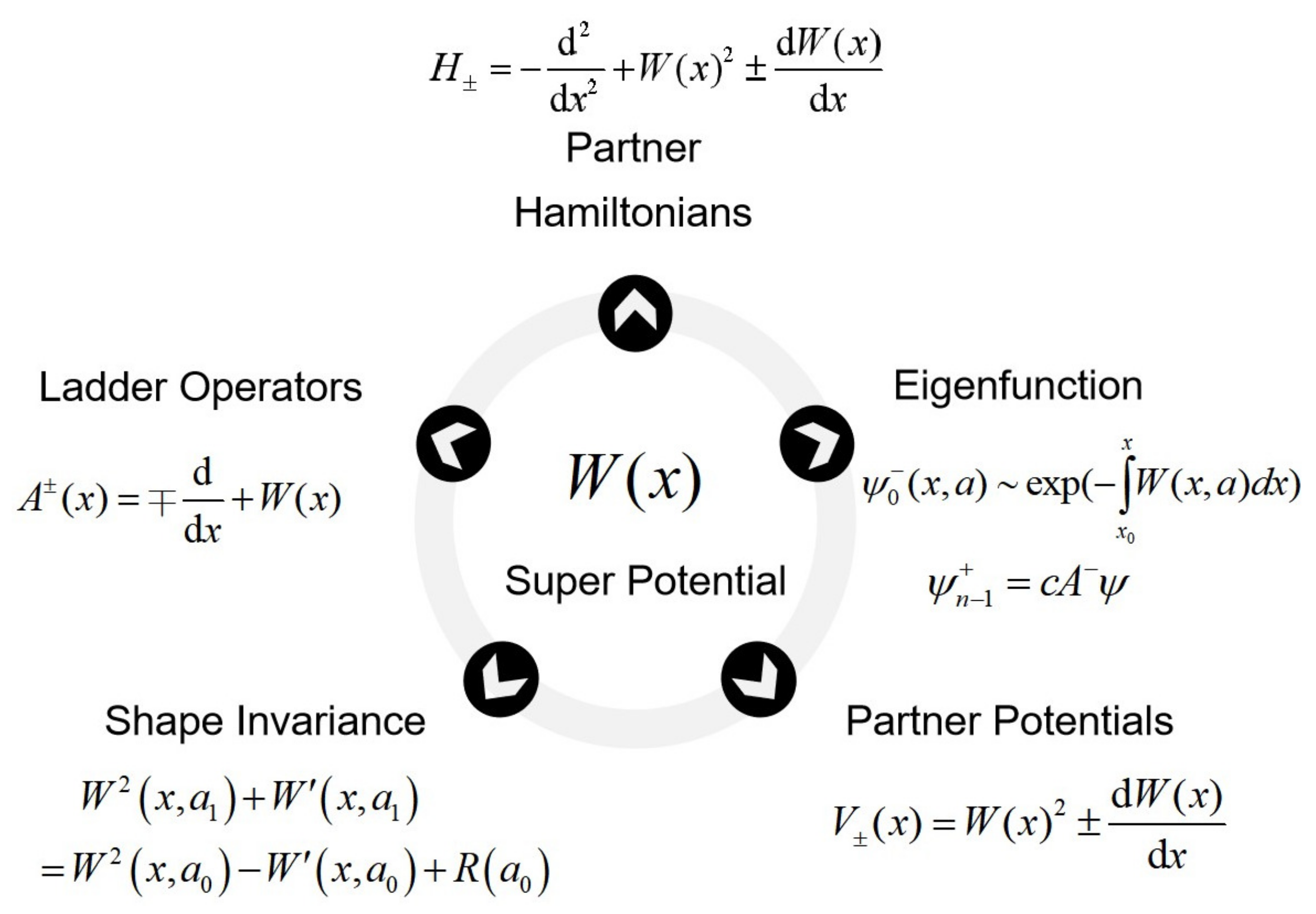
In SUSYQM, as long as a superpotential $W\left(x\right)$ that can be solved accurately is determined, the corresponding ascending and descending operators $A^{\pm }(x,a)$, partner potentials $V_{\pm }(x,a)$, and partner Hamiltonians $H_{\pm }$ can be constructed according to this superpotential $W\left(x\right)$, so as to solve the corresponding eigen energy $E_n^{-}\left(a_i\right)(i=0,1,2,\dots )$ and eigen wavefunction ${\psi }_n^{-}\left(x\right)$. The relationship between the superpotential and these physical quantities can be described by Figure 1.

Figure 1 shows the importance of superpotential in SUSYQM. But the number of potentials that can be solved exactly at present is very limited.

Table A1. The newly constructed potential that can be solved exactly.

Name	Superpotential	Eigenenergies	Ground State Eigenfunction
Generalized Hyperbolic Tangent 1	$$A\tanh npx+B\tanh mpx$$	$${(A+B)}^2-{(A+B-knp-kmp)}^2$$	$${\left(\cosh npx\right)}^{-\frac{A}{np}}{\left(\cosh mpx\right)}^{-\frac{B}{mp}}$$
Generalized Hyperbolic Tangent 2	$$A\tanh px+B\tanh 6px$$	$${(A+B)}^2-{(A+B-7np)}^2$$	$$\cosh p{x}^{\frac{1}{2}\left(-1+\frac{B_0}{6p}\right)}\cosh 6p{x}^{-\frac{B_0}{6p}}$$
Generalized Hyperbolic Tangent 3	$$\left(-\frac{b}{2}+p\right)\tanh px+b\tanh 2px$$	$${\left(\frac{1}{2}b+p\right)}^2-{\left(\frac{1}{2}b-(n+1)p\right)}^2$$	$$\cosh p{x}^{-1+\frac{b_0}{2p}}\cosh 2p{x}^{-\frac{b_0}{2p}}$$
Generalized Hyperbolic Tangent 4	$$\frac{1}{4}(-b+4p)\tanh px+b\tanh 4px$$	$${\left(\frac{3}{4}b+p\right)}^2-{\left(\frac{3}{4}b-(3n+1)p\right)}^2$$	$$\cosh p{x}^{\frac{b}{4p}}\cosh 4p{x}^{1-\frac{b}{4p}}$$
Generalized trigonometric tangent (this paper)	$$\Lambda \tan npx+B\tan mpx$$	$$\begin{array}{cc}\hfill & {\left(A_0+nkp\right)}^2+\left(B_0\right.\hfill \\ \hfill & {+mkp)}^2-A_0^2-B_0^2\hfill \end{array}$$ (A1)	$$N_0{\left(\cos mpx\right)}^{\frac{B_0}{mp}}{\left(\cos mpx\right)}^{\frac{A_0}{np}}$$

and

Table A2. Exactly solvable potentials constructed long ago.

Name	Superpotential	Eigenenergies	Ground State Eigenfunction
Harmonic oscillator	$\frac{1}{2}\omega x$	$n\omega$	$\exp \left(-\frac{1}{4}\omega x^2\right)$
3-D Oscillator	$\frac{1}{2}\omega r-\frac{\ell +1}{r}$	$2n\omega$	$r^{l+1}\exp \left(-\frac{\omega r^2}{4}\right)$
Coulomb	$$\frac{e^2}{2(\ell +1)}-\frac{\ell +1}{r}$$	$$\frac{1}{4}\left[{\left(\frac{e^2}{\ell +1}\right)}^2-{\left(\frac{e^2}{\ell +n+1}\right)}^2\right]$$	$$r^{\ell +1}\exp \left(-\frac{1}{2}\frac{e^2}{\ell +1}r\right)$$
Morse	$$A-e^{-x}$$	$$A^2-{(A-n)}^2$$	$$\exp \left[-\left(Ax+\frac{B}{\alpha }{e}^{-\alpha x}\right)\right]$$
Scarf (hyperbolic)	$$A\tanh x+B\mathrm{sech}x$$	$$A^2-{(A-n)}^2$$	$${\left(\mathrm{sech}\alpha x\right)}^{A/\alpha }\exp \left[-2B{\tan }^{-1}\left(e^{\alpha x}\right)\right]$$
Scarf (trigonometric)	$$A\tan x-B\sec x(A>B)$$	$${(A+n)}^2-A^2$$	$${\left(\cos \frac{x}{2}-\sin \frac{x}{2}\right)}^{A-B}{\left(\sin \frac{x}{2}+\cos \frac{x}{2}\right)}^{A+B}$$
Rosen–Morse (trigonometric)	$$-A\cot x-\frac{B}{A}$$	$$\begin{array}{cc}& {(A+n)}^2-A^2+B^2\left[\frac{1}{A^2}\right.\left.-\frac{1}{{(A+n)}^2}\right]\hfill \end{array}$$	$$\exp \left(\frac{Bx}{A}\right){\sin }^{A}x$$
Rosen–Morse (hyperbolic)	$$A\tanh \alpha x+\frac{B}{A}\left(B<A^2\right)$$	$$\begin{array}{cc}& A^2-{(A-n)}^2-\frac{B^2}{{(A-n)}^2}+\frac{B^2}{A^2}\hfill \end{array}$$	$${\left(\mathrm{sech}\alpha x\right)}^{A/\alpha }\exp \left(-\frac{Bx}{A}\right)$$
Eckart (hyperbolic)	$$-A\coth r+\frac{B}{A}\left(B>A^2\right)$$	$$\begin{array}{ccc}& A^2-{(A+n)}^2\hfill & \hfill +B^2\left[\frac{1}{A^2}-\frac{1}{{(A+n)}^2}\right]\end{array}$$	$${\left(\sinh \alpha r\right)}^{A/\alpha }\exp \left(-\frac{Br}{A}\right)$$
Eckart (trigonometric)	$$-A\cot \alpha x+B\csc \alpha x(A>B)$$	$${(A+n\alpha )}^2-A^2$$	$$\begin{array}{ccc}& {\left(\sin \alpha x\right)}^{(A-B)/\alpha }\hfill & \hfill {(1+\cos \alpha x)}^{B/\alpha }\end{array}$$
Posch–Teller (hyperbolic)	$$A\coth r-B\mathrm{csch}r$$ $$A<B$$	$$A^2-{(A-n)}^2$$	$$\frac{{\left(\sinh \alpha r\right)}^{(A/\alpha )(B-A)}}{{\left(1+\cosh \alpha r\right)}^{B/\alpha }}$$
Posch–Teller I (hyperbolic)	$$A\tan \alpha x-B\cot \alpha x$$	$${(A+B+2n\alpha )}^2-{(A+B)}^2$$	$${\left(\sin \alpha x\right)}^{B/\alpha }{\left(\cos \alpha x\right)}^{A/\alpha }$$
Posch–Teller II (hyperbolic)	$$A\tan \mathrm{h}r-B\cot \mathrm{h}r(B<A)$$	$${(A-B)}^2-{(A-B-2n\alpha )}^2$$	$$\frac{{\left(\sinh \alpha r^{\circ }\right)}^{B/\alpha }}{{\left(\cosh \alpha r^{*}\right)}^{A/\alpha }}$$

in Appendix A gives all the superpotentials that can be solved exactly at present and the corresponding physical quantities [3,14,15,16,17,18,19,20,21,22,23,24,25,26]. So, whether new superpotentials that can be solved precisely can be constructed has become the focus of research in SUSYQM. Based on this situation, this paper constructs a new superpotential, $A\tan npx+B\tan mpx$, that can be solved exactly.

3. The New Shape Invariance Derivation Idea Based on the New Solvable Potential $\mathbf{A}\mathbf{tan}\mathit{npx}+\mathbf{B}\mathbf{tan}\mathit{mpx}$

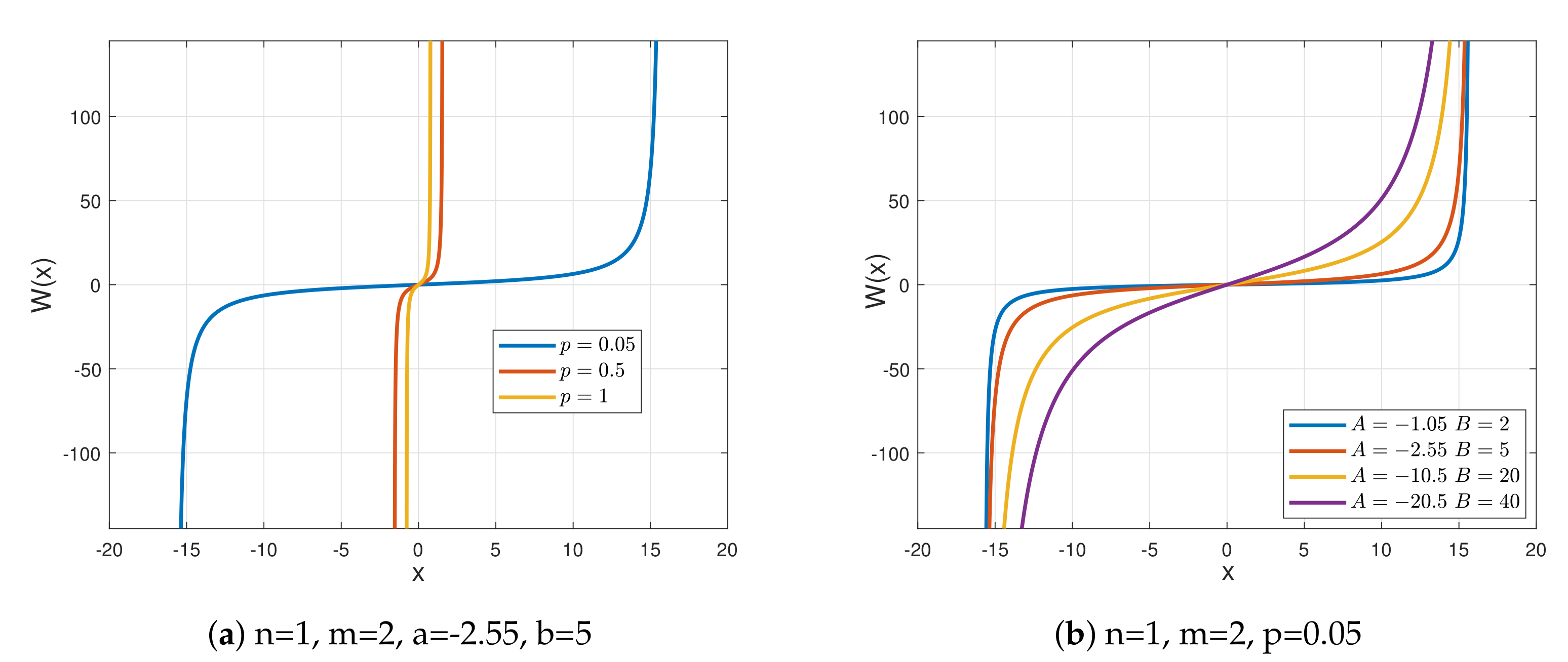
The generalized trigonometric tangent superpotential which we construct is given in Equation (1). The relationship between the superpotential and these parameters are shown in Figure 2.

We can deduce:

$$\begin{array}{cc}\hfill V_{+}(x,A,B)& =W^2(x,A,B)+\frac{\mathrm{d}W(x,A,B)}{\mathrm{d}x}\hfill \\ \hfill =& A(np+A){\sec }^{2}npx+B(mp+B){\sec }^{2}mpx+2AB\tan npx\tan mpx-A^2-B^2\hfill \end{array}$$

(16)

$$\begin{array}{cc}\hfill V_{-}(x,A,B)& =W{(x,A,B)}^2-\frac{\mathrm{d}W(x,A,B)}{\mathrm{d}x}\hfill \\ \hfill =& A(A-np){\sec }^{2}px+B(B-mp){\sec }^{2}mpx+2AB\tan npx\tan mpx-A^2-B^2\hfill \end{array}$$

(17)

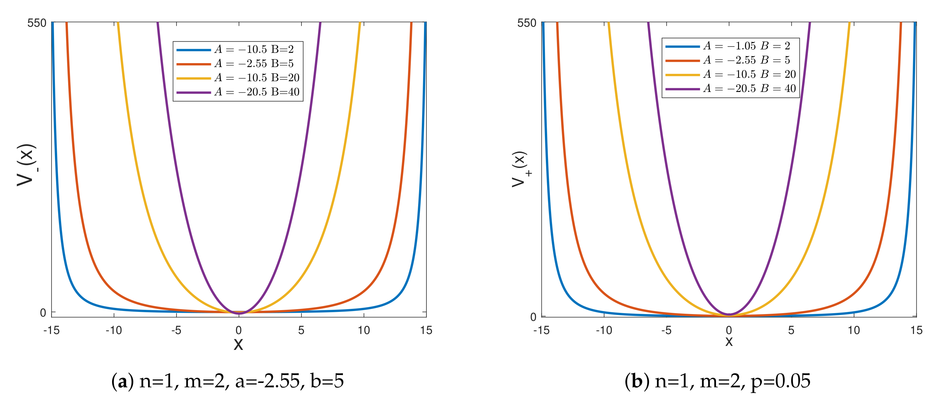
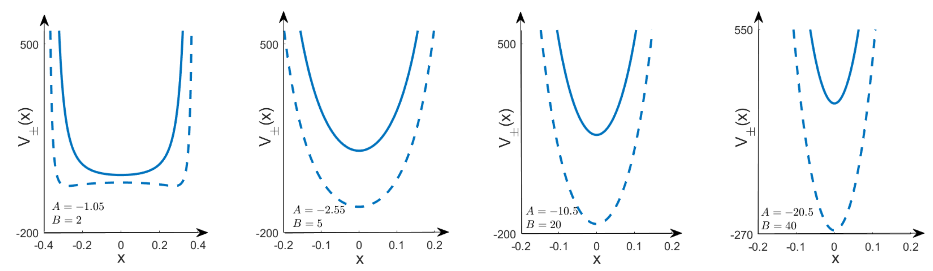
The figures of the partner potentials are shown in Figure 3 and Figure 4. Figure 4 reveals the partner potentials near the origin.

From Figure 3, it can be seen that, whatever values A and B take, the shapes of the partner potentials $V_{-}(x,A,B)$ and $V_{+}(x,A,B)$ are similar, so they conform to the shape invariance relationship described in Section 1.

Now, let us discuss the constraint relationship between $A_0$,$A_1$,$B_0$, and $B_1$. Under the condition of the shape invariance relation of $V_{\pm }(x,A,B)$, the independent variable $\mathrm{x}$ coefficient in $V_{\pm }(x,A,B)$ must be the same, i.e., there are:

$$A_0\left(np+A_0\right)=A_1\left(A_1-np\right)$$

(18)

$$B_0\left(mp+B_0\right)=\left(B_1-mp\right)B_1$$

(19)

$$2A_0{B}_0=2A_1{B}_1$$

(20)

Combining Equations (18)–(20), we can obtain:

$$A_1=A_0+np\mathrm{or}{A}_1=-A_0$$

(21)

$$B_1=B_0+mp\mathrm{or}{B}_1=-B_0$$

(22)

It is not difficult to see that $A_0,A_1,B_0$ and $B_1$ can be combined into the following four cases which are shown in

Table 1. The four cases of $A_1,B_1$.

Case 1	Case 2	Case 3	Case 4
$A_1=A_0+np$	$A_1=A_0+np$	$A_1=-A_0$	$A_1=-A_0$
$B_1=B_0+mp$	$B_1=-B_0$	$B_1=B_0+mp$	$B_1=-B_0$

.

As for case 4, since it does not satisfy the additivity, we do not discuss the case here. Let us analyze the wave function and energy under the other three cases in the following.

3.1. Case 1 $A_1=A_0+np,B_1=B_0+mp$

By substituting $A_1=A_0+np$ and $B_1=B_0+mp$ into Equations (16) and (17), we can obtain:

$$\begin{array}{cc}\hfill V_{+}\left(x,A_0,B_0\right)=& \left(np{A}_0-A_0^2\right){\sec }^{2}npx+\left(mp{B}_0-B_0{}^2\right){\sec }^{2}mpx+\hfill \\ \hfill & 2A_0{B}_0\tan npx\tan mpx-A_0^2-B_0^2\hfill \end{array}$$

(23)

$$\begin{array}{c}{V}_{-}\left(x,A_1,B_1\right)=\left(np{A}_0-A_0^2\right){\sec }^{2}npx+\left(mp{B}_0-B_0^2\right){\sec }^{2}mpx+2\left(A_0+np\right)\\ \left(B_0+mp\right)\tan npx\tan mpx-{\left(A_0+np\right)}^2-{\left(B_0+mp\right)}^2\end{array}$$

(24)

Since the shape invariance relationship is satisfied between $V_{+}\left(x,A_0,B_0\right)$ and $V_{-}\left(x,A_1,B_1\right)$, the coefficients before independent variable x should be equal. That is to say, there is:

$$2A_0{B}_0=2\left(A_0+np\right)\left(B_0+mp\right)$$

(25)

From this formula, the binding relationship between the parameters can be further obtained as:

$$\frac{A_0}{n}=-p-\frac{B_0}{m}$$

(26)

Under this parameter constraint, the shape invariance relation can be written as:

$$V_{+}\left(x,A_0,B_0\right)=V_{-}\left(x,A_1,B_1\right)+{\left(A_0+np\right)}^2+{\left(B_0+mp\right)}^2-\left(A_0^2+B_0^2\right)$$

(27)

It is not difficult to see the expression of $g\left(A_1,B_1\right),g\left(A_0,B_0\right)$ from the above formula that is:

$$g\left(A_1,B_1\right)={\left(A_0+np\right)}^2+{\left(B_0+mp\right)}^2$$

(28)

$$g\left(A_0,B_0\right)=A_0^2+B_0^2$$

(29)

The coefficients $A_k$ and $B_k$ follow an additive relation and are easy to be obtained:

$$A_k=A_0+knp\mathrm{and}{B}_k=B_0+kmp$$

(30)

where $k=0,1,2,\cdots$. The energy eigenvalue can be obtained as:

$$\begin{array}{c}{E}_k^{-}\left(a_i\right)=g\left(a_{k+i}\right)-g\left(a_i\right)\\ ={\left(A_0+(k+i)np\right)}^2+{\left(B_0+(k+i)mp\right)}^2-\left({\left(A_0+inp\right)}^2+{\left(B_0+imp\right)}^2\right)\end{array}$$

(31)

note that $i=0,1,2,\cdots$. When $i=0$, there are:

$$E_k^{(-)}\left(a_0\right)=g\left(a_k\right)-g\left(a_0\right)={\left(A_0+nkp\right)}^2+{\left(B_0+mkp\right)}^2-A_0^2-B_0^2$$

(32)

However, it is worth noting the condition that the shape invariance holds is that the ground state energy is zero, i.e., $E_0^{-}=0$. According to Equation (31), there is:

$$E_0^{+}=E_1={\left(A_0+np\right)}^2+{\left(B_0+mp\right)}^2-A_0^2-B_0^2$$

(33)

For all $k\ge 1$, we have $E_k^{-}\ge 0$ in Equation (31). Through $\frac{A_0}{\eta }+\frac{B_0}{m}=-p$, we can obtain:

$$k\ge -\frac{2(An+Bm)}{p\left(n^2+m^2\right)}$$

(34)

This means that the energy levels have lower limits. For example, if $A=0.195$, $B=-0.49$, $n=1,m=2,p=0.05$, then $k\ge 10$.

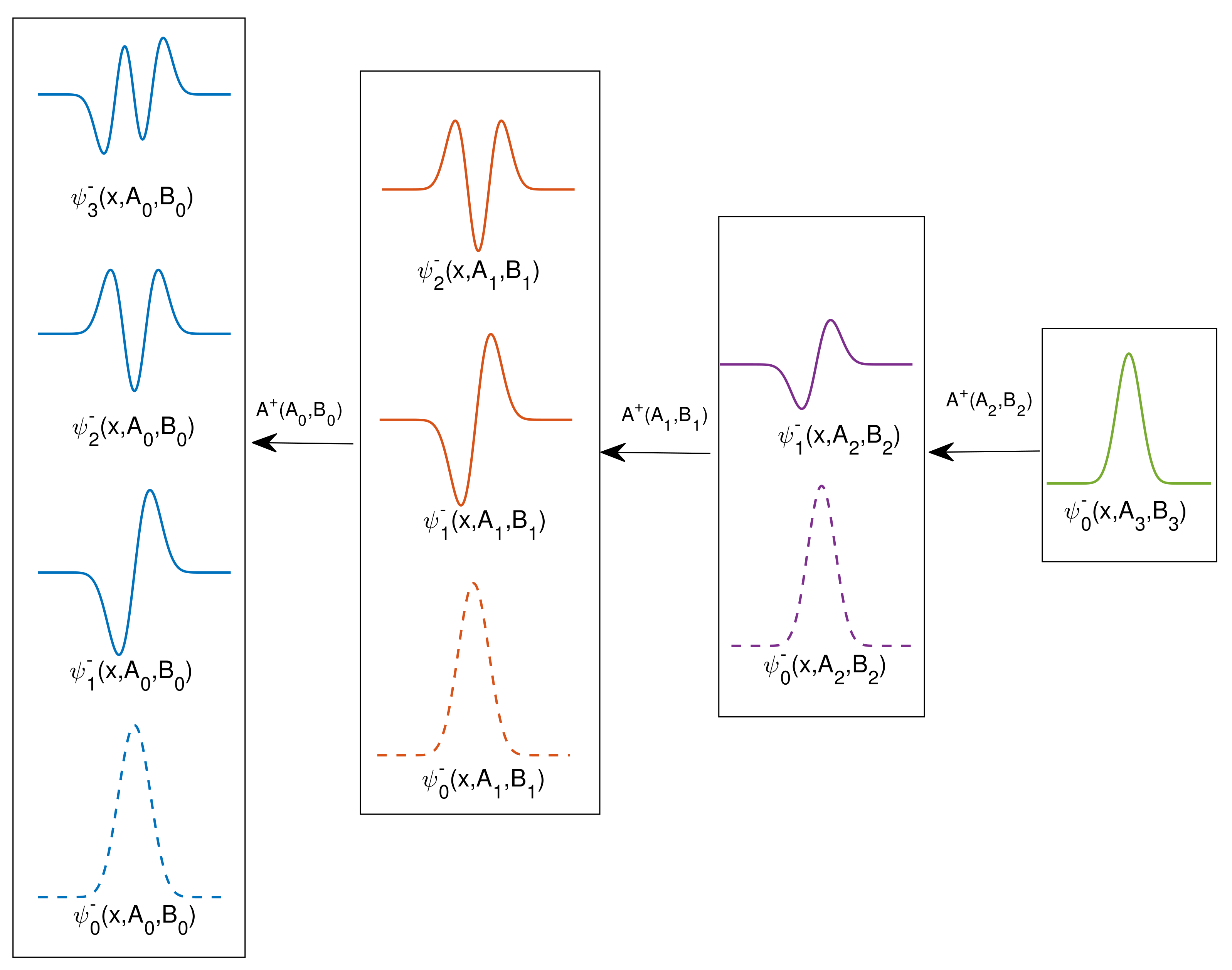
We can also find out the eigenfunctions of the Schrödinger equation:

$${\psi }_k^{-}\left(x,A_0,B_0\right)=N_k{A}^{+}\left(x,A_0,B_0\right)A^{+}\left(x,A_1,B_1\right)\dots A^{+}\left(x,A_{k-1},B_{k-1}\right)e^{-{\int }^{\left(x\right)}W\left(x,A_k,B_k\right)dx}$$

(35)

For example, the ground state wavefunction is:

$${\psi }_0^{(-)}\left(x,A_0,B_0\right)=N_0{e}^{-{\int }^{\left(x\right)}W\left(x,A_0,B_0\right)dx}=N_0{\left(\cos mpx\right)}^{\frac{B_0}{np}}{\left(\cos npx\right)}^{\frac{A_0}{np}}$$

(36)

and the first excited state wavefunction is:

$$\begin{array}{c}{\psi }_1^{-}\left(x,A_0,B_0\right)=N_1{\widehat{A}}^{+}\left(x,A_0,B_0\right)e^{-\int W\left(x,A_1,B_1\right)}\\ =-N_1{\left(\cos npx\right)}^{\frac{A_1}{np}-1}{\left(\cos mpx\right)}^{\frac{B_1}{mp}-1}(np\sin npx\cos mpx+mp\cos npx\sin mpx)\end{array}$$

(37)

where $N_k,N_0$, and $N_1$ are the normalization coefficients. Some of the eigenfunctions and their relationships are shown in Figure 5.

Of course, we can also obtain the eigenwave functions of the other excited states to obtain the exact solutions of the Schrödinger equation.

3.2. Case 2 $A_1=A_0+np,B_1=-B_0$

Putting $A_1=A_0+np$ and $B_1=-B_0$ into Equations (16) and (17), we have:

$$\begin{array}{c}{V}_{+}\left(x,A_0,B_0\right)=A_0\left(np+A_0\right){\sec }^{2}npx+B_0\left(mp+B_0\right){\sec }^{2}mpx\\ +2A_0{B}_0\tan npx\tan mpx-A_0^2-B_0^2\end{array}$$

(38)

$$\begin{array}{c}{V}_{-}\left(x,A_1,B_1\right)=\left(A_0+np\right)A_0{\sec }^{2}npx+B_0\left(B_0+mp\right){\sec }^{2}mpx\\ -2\left(A_0+np\right)B_0\tan npx\tan mpx-{\left(A_0+np\right)}^2-B_0^2\end{array}$$

(39)

Analogously, the coefficients before independent variable x should be equal, that is to say:

$$2A_0{B}_0=-2\left(A_0+np\right)B_0$$

(40)

We can obtain the binding relation between the parameters corresponding to this case, which is:

$$A_0=-\frac{np}{2}$$

(41)

Furthermore, the shape invariance between $V_{+}\left(x,A_0,B_0\right)$ and $V_{-}\left(x,A_1,B_1\right)$ is given by:

$$V_{+}\left(x,A_0,B_0\right)=V_{-}\left(x,A_1,B_1\right)+{\left(A_0+np\right)}^2+B_0^2-A_0^2-B_0^2$$

(42)

In the same way, combining with Equation (5), we can obtain:

$$\begin{array}{cc}\hfill & g\left(A_1,B_1\right)={\left(A_0+np\right)}^2-B_0{}^2\hfill \\ \hfill & g\left(A_0,B_0\right)=A_0^2-B_0{}^2\hfill \end{array}$$

(43)

Since $A_0=-\frac{np}{2}$, substituting it into the above formula, we have:

$$E_1^{-}\left(A_0,B_0\right)=g\left(A_1,B_1\right)-g\left(A_0,B_0\right)=0$$

(44)

By the recurrence of energy according to the shape invariance,

$$A_k=A_0+knp\mathrm{and}{B}_k={(-1)}^k{B}_0$$

(45)

It still needs to satisfy

$$A_k{B}_k=A_{k+1}{B}_{k+1}\Rightarrow A_k{B}_k=\left(A_k+np\right)B_{k+1}$$

(46)

Considering the Equations (41) and (45), we can obtain:

$$A_k=-np/2=A_0$$

(47)

Obviously, it can be seen that the above formula can only exist when $k=0$; otherwise, the energy will be less than 0, which is not allowed. That is to say, only $A_0=-np/2$ and $A_1=np/2$ meet the requirements.

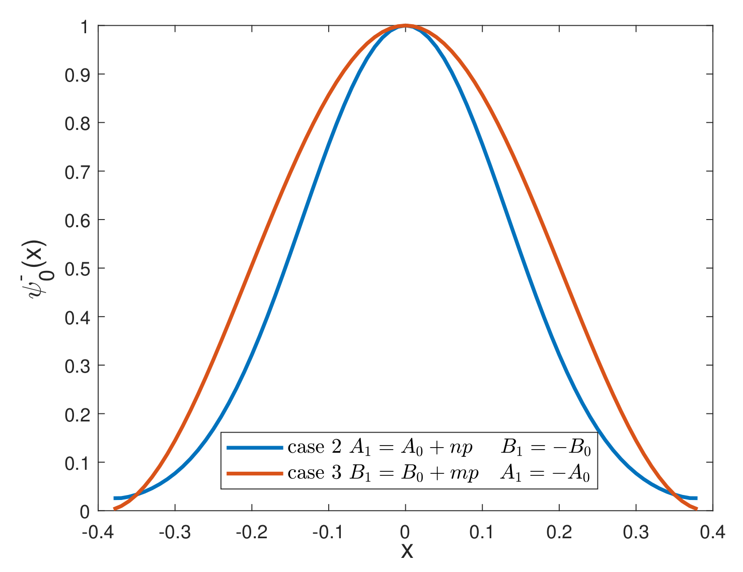
According to Equation (35), we can see that there is only a zero-energy ground state ${\psi }_0^{-}\left(x\right)$:

$${\psi }_0^{(-)}\left(x\right)=N{\left(\cos mpx\right)}^{\frac{B_0}{mp}}{\left(\cos npx\right)}^{-\frac{1}{2}}$$

(48)

where N is the normalization constant. The figure of the ground state ${\psi }_0^{-}\left(x\right)$ is shown in Figure 6.

3.3. Case 3 $B_1=B_0+mp,A_1=-A_0$

This case is similar to the previous one. So, we have $B_0=-mp/2,\left(A_0\ne 0\right)$, and only $B_0=-mp/2$ and $B_1=mp/2$ meet the requirements. Since the ground state energy is zero, we can obtain:

$$E_1^{-}=g\left(A_1,B_1\right)-g\left(A_0,B_0\right)=0$$

(49)

According to Equation (35), there is only a zero energy ground state ${\psi }_0^{-}\left(x\right)$:

$${\psi }_0^{-}\left(x\right)=N^{\prime }{\left(\cos mpx\right)}^{-\frac{1}{2}}{\left(\cos npx\right)}^{\frac{A_0}{np}}$$

(50)

where $N^{\prime }$ is the normalization constant. The figure of the ground state ${\psi }_0^{-}\left(x\right)$ is shown in Figure 6.

From the research in the Section 3, it can be seen that the new potential $A\tan npx+B\tan mpx$ constructed in this paper can not only be precisely solved by SUSYQM but also has some special features compared with the previous potential (Appendix A); for example, it has a variety of shape invariance relationships and more rigid parameter binding relationships, which are shown in Table 2.

Table 2. The physical quantities of the new Superpotential $W(x,A,B)=A\tan npx+B\tan mpx$.

	Variation of Parms	Binding of Parms	Value of k	Eigen Energy ${\mathit{E}}_{\mathit{k}}^{(-)}$	Ground State ${\mathit{\psi }}_0^{-}\left(\mathit{x}\right)$
Case 1	$$\begin{array}{c}{A}_k=A_0+knp\\ B_k=B_0+kmp\end{array}$$ (51)	$\frac{A_0}{n}=-p-\frac{B_0}{m}$	$0,1,2\dots$	$$\begin{array}{cc}\hfill & {\left(A_0+nkp\right)}^2+\left(B_0\right.\hfill \\ \hfill & {+mkp)}^2-A_0^2-B_0^2\hfill \end{array}$$ (52)	$N_0{\left(\cos mpx\right)}^{\frac{B_0}{mp}}{\left(\cos mpx\right)}^{\frac{A_0}{np}}$
Case 2	$$\begin{array}{c}{A}_k=A_0+knp\\ B_k={(-1)}^k{B}_0\end{array}$$ (53)	$A_0=-\frac{np}{2}$	0	0	$N{\left(\cos mpx\right)}^{\frac{B_0}{mp}}{\left(\cos npx\right)}^{-\frac{1}{2}}$
Case 3	$$\begin{array}{cc}\hfill & A_k={(-1)}^n{A}_0\hfill \\ \hfill & B_k=B_0+kmp\hfill \end{array}$$ (54)	$B_0=-\frac{mp}{2}$	0	0	$N^{\prime }{\left(\cos mpx\right)}^{-\frac{1}{2}}{\left(\cos npx\right)}^{\frac{A_0}{np}}$

Table 2. The physical quantities of the new Superpotential $W(x,A,B)=A\tan npx+B\tan mpx$.

	Variation of Parms	Binding of Parms	Value of k	Eigen Energy ${\mathit{E}}_{\mathit{k}}^{(-)}$	Ground State ${\mathit{\psi }}_0^{-}\left(\mathit{x}\right)$
Case 1	$$\begin{array}{c}{A}_k=A_0+knp\\ B_k=B_0+kmp\end{array}$$ (51)	$\frac{A_0}{n}=-p-\frac{B_0}{m}$	$0,1,2\dots$	$$\begin{array}{cc}\hfill & {\left(A_0+nkp\right)}^2+\left(B_0\right.\hfill \\ \hfill & {+mkp)}^2-A_0^2-B_0^2\hfill \end{array}$$ (52)	$N_0{\left(\cos mpx\right)}^{\frac{B_0}{mp}}{\left(\cos mpx\right)}^{\frac{A_0}{np}}$
Case 2	$$\begin{array}{c}{A}_k=A_0+knp\\ B_k={(-1)}^k{B}_0\end{array}$$ (53)	$A_0=-\frac{np}{2}$	0	0	$N{\left(\cos mpx\right)}^{\frac{B_0}{mp}}{\left(\cos npx\right)}^{-\frac{1}{2}}$
Case 3	$$\begin{array}{cc}\hfill & A_k={(-1)}^n{A}_0\hfill \\ \hfill & B_k=B_0+kmp\hfill \end{array}$$ (54)	$B_0=-\frac{mp}{2}$	0	0	$N^{\prime }{\left(\cos mpx\right)}^{-\frac{1}{2}}{\left(\cos npx\right)}^{\frac{A_0}{np}}$

4. Potential Algebra of the New Superpotential $\mathbf{A}\mathbf{tan}\mathit{npx}+\mathbf{B}\mathbf{tan}\mathit{mpx}$

The solution and the shape invariances of Equation (5) can also be obtained by potential algebra [29,30,31,32]. Let us introduce the operators $J_3,J_{+}$ and $J_{-}$ [34,35,36,37] ($J_3$ is a Casimir operator):

$$J_{+}=e^{is\varphi }{\mathcal{A}}^{+},J_{-}={\mathcal{A}}^{-}{e}^{-is\varphi },J_3=k-\frac{i}{s}{\partial }_{\varphi },F\left(J_3\right)=f\left(\chi \left(sk-s{J}_3\right)\right)$$

(55)

where s is a constant which reflects the additive step length, and k is an arbitrary constant, the function $\chi$ must satisfy the compatibility equation: $\chi \left(i{\partial }_{\theta }+s\right)=\eta \left(\chi \left(i{\partial }_{\theta }\right)\right)$ in which $\eta \left(\chi \left(i{\partial }_{\theta }\right)\right)$ is a function of function $\chi \left(i{\partial }_{\theta }\right),\varphi$ is an auxiliary variable, the operator ${\mathcal{A}}^{-}$ is obtained from $A^{-}\left(x,a_0\right)$ by introducing an auxiliary variable $\varphi$ independent of $\mathrm{z}$ and replacing the parameter ${\mathrm{a}}_0$ with an operator $\chi \left(i{\partial }_{\theta }\right)$ [34,35]:

$$x\to z,a_0\to \chi \left(i{\partial }_{\varphi }\right),a_1\to \chi \left(i{\partial }_{\varphi }+s\right),A^{-}\left(x,a_0\right)\to {\mathcal{A}}^{-}\left(z,\chi \left(i{\partial }_{\varphi }\right)\right)$$

(56)

and $J_{\pm }$ have the characteristics of raising and lowering operators:

$$\begin{array}{cc}\hfill & \left[J_{+},J_{-}\right]=J_{+}{J}_{-}-J_{-}{J}_{+}\hfill \\ \hfill & ={\mathrm{e}}^{is\varphi }{\mathcal{A}}^{+}\left(z,\chi \left(i{\partial }_{\varphi }\right)\right){\mathcal{A}}^{-}\left(z,\chi \left(i{\partial }_{\varphi }\right)\right){\mathrm{e}}^{-is\varphi }-{\mathcal{A}}^{-}\left(z,\chi \left(i{\partial }_{\varphi }\right)\right){\mathcal{A}}^{+}\left(z,\chi \left(i{\partial }_{\varphi }\right)\right)\hfill \\ \hfill & ={\mathcal{A}}^{+}\left(z,\chi \left(i{\partial }_{\varphi }+s\right)\right){\mathcal{A}}^{-}\left(z,\chi \left(i{\partial }_{\varphi }+s\right)\right)-{\mathcal{A}}^{-}\left(z,\chi \left(i{\partial }_{\varphi }\right)\right){\mathcal{A}}^{+}\left(z,\chi \left(i{\partial }_{\varphi }\right)\right)\hfill \end{array}$$

(57)

In addition, $J_3$ satisfies the following properties:

$$e^{\pm is\phi }{J}_3{e}^{\mp is\phi }=J_3\pm s,e^{\pm is\phi }{J}_3{}^2{e}^{\mp is\phi }={\left(J_3\pm s\right)}^2$$

(58)

For further discussion, see Reference [35]. The commutations of $J_{+},J_{-}$ and $J_3$ are satisfied with:

$$\left[J_3,J_{\pm }\right]=\pm J_{\pm }\left[J_{+},J_{-}\right]=F\left(J_3\right)$$

(59)

For the general algebra described in Equation (58), these operators are explicitly checked:

$$J_{-}{J}_{+}+G\left(J_3\right)=J_{+}{J}_{-}+G\left(J_3-1\right),F\left(J_3\right)=G\left(J_3\right)-G\left(J_3-1\right)$$

(60)

where $G\left(J_3\right)$ is a function of $J_3$. Suppose $\mid h>$ is an arbitrary eigenstate of $J_3$, and $J_{\pm }$ plays the role of raising and lowering operators. Then, there are:

$$J_3|h>=h|h>,J_{-}|h>=a\left(h\right)|h-1>,J_{+}|h>=a(h+1)|h+1>$$

(61)

where $a\left(h\right)$ is a function of eigenvalue h. According to $\left[J_{+},J_{-}\right]\left|h>=F\left(J_3\right)\right|h>$, we obtain:

$$J_{+}{J}_{-}-J_{-}{J}_{+}={\left|a\left(h\right)\right|}^2-{\left|a(h+1)\right|}^2=G\left(h\right)-G(h-1)$$

(62)

If $h=h_{min}$, then $J_{-}\left|h_{min}\right.〉=0$ and $a\left(h_{min}\right)=0$, we have:

$$a^2\left(h_{min}+1\right)=G\left(h_{min}-1\right)-G\left(h_{min}\right)$$

(63)

By substituting Equation (63) into Equation (62), we have:

$${\left|a\left(h_{min}+2\right)\right|}^2=G\left(h_{min}-1\right)-G\left(h_{min}+1\right)$$

(64)

Repeating the above steps, we can obtain:

$$a^2\left(h_{min}+k\right)=G\left(h_{min}-1\right)-G\left(h_{min}+k-1\right)$$

(65)

where k is a positive integer. If $h_{min}+k=h$, then:

$$a^2\left(h\right)=G(h-k-1)-G(h-1)$$

(66)

From Equations (62) to (66), the expression of $G\left(J_3\right)$ is critical which can be determined by $\mathcal{H}=J_{+}{J}_{-}.$ If $\mathcal{H}$, is allowed to act on the state ${\psi }_n\left(x\right)$, the following relation can be obtained:

$${\mathcal{H}}_{-}{\psi }_n\left(x\right)=J_{+}{J}_{-}{\psi }_n\left(x\right)=E_n^{-}{\psi }_n\left(x\right)=(G(h-k-1)-G(h-1)){\psi }_n\left(x\right)$$

(67)

Next, we need to find the potential algebra presentation ${\mathcal{H}}_{\pm }$ and $\tilde{h}$ of H and h for this new potential $A\tan \left(npx\right)+B\tan \left(mpx\right)$. Since this new solvable potential has two parameters, it is not difficult to imagine that the potential algebra constructed should also have two parameters. According to Equation (9), we can obtain:

$$\begin{array}{c}{\mathcal{H}}_{+}\left(x,{\chi }_A\left(i{\partial }_{\varphi A}\right),{\chi }_B\left(i{\partial }_{\varphi B}\right)\right)={\mathcal{H}}_{-}\left(x,\chi \left(i{\partial }_{\varphi A}+s_A\right),\chi \left(i{\partial }_{\varphi B}+s_B\right)\right)+\\ \tilde{h}\left(\chi \left(i{\partial }_{\varphi A}+s_A\right),\chi \left(i{\partial }_{\varphi B}+s_B\right)\right)-\tilde{h}\left(\chi \left(i{\partial }_{\varphi A}\right),\chi \left(i{\partial }_{\varphi B}\right)\right)\end{array}$$

(68)

with Equations (21) and (22), we have

$$s_A=np,s_B=mp$$

(69)

Let $\chi \left(z\right)=z$, then

$$i{\partial }_{\varphi A}=np\left(k_A-J_3^A\right),i{\partial }_{\varphi B}=mp\left(k_B-J_3^B\right)$$

(70)

Since parameters in need to satisfy the additivity, there are constraints similar to Equations (18)–(20), and there exist three cases:

Case (i): $\chi \left(i{\partial }_{\varphi A}+s_A\right)=np\left(k_A-J_3^A+1\right),B_1=-B_0$ (the parameter A satisfies the additivity);

Case (ii): $A_1=-A_0;\chi \left(i{\partial }_{\varphi B}+s_B\right)=mp\left(k_B-J_3^B+1\right)$ (the parameter B satisfies the additivity);

Case (iii): $\chi \left(i{\partial }_{\varphi A}+s_A\right)=np\left(k_A-J_3^A+1\right),\chi \left(i{\partial }_{\varphi B}+s_B\right)=mp\left(k_B-J_3^B+1\right)$ (both A and B satisfy the additivity).

4.1. Potential Algebra Method with One Parameter

In the above three cases, Case (i) and Case (ii) belong to the single-parameter additive shape invariance, and the discussion of Case (ii) and Case (i) is very similar. So, in this part, we only make careful calculation for Case (i) and directly give the results for Case (ii).

For Case (i), according to Equations (55), (56), and (70), we have:

$$J_3^A=k_A-\frac{i}{s_A}{\partial }_{\varphi A},i{\partial }_{\varphi A}=s_A\left(k_A-J_3^A\right)=np\left(k_A-J_3^A\right),B_1=-B_0$$

(71)

and

$$\begin{array}{c}{J}_{+}{J}_{-}=e^{i{s}_A{\varphi }_A}\left[-\frac{d}{dx}+np\left(k_A-J_3^A\right)\tan npx-B_0\tan mpx\right]\\ \left[\frac{d}{dx}+np\left(k_A-J_3^A\right)\tan npx-B_0\tan mpx\right]e^{-i{s}_A{\varphi }_A}\\ =-\frac{d^2}{d{x}^2}+\left(B_{0}mp+B_0^2\right){\sec }^{2}mpx+n^2{p}^2\left(k_A-J_3^A-np\right)\\ \left(k_A-J_3^A-np-1\right){\sec }^{2}npx-2B_{0}np\left(k_A-J_3^A+np\right)\tan npx\tan mpx\\ -B_0^2-n^2{p}^2{\left(k_A-J_3^A-np\right)}^2\end{array}$$

(72)

$$\begin{array}{cc}\hfill J_{-}{J}_{+}=& \left[\frac{d}{dx}+np\left(k_A-J_3^A\right)\tan npx+B_0\tan mpx\right]\left[-\frac{d}{dx}+np\left(k_A-J_3^A\right)\tan npx+B_0\tan mpx\right]\hfill \\ \hfill =& -\frac{d^2}{d{x}^2}+\left(B_{0}mp+B_0^2\right){\sec }^{2}mpx+n^2{p}^2\left(k_A-J_3^A\right)\left(k_A-J_3^A+1\right){\sec }^{2}npx+\hfill \\ \hfill & \mid 2B_{0}np\left(k_A-J_3^A\right)\tan npx\tan mpx-B_0^2-n^2{p}^2{\left(k_A-J_3^A\right)}^2\hfill \end{array}$$

(73)

Furthermore, we have:

$$J_{+}{J}_{-}-J_{-}{J}_{+}=-n^2{p}^2\left[-2\left(k_A-J_3^A\right)np+n^2{p}^2\right]+2B_0{n}^2{p}^2\tan npx\tan mpx$$

(74)

Due to the additional conditional limitations, the coefficient of the term containing the variable x can be made zero by limiting the value of k. That is, it is required that:

$$2B_0{\left(np\right)}^2=0$$

(75)

$$J_{+}{J}_{-}-J_{-}{J}_{+}=0=F\left(J_3^A\right)$$

(76)

In view of Equation (76), apparently, $G\left(J_3^A\right)=G\left(J_3^A-np\right)$ and $F\left(J_3\right)=0$. It indicates that only a single state exists in the system, and its eigenvalue is zero. This result is the same as the shape invariance counterpart in Section 3.2 and Section 3.3.

4.2. Potential Algebra Method with Two Parameters

According to Equations (55), (59), and (70), we have

$$\begin{array}{cc}\hfill J_{+}{J}_{-}=& {\mathrm{e}}^{i\left(s_A{\varphi }_A+s_B{\varphi }_B\right)}{\mathcal{A}}^{+}\left(z,\chi \left(i{\partial }_{{\varphi }_A},{\partial }_{{\varphi }_B}\right)\right){\mathcal{A}}^{-}\left(z,\chi \left(i{\partial }_{{\varphi }_A},{\partial }_{{\varphi }_B}\right)\right){\mathrm{e}}^{-i\left(s_A{\varphi }_A+s_B{\varphi }_B\right)}\hfill \\ \hfill =& \left.{\mathcal{A}}^{+}\left(z,\chi \left(i{\partial }_{{\varphi }_A}+s_A,i{\partial }_{{\varphi }_B}+s_B\right)\right)\right){\mathcal{A}}^{-}\left(z,\chi \left(i{\partial }_{{\varphi }_A}+s_A,i{\partial }_{{\varphi }_B}+s_B\right)\right)\hfill \\ \hfill =& \left[-\frac{d}{dx}+np\left(k_A-J_3^A+1\right)\tan npx+mp\left(k_B-J_3^B+1\right)\tan mpx\right]\hfill \\ \hfill & \left[\frac{d}{dx}+np\left(k_A-J_3^A+1\right)\tan npx+mp\left(k_B-J_3^B+1\right)\tan mpx\right]\hfill \\ \hfill =& -\frac{d^2}{d{x}^2}+{\left(np\right)}^2\left(k_A-J_3^A+1\right)\left(k_A-J_3^A\right){\sec }^{2}npx+{\left(mp\right)}^2\left(k_B-J_3^B+1\right)\hfill \\ \hfill & \left(k_B-J_3^B\right){\sec }^{2}mpx+2mn{p}^2\tan npx\tan mpx-{\left(np\right)}^2{\left(k_A-J_3^A+1\right)}^2\hfill \\ \hfill & -{\left(mp\right)}^2{\left(k_B-J_3^B+1\right)}^2\hfill \end{array}$$

(77)

$$\begin{array}{cc}\hfill J_{-}{J}_{+}=& {\mathcal{A}}^{-}\left(z,\chi \left(i{\partial }_{{\varphi }_A},i{\partial }_{{\varphi }_B}\right)\right){\mathrm{e}}^{-i\left(s_A{\varphi }_A+s_B{\varphi }_B\right)}{\mathrm{e}}^{i\left(s_A{\varphi }_A+s_B{\varphi }_B\right)}{\mathcal{A}}^{+}\left(z,\chi \left(i{\partial }_{{\varphi }_A},i{\partial }_{{\varphi }_B}\right)\right)\hfill \\ \hfill =& {\mathcal{A}}^{-}\left(z,\chi \left(i{\partial }_{{\varphi }_A},i{\partial }_{{\varphi }_B}\right)\right){\mathcal{A}}^{+}\left(z,\chi \left(i{\partial }_{{\varphi }_A},i{\partial }_{{\varphi }_B}\right)\right)\hfill \\ \hfill =& \left[\frac{d}{dx}+np\left(k_A-J_3^A\right)\tan npx+mp\left(k_B-J_3^B\right)\tan mpx\right]\left[-\frac{d}{dx}+np\left(k_A-J_3^A\right)\right.\hfill \\ \hfill & \left.\tan npx+mp\left(k_B-J_3^B\right)\tan mpx\right]\hfill \\ \hfill =& -\frac{d^2}{d{x}^2}+m^2{p}^2\left(k_B-J_3^B+1\right)\left(k_B-J_3^B\right){\sec }^{2}mpx+n^2{p}^2\left(k_A-J_3^A+1\right)\hfill \\ \hfill & \left(k_A-J_3^A\right){\sec }^{2}npx+2mn{p}^2\left(k_B-J_3^B\right)\left(k_A-J_3^A\right)\tan npx\tan mpx\hfill \\ \hfill & -m^2{p}^2{\left(k_B-J_3^B\right)}^2-n^2{p}^2{\left(k_A-J_3^A\right)}^2\hfill \end{array}$$

(78)

Furthermore, we have:

$$\begin{array}{c}{J}_{+}{J}_{-}-J_{-}{J}_{+}={\left(mp\right)}^2{\left(k_B-J_3^B\right)}^2+{\left(np\right)}^2{\left(k_A-J_3^A\right)}^2-\\ \left[{\left(mp\right)}^2{\left(k_B-\left(J_3^B-1\right)\right)}^2+{\left(np\right)}^2{\left(k_A-\left(J_3^A-1\right)\right)}^2\right]\end{array}$$

(79)

Under the requirement of the shape invariance, Equation (79) must be represented only by $J_3$. So, we need to further rewrite the above formula as:

$$J_{+}{J}_{-}-J_{-}{J}_{+}={\left(np\right)}^2\left(2J_3^A-2k_A-1\right)+{\left(mp\right)}^2\left(2J_3^B-2k_B-1\right)$$

(80)

It is not difficult to see that if we set $k_A=-\frac{1}{2},k_B=-\frac{1}{2}$, we obtain:

$$\left[J_{+},J_{-}\right]=2p^2\left(n^2{J}_3^A+m^2{J}_3^B\right)$$

(81)

Considering the function $F\left(J_3\right)$ in Equation (59)

$$J_{+}{J}_{-}-J_{-}{J}_{+}=F\left(J_3\right)=F\left(J_3^A,J_3^B\right)=G\left(J_3^A,J_3^B\right)-G\left(J_3^A-1,J_3^B-1\right)$$

(82)

we can deduce:

$$G\left(J_3^A,J_3^B\right)={\left(mp\right)}^2{\left(-\frac{1}{2}-J_3^B\right)}^2+{\left(np\right)}^2{\left(-\frac{1}{2}-J_3^A\right)}^2$$

(83)

and have

$$E_k^{-}=G\left(h_A-k-1,h_B-k-1\right)-G\left(h_A-1,h_B-1\right)$$

(84)

Set $-\frac{1}{2}-h_A+1=\frac{A}{np},-\frac{1}{2}-h_B+1=\frac{B}{mp}$ and we have the energy eigenvalues

$$E_k^{(-)}\left(a_0\right)={\left(A_0+nkp\right)}^2+{\left(B_0+mkp\right)}^2-A_0^2-B_0^2$$

(85)

This is exactly the same as Equation (32).

5. Summary and Prospect

In this paper, the Schrödinger equation with a new generalized trigonometric tangent superpotential $A\tan npx+B\tan mpx$ is solved within the framework of SUSYQM. We show that the superpotential is the new superpotential that can be solved exactly, which expands the number of exactly solvable potentials shown in Appendix A. At first, the shape invariant relation of partner potential generated by superpotential are discussed from three aspects, which are all satisfied with the additivity, and the energy spectrum and eigenfunctions are obtained. Then, we again study the three aspects with additive shape invariance from the potential algebra, and we obtain the exact same energy eigenvalues as previously. Of course, the exact solutions of the equation can be derived from the ground state wave function. Finally, the energy eigenvalues are discussed.

In conclusion, this paper studies another generalization of the existing solvable potential. Taking the linear combination of $tanmpx$ superpotential and $tannpx$ superpotential as our generalization potential, the results are still exciting. The two generalizations of our research group, including [26], actually give some important information: There are two parameters, and the relationship between the parameters is reversed by the shape invariance, with constraints between the two parameters that meet the shape invariant requirement. These are quite meaningful.