Development of an Interactive Code for Quick Data Analyses between STOR-M Tokamak Experimental Plasma Discharges

Abstract

Saskatchewan Torus-Modified (STOR-M) is a small tokamak, well known for various fusion-related basic experimental studies such as edge turbulent heating, different instabilities, Alternating Current (AC) tokamak operation, Ohmic H-mode triggering by the electrode biasing, fueling and momentum injection by Compact Torus (CT) injection, and the effects of Resonance Magnetic Perturbations (RMPs), among others. Some of those experiments require real-time visualization of magnetic surface reconstructions either through EFIT or quick analyses and visualization of experimental data during experiments. Recently, experimental studies of Geodesic Acoustic Mode (GAM) and zonal flows were performed in the STOR-M tokamak. The GAM experiments strongly require the collection of fluctuation data from different Langmuir probes installed at different poloidal locations, but on the same magnetic surfaces. This is requires the adjustment of radial locations between discharges. It is therefore important to analyze and visualize the features of all probe data quickly during discharges. For this purpose, a Python code was developed and used for quick analysis of the data. This article describes the development of the code using Python and its use in detail.

1. Introduction

The discovery of the concept of zonal flows has great scientific value in the field of basic turbulent plasma physics and magnetically confined plasma systems aiming at nuclear fusion in a controlled manner. A basic requirement to achieve self-sustaining burning plasmas in a magnetically confined fusion reactor is to control the anomalous transportation of particles and energy. It is believed that anomalous transport happens due to small-scale drift turbulent fluctuations in a magnetically confined toroidal system such as tokamaks or stellarators. The anomalous transport can be controlled by radially sheared poloidal flow, which is generated by either a radially sheared mean or oscillating electric field. The poloidal mean flow may be generated by external means, but, in general, the oscillating poloidal flows, confined within a small radial width, are a self-organized process, which is known as “zonal flows”. Theoretically and experimentally, it has been shown that the drift wave turbulence is the sole cause of the origination of zonal flows. Two types of zonal flows have been found in a magnetically confined toroidal plasma system, which are (i) near-zero or very-low-frequency Zonal Flows (ZF) and (ii) Geodesic Acoustic Mode (GAM), which has been found only in toroidal geometry. The conventional GAM features are (i) radially localized, (ii) toroidally axisymmetric for potential and density fluctuations $(n=0;m=0)$ and $k_{\varphi }=0$, and (iii) poloidally symmetric potential fluctuations, and so, $(n=0)$, $k_{\theta }=0$ for potential fluctuations, but asymmetric density fluctuation $(m=1)$ and $k_{\theta }=\pi$ for density fluctuations [1,2].

Since GAM originates in a particular radius and is normally confined within a narrow radial width, the experimental detection of GAM demands that diagnostics should collect data from the same magnetic surfaces where the mode is confined. The main issue of the tokamaks that are not facilitated by good feedback systems is the reproducibility of a particular shot at the same magnetic surface with the same characterizations. Similarly, the radial positions of the GAM formation of a particular tokamak plasma discharge may change shot by shot. In that case, the detection of radial locations of GAM should be performed during real-time operations through quick visualization of the experimental data of the density and potential fluctuations regarding whether they have been collected from the same magnetic surface by the help of highly advanced software such as Equilibrium Fit (EFIT) [3]. A high-performance Python code was developed for quick analysis of the data taken by the diagnostic system and deriving the mode structure between consecutive plasma discharges in STOR-M due to the absence of EFIT.

In this article, a detailed description of the code development, preliminary experimental data analysis through the code during STOR-M discharges, and a brief description of mode detection is discussed.

2. Experimental Setup

The STOR-M has circular plasma cross-section with corresponding major and minor radii 46 cm and 12 cm with plasma discharge duration an around 30 ms. The plasma boundary is determined by using an elliptical shaped stainless steel poloidal limiter, installed in a way that its corresponding internal major (13 cm) and minor (12 cm) radii have oriented along horizontally and vertically. Three Langmuir probe systems (top, radial-2, bottom) were inserted through the top, equatorial and bottom ports of the vessel in the same poloidal cross-section. Another fourth Langmuir probe system (radial-1) is placed equatorially with shifting toroidally by 90° in clockwise direction from top view with respect to the other three Langmuir probe systems, located in the same poloidal cross-section. A detailed description of the diagnostics arrangement can be found in the article “GAM detection in STOR-M tokamak” [4]. Now, a necessary and very important requirement is to determine that all Langmuir probes will collect data from the same magnetic field surface for the GAM detection experimental studies. The main purpose of this code development is a quick determination through fast analysis whether those Langmuir probe data have been collected from the same magnetic surface. The detailed descriptions of the code development is given in the following sections.

3. Code Development

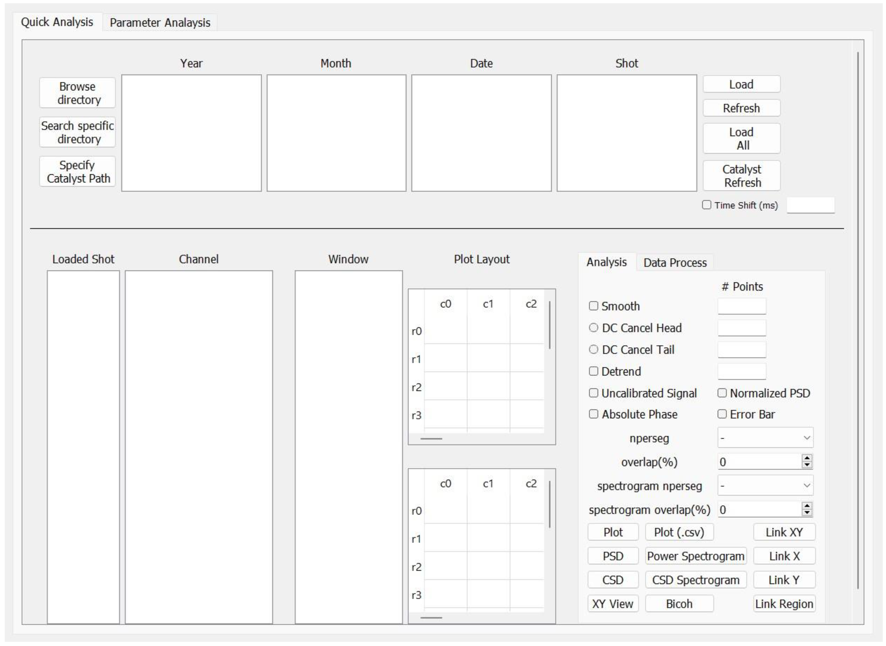
This code uses the Graphical User Interface (GUI) feature in the Python language, specifically for the STOR-M tokamak experiments where the probe data are recorded and stored in National Instruments (NI) digital modules plugged into a “PXI” crate and directly into the PSI slots in the computers. There are around 120 channels in total. LabView software is used to manage all hardware and to transfer onboard data from the digitizers to the computers and save them in the data files on the hard drives of the computers after each shot. In the experimental settings, the duty cycle time period between two discharges can be set to 4–10 min depending on the particular experiments, whereas the time to transfer and save data is completed within a few seconds. It is imperative to quickly visualize and analyze the experimental data after every recorded STOR-M discharge for complex experiments such as GAM detection to determine whether satisfactory data have been obtained or the configuration of the diagnostics setup needs to be modified. The present development of the code with interactive data analysis tools meets such requirements. In this section, the logical frame of the application is discussed. The resulting GUI window is presented in Figure 1. 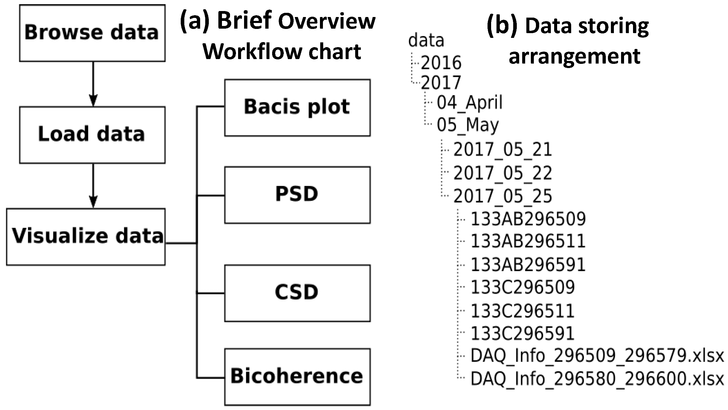The flow of the works of this application is shown in Figure 2a.

It describes how the programs run when the large amount of diagnostics data related to the experiment are stored. periodically after each STOR-M discharge in the pre-specified file in directories. Therefore, each step of the operations and their interconnections from $BrowseData\Rightarrow LoadData\Rightarrow VisualizeData$, the next level of analytical operations, including basic plots, “Power Spectral Density”, “Cross Spectral Density”, and “Bi-coherence”, are controlled by dedicated background programs, which were solely developed for this purpose. Other available applications that were used in a logical manner are the graphical interface through the $\mathtt{PyQt}$ package, a wrapper package for a GUI tool kit $\mathtt{Qt}$ [5], the plotting and visualization of data through $\mathtt{PyQtGraph}$ [6], a python toolkit for interactive data visualization, and the package $\mathtt{SciPy}$ for spectral analysis. Figure 2b represent the sequence of the data arrangement consecutively.

Each STOR-M plasma discharge is labeled by a shot number as a common experimental procedure for data storage. The data files for the National Instrument digitizers are stored in text file format with a unique number synchronized with the shot number corresponding to each set of digitizers within it. It is very important to develop a logical working procedure in the code that includes the methods of reading, interacting, and operating on the stored experimental data. Therefore, this requires a guiding file, which can lead the code in its workflow. Here, an Excel book is the pilot file from which the code collects the instructions for loading the data files. Each Excel pilot file is named in such a way that the code can understand the range of shot numbers stored in a particular folder. The pilot files contain the descriptions for each measurement’s channel names, the conversion factors, and the final unit of the measurement. Since multiple shots share a same measurement setup, the file names of the DAQ information files indicate the range of shot numbers for which the files are applicable. The data files are organized as shown in Figure 2b, showing the pilot excel books and the data files within a folder.

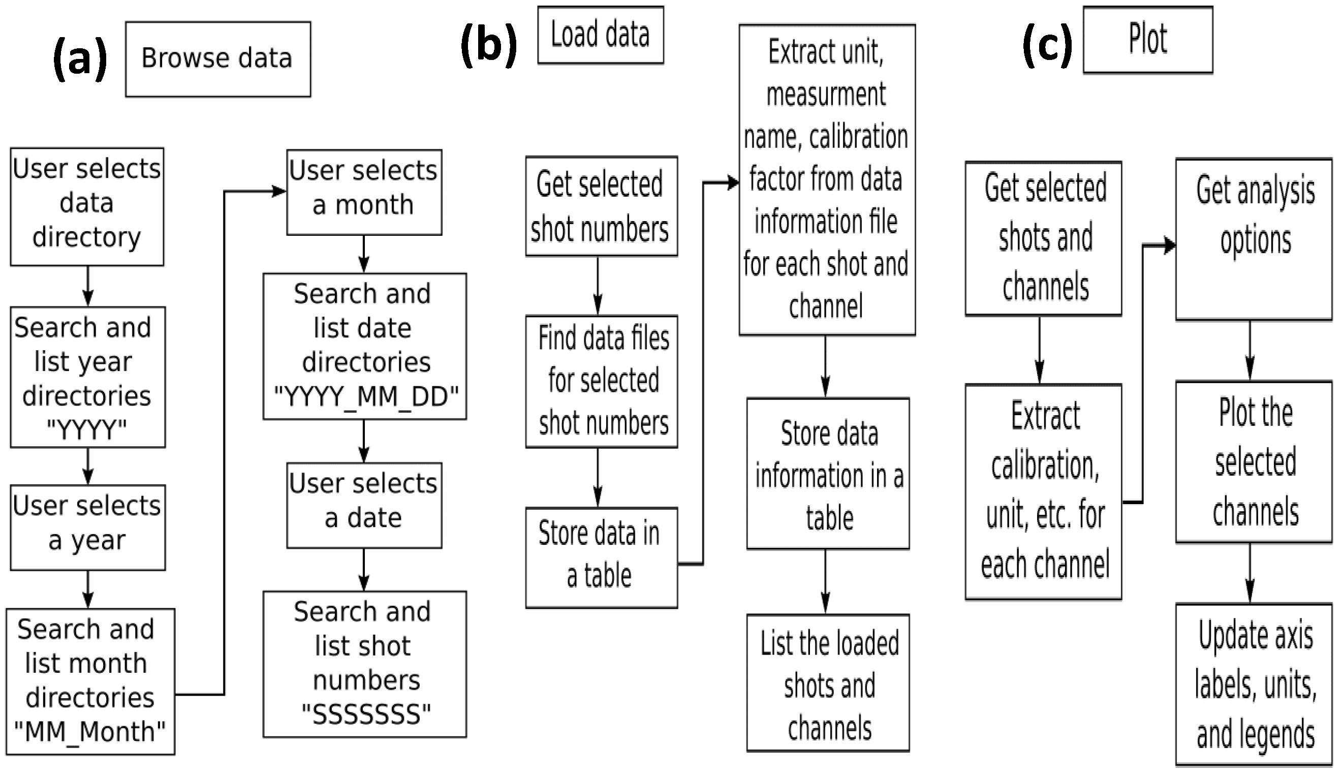
The code starts to load the experimental data in the GUI window shown in Figure 1 through the navigation to the proper directory where the experimental data of interest are stored. This process is performed through the logical flows of “browse data”, shown in Figure 3a. Figure 3b explains the logical flow chart of the “load data” in the GUI window through the interaction with the pilot Excel book, which is one of the key process of the code. Once the shot numbers are available, the shots of interest need to be “loaded” to the program through the GUI window. The program finds all the data files associated with the selected shot numbers. All the files of the selected shot numbers of interest are opened and stored in a table, in particular in the object pandas.DataFrame, which is called the data table, where each of the time series data is given a unique data ID. After that, the program opens the appropriate Excel book and extracts information about the data such as the unit, measurement name, and calibration factor for each data time series. The parameters related to each data ID are stored in another table, which is called the parameter table. The program completes the loading process by listing the shot numbers and measurement names or channels. After proper loading of the data files under analysis, in Figure 3c, the workflow for the basic plots and visualization and the nature of the experimental data are presented.

It is very important to analyze the fundamental signals of various channels to check their proper nature. The program retrieves the information of the relevant data and parameters from the tables of the data and parameters. Optional analyses, such as the smoothing factor, are also possible through the graphical interface. An interactive plot is then generated using a plot item in the pyqtgraph package. Based on these parameters, the program updates the unit, the axis labels, and the legends.

Here, the most important feature of the code is successfully using the in-built ROI tool of pyqtgraph, which allows indicating the Region Of Interest (ROI) and corresponding analysis of the region of the data that is the focus. The ROI can be changed in an interactive fashion, where it can be changed either by modifying the width of the ROI or moving the ROI without changing its width. The corresponding new plot is then updated automatically. This mapping is performed through a function to a signal emitted by the ROI object. In this particular case, the connected function simply plots the data within the selected region. In our application, the ROI tool is a very important feature to carry out spectral analysis, which allows quick and detailed analysis of the modes present in the signals. The ROI tool has been used to efficiently identify GAM within a time series.

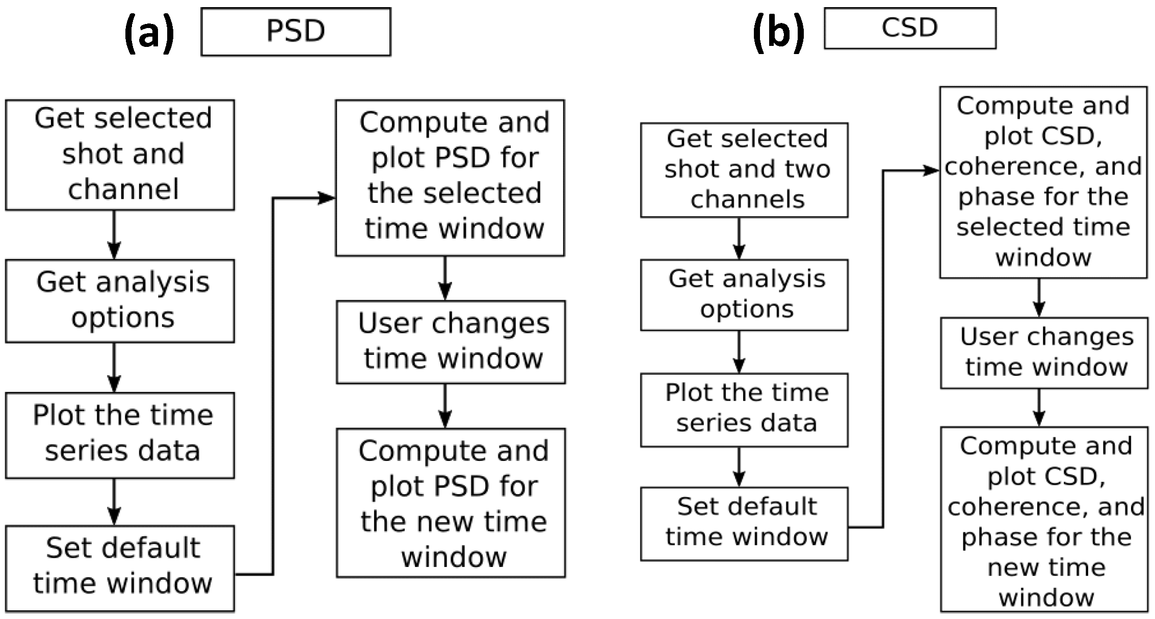
To explain the GAM features, Power Spectral Density (PSD) and cross-power spectral analysis such as Cross-Spectral Density (CSD), cross-coherence, and cross-phase are essential analysis parameters adopted in the code through the GUI from the Python library. Figure 4a,b present the logic flow chart of the PSD and cross-spectral analysis.

The analysis options for the PSD such as segment length and overlap percentage are read from the graphical interface. A default time window is set and visualized as a colored ROI object on the plot of the time series. The PSD is computed using a function in the scipy package and plotted in a separate window within a plot. The time window, an object in the pyqtgraph package, can be changed in an interactive manner. Once the time window is changed, the PSD for the new time range is computed and updated for the corresponding plot.

Cross-spectral analysis is very useful for identifying common modes in two time series signals in the GAM detection experiment. For this process, two time series signals, collected from two different independent channels, are compared. The program also reads the analysis options from the graphical interface such as the “PSD” plot. Initially, the two time series data are plotted. A default time window is set and displayed as a segment item on the time series data, a similar process as for the “PSD” plot. The cross-spectral density, cross-coherence, and cross-phase are computed for the time window and plotted in three separate windows within the plot. When the time window is changed, the above three quantities are computed again for the new time range and the corresponding plots are updated.

4. Results and Discussions

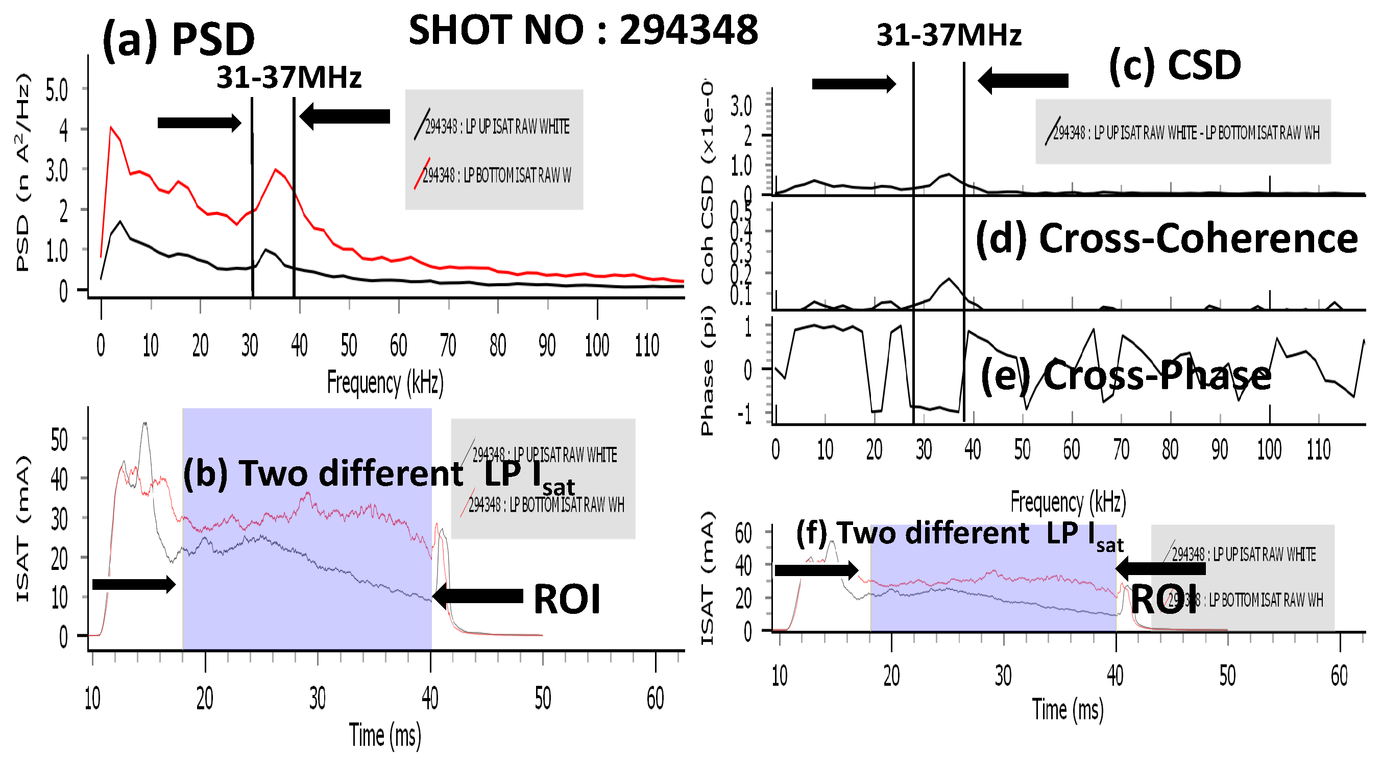
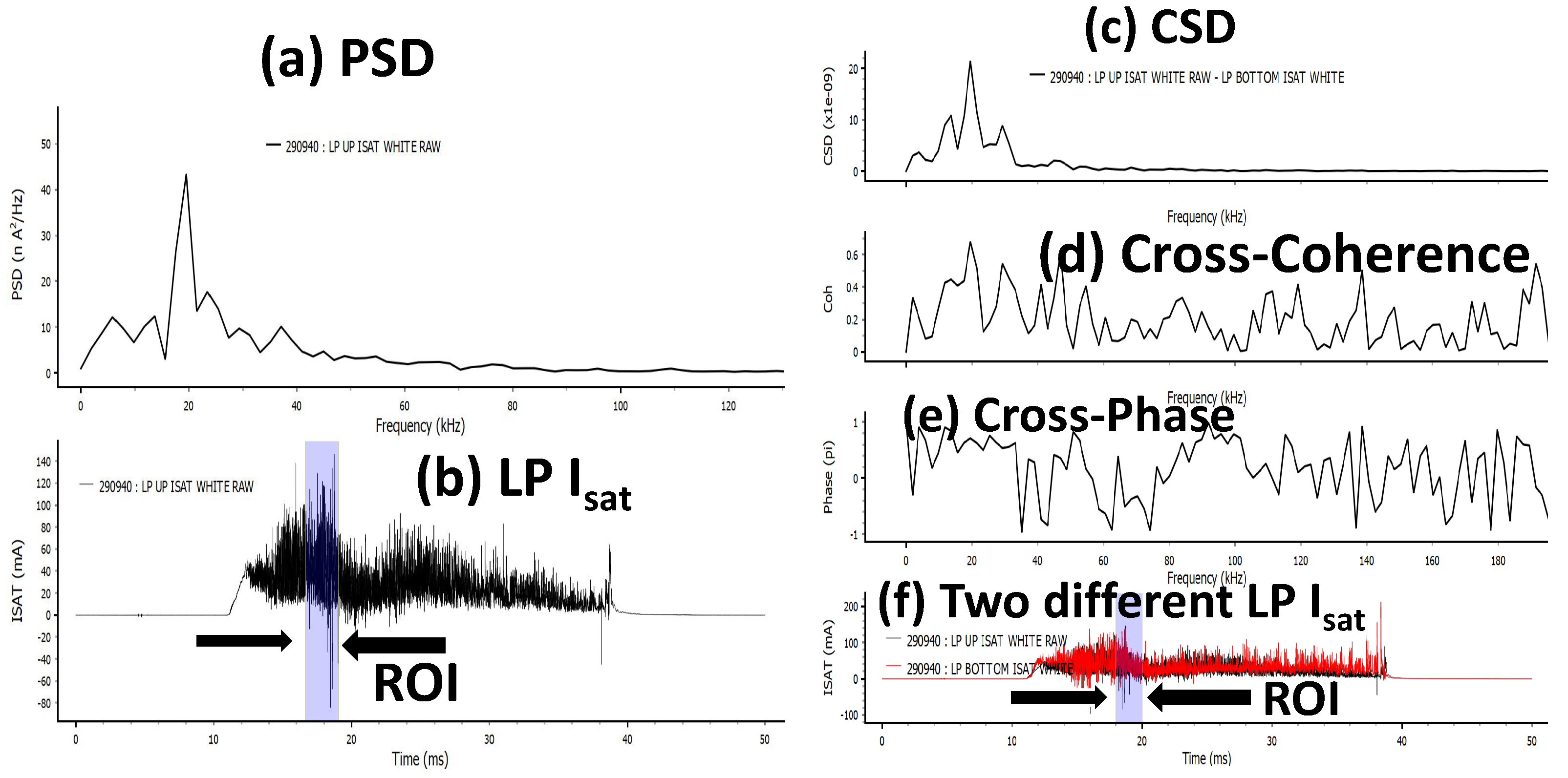
The previous section discussed how the code works. Figure 5 presents a typical example of the basic plots and the corresponding plots of the “PSD”, “CSD”, “Cross-coherence”, and “Cross-phase” at the ROI of the basic data plots. Figure 5a presents the “PSD” of the data regime with the ROI of the basic plot of the ion saturation current of the Langmuir probe, as shown in Figure 5b. Similarly, Figure 5c–e present the “CSD”, “Cross-coherence”, and “Cross-phase” at the ROI data regime of the two different ion saturation current signals collected from two different Langmuir probes. Here, the ROI is marked by the gray rectangular window in the basic plots of Figure 5. Therefore, it is clear from the typical example of Figure 5 that the mode can be easily determined in a time series by changing the ROI positions on the basic data plots, and it is a very powerful tool for GAM detections.

It is well known that the GAM detection experiment is very sophisticated due to its complexity, and it is very important to understand the inherent turbulent physics, as well as the L-H transition in tokamaks or stellarators. It is basically a high-frequency zonal flow [1,2,4,7] and normally confined within a small radial width. Furthermore, recently, it was found that it can be a global eigenmode, as well, which exhibits a long-range spatial correlation [8], but not in all tokamaks or stellarators. Therefore, it is necessary to detect experimentally GAM by collecting the information from approximately the same magnetic field surfaces. The same or nearly the same magnitude of the $I_{sat}$ signal profiles, collected from the top and bottom Langmuir probes during the same plasma discharge, serve as a criterion to indicate that all measured density fluctuations or floating potential fluctuations are accumulated from the same or nearly the same magnetic field surface.

The long-duration or periodically repetitive short-duration modes during whole plasma discharge can be easily derived by the power spectrogram [9,10], where the power spectrum is derived within an optimized time window and repeated in the whole plasma discharge. Initially, a similar analysis was carried out for STOR-M tokamak discharge for GAM detection. However, the appearance of GAM was not clear in this process. Therefore, the varying time window through the GUI was developed through the ROI method. This new method of analysis shows that the duration of GAM is very short, around 1–3 ms, and it is not repetitive during the shot, as well as is uncertain in each plasma discharge. Furthermore, GAM appears during the time of the plasma current flat-top, but its time of origin varies in different shots. Another difficulty of GAM detection in STOR-M discharge is that there are other various unknown modes that appear at nearly the same frequencies, which may be due to the strong center to edge interaction because of its small plasma column cross-sections. Therefore, the ROI is a unique and easy method to detect the mode in a complicated scenario. In this technique, the width of the time window can be varied and moved easily on the signal at the time of analysis.

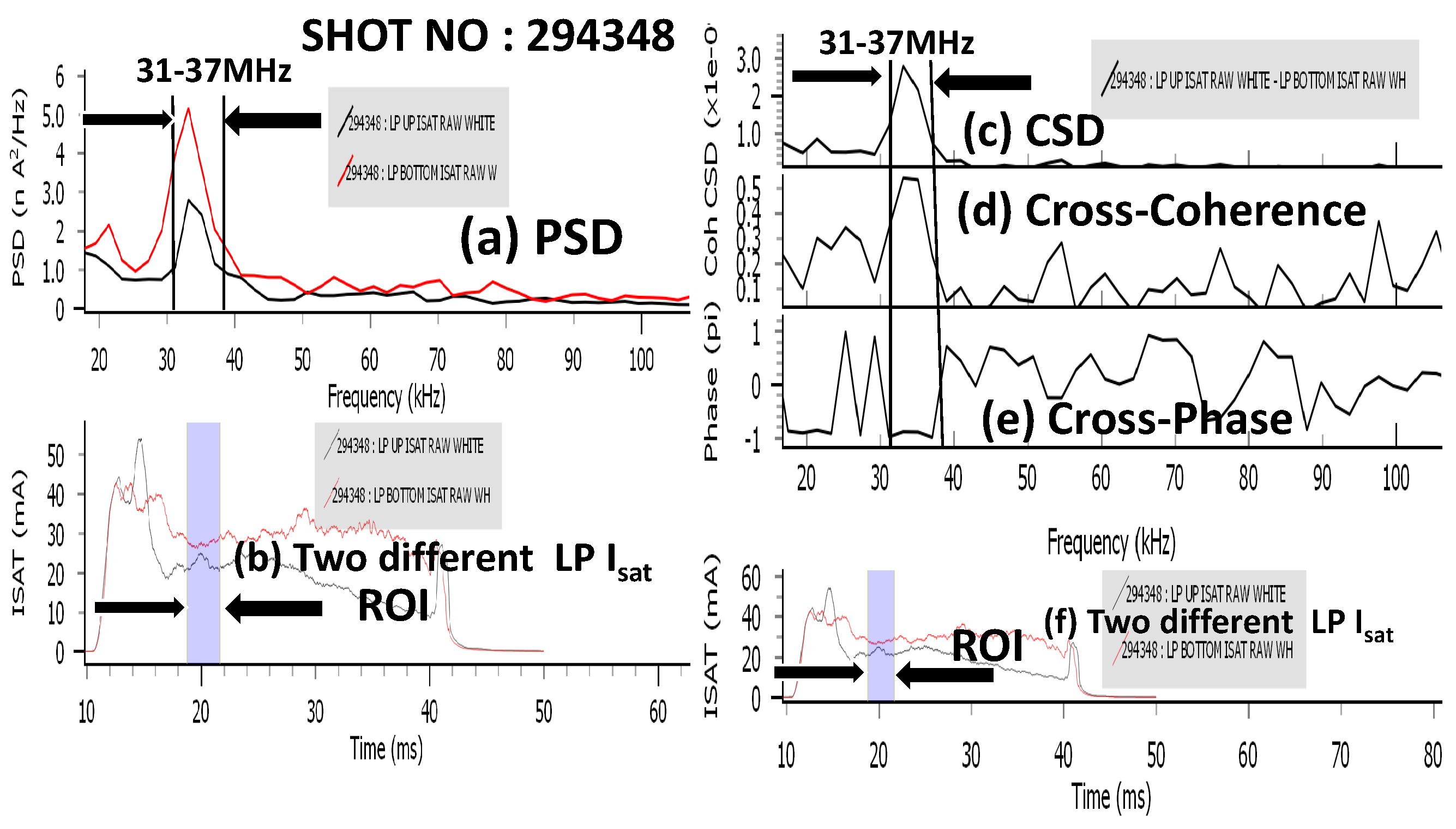
At first, the ROI was taken over the whole flat-top region of $I_{sat}$ signals, collected by the top and bottom Langmuir probes of a typical STOR-M plasma discharge with Shot Number 294,348 to obtain an overall scenario. Figure 6 clearly indicates the presence of GAM at the flat-top where the ROI time window is 22 ms. It shows the GAM-like mode having a frequency width 30–40 MHz in the plasma discharge, which is observed from the “PSD”, “CSD”, “Cross-coherence”, and “Cross-phase”, which are presented in Figure 6a,c–e, respectively. Figure 6b,f present similar $I_{sat}$ signals collected from the “top” and “bottom” Langmuir probes.

The ROI window was set and started to move in different parts of those two top and bottom Langmuir probe $I_{sat}$ signals to characterize and to understand more precisely at which time GAM appears, as well as its time duration. Figure 7 indicates that a clear GAM of frequency width 31–37 MHz emerges around 18.8 ms within a time window of of width of around 2.9 ms, which is clearly marked by the gray rectangular area of the ROI. Here, Figure 7b,f show similar $I_{sat}$ signals collected from the “top” and “bottom” Langmuir probes, which have been smoothed to obtain a clear envelope of those signals. The evolution of the envelopes of signals suggests that they are located approximately on the same magnetic surfaces. The sharp peaks of the “PSD”, “CSD”, “Cross-coherence”, and “Cross-phase”, presented in Figure 7a,c–e, respectively, shows a clear indication of a GAM-like mode when the time range of the ROI is at around 18.8 ms within a time window of around 2.9 ms.

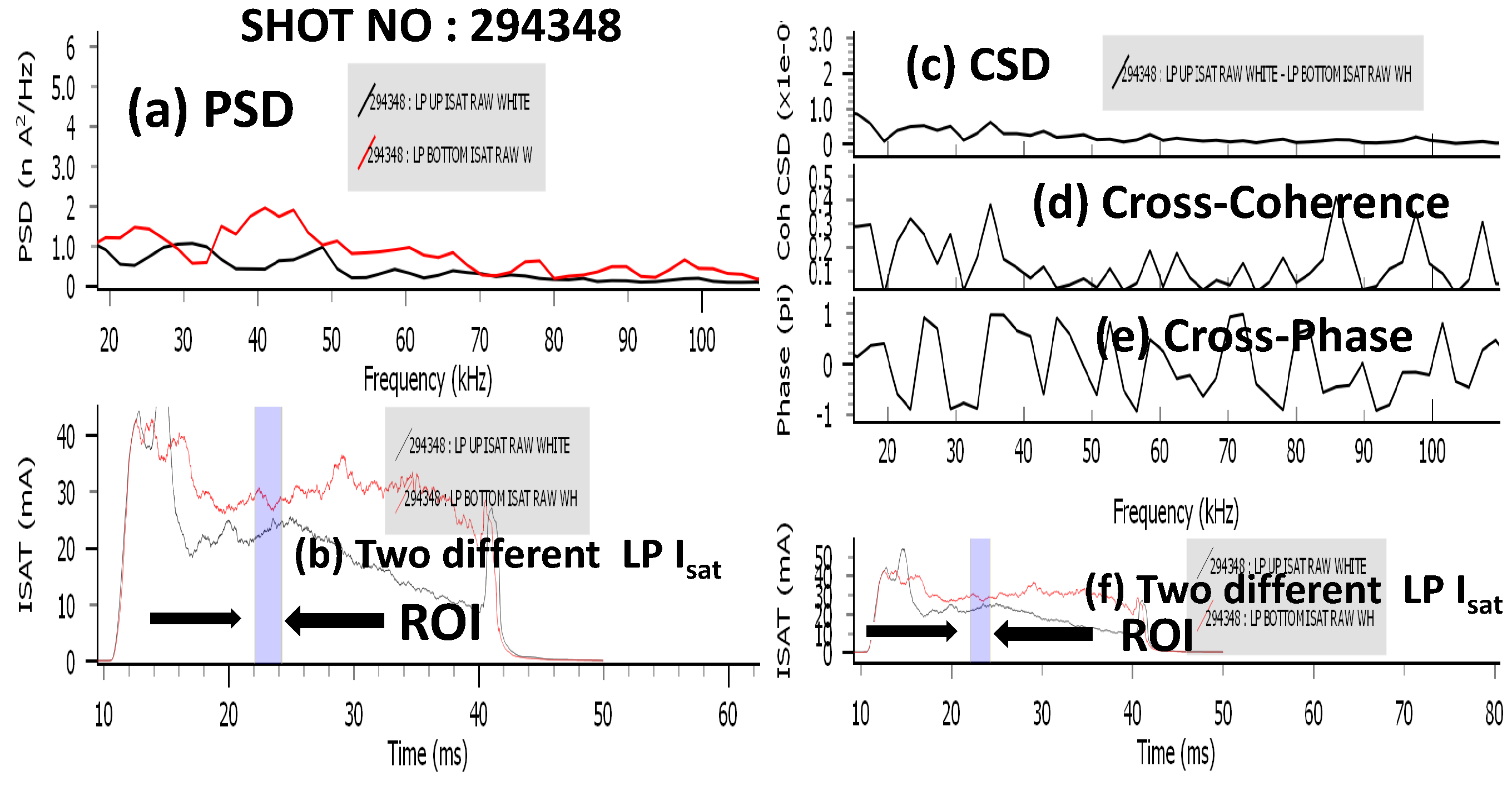
When the ROI window is moved in different locations for the same two signals, it was noticed that the GAM disappears, as shown in Figure 8, for an ROI window within 22–24 ms on the $I_{sat}$ signals, due to the lack of the clear peaks of the GAM-like mode in the “PSD”, “CSD”, “Cross-coherence”, and “Cross-phase”, presented in Figure 8a,c–e, respectively.

Therefore, it is clear that moving the ROI on the signals, we can easily detect GAM very precisely in terms of its time of appearance in the discharge, as well as its existing time duration through the quick and efficient characterizations of GAM.

5. Conclusions and Future Work

It is clear from the previous discussion that this code is highly efficient to analyze and detect the sophisticated GAM-like mode. This code is user friendly through its graphical interface. It has also options to add more analyses or components to its GUI window. Recently, bi-coherence analysis was added to the codes with flexible parameter options such that it can easily calculate higher-order coherence. This addition will be tested and validated soon. In the future, more analytical options related to time series signal processing will be added and will be used for more elaborate and larger scenarios.