A Class of Sparse Direct Broyden Method for Solving Sparse Nonlinear Equations

Abstract

In our paper, we present a sparse quasi-Newton method, called the sparse direct Broyden method, for solving sparse nonlinear equations. The method can be seen as a Broyden-like method and is a least change update satisfying the sparsity condition and direct tangent condition simultaneously. The local and q-superlinear convergence is presented based on the bounded deterioration property and Dennis–Moré condition. By adopting a nonmonotone line search, we establish the global and superlinear convergence. Moreover, the unit step length is essentially accepted. Numerical results demonstrate that the sparse direct Broyden method is effective and competitive for large-scale nonlinear equations.

1. Introduction

We consider the nonlinear equation

$$F\left(x\right)=0,x\in R^n,$$

(1)

where $F:R^n\to R^n$ is a continuously differentiable mapping. We denote $F^{\prime }\left(x\right)$ as the Jacobian matrix of $F\left(x\right)$ at x and pay attention to the case $F^{\prime }\left(x\right)$ having sparse or special structures. Specifically, one has

$$F\left(x\right)={(F_1\left(x\right),F_2\left(x\right),\cdots ,F_n\left(x\right))}^T,$$

and

$$F^{\prime }\left(x\right)={(\nabla F_1\left(x\right),\nabla F_2\left(x\right),\cdots ,\nabla F_n\left(x\right))}^T.$$

Nonlinear equations arise from many scientific and engineering problems and have various applications in the fields such as physics, biology, and many other fields [1].

The linearization of nonlinear Equation (1) at an iterative point $x_k$ is

$$F\left(x\right)\approx F\left(x_k\right)+F^{\prime }\left(x_k\right)(x-x_k)=0;$$

when $F^{\prime }\left(x_k\right)$ is nonsingular, we obtain the Newton–Raphson method

$$x_{k+1}=x_k-F^{\prime }{\left(x_k\right)}^{-1}F\left(x_k\right).$$

Newton’s method is theoretically efficient because it is locally quadratically convergent when the Jacobian matrix is nonsigular and Lipschitz continuous at the solution of $F\left(x\right)$ [2]. However, at each iteration, Newton’s method must compute the exact Jacobian matrix to keep the quadratic convergence rate. The idea of quasi-Newton methods is to approximate the Jacobian matrix $F^{\prime }\left(x_k\right)$ by a quasi-Newtonian matrix $B_k$ with an acceptable reduction of convergence rate. However, at each iteration, Newton’s method must compute the exact Jacobian matrix. To avoid computing the derivatives directly, quasi-Newton methods have been proposed, where $F^{\prime }\left(x_k\right)$ is approximated by a quasi-Newton matrix $B_k\in R^{n\times n}$. Thus, quasi-Newton methods generate an iteration as follows:

$$x_{k+1}=x_k+{\alpha }_k{d}_k,$$

where the step length ${\alpha }_k>0$ is determined by some line search strategies, and $d_k$ is the quasi-Newton direction obtained by solving the subproblem

$$F\left(x_k\right)+B_k{d}_k=0.$$

Usually, as an approximation to the Jacobian matrix $F^{\prime }\left(x_k\right)$, matrix $B_k$ usually satisfies the so-called quasi-Newton condition

$$B_{k+1}{s}_k=y_k,$$

where

$$\begin{array}{ccc}\hfill s_k& =& s_{k+1}-s_k={\alpha }_k{d}_k,\hfill \\ \hfill y_k& =& F\left(x_{k+1}\right)-F\left(x_k\right).\hfill \end{array}$$

The quasi-Newton matrix $B_k$ can be updated by kinds of quasi-Newton update formulae, such as Broyden’s method, Powell’s symmetric Broyden method, BFGS method, and DFP methods [3,4].

Quasi-Newton methods are popular among small and medium-scale problems, since they possess local and superlinear convergence without computing the Jacobian [5,6,7]. However, when the dimension of nonlinear equations is large, the matrix $B_k$ will be dense. Then, the computation and time complexity will be high. There are two considerations to motivate us to consider the sparse quasi-Newton methods for solving sparse nonlinear equations in this paper. One is the fact that there are lots of nonlinear equations with sparse or special Jacobian. Moreover, quasi-Newton methods for solving (1) have a good property that they can maintain the sparse structure of Jacobian matrices. Thus, in this paper, we are interested in constructing a sparse quasi-Newton method for solving sparse nonlinear equations, where the Jacobian matrix $F^{\prime }\left(x_k\right)$ has sparse or special structure. Earlier work on sparse quasi-Newton methods was carried out by Schubert [8] and Toint [9], where Schubert modified Broyden’s method by updating $B_k$ row by row so that the sparsity can be maintained and Toint studied sparse and symmetric quasi-Newton methods. There also have been many kinds of methods for solving large-scale nonlinear systems, such as limited-memory quasi-Newton methods [10,11], partitioned quasi-Newton methods [12,13,14], diagonal quasi-Newton method [15,16], and column updating method [17].

However, the global convergence of quasi-Newton methods for nonlinear equations is a relatively difficult topic, not to mention the dense case. This mainly results from the fact that the quasi-Newton direction may not be a descent direction of the merit function

$$\theta \left(x\right)=\frac{1}{2}{\parallel F\left(x\right)\parallel }^2.$$

Griewank [18] and Li and Fukushima [19] have proposed some line search techniques to establish the global convergence of the quasi-Newton method.

The purpose of our paper is to develop a sparse quasi-Newton method and study its local and global convergence. We consider Broyden’s method

$$B_{k+1}=B_k+\frac{(y_k-B_k{s}_k)s_k^T}{s_k^T{s}_k}.$$

If we replace $y_k$ with $F^{\prime }\left(x_{k+1}\right)s_k$, we can obtain the following update

$$B_{k+1}=B_k+\frac{(F^{\prime }\left(x_{k+1}\right)-B_k)s_k{s}_k^T}{s_k^T{s}_k},$$

which fulfills the direct tangent condition [20,21]

$$B_{k+1}{s}_k=F^{\prime }\left(x_{k+1}\right)s_k.$$

We call the corresponding method the direct Broyden method. Then, we will develop a sparse direct Broyden method, which enjoys the following nice properties: (a) the new sparse quasi-Newton method is a least change update satisfying the direct tangent condition; (b) the proposed method can preserve the sparsity property of the original Jacobian matrix $F^{\prime }\left(x\right)$ exactly; and (c) the sparse direct Broyden method is globally and superlinearly convergent. Presented limited numerical results demonstrate that our algorithm has better performance than Schubert’s method and the direct Broyden method in iteration counts, function evaluation counts, and Broyden’s mean convergence rate.

The paper is organized as follows: in Section 2, we propose a sparse direct Broyden method and list its nice property. For the full step sparse direct Broyden method, local and superlinear convergence is also given. By adopting a nonmonotone line search, we prove the global and superlinear convergence of the method proposed in Section 2. Moreover, after finitely many iterations, the unit step length will always be accepted. In Section 4, we do some preliminary numerical experiments to test the efficiency of the proposed method. In the last section, we give the conclusion.

2. A New Sparse Quasi-Newton Update and Local Convergence

We pay attention to nonlinear Equation (1), whose Jacobian matrix is sparse or has a special structure. Firstly, we introduce some notations to describe the sparsity structure of the Jacobian as that in [22]. Define the sparsity features of the ith row of $F^{\prime }\left(x\right)$

$$V_i=\{v\in R^n:e_j^{T}v=0 \mathrm{for} \mathrm{all} j \mathrm{such} \mathrm{that} {\left(F^{\prime }\left(x\right)\right)}_{ij}=e_i^T{F}^{\prime }\left(x\right)e_j=0 \mathrm{for} \mathrm{all} x\in R^n\},$$

where $e_j$ is the jth column of identity matrix. Then, we can obtain the set of matrices V that preserve the sparsity pattern of $F^{\prime }\left(x\right)$:

$$V=\{A\in R^{n\times n}:A^T{e}_i\in V_i,i=1,2,\cdots ,n\}.$$

Define a projection operator $S_i$, $i=1,2,\dots ,n$, which maps $R^n$ onto $V_i$:

$$\begin{array}{c}\hfill {\left(S_i\left(s_k\right)\right)}_j={\left(s{\left(i\right)}_k\right)}_j=\left\{\begin{array}{cc}{\left(s_k\right)}_j,\hfill & \mathrm{if}{v}_j\ne 0,\\ 0,\hfill & \mathrm{if}{v}_j=0.\end{array}\right.\end{array}$$

Similar to the derivation of Schubert’s method [8], we consider the sparse extension of direct Broyden update [2]

$$B_{k+1}=B_k+\frac{(F^{\prime }\left(x_{k+1}\right)-B_k)s_k{s}_k^T}{s_k^T{s}_k},$$

which fulfills the direct tangent condition

$$B_{k+1}{s}_k=F^{\prime }\left(x_{k+1}\right)s_k.$$

(2)

Then, we can obtain a compact representation of the new sparse quasi-Newton update as

$$B_{k+1}=B_k+\sum _{i=1}^n{\left(s{\left(i\right)}_k^{T}s{\left(i\right)}_k\right)}^{+}{e}_i^T(F^{\prime }\left(x_{k+1}\right)-B_k)s_k{e}_{i}s{\left(i\right)}_k^T,$$

(3)

where the pseudo-inverse of $\alpha \in R$ is defined by

$$\begin{array}{c}\hfill {\alpha }^{+}=\left\{\begin{array}{cc}{\alpha }^{-1},\hfill & \mathrm{if}\alpha \ne 0,\\ 0,\hfill & \mathrm{if}\alpha =0.\end{array}\right.\end{array}$$

The new sparse quasi-Newton method (3) updates the quasi-Newton matrix row by row to preserve the zero and nonzero structure of the Jacobian.

Then, we can obtain a quasi-Newton method as

$$x_{k+1}=x_k+{\alpha }_k{d}_k,$$

where $d_k$ can be obtained by solving the following subproblem

$$F\left(x_k\right)+B_k{d}_k=0,$$

and $B_k$ is updated by sparse direct Broyden update

$$B_{k+1}=B_k+\sum _{i=1}^n{\left(s{\left(i\right)}_k^{T}s{\left(i\right)}_k\right)}^{+}{e}_i^T(F^{\prime }\left(x_{k+1}\right)-B_k)s_k{e}_{i}s{\left(i\right)}_k^T.$$

We call the corresponding method the sparse direct Broyden method. When ${\alpha }_k\equiv 1$, we refer to it as a full step sparse direct Broyden method.

Lemma 1.

The $B_{k+1}$ defined by (3) is the unique solution to the following minimization problem:

$$min\{\parallel B-B_k{\parallel }_F:B\in V\cap Q(F^{\prime }\left(x_{k+1}\right),s_k)\},$$

(4)

where $Q(F^{\prime }\left(x_{k+1}\right),s_k)=\{B\in R^{n\times n}|B{s}_k=F^{\prime }\left(x_{k+1}\right)s_k\}$.

Proof. 

Firstly, we will prove that $B_{k+1}\in V\cap Q(F^{\prime }\left(x_{k+1}\right),s_k)\}$. For $i=1,2,\cdots ,n$, multiply both sides of (3) by $e_i^T$, to obtain

$$e_i^T{B}_{k+1}=e_i^T{B}_k+{\left(s{\left(i\right)}_k^{T}s{\left(i\right)}_k\right)}^{+}{e}_i^T(F^{\prime }\left(x_{k+1}\right)-B_k)s_{k}s{\left(i\right)}_k^T.$$

Since $B_k^T{e}_i\in V_i$ and $s_k\in V_i$, then we have $B_{k+1}^T{e}_i\in V_i$, which implies $B_{k+1}\in V$.

If $s{\left(i\right)}_k\ne \mathbf{0}$, one has

$$e_i^T{B}_{k+1}{s}_k=e_i^T{B}_k{s}_k+{\left(s{\left(i\right)}_k^{T}s{\left(i\right)}_k\right)}^{+}{e}_i^T(F^{\prime }\left(x_{k+1}\right)-B_k)s_{k}s{\left(i\right)}_k^T{s}_k.$$

(5)

According to the definition of the operator $S_i$, we have

$$s{\left(i\right)}_k^{T}s{\left(i\right)}_k=s{\left(i\right)}_k^T{s}_k\mathrm{and}{\left(s{\left(i\right)}_k^{T}s{\left(i\right)}_k\right)}^{+}={\left(s{\left(i\right)}_k^{T}s{\left(i\right)}_k\right)}^{-1}.$$

Then, (5) can be written as

$$e_i^T{B}_{k+1}{s}_k=e_i^T{B}_k{s}_k+e_i^T(F^{\prime }\left(x_{k+1}\right)-B_k)s_k=e_i^T{F}^{\prime }\left(x_{k+1}\right)s_k.$$

If $s{\left(i\right)}_k=\mathbf{0}$, we have

$$e_i^T{F}^{\prime }\left(x_{k+1}\right)s_k=e_i^T{F}^{\prime }\left(x_{k+1}\right)s{\left(i\right)}_k=0,$$

thus $e_i^T{B}_{k+1}{s}_k=e_i^T{F}^{\prime }\left(x_{k+1}\right)s_k$, which implies $B_{k+1}{s}_k=F^{\prime }\left(x_{k+1}\right)s_k$. Therefore, $B_{k+1}\in Q(F^{\prime }\left(x_{k+1}\right),s_k)\}$.

Then, we will prove the uniqueness. Suppose that ${\overline{B}}_{k+1}\in Q(F^{\prime }\left(x_{k+1}\right),s_k)\}$. Since ${\overline{B}}_{k+1}{s}_k=F^{\prime }\left(x_{k+1}\right)s_k$ and $({\overline{B}}_{k+1}-B_k)s_k=({\overline{B}}_{k+1}-B_k)s{\left(i\right)}_k$, one has

$$B_{k+1}=B_k+\sum _{i=1}^n{\left(s{\left(i\right)}_k^{T}s{\left(i\right)}_k\right)}^{+}{e}_i^T({\overline{B}}_{k+1}-B_k)s_k{e}_{i}s{\left(i\right)}_k^T.$$

Taking the Frobenius norm,

$$\begin{array}{ccc}\hfill \parallel B_{k+1}-B_k{\parallel }_F& =& {\left(\sum _{i=1}^n{\parallel e_i^T(B_{k+1}-B_k)\parallel }^2\right)}^{1/2}\hfill \\ & =& {\left(\sum _{i=1}^n{\parallel {\left(s{\left(i\right)}_k^{T}s{\left(i\right)}_k\right)}^{+}{e}_i^T({\overline{B}}_{k+1}-B_k)s_{k}s{\left(i\right)}_k^T\parallel }^2\right)}^{1/2}\hfill \\ & =& {\left(\sum _{i=1}^n|{\left(s{\left(i\right)}_k^{T}s{\left(i\right)}_k\right)}^{+}{e}_i^T({\overline{B}}_{k+1}-B_k)s{\left(i\right)}_k{|}^2·{\parallel s{\left(i\right)}_k\parallel }^2\right)}^{1/2}\hfill \\ & \le & {\left(\sum _{i=1,s{\left(i\right)}_k\ne \mathbf{0}}^n{\parallel e_i^T({\overline{B}}_{k+1}-B_k)\parallel }^2\right)}^{1/2}\hfill \\ & \le & {\left(\sum _{i=1}^n{\parallel e_i^T({\overline{B}}_{k+1}-B_k)\parallel }^2\right)}^{1/2}\hfill \\ & =& \parallel {\overline{B}}_{k+1}-B_k{\parallel }_F,\hfill \end{array}$$

where the first inequality follows from the triangle inequality. Since the function $f\left(B\right)=\parallel B-B_k{\parallel }_F$ is strictly convex and the constraint condition (4) is convex, we can obtain the uniqueness.    □

To analyze the local convergence of the full step sparse direct Broyden method, first we show that the bounded deterioration property

$$\parallel B_{k+1}-F^{\prime }\left(x^{*}\right){\parallel }_F\le (1+{\alpha }_1{\sigma }_k){\parallel B_k-F^{\prime }\left(x^{*}\right)\parallel }_F+{\alpha }_2{\gamma }_k,$$

(6)

is satisfied with some constants ${\alpha }_1,{\alpha }_2\ge 0$, where ${\gamma }_k=max\{\parallel x_k-x^{*}{\parallel }_2,\parallel x_{k+1}-x^{*}{{\parallel }_2\}}^2$.

Lemma 2.

Suppose that $F:R^n\to R^n$ is continuously differentiable in $D_0$, which is an open and convex set. Let $x^{*}\in D_0$ be a solution of (1) at which $F^{\prime }\left(x^{*}\right)$ is nonsingular. Suppose that there exists $K=(k_1,k_2,\cdots ,k_n)\in R^n$ with $k_i\ge 0$, for $i=1,2,\dots ,n$, such that

$$\parallel e_i^T(F^{\prime }\left(x\right)-F^{\prime }\left(y\right))\parallel \le k_i\parallel x-y\parallel ,\forall x,y\in D_0.$$

Then, one has the estimation

$$\parallel B_{k+1}-F^{\prime }\left(x^{*}\right){\parallel }_F^2\le {\parallel B_k-F^{\prime }\left(x^{*}\right)\parallel }_F^2-\frac{\parallel (B_k-F^{\prime }\left(x^{*}\right))s_k{\parallel }^2}{\parallel s_k{\parallel }^2}+L^2{\gamma }_k,$$

where $L={\parallel K\parallel }_2$.

Proof. 

For the case $s_k=\mathbf{0}$, then it is obvious that $F\left(x_k\right)=\mathbf{0}$ and $x_k=x^{*}$. For the case $s_k\ne \mathbf{0}$, subtracting $F^{\prime }\left(x^{*}\right)$ from both sides of the update formula

$$B_{k+1}=B_k+\sum _{i=1}^n{\left(s{\left(i\right)}_k^{T}s{\left(i\right)}_k\right)}^{+}{e}_i^T(F^{\prime }\left(x_{k+1}\right)-B_k)s_k{e}_{i}s{\left(i\right)}_k^T,$$

and multiplying by $e_i^T$, $i=1,2,\cdots ,n$, one has

$$\begin{array}{ccc}& & e_i^T(B_{k+1}-F^{\prime }\left(x^{*}\right))\hfill \\ & =& e_i^T(B_k-F^{\prime }\left(x^{*}\right))+{\left(s{\left(i\right)}_k^{T}s{\left(i\right)}_k\right)}^{+}{e}_i^T(F^{\prime }\left(x_{k+1}\right)-B_k)s_{k}s{\left(i\right)}_k^T\hfill \\ & =& e_i^T(B_k-F^{\prime }\left(x^{*}\right))(I-{\left(s{\left(i\right)}_k^{T}s{\left(i\right)}_k\right)}^{+}s{\left(i\right)}_{k}s{\left(i\right)}_k^T)\hfill \\ & & +{\left(s{\left(i\right)}_k^{T}s{\left(i\right)}_k\right)}^{+}{e}_i^T(F^{\prime }\left(x_{k+1}\right)-F^{\prime }\left(x^{*}\right))s_{k}s{\left(i\right)}_k^T.\hfill \end{array}$$

Taking norms yields

$$\begin{array}{ccc}\hfill & & \parallel e_i^T(B_{k+1}-F^{\prime }\left(x^{*}\right)){\parallel }_F^2\hfill \\ & =& \parallel e_i^T(B_k-F^{\prime }\left(x^{*}\right))(I-{\left(s{\left(i\right)}_k^{T}s{\left(i\right)}_k\right)}^{+}s{\left(i\right)}_{k}s{\left(i\right)}_k^T){\parallel }^2\hfill \\ & & +{\left(s{\left(i\right)}_k^{T}s{\left(i\right)}_k\right)}^{+}{\left|e_i^T(F^{\prime }\left(x_{k+1}\right)-F^{\prime }\left(x^{*}\right))s_k\right|}^2\hfill \\ & =& \parallel e_i^T(B_k-F^{\prime }\left(x^{*}\right)){\parallel }_2^2-{\left(s{\left(i\right)}_k^{T}s{\left(i\right)}_k\right)}^{+}{\left|e_i^T{E}_{k}s{\left(i\right)}_k\right|}^2\hfill \\ & & +{\left(s{\left(i\right)}_k^{T}s{\left(i\right)}_k\right)}^{+}{\left|e_i^T(F^{\prime }\left(x_{k+1}\right)-F^{\prime }\left(x^{*}\right))s_k\right|}^2\hfill \\ & \le & \parallel e_i^T{E}_k{\parallel }_2^2-\frac{|e_i^T{E}_k{s}_k{|}^2}{\parallel s_k{\parallel }^2}+{\left(s{\left(i\right)}_k^{T}s{\left(i\right)}_k\right)}^{+}{\left|e_i^T(F^{\prime }\left(x_{k+1}\right)-F^{\prime }\left(x^{*}\right))s_k\right|}^2.\hfill \end{array}$$

(7)

If $s{\left(i\right)}_k=\mathbf{0}$, then we have ${\left(s{\left(i\right)}_k^{T}s{\left(i\right)}_k\right)}^{+}=0$. It is obvious that

$$0={\left(s{\left(i\right)}_k^{T}s{\left(i\right)}_k\right)}^{+}{\left|e_i^T(F^{\prime }\left(x_{k+1}\right)-F^{\prime }\left(x^{*}\right))s_k\right|}^2\le k_i^2{\sigma }_k.$$

If $s{\left(i\right)}_k\ne \mathbf{0}$, it follows that

$$\begin{array}{c}{\displaystyle {\left(s{\left(i\right)}_k^{T}s{\left(i\right)}_k\right)}^{+}{\left|e_i^T(F^{\prime }\left(x_{k+1}\right)-F^{\prime }\left(x^{*}\right))s_k\right|}^2}\\ =\hspace{1em}{\left(s{\left(i\right)}_k^{T}s{\left(i\right)}_k\right)}^{+}{\left|e_i^T(F^{\prime }\left(x_{k+1}\right)-F^{\prime }\left(x^{*}\right))s{\left(i\right)}_k\right|}^2\hfill \\ \le \hspace{1em}\parallel e_i^T(F^{\prime }\left(x_{k+1}\right)-F^{\prime }\left(x^{*}\right)){\parallel }^2\hfill \\ \le \hspace{1em}{k}_i^2{\parallel x_{k+1}-x^{*}\parallel }^2\hfill \\ \le \hspace{1em}{k}_i^2{\sigma }_k^2.\hfill \end{array}$$

Thus, (7) reduces to

$$\parallel e_i^T(B_{k+1}-F^{\prime }\left(x^{*}\right)){\parallel }_F^2\le {\parallel e_i^T(B_k-F^{\prime }\left(x^{*}\right))\parallel }^2-\frac{|e_i^T(B_k-F^{\prime }\left(x^{*}\right))s_k{|}^2}{\parallel s_k{\parallel }^2}+k_i^2{\gamma }_k,$$

Make a summation to obtain

$$\parallel (B_{k+1}-F^{\prime }\left(x^{*}\right)){\parallel }_F^2\le {\parallel (B_k-F^{\prime }\left(x^{*}\right))\parallel }_F^2-\frac{\parallel (B_k-F^{\prime }\left(x^{*}\right))s_k{\parallel }^2}{\parallel s_k{\parallel }^2}+L^2{\gamma }_k.$$

(8)

   □

Based on the classical framework of Dennis and Moré, we give the following local convergence, which can be proved similar to the case of Broyden’s method [6,7].

Theorem 1.

Let the conditions in Lemma 2 hold. Then, there exist constants $ϵ,\delta >0$ such that, if $\parallel x_0-x^{*}{\parallel }_2<ϵ$ and $\parallel B_0-F^{\prime }\left(x^{*}\right){\parallel }_F<\delta$, the sequence $\left\{x_k\right\}$ is well defined and converges to $x^{*}$. Furthermore, the convergence rate is superlinear.

Proof. 

According to Lemma 2, one has

$$\parallel (B_{k+1}-F^{\prime }\left(x^{*}\right)){\parallel }_F\le \parallel (B_k-F^{\prime }\left(x^{*}\right){\parallel }_F+L{\gamma }_k,$$

which means that the estimation (6) is satisfied with ${\alpha }_1=0$ and ${\alpha }_2=L$. Then, we obtain the local and linear convergence of $\left\{x_k\right\}$.

Next, we will show the Dennis–Moré condition [7]

$$\underset{k\to \infty }{lim}\frac{\parallel (B_k-F^{\prime }\left(x^{*}\right))s_k\parallel }{\parallel s_k\parallel }=0$$

(9)

is satisfied. According to (8), one has

$$\parallel (B_{k+1}-F^{\prime }\left(x^{*}\right)){\parallel }_F\le {\left(\parallel (B_k-F^{\prime }\left(x^{*}\right)){\parallel }_F^2-\frac{\parallel (B_k-F^{\prime }\left(x^{*}\right))s_k{\parallel }^2}{\parallel s_k{\parallel }^2}\right)}^{1/2}+L{\gamma }_k;$$

then, the result can be proved similar to that in [7].    □

3. Algorithm and Global Convergence

In this section, by the use of LF condition [19], we propose a global sparse Broyden method, whose specific steps are listed in the following  Algorithm 1.

Algorithm 1 (Sparse direct Broyden Method for solving sparse nonlinear equations)

Step 0. Given constant ${\sigma }_1,{\sigma }_2>0$ and $\rho ,r\in (0,1)$. Given a positive sequence $\left\{{\eta }_k\right\}$ satisfying $$\sum _{k=0}^{\infty }{\eta }_k\le \eta <\infty .$$ (10) Given $x_0\in R^n$, stop tolerance $ϵ>0$, and a nonsingular matrix $B_0\in R^{n\times n}$. Set $k:=0$. Step 1. Stop if $\parallel F\left(x_k\right)\parallel \le ϵ$. Step 2. Solve the subproblem $$F\left(x_k\right)+B_k{d}_k=0$$ (11) to obtain the quasi-Newton direction $d_k$. Step 3. If  $$\parallel F(x_k+d_k)\parallel \le \rho \parallel F\left(x_k\right)\parallel -{\sigma }_1{\parallel d_k\parallel }^2,$$ (12) then let ${\alpha }_k:=1$ and go to Step 5. Else, go to Step 4. Step 4. Set ${\alpha }_k=r^{i_k}$, where $i_k$ is the smallest nonnegative integer i satisfying $$\parallel F(x_k+r^i{d}_k)\parallel \le \parallel F\left(x_k\right)\parallel -{\sigma }_2\parallel r^i{d}_k{\parallel }^2+{\eta }_k\parallel F\left(x_k\right)\parallel ,$$ (13) where ${\eta }_k$ is defined as in (10). Step 5. Set $x_{k+1}:=x_k+{\alpha }_k{d}_k$. Step 6. Update $B_k$ to obtain $B_{k+1}$ by sparse direct Broyden update $$B_{k+1}=B_k+\sum _{i=1}^n{\left(s{\left(i\right)}_k^{T}s{\left(i\right)}_k\right)}^{+}{e}_i^T(F^{\prime }\left(x_{k+1}\right)-B_k)s_k{e}_{i}s{\left(i\right)}_k^T,$$ (14) Set $k:=k+1$. Go to Step 1.

Remark 1.

It is noticed that the update formula (14) may be singular when $B_k$ is nonsingular. In this case, we use a similar technique in [22,23] and give the following discussion about the nonsingular sparse direct Broyden update.

Set $H_0=B_k$, and for $i=1,2,\dots ,n$, let

$$\begin{array}{ccc}\hfill H_i& =& H_0+\sum _{j=1}^i{\theta }_k^j{\left(s{\left(j\right)}_k^{T}s{\left(j\right)}_k\right)}^{+}{e}_j^T(F^{\prime }\left(x_{k+1}\right)-B_k)s_k{e}_{j}s{\left(j\right)}_k^T\hfill \\ & =& H_{i-1}+{\theta }_k^i{\left(s{\left(i\right)}_k^{T}s{\left(i\right)}_k\right)}^{+}{e}_i^T(F^{\prime }\left(x_{k+1}\right)-B_k)s_k{e}_{i}s{\left(i\right)}_k^T.\hfill \end{array}$$

Since $e_i^T{H}_0=e_i^T{H}_1=\cdots =e_i^T{H}_{i-1}$, then

$$H_i=H_{i-1}+{\theta }_k^i{\left(s{\left(i\right)}_k^{T}s{\left(i\right)}_k\right)}^{+}{e}_i^T(F^{\prime }\left(x_{k+1}\right)-H_{i-1})s_k{e}_{i}s{\left(i\right)}_k^T.$$

For a scalar $\alpha \in (0,1)$, ${\theta }_k^i$ can be chosen such that

$$\mid det{H}_i\mid \ge \mid \sqrt[n]{\alpha }\mid det{H}_{i-1}\mid ,{\theta }_k^i\in \left[\frac{1-\sqrt[n]{\alpha }}{1+\sqrt[n]{\alpha }},1\right].$$

Thus, $\mid det{B}_{k+1}\mid \ge \alpha \mid det{B}_k\mid$ and ${\theta }_k^i$ can be chosen so that

$$B_{k+1} is nonsigular,and\mid {\theta }_k^i-1\mid \le \widehat{\theta }<1.$$

Thus, we can define the sparse direct Broyden-like update formula as

$$B_{k+1}=B_k+\sum _{i=1}^n{\theta }_k^i{\left(s{\left(i\right)}_k^{T}s{\left(i\right)}_k\right)}^{+}{e}_i^T(F^{\prime }\left(x_{k+1}\right)-B_k)s_k{e}_{i}s{\left(i\right)}_k^T.$$

Remark 2.

It can be seen that the update formula (14) includes $F^{\prime }\left(x_{k+1}\right)$, but it does not need to compute $F^{\prime }\left(x_{k+1}\right)$ in practice. Automatic differentiation is a chain-rule-based technique for evaluating the derivatives with respect to the input variables of functions defined by a high-level computer program. Automatic Differentiation has two basic modes of operations, the forward mode and the reverse mode. In the forward mode, the derivatives are propagated throughout the computation using the chain rule, while in the reverse mode the adjoint derivatives are propagated backwards. The forward mode and reverse mode of automatic differentiation provide the possibility to compute $F^{\prime }\left(x\right)s$ and ${\sigma }^T{F}^{\prime }\left(x\right)$ exactly within machine accuracy for given vectors $x,s$ and σ.

  To establish the global convergence, we need the following conditions.

Assumption 1.

(1)

F is continuously differentiable on Ω, which is a bounded level set defined by

$$\Omega =\{x\in R^n\mid \parallel F\left(x\right)\parallel \le e^{\eta }\parallel F\left(x_0\right)\parallel \}.$$

(2)

$F^{\prime }\left(x\right)$ is Lipschitz continuous on Ω with Lipschitz constant $L>0$

$$\parallel F^{\prime }\left(x\right)-F^{\prime }\left(y\right)\parallel \le L\parallel x-y\parallel ,\forall x,y\in \Omega .$$

(3)

$F^{\prime }\left(x\right)$ is nonsingular for any $x\in \Omega$.

   First, we give the following important lemmas.

Lemma 3.

The sequence $\left\{x_k\right\}$ generated by Algorithm 1 is contained in Ω. Moreover, it holds that

$$\sum _{k=0}^{\infty }{\parallel s_k\parallel }^2<\infty ,$$

(15)

and the sequence $\{\parallel F\left(x_k\right)\parallel \}$ converges.

Proof. 

According to the line search (12) and (13), one has for any k

$$\begin{array}{ccc}\hfill \parallel F\left(x_{k+1}\right)\parallel & \le & (1+{\eta }_k)\parallel F\left(x_k\right)\parallel \hfill \\ & ⋮& \\ & \le & \parallel F\left(x_0\right)\parallel \left[{\Pi }_{j=0}^k(1+{\eta }_j)\right]\hfill \\ & \le & \parallel F\left(x_0\right)\parallel {\left[\frac{1}{k+1}\sum _{j=0}^k(1+{\eta }_j)\right]}^{k+1}\hfill \\ & =& \parallel F\left(x_0\right)\parallel {\left[1+\frac{1}{k+1}\sum _{j=0}^k{\eta }_j\right]}^{k+1}\hfill \\ & \le & \parallel F\left(x_0\right)\parallel {\left[{\left(1+\frac{\eta }{k+1}\right)}^{\frac{k+1}{\eta }}\right]}^{\eta }\hfill \\ & \le & e^{\eta }\parallel F\left(x_0\right)\parallel .\hfill \end{array}$$

Thus, $\left\{x_k\right\}$ is contained in level set $\Omega$. Moreover, the sequence $\{\parallel F\left(x_k\right)\parallel \}$ is bounded.

On the basis of (12) and (13), we have for each k that

$${\sigma }_0\parallel s_k{\parallel }^2={\sigma }_0\parallel x_{k+1}-x_k{\parallel }^2\le \parallel F\left(x_k\right)\parallel -\parallel F\left(x_{k+1}\right)\parallel +{\eta }_k\parallel F_k\parallel ,$$

where ${\sigma }_0=min\{{\sigma }_1,{\sigma }_2\}$. We can obtain (15) by taking summation on both sides for k from 0 to ∞.

Finally, since $\{\parallel F\left(x_k\right)\parallel \}$ satisfies

$$\parallel F(x_k+{\alpha }_k{d}_k)\parallel \le (1+{\eta }_k)\parallel F\left(x_k\right)\parallel ,$$

and $\left\{{\eta }_k\right\}$ satisfies

$$\sum _{k=0}^{\infty }{\eta }_k\le \eta <\infty ,$$

we then obtain the convergence of $\{\parallel F\left(x_k\right)\parallel \}$. □

  Denote

$${\delta }_k=\frac{\parallel (F^{\prime }\left(x_{k+1}\right)-B_k)s_k\parallel }{\parallel s_k\parallel }=\frac{\parallel F^{\prime }\left(x_{k+1}\right)s_k+F\left(x_k\right)\parallel }{\parallel s_k\parallel }.$$

Lemma 4.

Suppose that the sequence $\left\{x_k\right\}$ is generated by Algorithm 1, and $F^{\prime }\left(x\right)$ is Lipschitz continuous with a common Lipschitz constant $L>0$. If

$$\sum _{k=0}^{\infty }{\parallel s_k\parallel }^2<\infty ,$$

then we have

$$\underset{t\to \infty }{lim}\frac{1}{t}\sum _{k=0}^{t-1}{\delta }_k^2=0.$$

(16)

In addition, there exists a subsequence of $\left\{{\delta }_k\right\}$ tending to zero. If

$$\sum _{k=0}^{\infty }\parallel s_k\parallel <\infty ,$$

then we have

$$\sum _{k=0}^{\infty }{\delta }_k^2<\infty .$$

(17)

In addition, the whole sequence $\left\{{\delta }_k\right\}$ converges to zero.

Proof. 

According to the update (14), we have

$$e_i^T{B}_{k+1}=e_i^T{B}_k+{\left(s{\left(i\right)}_k^{T}s{\left(i\right)}_k\right)}^{+}{e}_i^T(F^{\prime }\left(x_{k+1}\right)-B_k)s_{k}s{\left(i\right)}_k^T.$$

Subtracting $e_i^T{F}^{\prime }\left(x_{k+1}\right)$, we obtain

$$\begin{array}{ccc}& & {\displaystyle e_i^T(B_{k+1}-F^{\prime }\left(x_{k+1}\right))}\hfill \\ & =& e_i^T(B_k-F^{\prime }\left(x_{k+1}\right))+{\left(s{\left(i\right)}_k^{T}s{\left(i\right)}_k\right)}^{+}{e}_i^T(F^{\prime }\left(x_{k+1}\right)-B_k)s_{k}s{\left(i\right)}_k^T\hfill \\ & =& e_i^T(B_k-F^{\prime }\left(x_{k+1}\right))\left(I-{\left(s{\left(i\right)}_k^{T}s{\left(i\right)}_k\right)}^{+}{s}_{k}s{\left(i\right)}_k^T\right)\hfill \\ & =& e_i^T(B_k-F^{\prime }\left(x_{k+1}\right))\left(I-{\left(s{\left(i\right)}_k^{T}s{\left(i\right)}_k\right)}^{+}s{\left(i\right)}_{k}s{\left(i\right)}_k^T\right).\hfill \end{array}$$

Taking norms yields

$$\begin{array}{ccc}& & {\displaystyle \parallel e_i^T(B_{k+1}-F^{\prime }\left(x_{k+1}\right)){\parallel }^2}\hfill \\ & =& \parallel e_i^T(B_k-F^{\prime }\left(x_{k+1}\right))(I-{\left(s{\left(i\right)}_k^{T}s{\left(i\right)}_k\right)}^{+}s{\left(i\right)}_{k}s{\left(i\right)}_k^T){\parallel }^2\hfill \\ & =& \parallel e_i^T(B_k-F^{\prime }\left(x_{k+1}\right)){\parallel }^2-{\left(s{\left(i\right)}_k^{T}s{\left(i\right)}_k\right)}^{+}{\left(e_i^T(B_k-F^{\prime }\left(x_{k+1}\right))s_k\right)}^2\hfill \\ & \le & \parallel e_i^T(B_k-F^{\prime }\left(x_{k+1}\right)){\parallel }^2-\frac{\parallel e_i^T(B_k-F^{\prime }\left(x_{k+1}\right))s_k{\parallel }^2}{\parallel s_k{\parallel }^2}.\hfill \end{array}$$

Since $\parallel B_{k+1}-F^{\prime }\left(x_{k+1}\right){\parallel }_F^2={\sum }_{i=1}^n{\parallel e_i^T(B_{k+1}-F^{\prime }\left(x_{k+1}\right))\parallel }^2$, making summation from $i=1$ to n yields

$$\begin{array}{ccc}& & \parallel B_{k+1}-F^{\prime }\left(x_{k+1}\right){\parallel }_F^2\hfill \\ & \le & \sum _{i=1}^n\left(\parallel e_i^T(B_k-F^{\prime }\left(x_{k+1}\right)){\parallel }^2-\frac{\parallel e_i^T(B_k-F^{\prime }\left(x_{k+1}\right))s_k{\parallel }^2}{\parallel s_k{\parallel }^2}\right)\hfill \\ & =& \parallel (B_k-F^{\prime }\left(x_{k+1}\right)){\parallel }_F^2-\frac{\parallel (B_k-F^{\prime }\left(x_{k+1}\right))s_k{\parallel }^2}{\parallel s_k{\parallel }^2}\hfill \\ & =& \parallel (B_k-F^{\prime }\left(x_{k+1}\right)){\parallel }_F^2-{\delta }_k^2.\hfill \end{array}$$

Denote

$$D_k=B_k-F^{\prime }\left(x_k\right)\mathrm{and} E_k=F^{\prime }\left(x_{k+1}\right)-F^{\prime }\left(x_k\right).$$

Then, one has that, for $k\ge 1$,

$$\begin{array}{ccc}\hfill \parallel D_k{\parallel }_F& \le & \parallel B_{k-1}-F^{\prime }\left(x_k\right){\parallel }_F\le \parallel D_{k-1}{\parallel }_F+{\parallel E_{k-1}\parallel }_F\hfill \\ & \le & \cdots \le \parallel D_0{\parallel }_F+\sum _{j=0}^{k-1}{\parallel E_j\parallel }_F,\hfill \end{array}$$

and

$$\begin{array}{ccc}\hfill {\delta }_k^2& \le & \parallel B_k-F^{\prime }{(}_{k+1}){\parallel }_F^2-{\parallel B_{k+1}-F^{\prime }\left(x_{k+1}\right)\parallel }_F^2\hfill \\ & =& \parallel D_k-E_k{\parallel }_F-{\parallel D_{k+1}\parallel }_F^2\hfill \\ & \le & \parallel D_k{\parallel }_F^2-\parallel D_{k+1}{\parallel }_F^2+\parallel E_k{\parallel }_F^2+2\parallel E_k{\parallel }_F{\parallel D_k\parallel }_F\hfill \\ & \le & \parallel D_k{\parallel }_F^2-\parallel D_{k+1}{\parallel }_F^2+\parallel E_k{\parallel }_F^2+2{\parallel E_k\parallel }_F·\left(\parallel D_0{\parallel }_F+\sum _{j=0}^{k-1}{\parallel E_j\parallel }_F\right).\hfill \end{array}$$

Making summation on both sides from $k=0$ to $t-1$, we have for $1\le p<t$

$$\begin{array}{ccc}\hfill \sum _{k=1}^{t-1}{\delta }_k^2& \le & \parallel D_0{\parallel }_F^2+\sum _{k=0}^{t-1}\parallel E_k{\parallel }_F^2+2\sum _{k=1}^{t-1}{\parallel E_k\parallel }_F\left(\parallel D_0{\parallel }_F+\sum _{j=0}^{k-1}{\parallel E_j\parallel }_F\right)\hfill \\ & \le & \parallel D_0{\parallel }_F^2+\sum _{k=0}^{t-1}\parallel E_k{\parallel }_F^2+2\parallel D_0{\parallel }_F\sum _{k=1}^{t-1}\parallel E_k{\parallel }_F+2\sum _{k=1}^{t-1}\parallel E_k{\parallel }_F\sum _{j=0}^{k-1}{\parallel E_j\parallel }_F\hfill \\ & =& \parallel D_0{\parallel }_F^2+2\parallel D_0{\parallel }_F^2\sum _{k=1}^{t-1}{\parallel E_k\parallel }_F+2{\left(\sum _{k=1}^{t-1}{\parallel E_k\parallel }_F\right)}^2\hfill \\ & =& {\left(\parallel D_0{\parallel }_F+\sum _{k=0}^{t-1}{\parallel E_k\parallel }_F\right)}^2\hfill \\ & \le & {\left(\parallel D_0{\parallel }_F+\sum _{k=0}^{p-1}\parallel E_k{\parallel }_F+\sum _{k=p}^{t-1}{\parallel E_k\parallel }_F\right)}^2\hfill \\ & \le & 2{\left(\parallel D_0{\parallel }_F+\sum _{k=0}^{p-1}{\parallel E_k\parallel }_F\right)}^2+2{\left(\sum _{k=p}^{t-1}{\parallel E_k\parallel }_F\right)}^2\hfill \\ & \le & 2{\left(\parallel D_0{\parallel }_F+\sum _{k=0}^{p-1}{\parallel E_k\parallel }_F\right)}^2+2(t-p)\sum _{k=p}^{t-1}{\parallel E_k\parallel }_F^2.\hfill \end{array}$$

(18)

Dividing both sides by t and letting $t\to \infty$, we have

$$\underset{t\to \infty }{lim}\frac{1}{t}\sum _{k=1}^{t-1}{\delta }_k^2\le 2\underset{t\to \infty }{lim}\frac{t-p}{t}\sum _{k=p}^{t-1}\parallel E_k{\parallel }_F^2\le 2\sum _{k=p}^{\infty }{\parallel E_k\parallel }_F^2.$$

If ${\sum }_{k=0}^{\infty }{\parallel s_k\parallel }^2<\infty$, then the Lipschitz continuity of $F^{\prime }\left(x\right)$ together with the last inequality implies

$$\underset{t\to \infty }{lim}\frac{1}{t}\sum _{k=0}^{t-1}{\delta }_k^2=0.$$

Then, there is a subsequence of $\left\{{\delta }_k\right\}$ tending to zero. If ${\sum }_{k=0}^{\infty }\parallel s_k\parallel <\infty$, then (17) comes from (18). Moreover, the whole sequence $\left\{{\delta }_k\right\}$ converges to zero. This completes the proof. □

Theorem 2.

Let the conditions in Assumption 1 hold. Then, the sequence $\left\{x_k\right\}$ generated by Algorithm 1 converges to the unique solution $x^{*}$ of (1).

Proof. 

We first verify

$$\underset{k\to \infty }{lim}inf\parallel F\left(x_k\right)\parallel =0.$$

(19)

According to Lemma 3, the sequence $\{\parallel F\left(x_k\right)\parallel \}$ converges. Thus, we only need to prove that there is an accumulation point of $\left\{x_k\right\}$, which is the unique solution of (1). If there are infinitely many ${\alpha }_k$, which is obtained by the line search condition (12), then

$$\parallel F\left(x_{k+1}\right)\parallel \le \rho \parallel F\left(x_k\right)\parallel$$

holds for infinitely many k. This indicates ${lim\; inf}_{k\to \infty }\parallel F\left(x_k\right)\parallel =0$.

There are only finite many ${\alpha }_k$, which is obtained by the line search condition (12). By (15) and Lemma 4, there is a subsequence ${\left\{{\delta }_k\right\}}_{k\in K}$ converging to zero. Since ${\left\{x_k\right\}}_K$ is bounded, we may assume that ${\left\{x_k\right\}}_K\to x^{*}$ without loss of generality. Hence, $\left\{F^{\prime }\left(x_{k+1}\right)\right\}$ tends to $F^{\prime }\left(x^{*}\right)$, and there exists a constant $C_1$ such that $\parallel F^{\prime }\left(x_{k+1}\right)\parallel \le C_1$ for all sufficiently large $k\in K$. According to the subproblem (11) and the definition of ${\delta }_k$, one has

$$\begin{array}{ccc}\hfill \parallel d_k\parallel & =& \parallel F^{\prime }{\left(x_{k+1}\right)}^{-1}((F^{\prime }\left(x_{k+1}\right)-B_k)d_k-F\left(x_k\right))\parallel \hfill \\ & \le & \parallel F^{\prime }{\left(x_{k+1}\right)}^{-1}\parallel \left(\parallel (F^{\prime }\left(x_{k+1}\right)-B_k)d_k\parallel +\parallel F\left(x_k\right)\parallel \right)\hfill \\ & \le & C_1({\delta }_k\parallel d_k\parallel +\parallel F\left(x_k\right)\parallel ),\hfill \end{array}$$

which indicates that there exists a constant $M_1$ such that

$$\parallel d_k\parallel \le M_1\parallel F\left(x_k\right)\parallel$$

holds for all sufficiently large $k\in K$. Thus, the subsequence ${\left\{d_k\right\}}_K$ is bounded, and we can assume that ${\left\{d_k\right\}}_K\to d^{*}$. Since $\parallel (F^{\prime }\left(x_{k+1}\right)-B_k)d_k\parallel ={\delta }_k\parallel d_k\parallel$, then we have

$$B_k{d}_k\to F^{\prime }\left(x^{*}\right)d^{*},k\to \infty ,k\in K.$$

Taking limit in the subproblem (11) as $k\to \infty ,k\in K$, one has

$$F^{\prime }\left(x^{*}\right)d^{*}+F\left(x^{*}\right)=0.$$

(20)

Denote ${\alpha }^{*}={lim\; sup}_{k\to \infty ,k\in K}{\alpha }_k$. It is clear that ${\alpha }^{*}\ge 0$ and ${\alpha }^{*}{d}^{*}=0$. If $\overline{\alpha }>0$, then $d^{*}=0$; hence, it follows from (20) that $F\left(x^{*}\right)=0$. If ${\alpha }^{*}=0$, or equivalently ${lim}_{k\to \infty }{\alpha }_k=0$. According to the line search rule, when $k\in K$ is sufficiently large, ${\alpha }_k<1$ and hence

$$\parallel F(x_k+{\rho }^{-1}{\alpha }_k{d}_k)\parallel -\parallel F\left(x_k\right)\parallel >-{\sigma }_2{\parallel {\rho }^{-1}{\alpha }_k{d}_k\parallel }^2.$$

(21)

Multiplying both sides of (21) by $(\parallel F(x_k+{\rho }^{-1}{\alpha }_k{d}_k))\parallel +\parallel F\left(x_k\right)\parallel )/\left({\rho }^{-1}{\alpha }_k\right)$ and taking limit as $k\to \infty ,k\in K$, we obtain

$$F{\left(x^{*}\right)}^T{F}^{\prime }\left(x^{*}\right)d^{*}\ge 0.$$

Combined with (20), we have $F\left(x^{*}\right)=0$. Then, we complete the proof. □

In what follows, we will show that, when k is sufficiently large, the ${\alpha }_k\equiv 1$ will be accepted.

Theorem 3.

Suppose Assumption 1 holds and $\left\{x_k\right\}$ is generated by Algorithm 1. Then, there exist a constant $\delta >0$ and an index $\overline{k}$ such that ${\alpha }_k=1$ whenever ${\delta }_k\le \delta$ and $k\ge \overline{k}$. Furthermore, the inequality (12) holds for all $k\ge \overline{k}$ satisfying ${\delta }_k\le \delta$.

Proof. 

According to Theorem 2, $\left\{x_k\right\}$ converges to the solution $x^{*}$ of (1). Then, there exists a constant $M_2>0$ such that $\parallel F^{\prime }{\left(x_{k+1}\right)}^{-1}\parallel \le M_2$ for all k sufficiently large. Moreover, it can be deduced similarly that there exists constant $M_3>0$ such that, when ${\delta }_k\le \delta$ and k is large enough,

$$\Vert d_k\Vert \le M_3\Vert F\left(x_k\right)\Vert .$$

(22)

By the subproblem (11), one has

$$\begin{array}{ccc}\hfill F^{\prime }\left(x_{k+1}\right)(x_k+d_k-x^{*})& =& F^{\prime }\left(x_{k+1}\right)(x_k-x^{*})+(F^{\prime }\left(x_{k+1}\right)-B_k)d_k-F\left(x_k\right)\hfill \\ & =& (F^{\prime }\left(x_{k+1}\right)-F^{\prime }\left(x^{*}\right))(x_k-x^{*})+(F^{\prime }\left(x_{k+1}\right)-B_k)d_k\hfill \\ & & -F\left(x_k\right)+F\left(x^{*}\right)+F^{\prime }\left(x^{*}\right)(x_k-x^{*}).\hfill \end{array}$$

This implies

$$\begin{array}{ccc}\hfill \parallel x_k+d_k-x^{*}\parallel & \le & \parallel F^{\prime }{\left(x_{k+1}\right)}^{-1}\parallel (\parallel F^{\prime }\left(x_{k+1}\right)-F^{\prime }\left(x^{*}\right)\parallel \parallel x_k-x^{*}\parallel +\parallel (F^{\prime }\left(x_{k+1}\right)-B_k)d_k\parallel \hfill \\ & & +\parallel F\left(x_k\right)-F\left(x^{*}\right)-F^{\prime }\left(x^{*}\right)(x_k-x^{*})\parallel )\hfill \\ & \le & M_2\left(o\right(\parallel x_k-x^{*}\parallel )+{\delta }_k\parallel d_k\parallel )\hfill \\ & \le & M_2\left(o\right(\parallel x_k-x^{*}\parallel )+{\delta }_k{M}_3\parallel F\left(x_k\right)-F\left(x^{*}\right)\parallel )\hfill \\ & \le & M_2\left(o\right(\parallel x_k-x^{*}\parallel )+{\delta }_k{M}_3{M}_4\parallel x_k-x^{*}\parallel ),\hfill \end{array}$$

where $M_4$ an upper bound of $\parallel F^{\prime }\left(x\right)\parallel$ on the level set $\Omega$. Then, by the last inequality, we have

$$\begin{array}{ccc}\hfill \parallel F(x_k+d_k)\parallel & =& \parallel F(x_k+d_k)-F\left(x^{*}\right)\parallel \hfill \\ & \le & M_4\parallel x_k+d_k-x^{*}\parallel \hfill \\ & \le & M_2{M}_4\left(o\right(\parallel x_k-x^{*}\parallel )+{\delta }_k{M}_3{M}_4\parallel x_k-x^{*}\parallel ),\hfill \end{array}$$

On the other hand, by the nonsingularity of $F^{\prime }\left(x^{*}\right)$ and the convergence of $\left\{x_k\right\}$, there is a constant $m>0$ such that the inequality

$$\parallel F\left(x_k\right)\parallel =\parallel F\left(x_k\right)-F\left(x^{*}\right)\parallel \ge m\parallel x_k-x^{*}\parallel$$

(23)

holds for all k sufficiently large. Thus, we deduce from (22) and (23) that, when ${\delta }_k\le \delta$,

$$\begin{array}{ccc}& & \parallel F\left(x_{k+1}\right)\parallel -\rho \parallel F\left(x_k\right)\parallel +{\sigma }_1{\parallel d_k\parallel }^2\hfill \\ & \le & M_2{M}_4\left(o\right(\parallel x_k-x^{*}\parallel )+{\delta }_k{M}_3{M}_4\parallel x_k-x^{*}\parallel -\rho m\parallel x_k-x^{*}\parallel +{\sigma }_1{M}_3^2{\parallel F\left(x_k\right)\parallel }^2\hfill \\ & \le & (M_2{M}_3{M}_4^2{\delta }_k-\rho m)\parallel x_k-x^{*}\parallel +o(\parallel x_k-x^{*}\parallel )+{\sigma }_1{M}_2^2{M}_3^2{\parallel x_k-x^{*}\parallel }^2\hfill \\ & \le & -(\rho m-M_2{M}_3{M}_4^2{\delta }_k)\parallel x_k-x^{*}\parallel +o(\parallel x_k-x^{*}\parallel ).\hfill \end{array}$$

Let $\delta =min\{\delta ,\frac{1}{2}\rho m{\left(M_2{M}_3{M}_4^2\right)}^{-1}\}$; then, we complete the proof. □

  The following theorem presents that Algorithm 1 is superlinearly convergent.

Theorem 4.

Let the Assumption 1 hold. Then, the sequence $\left\{x_k\right\}$ generated by Algorithm 1 converges to the unique solution $x^{*}$ of (1) superlinearly.

Proof. 

Let $\delta$ and $\overline{k}$ be as defined by Theorem 3. Then, according to Lemma 4, we have that

$$\frac{1}{k}\sum _{j=0}^{k-1}{\delta }_j^2\le \frac{1}{2}{\delta }^2$$

holds for all $k\ge \tilde{k}$, which implies that, in this case, there are at least $\lceil \frac{k}{2}\rceil$ many indices $j\le k$ satisfying ${\delta }_j\le \delta$. Let $k^{{}^{\prime }}=max\{\overline{k},\tilde{k}\}$. Moreover, on the basis of Theorem 3, for any $k\ge 2k^{{}^{\prime }}$, there are at least $\lceil \frac{k}{2}\rceil -k^{{}^{\prime }}$ many indices $j\le k$, which make ${\alpha }_j=1$ and

$$\parallel F\left(x_{j+1}\right)\parallel =\parallel F(x_j+d_k)\parallel \le \rho \parallel F\left(x_j\right)\parallel .$$

(24)

Define $J_k=\{j\mid \left(24\right)\mathrm{holds}\}$ and $|J_k|$ as the number of the elements in $J_k$. Then, $|J_k|\ge \frac{k}{2}-k^{{}^{\prime }}-1$. On the other side, for each $j\notin J_k$, we have

$$\parallel F\left(x_{j+1}\right)\parallel \le (1+{\eta }_k)\parallel F\left(x_j\right)\parallel .$$

(25)

Multiplying inequalities (24) with $j\in J_k$ and (25) with $j\notin J_k$ from $j=k^{\prime }$ to k yields

$$\parallel F\left(x_{k+1}\right)\parallel \le {\lambda }^{j_k}\parallel F\left(x_{k^{{}^{\prime }}}\right)\parallel \left[{\Pi }_{j=k^{{}^{\prime }}}^k(1+{\eta }_j)\right]\le \parallel F\left(x_{k^{{}^{\prime }}}\right)\parallel {\lambda }^{\frac{k}{2}-k^{{}^{\prime }}-1}{e}^{\eta }.$$

Thus, we obtain ${\displaystyle \sum _{k=0}^{\infty }}\parallel F\left(x_k\right)\parallel <\infty .$ This together with (23) implies ${\displaystyle \sum _{k=0}^{\infty }}\parallel x_k-x^{*}\parallel <\infty$, and hence

$$\sum _{k=0}^{\infty }\parallel s_k\parallel <\infty .$$

Then, following from Lemma 4, one has

$${\delta }_k=0.$$

Consequently, according to (23), the sequence $\left\{x_k\right\}$ converges to $x^{*}$ superlinearly. □

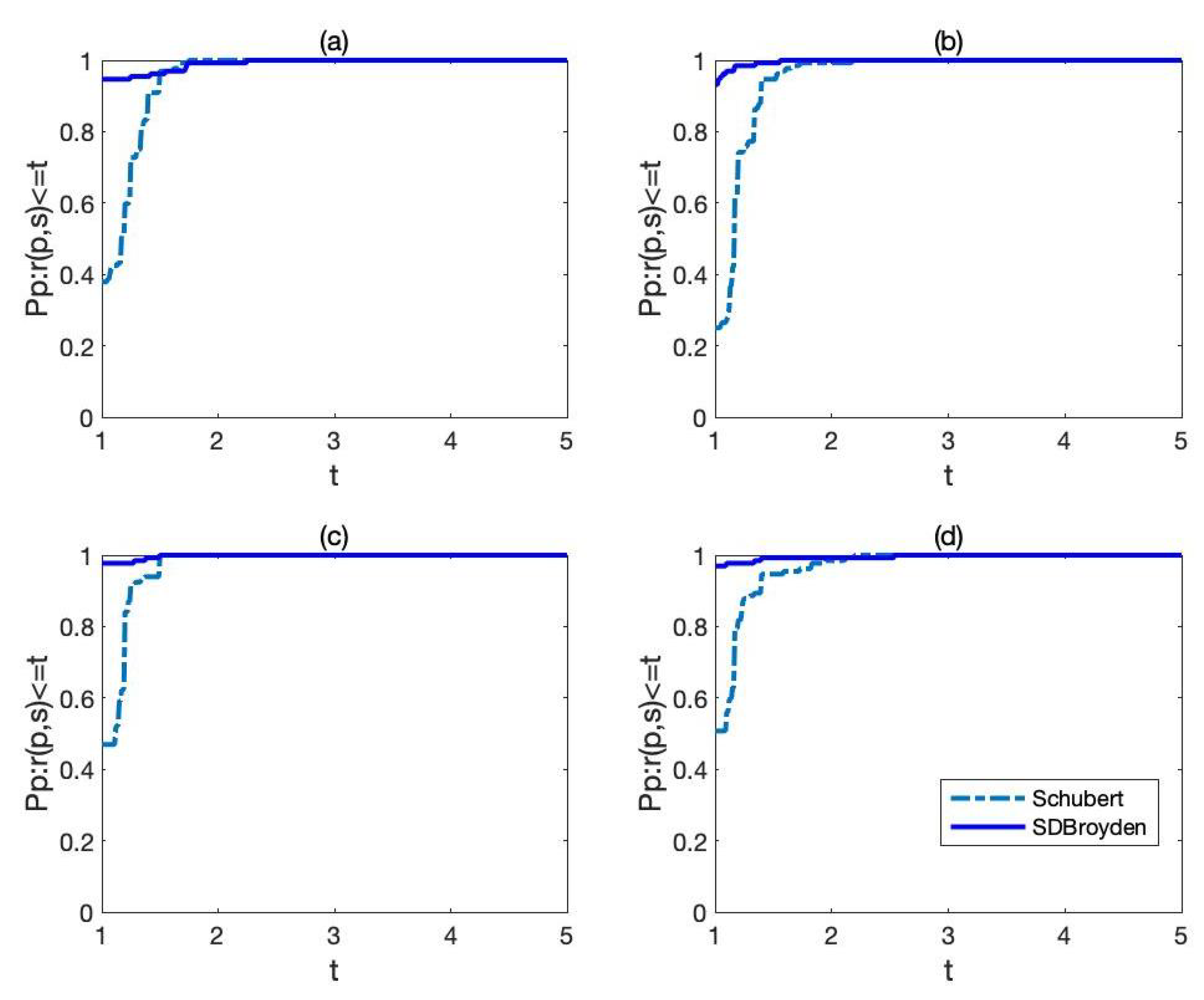
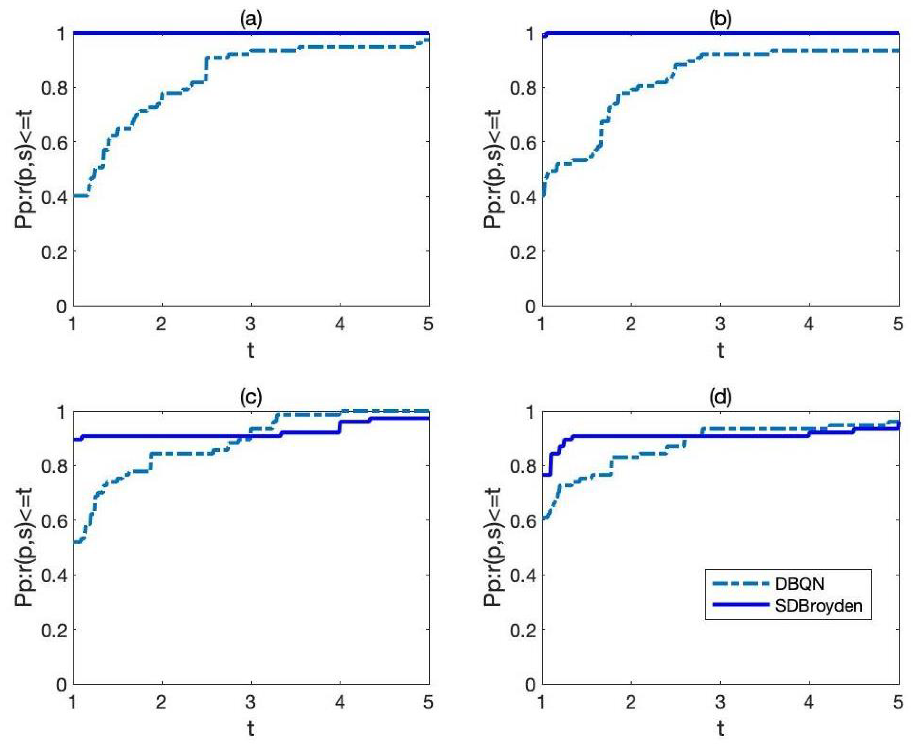
4. Numerical Experiments

In this section, we compare the SDBroyden method with Schubert’s method [8]. We also compare the SDBroyden method with a direct Broyden method and Newton’s method. All the methods are written in MATLAB R2018a and run in an iMac with 16G. The product $F^{\prime }\left(x\right)s$ is computed by the automatic differentiation tool TOLMAB [24].

The testing problems are listed in Appendix A. The Jacobian matrices of the tested problems have different structures such as: diagonal (Problem 1, 2), tridiagonal (Problems 3, 4, 5, 6, 7, 8), block-diagonal (Problems 9, 10, 11), and special structure (Problem 12). The parameters in Algorithm 1 are specified as [19]

$$ϵ={10}^{-5},\rho =0.9,{\sigma }_1={\sigma }_2=0.001,\beta =0.45,{\eta }_k=\frac{1}{{(k+1)}^2}.$$

For all the methods, we also stop the iteration if the number of iterations exceeds 200. We report the numerical performance of the above four methods in

Table 1. Results of Schubert’s method with $B_0=I$.

Pro(Dim)	10	100	1000	2000	10,000	20,000	50,000
(1)Ite	6	6	6	6	6	6	6
(1)Nfun	7	7	7	7	7	7	7
(1)R	0.8915	1.1098	1.1326	1.1338	1.1349	1.1350	1.1351
(1)Time(s)	0.0600	0.0000	0.0200	0.0000	0.0400	0.0400	0.0800
(2)Ite	7	7	7	7	7	7	7
(2)Nfun	8	8	8	8	8	8	8
(2)R	1.0407	1.0831	1.0919	1.0924	1.0929	1.0929	1.0929
(2)Time(s)	0.0100	0.0000	0.0100	0.0000	0.0200	0.0400	0.0900
(4)Ite	12	12	12	13	16	14	14
(4)Nfun	20	20	21	23	26	21	22
(4)R	0.3429	0.3440	0.3496	0.3441	0.3215	0.4183	0.4178
(4)Time(s)	0.0100	0.0000	0.0000	0.0100	0.1300	0.2400	0.4100
(5)Ite	20	17	25	22	22	16	21
(5)Nfun	63	32	64	73	40	36	48
(5)R	0.1051	0.2288	0.1106	0.1052	0.1902	0.2461	0.1664
(5)Time(s)	0.0400	0.0000	0.0000	0.0000	0.1400	0.1600	0.3400
(6)Ite	4	3	2	2	2	2	1
(6)Nfun	5	4	3	3	3	3	2
(6)R	1.5553	2.5624	3.0388	3.4398	4.3713	4.7641	3.8427
(6)Time(s)	0.0600	0.0000	0.0100	0.0000	0.0200	0.0300	0.0300
(7)Ite	10	8	6	6	4	4	3
(7)Nfun	11	11	8	8	6	6	5
(7)R	0.4980	0.3935	0.5299	0.5489	0.5362	0.5613	0.5820
(7)Time(s)	0.0300	0.0000	0.0000	0.0000	0.0300	0.0700	0.1100
(9)Ite	4	4	4	4	4	4	4
(9)Nfun	7	7	7	7	7	7	7
(9)R	Inf	Inf	Inf	Inf	Inf	Inf	Inf
(9)Time(s)	0.0400	0.0000	0.0000	0.0000	0.5100	0.9400	1.5100
Dim	12	102	1002	2001	10,002	20,001	50,001
(10)Ite	4	4	5	5	5	5	5
(10)Nfun	6	6	7	7	7	7	7
(10)R	1.0563	1.0563	1.5586	1.5586	1.5586	1.5586	1.5586
(10)Time(s)	0.0100	0.0000	0.1100	0.1300	0.2600	0.4500	0.8000
Dim	12	102	1002	2001	10,002	20,001	50,001
(11)Ite	6	6	7	7	7	7	7
(11)Nfun	8	8	9	9	9	9	9
(11)R	0.9175	0.9175	1.4972	1.4972	1.4972	1.4972	1.4972
(11)Time(s)	0.0300	0.0100	0.3000	0.1000	0.5200	0.7900	1.7100
(12)Ite	5	5	5	5	5	6	6
(12)Nfun	6	6	6	6	6	7	7
(12)R	1.1312	1.1156	1.1142	1.1142	1.1141	1.5918	1.5985
(12)Time(s)	0.0400	0.0000	0.0000	0.0000	0.0200	0.0500	0.1200

,

Table 2. Results of the SDBroyden method with $B_0=I$.

Pro(Dim)	10	100	1000	2000	10,000	20,000	50,000
(1)Ite	5	4	5	5	5	5	5
(1)Nfun	6	5	6	6	6	6	6
(1)R	1.6865	1.2113	2.1390	2.1415	2.1435	2.1437	2.1439
(1)Time(s)	0.0700	0.3600	1.4700	2.5200	13.2600	27.9500	88.0700
(2)Ite	5	5	5	5	5	6	6
(2)Nfun	6	6	6	6	6	7	7
(2)R	1.1023	1.1587	1.1705	1.1712	1.1718	1.9449	1.9450
(2)Time(s)	0.0300	0.2200	0.7800	1.7400	7.8200	20.2500	59.1100
(4)Ite	12	12	12	12	13	13	13
(4)Nfun	17	18	18	20	19	19	20
(4)R	0.4108	0.4253	0.4335	0.4085	0.4443	0.4747	0.4364
(4)Time(s)	0.2850	1.2600	11.2800	22.5000	139.3500	299.0400	834.3150
(5)Ite	16	16	20	18	19	20
(5)Nfun	29	35	57	48	52	48	56
(5)R	0.2179	0.2396	0.1505	0.1674	0.1738	0.1664	0.1675
(5)Time(s)	0.1400	0.5100	4.6200	17.5600	80.7900	182.6200	375.0000
(6)Ite	3	2	2	2	2	2	1
(6)Nfun	4	3	3	3	3	3	2
(6)R	1.4566	2.4834	4.4685	5.0549	5.6778	5.1461	3.8427
(6)Time(s)	0.0500	0.0800	0.6200	1.1100	6.5800	13.2100	20.2600
(7)Ite	10	8	6	6	4	4	3
(7)Nfun	11	11	8	8	6	6	5
(7)R	0.4980	0.3935	0.5299	0.5489	0.5362	0.5613	0.5820
(7)Time(s)	0.1700	0.3800	2.0700	4.1000	14.1400	29.3900	69.4400
(9)Ite	4	4	4	4	4	4	4
(9)Nfun	6	6	6	6	6	6	6
(9)R	Inf	Inf	Inf	Inf	Inf	Inf	Inf
(9)Time(s)	0.0500	0.1450	0.5600	1.3000	13.6700	28.0700	84.4600
Dim	12	102	1002	2001	10,002	20,001	50,001
(10)Ite	3	3	3	3	4	4	4
(10)Nfun	5	5	5	5	6	6	6
(10)R	1.3420	1.3420	1.3420	1.3420	2.3852	2.3852	2.3852
(10)Time(s)	0.0600	0.1700	0.9000	1.8100	10.8000	21.5800	64.8000
Dim	12	102	1002	2001	10,002	20,001	50,001
(11)Ite	5	6	6	6	6	6	6
(11)Nfun	7	8	8	8	8	8	8
(11)R	1.0013	1.8209	1.8209	1.8209	1.8209	1.8209	1.8209
(11)Time(s)	0.0900	0.3000	2.1500	3.5300	18.8500	40.5600	109.5900
(12)Ite	4	4	4	4	4	4	4
(12)Nfun	5	5	5	5	5	5	5
(12)R	1.7679	1.7551	1.7540	1.7539	1.7538	1.7538	1.7538
(12)Time(s)	0.0500	0.1500	0.6700	1.2700	6.4500	13.7700	43.1500

,

Table 3. Results of Schubert’s method with $B_0=F^{\prime }\left(x_0\right)$.

Pro(Dim)	10	100	1000	2000	10,000	20,000	50,000
(1)Ite	6	6	6	6	6	6	6
(1)Nfun	8	7	7	7	8	8	8
(1)R	0.8661	0.9523	0.9693	0.9703	0.9077	0.9077	0.9077
(1)Time(s)	0.0000	0.0000	0.0100	0.0000	0.0300	0.0400	0.0900
(2)Ite	6	6	6	6	6	6	6
(2)Nfun	7	7	7	7	7	7	7
(2)R	1.1690	1.1982	1.2024	1.2026	1.2028	1.2028	1.2028
(2)Time(s)	0.0500	0.0000	0.0000	0.0000	0.0400	0.0400	0.0800
(3)Ite	10	11	11	11	11	11	11
(3)Nfun	11	12	12	12	12	12	12
(3)R	0.6216	0.5988	0.6391	0.6515	0.6806	0.6931	0.7097
(3)Time(s)	0.0400	0.0000	0.0200	0.0000	0.0900	0.1400	0.2000
(4)Ite	13	23	23	29	21	30	27
(4)Nfun	25	44	45	58	44	81	72
(4)R	0.2705	0.1743	0.1820	0.1455	0.2054	0.1256	0.2367
(4)Time(s)	0.0500	0.0000	0.0100	0.0000	0.0600	0.1100	0.1800
(5)Ite	18	24	26	24	23	23	23
(5)Nfun	26	44	68	54	42	42	42
(5)R	0.2543	0.1425	0.1190	0.1420	0.1864	0.1900	0.1947
(5)Time(s)	0.0600	0.0000	0.0000	0.0000	0.2100	0.2400	0.5100
(6)Ite	5	3	2	2	2	2	2
(6)Nfun	6	4	3	3	3	3	3
(6)R	1.1562	1.8540	2.4963	2.8469	3.6620	4.0131	4.4773
(6)Time(s)	0.0400	0.0000	0.0100	0.0000	0.0100	0.0400	0.0700
(7)Ite	12	12	7	4	1	1	1
(7)Nfun	18	21	11	6	2	2	2
(7)R	0.2585	0.2158	0.3382	0.6401	1.7302	1.8807	2.0797
(7)Time(s)	0.0100	0.0000	0.0100	0.0100	0.0100	0.0400	0.0500
(8)Ite	8	8	8	7	7	7	7
(8)Nfun	10	11	10	9	10	10	19
(8)R	0.5898	0.5317	0.5779	0.5637	0.5789	0.5881	0.6023
(8)Time(s)	0.0300	0.0000	0.0000	0.0000	0.4200	1.3500	3.8000
(9)Ite	3	3	3	3	3	3	3
(9)Nfun	4	4	4	4	4	4	4
(9)R	4.0327	4.0327	4.0327	4.0327	4.0327	4.0327	4.0327
(9)Time(s)	0.0000	0.0100	0.0000	0.0100	0.0400	0.0700	0.2300
Dim	12	102	1002	2001	10,002	20,001	50,001
(10)Ite	9	10	10	10	11	11	11
(10)Nfun	10	11	11	11	12	12	12
(10)R	0.5520	0.5886	0.5886	0.5886	0.6701	0.6701	0.6701
(10)Time(s)	0.0200	0.0200	0.2800	0.2600	0.7400	1.1800	2.4700
Dim	12	102	1002	2001	10,002	20,001	50,001
(11)Ite	5	6	6	6	6	6	6
(11)Nfun	6	7	7	7	7	7	7
(11)R	1.1416	1.7664	1.7664	1.7664	1.7664	1.7664	1.7664
(11)Time(s)	0.0300	0.0300	0.2000	0.2200	0.4300	0.6500	1.3500
(12)Ite	8	8	8	8	8	8	8
(12)Nfun	9	9	9	9	9	9	10
(12)R	0.5909	0.6449	0.7003	0.7170	0.7558	0.7725	0.7210
(12)Time(s)	0.0200	0.0000	0.0000	0.0100	0.0600	0.1100	0.1800

,

Table 4. Results of the SDBroyden method with $B_0=F^{\prime }\left(x_0\right)$.

Pro(Dim)	10	100	1000	2000	10,000	20,000	50,000
(1)Ite	4	5	5	5	5	5	5
(1)Nfun	6	6	6	6	7	7	7
(1)R	0.9211	1.6975	1.7287	1.7304	1.6431	1.6431	1.6431
(1)Time(s)	0.0300	0.2200	1.6600	2.6400	14.2100	29.4400	88.3100
(2)Ite	4	4	4	5	5	5	5
(2)Nfun	5	5	5	6	6	6	6
(2)R	1.2544	1.2872	1.2916	2.1183	2.1187	2.1187	2.1187
(2)Time(s)	0.0400	0.1300	0.6600	1.6900	7.7100	16.1100	48.0500
(3)Ite	11	11	11	11	11	11	11
(3)Nfun	12	12	12	12	12	12	12
(3)R	0.5609	0.5642	0.6045	0.6170	0.6460	0.6586	0.6751
(3)Time(s)	0.1900	0.6100	5.5200	10.8000	55.6500	112.3100	307.9200
(4)Ite	13	17	17	18	20	23	18
(4)Nfun	24	28	28	35	38	59	56
(4)R	0.2867	0.2688	0.2707	0.2218	0.6251	0.5620	0.6294
(4)Time(s)	0.1500	0.8900	5.8100	12.4900	66.7200	142.7600	402.8600
(5)Ite	23	21	22	20	20	20	20
(5)Nfun	46	40	35	34	34	34	34
(5)R	0.1996	0.1651	0.1957	0.2207	0.2309	0.2354	0.2412
(5)Time(s)	0.3500	1.7100	13.8200	26.4100	143.4000	293.5900	341.0000
(6)Ite	4	3	2	2	2	2	2
(6)Nfun	5	4	3	3	3	3	3
(6)R	1.1204	2.0735	2.4895	2.8401	3.6550	4.0062	4.4704
(6)Time(s)	0.1000	0.1800	1.1100	1.6500	8.7100	20.2800	53.0700
(7)Ite	12	12	7	4	1	1	1
(7)Nfun	18	21	11	6	2	2	2
(7)R	0.2585	0.2158	0.3382	0.6401	1.7302	1.8807	2.0797
(7)Time(s)	0.2100	0.8900	3.9500	4.4100	5.9700	12.5000	32.9300
(8)Ite	11	7	6	6	6	6	6
(8)Nfun	14	9	8	8	9	9	9
(8)R	0.4237	0.5767	0.6337	0.8068	0.7790	0.7811	0.7995
(8)Time(s)	0.1900	0.4100	2.8100	6.1500	13.3900	24.0600	48.4500
(9)Ite	3	3	3	3	3	3	3
(9)Nfun	4	4	4	4	4	4	4
(9)R	Inf	Inf	Inf	Inf	Inf	Inf	Inf
(9)Time(s)	0.0300	0.1400	0.5400	1.3100	5.7400	13.2200	37.1600
Dim	12	102	1002	2001	10,002	20,001	50,001
(10)Ite	8	9	9	9	9	9	9
(10)Nfun	10	11	11	11	11	11	11
(10)R	0.5616	0.6068	0.6068	0.6068	0.6309	0.6374	0.6438
(10)Time(s)	0.1300	0.4600	3.5500	6.6100	39.4200	82.5100	242.4400
Dim	12	102	1002	2001	10,002	20,001	50,001
(11)Ite	4	5	5	5	5	5	5
(11)Nfun	5	6	6	6	6	6	6
(11)R	1.3736	2.3204	2.3204	2.3204	2.3204	2.3204	2.3204
(11)Time(s)	0.0600	0.2300	1.8600	2.9500	15.8600	33.6900	92.8300
(12)Ite	8	8	8	8	8	8	7
(12)Nfun	9	9	9	9	9	9	9
(12)R	0.6704	0.7239	0.7793	0.7960	0.8348	0.8515	0.7721
(12)Time(s)	0.1100	0.2900	2.1600	3.7500	19.3700	41.5900	106.5800

,

Table 5. Results of the DBQN method with $B_0=I$.

Pro(Dim)	10	20	50	100	200	500	1000
(1)Ite	5	4	4	4	4	5	5
(1)Nfun	6	5	5	5	5	6	6
(1)R	1.6865	1.0998	1.1828	1.2113	1.2258	2.1341	2.1390
(1)Time(s)	0.2900	0.1900	0.1500	0.5400	0.5600	3.1000	19.3500
(2)Ite	5	5	5	5	5	6	6
(2)Nfun	6	6	6	6	6	7	7
(2)R	0.9943	1.0107	1.0229	1.0274	1.0297	1.2624	1.2631
(2)Time(s)	0.1000	0.1300	0.1600	0.2100	0.4500	3.1700	21.8400
(4)Ite	24	33	53	59	58	73	95
(4)Nfun	42	68	117	118	120	187	318
(4)R	0.1630	0.0963	0.0606	0.0585	0.0587	0.0383	0.0233
(4)Time(s)	1.0800	1.9000	6.3600	12.6900	24.1200	97.9500	510.2200
(6)Ite	6	5	3	3	2	2	2
(6)Nfun	7	6	4	4	3	3	3
(6)R	0.8516	1.1498	1.6230	2.0975	2.4436	3.0384	3.4893
(6)Time(s)	0.2000	0.2700	0.1500	0.7800	0.4200	1.5500	8.1900
(7)Ite	15	23	20	24	14	12	11
(7)Nfun	22	32	30	27	29	22	20
(7)R	0.2285	0.1356	0.1421	0.1510	0.1401	0.1741	0.1863
(7)Time(s)	0.5700	0.6900	1.3200	3.0500	3.9500	10.9700	47.1200
Dim	12	21	51	102	201	501	1002
(10)Ite	3	3	3	3	3	3	3
(10)Nfun	5	5	5	5	5	5	5
(10)R	1.3420	1.3420	1.3420	1.3420	1.3420	1.3420	1.3420
(10)Time(s)	0.1500	0.1800	0.1300	0.2600	0.6400	2.0000	10.9100
Dim	12	21	51	102	201	501	1002
(11)Ite	7	7	7	7	8	8	8
(11)Nfun	13	13	13	13	14	14	14
(11)R	0.5532	0.5532	0.5532	0.5532	0.6535	0.6224	0.5851
(11)Time(s)	0.2200	0.3400	0.2800	0.5700	1.3100	4.8700	33.8700
(12)Ite	4	4	4	4	4	4	4
(12)Nfun	5	5	5	5	5	5	5
(12)R	1.9415	1.8389	1.7860	1.7696	1.7617	1.7569	1.7554
(12)Time(s)	0.1400	0.1700	0.1500	0.2500	0.5000	2.1700	13.6100

,

Table 6. Results of the DBQN method with $B_0=F^{\prime }\left(x_0\right)$.

Pro(Dim)	10	20	50	100	200	500	1000
(1)Ite	4	5	5	5	5	5	5
(1)Nfun	6	6	6	6	6	6	6
(1)R	0.9211	1.5530	1.6623	1.6975	1.7149	1.7252	1.7287
(1)Time(s)	0.0900	0.2200	0.4800	0.5100	0.6700	3.1600	20.2400
(2)Ite	11	11	12	12	12	13	13
(2)Nfun	12	12	13	13	13	14	14
(2)R	0.4726	0.4677	0.4819	0.4822	0.4827	0.4807	0.4808
(2)Time(s)	0.2000	0.3300	0.3200	0.5100	1.1300	6.7900	47.0600
(3)Ite	10	11	11	11	11	11	11
(3)Nfun	11	12	12	12	12	12	12
(3)R	0.5629	0.5496	0.5542	0.5641	0.5754	0.5912	0.6035
(3)Time(s)	0.4800	0.6900	0.7200	1.1800	2.2700	9.2200	45.4800
(4)Ite	16	25	32	29	35	34	33
(4)Nfun	23	40	56	58	64	83	67
(4)R	0.3164	0.1641	0.1241	0.1219	0.1142	0.0897	0.1128
(4)Time(s)	0.7800	1.2400	4.0200	6.7600	15.7000	49.1800	180.5200
(6)Ite	5	5	4	4	3	3	3
(6)Nfun	6	6	5	5	4	4	4
(6)R	1.0196	1.1784	1.5102	1.9224	1.8193	2.2563	2.5914
(5)Time(s)	0.1000	0.1700	0.3200	0.4400	0.6200	2.2700	12.2300
(7)Ite	3	3	3	3	3	1	1
(7)Nfun	4	4	4	4	4	2	2
(7)R	1.5674	1.8740	2.2760	2.5987	2.9294	2.0320	2.2588
(7)Time(s)	0.1100	0.1000	0.3100	0.3900	0.7100	0.8600	4.2900
(8)Ite	14	14	18	23	20	23	24
(8)Nfun	20	23	38	59	44	76	80
(8)R	0.2827	0.2437	0.1454	0.0953	0.1199	0.0731	0.0670
(8)Time(s)	0.6300	1.0300	1.6100	2.7100	5.0500	20.8500	102.1800
Dim	12	21	51	102	201	501	1002
(9)Ite	3	3	3	3	3	3	3
(9)Nfun	4	4	4	4	4	4	4
(9)R	3.8134	3.7605	3.7383	3.5184	3.4381	3.6076	3.5910
(9)Time(s)	0.0300	0.0600	0.2200	0.2200	0.3700	1.4300	9.5300
Dim	12	21	51	102	201	501	1002
(10)Ite	9	9	9	9	9	9	9
(10)Nfun	10	10	10	10	10	10	10
(10)R	0.7420	0.7420	0.7420	0.7420	0.7420	0.7420	0.7420
(10)Time(s)	0.3200	0.2500	0.4300	1.4000	1.6200	6.0500	32.8000
Dim	12	21	51	102	201	501	1002
(11)Ite	5	5	5	5	5	5	5
(11)Nfun	6	6	6	6	6	6	6
(11)R	1.3488	1.3488	1.3488	1.3488	1.3488	1.3488	1.3488
(11)Time(s)	0.1300	0.1300	0.1900	0.4200	0.7500	3.0700	20.7800
(12)Ite	11	13	15	15	15	15	15
(12)Nfun	12	14	16	16	16	16	16
(12)R	0.4607	0.3912	0.3475	0.3534	0.3610	0.3720	0.3808
(12)Time(s)	0.1500	0.3900	0.5600	0.9900	1.9300	8.0200	55.5800

and

Table 7. Results of the Newton’s method.

Pro(Dim)	10	20	50	100	200	500	1000
(1)Ite	4	5	5	5	5	5	5
(1)Nfun	6	6	6	6	6	6	6
(1)R	0.9211	1.5530	1.6623	1.6975	1.7149	1.7252	1.7287
(1)Time(s)	0.0000	0.0000	0.0100	0.0700	0.1900	1.9100	16.8700
(2)Ite	4	4	4	4	4	4	4
(2)Nfun	5	5	5	5	5	5	5
(2)R	1.2544	1.2704	1.2826	1.2872	1.2896	1.2911	1.2916
(2)Time(s)	0.0100	0.0000	0.0100	0.0100	0.1500	2.2600	13.3200
(3)Ite	4	4	4	4	4	4	5
(3)Nfun	5	5	5	5	5	5	6
(3)R	1.2884	1.3061	1.3333	1.3542	1.3729	1.3913	2.2609
(3)Time(s)	0.0000	0.0000	0.0100	0.0100	0.1900	2.1300	17.8300
(4)Ite	16	17	18	18	19	19	20
(4)Nfun	17	18	19	19	20	20	21
(4)R	0.3721	0.3649	0.3625	0.3617	0.3620	0.3618	0.3623
(4)Time(s)	0.0200	0.0100	0.0100	0.1100	0.8500	7.8600	67.7600
(6)Ite	15	12	8	6	5	4	3
(6)Nfun	16	13	9	7	6	5	4
(6)R	0.3600	0.4488	0.6793	0.9078	1.1567	1.4961	1.7423
(6)Time(s)	0.0300	0.0000	0.0100	0.0600	0.2000	1.4900	9.9400
(7)Ite	22	18	12	8	4	1	1
(7)Nfun	23	19	13	9	5	2	2
(7)R	0.1919	0.2323	0.3217	0.4503	0.7825	2.0320	2.2588
(7)Time(s)	0.0300	0.0000	0.0200	0.0600	0.1200	0.3800	3.3100
(9)Ite	2	2	2	2	2	2	2
(9)Nfun	3	3	3	3	3	3	3
(9)R	Inf	Inf	Inf	Inf	Inf	Inf	Inf
(9)Time(s)	0.0000	0.0000	0.0100	0.0100	0.1000	0.7000	5.8800
Dim	12	21	51	102	201	501	1002
(11)Ite	3	3	3	3	3	3	3
(11)Nfun	4	4	4	4	4	4	4
(11)R	2.0137	2.0137	2.0137	2.0137	2.0137	2.0137	2.0137
(11)Time(s)	0.0100	0.0000	0.0100	0.0200	0.1100	1.0600	11.1200
(12)Ite	4	4	4	4	4	4	4
(12)Nfun	5	5	5	5	5	5	5
(12)R	1.4972	1.4718	1.4581	1.4541	1.4523	1.4511	1.4508
(12)Time(s)	0.0100	0.0000	0.0100	0.0300	0.1600	1.2900	12.0100

and Figure 1 and Figure 2, where the meaning of each column is as follows:

Schubert:	Schubert’s method;
SDBroyden:	sparse direct Broyden method with LF condition;
Pro	the number of the test problem;
Dim:	the dimension of the problem;
Ite	the total number of iterations;
Nfun:	the total number of function evaluations;
R:	Broyden’s mean convergence rate;
Time(s):	CPU time in second;
Fail:	the stopping criterion was not satisfied.

(1) In the first set of our numerical experiments, we test the performance of the SDBroyden method and Schubert’s method. When $B_0$ is chosen as unit matrix I, the results are listed in Table 1 and Table 2, respectively. For SDBroyden method and Schubert’s method, we compute the problems with dimensions ($n=$ 10, 20, 50, 100, 200, 500, 1000, 2000, 5000, 10,000, 20,000, 50,000), but we select a subset of the dimensions ($n=$ 10, 100, 1000, 2000, 10,000, 20,000, 50,000) to improve the readability of the corresponding tables. The two methods fail on two problems (3, 8). Considering the iteration counts, the SDBroyden method is more efficient than Schubert’s method on seven problems (1, 2, 4, 5, 10, 11, 12), equivalent to Schubert’s method on three problems (6, 7, 9). For the total number of function evaluations, the SDBroyden method has better performance on seven problems (1, 2, 4, 9, 10, 11, 12), while Schubert’s method needs less function evaluations on one problem (5), and both methods are equivalent on two problems (6, 7). As for the Broyden’s mean convergence rate, SDBroyden works well on seven problems (1, 2, 4, 6, 10, 11, 12), equal to Schubert’s method on three problems (5, 7, 9). It can be seen that the SDBroyden method outperforms Schubert’s method in iteration counts, function evaluation counts, and Broyden’s mean convergence rate.

When $B_0$ is chosen as the exact Jacobian matrix $F^{\prime }\left(x_0\right)$, the results are given in Table 3 and Table 4, respectively. The two methods solve the 12 problems successfully. The SDBroyden method needs fewer iterations than Schubert’s method on seven problems (1, 2, 4, 5, 8, 10, 11), equal iterations with Schubert’s method on five problems (3, 6, 7, 9, 12). For the total number of function evaluations, the SDBroyden method is more efficient than Schubert’s method on six problems (1, 2, 4, 5, 8, 11) and equivalent to Schubert’s method on six problems (3, 6, 7, 9, 10, 12). As for the Broyden’s mean convergence rate, SDBroyden has better performance on nine problems (1, 2, 3, 4, 5, 8, 10, 11, 12) and equals Schubert’s method on two problems (7, 9). The two methods are competitive on one problem (6). It also can be seen that the SDBroyden method outperforms Schubert’s method in terms of number of iterations, number of function evaluations, and Broyden’s mean convergence rate. Meanwhile, the CPU time of SDBroyden method is mostly more than that of Schubert’s method.

Performance ration [25] is used to compare the numerical performance. For given solvers set S and problems set P, let $t_{p,s}$ be the number of iterations, the number of function evaluations or others, required to solve problem p by solver s. Then, define the performance ration as

$$r_{p,s}=\frac{t_{p,s}}{min\{t_{p,q}:q\in S\}},$$

whose distribution function is defined as

$${\rho }_s\left(t\right)=\frac{1}{N_p}\mathrm{size}\{p\in P:r_{p,s}\le t\},$$

where $N_p$ is the number of problems in the set P. Thus, ${\rho }_s:R\to [0,1]$ was the probability for solver $s\in S$ that a performance ratio $r_{p,s}$ was within a factor $t\in R$ of the best possible ratio. According to the definition of performance profiles, we can see that the top curve corresponds to the best solver.

In Figure 1, the performance of the two methods: the SDBroyden method and Schubert’s method, relative to the number of iterations, and the number of function evaluations are evaluated. Figure 1 indicates that SDBroyden has better performance than Schubert’s method on the number of iterations and number of function evaluations.

(2) In the second set of numerical experiments, we compare the SDBroyden method with the direct Broyden quasi-Newton method (DBQN). We give the results of the DBQN method with $B_0=I$ in Table 5. The DBQN method fails on four problems (3, 5, 8, 9). For the number of iterations and number of function evaluations, the SDBroyden method needs less iterations on five problems (2, 4, 6, 7, 11) and equals DBQN on three problems (1, 10, 12). For the Broyden’s mean convergence rate, the SDBroyden method performs better on five problems (2, 4, 6, 7, 11), equals DBQN on two problems (1, 10), and works badly on one problem (12).

The results of the DBQN method with $B_0=F^{\prime }\left(x_0\right)$ are listed in Table 6. The DBQN method fails on one problem (5). For the number of iterations, SDBroyden is better than the DBQN method on seven problems (2, 4, 6, 8, 10, 11, 12), equivalent to the DBQN method on three problems (1, 3, 9). At the same time, DBQN performs well on one problem (7). For the number of function evaluations and Broyden’s mean convergence rate, SDBroyden is excellent on six problems (2, 4, 6, 8, 11, 12), while the DBQN method works well on one problem (10). The two methods coincide with each other on three problems (3, 9, 10).

In Figure 2, we also give the comparison of the SDBroyden method and DBQN method relative to the number of iterations and number of function evaluations. It can be seen that the top curve corresponds to the SDBroyden method. This means that the SDBroyden method has satisfactory performance in terms of number of iterations and number of function evaluations when compared with its dense version.

(3) In the third set of our numerical experiments, we compare the SDBroyden method with Newton’s method, where the results are listed in Table 7. Newton’s method fails on three problems (5, 8, 10). One can see that the SDBroyden method requires slightly more iterations than Newton’s method in most tests and has no significant advantages in the number of iterations, number of function evaluations, and Broyden’s mean convergence rate. However, the CPU time for Newton’s method is much higher than that of the SDBroyden method. Moreover, the CPU time of Newton’s method increases significantly faster than that of the quasi-Newton methods. Thus, the SDBroyden method can be applied to solve large-scale nonlinear equations.

5. Conclusions

We have developed a sparse direct Broyden quasi-Newton method for solving large-scale nonlinear equations, which is the sparse case of the direct Broyden method and is an extension of Broyden’s method. The method approximates the Jacobian matrix by least change updating and satisfies the sparsity condition and direct tangent condition simultaneously. We show that the method is locally and superlinearly convergent. Combined with a nonmonotone line search, we also establish the global and superlinear convergence. In particular, the unit step length is essentially accepted. Our numerical results show that the proposed method is effective and competitive for sparse nonlinear equations.

References

1. Yuan, Y.X. Recent advances in numerical methods for nonlinear equations and nonlinear least squares. Numer. Algebra Control Optim. 2011, 1, 15–34. [Google Scholar] [CrossRef]
2. Sun, W.; Yuan, Y.X. Optimization Theory and Methods: Nonlinear Programming; Springer Science & Business Media: New York, NY, USA, 2006. [Google Scholar]
3. Wright, S.; Nocedal, J. Numerical Optimization; Springer Science: New York, NY, USA, 1999; Volume 35, p. 7. [Google Scholar]
4. Fletcher, R. Practical Methods of Optimization; John Wiley & Sons: Hoboken, NJ, USA, 2013. [Google Scholar]
5. Broyden, C.G. A class of methods for solving nonlinear simultaneous equations. Math. Comput. 1965, 19, 577–593. [Google Scholar] [CrossRef]
6. Broyden, C.G.; Dennis, J.E., Jr.; Moré, J.J. On the local and superlinear convergence of quasi-Newton methods. IMA J. Appl. Math. 1973, 12, 223–245. [Google Scholar] [CrossRef]
7. Dennis, J.E.; Moré, J.J. Quasi–Newton methods, motivation and theory. SIAM Rev. 1977, 19, 46–89. [Google Scholar] [CrossRef] [Green Version]
8. Schubert, L.K. Modification of a quasi-Newton method for nonlinear equations with a sparse Jacobian. Math. Comput. 1970, 24, 27–30. [Google Scholar] [CrossRef]
9. Toint, P.L. On sparse and symmetric matrix updating subject to a linear equation. Math. Comput. 1977, 31, 954–961. [Google Scholar] [CrossRef]
10. Nocedal, J. Updating quasi-Newton matrices with limited storage. Math. Comput. 1980, 35, 773–782. [Google Scholar] [CrossRef]
11. Van de Rotten, B.; Lunel, S.V. A limited memory Broyden method to solve high-dimensional systems of nonlinear equations. In Proceedings of the International Conference on Differential Equations, Hasselt, Belgium, 22–26 July 2003; pp. 196–201. [Google Scholar]
12. Griewank, A.; Toint, P.L. Partitioned variable metric updates for large structured optimization problems. Numer. Math. 1982, 39, 119–137. [Google Scholar] [CrossRef]
13. Griewank, A.; Toint, P.L. Local convergence analysis for partitioned quasi-Newton updates. Numer. Math. 1982, 39, 429–448. [Google Scholar]
14. Cao, H.P.; Li, D.H. Partitioned quasi-Newton methods for sparse nonlinear equations. Comput. Optim. Appl. 2017, 66, 481–505. [Google Scholar] [CrossRef]
15. Leong, W.J.; Hassan, M.A.; Yusuf, M.W. A matrix-free quasi-Newton method for solving large-scale nonlinear systems. Comput. Math. Appl. 2011, 62, 2354–2363. [Google Scholar] [CrossRef] [Green Version]
16. Li, D.H.; Wang, X.; Huang, J. Diagonal BFGS updates and applications to the limited memory BFGS method. Comput. Optim. Appl. 2022, 81, 829–856. [Google Scholar] [CrossRef]
17. Martínez, J.M. A quasi-Newton method with modification of one column per iteration. Computing 1984, 33, 353–362. [Google Scholar] [CrossRef]
18. Griewank, A. The “global” convergence of Broyden-like methods with suitable line search. ANZIAM J. 1986, 28, 75–92. [Google Scholar] [CrossRef] [Green Version]
19. Li, D.H.; Fukushima, M. A derivative-free line search and global convergence of Broyden-like method for nonlinear equations. Optim. Methods Softw. 2000, 13, 181–201. [Google Scholar] [CrossRef]
20. Griewank, A.; Walther, A. On constrained optimization by adjoint based quasi-Newton methods. Optim. Methods Softw. 2002, 17, 869–889. [Google Scholar] [CrossRef]
21. Schlenkrich, S.; Griewank, A.; Walther, A. On the local convergence of adjoint Broyden methods. Math. Program. 2010, 121, 221–247. [Google Scholar] [CrossRef]
22. Marwil, E. Convergence results for Schubert’s method for solving sparse nonlinear equations. SIAM J. Numer. Anal. 1979, 16, 588–604. [Google Scholar] [CrossRef]
23. Powell, M.J.D. A hybrid method for nonlinear equations. In Numerical Methods for Nonlinear Algebraic Equations; Gordon and Breach: London, UK, 1970. [Google Scholar]
24. Forth, S.A.; Edvall, M.M. User Guide for MAD-MATLAB Automatic Differentiation Toolbox TOMLAB/MAD; Version 1.1 The Forward Mode; TOMLAB Optimisation Inc.: San Diego, CA, USA, 2007; p. 92101. [Google Scholar]
25. Dolan, E.D.; Moré, J.J. Benchmarking optimization software with performance profiles. Math. Program. 2002, 91, 201–213. [Google Scholar] [CrossRef]
26. La Cruz, W.; Martínez, J.; Raydan, M. Spectral residual method without gradient information for solving large-scale nonlinear systems of equations. Math. Comput. 2006, 75, 1429–1448. [Google Scholar] [CrossRef] [Green Version]
27. Raydan, M. The Barzilai and Borwein gradient method for the large scale unconstrained minimization problem. SIAM J. Numer. Anal. 1997, 7, 26–33. [Google Scholar] [CrossRef]
28. Gomes-Ruggiero, M.A.; Martínez, J.M.; Moretti, A.C. Comparing algorithms for solving sparse nonlinear systems of equations. SIAM J. Sci. Comput. 1992, 13, 459–483. [Google Scholar] [CrossRef]
29. Li, G. Successive column correction algorithms for solving sparse nonlinear systems of equations. Math. Program. 1989, 43, 187–207. [Google Scholar] [CrossRef] [Green Version]
30. Bing, Y.; Lin, G. An efficient implementation of Merrill’s method for sparse or partially separable systems of nonlinear equations. SIAM J. Optim. 1991, 1, 206–221. [Google Scholar] [CrossRef]
31. Moré, J.J.; Garbow, B.S.; Hillstrom, K.E. Testing unconstrained optimization software. ACM Trans. Math. Softw. (TOMS) 1981, 7, 17–41. [Google Scholar] [CrossRef]
32. Roberts, S.M.; Shipman, J.S. On the closed form solution of Troesch’s problem. J. Comput. Phys. 1976, 21, 291–304. [Google Scholar] [CrossRef]
33. Gasparo, M.G. A nonmonotone hybrid method for nonlinear systems. Optim. Methods Softw. 2000, 13, 79–94. [Google Scholar] [CrossRef]
34. Friedlander, A.; Gomes-Ruggiero, M.A.; Kozakevich, D.N.; Mario Martínez, J.; Augusta Santos, S. Solving nonlinear systems of equations by means of quasi-neston methods with a nonmonotone stratgy. Optim. Methods Softw. 1997, 8, 25–51. [Google Scholar] [CrossRef]
35. Luksan, L.; Matonoha, C.; Vlcek, J. Problems for Nonlinear Least Squares and Nonlinear Equations; Technical Report 1259; Institute of Computer Science, Academy of Sciences of the Czech Republic: Prague, Czech Republic, 2018. [Google Scholar]
Figure 1. Performance profiles for SDBroyden and Schubert: (a) results comparison on the number of iterations with B 0 = I ; (b) results comparison on the number of function evaluations with B 0 = I ; (c) results comparison on the number of iterations with B 0 = F ( x 0 ) ; (d) results comparison on the number of function evaluations with B 0 = F ( x 0 ) .
Symmetry 14 01552 g001
Figure 2. Performance profiles of SDBroyden and DBQN (a) results comparison on the number of iterations with B 0 = I ; (b) results comparison on the number of function evaluations with B 0 = I ; (c) results comparison on the number of iterations with B 0 = F ( x 0 ) ; (d) results comparison on the number of function evaluations with B 0 = F ( x 0 ) .
Symmetry 14 01552 g002