The Stability of a Hydrodynamic Bravais Lattice

Abstract

We present the results of a theoretical investigation of the stability and collective vibrations of a two-dimensional hydrodynamic lattice comprised of millimetric droplets bouncing on the surface of a vibrating liquid bath. We derive the linearized equations of motion describing the dynamics of a generic Bravais lattice, as encompasses all possible tilings of parallelograms in an infinite plane-filling array. Focusing on square and triangular lattice geometries, we demonstrate that for relatively low driving accelerations of the bath, only a subset of inter-drop spacings exist for which stable lattices may be achieved. The range of stable spacings is prescribed by the structure of the underlying wavefield. As the driving acceleration is increased progressively, the initially stationary lattices destabilize into coherent oscillatory motion. Our analysis yields both the instability threshold and the wavevector and polarization of the most unstable vibrational mode. The non-Markovian nature of the droplet dynamics renders the stability analysis of the hydrodynamic lattice more rich and subtle than that of its solid state counterpart.

1. Introduction

The collective vibrations of atoms within a crystal lattice, referred to as phonons, are of fundamental interest in materials science and solid-state physics, and govern bulk properties of the crystal such as the heat capacity, thermal and electrical conductivity, and elastic modulus [1,2,3,4]. Complementary insight into lattice dynamics is often gained through consideration of macroscopic analog systems, including mass-and-spring networks [5,6] and more complex metamaterials [7,8]. Numerous hydrodynamic analogues of crystals have been explored, from Bragg’s packed bubbles at an air–liquid interface [9] to more recent studies of vibrations in lattices of colloidal particles [10,11,12,13,14] and microfluidic droplets [15,16,17,18]. We here consider theoretically the dynamics of a two-dimensional lattice comprised of millimetric droplets that bounce on the surface of a vibrating liquid bath and are coupled through an underlying Faraday wavefield.

A fluid bath vibrating vertically with acceleration $\gamma sin\left(2\pi ft\right)$ will destabilize into a subharmonic field of standing Faraday waves, characterized by period $T_F=2/f$ and wavelength ${\lambda }_F$ (as is related to ${\omega }_F=\pi f$ through the standard water-wave dispersion relation), when the vibrational acceleration $\gamma$ exceeds a critical value ${\gamma }_F$ known as the Faraday threshold [19,20]. Below ${\gamma }_F$, but above the bouncing threshold ${\gamma }_B<{\gamma }_F$, a millimetric droplet may bounce indefinitely on the bath’s surface, generating a spatially extended, temporally decaying wavefield at each impact [21,22]. As $\gamma$ is gradually increased beyond ${\gamma }_B$, the droplet’s bouncing period increases until eventually becoming twice that of the vibrational driving, thus achieving resonance with the Faraday wavefield and prompting a substantial increase of the system’s wave energy. In this period-doubled bouncing regime, droplets may bounce in either low- or high-energy states, as distinguished by bouncing amplitude and denoted by ${(2,1)}^1$ and ${(2,1)}^2$, respectively [23]. Such period-doubled drops may bounce either in phase or out of phase with respect to each other. For $\gamma >{\gamma }_W$, the walking threshold, a single droplet destabilizes from stationary bouncing into steady horizontal motion, propelled through a resonant interaction with its own wavefield [24,25]. As $\gamma$ approaches ${\gamma }_F$, the persistence time of the waves increases and the droplet’s dynamics become more strongly influenced by its past trajectory, and the system has heightened ‘path memory’ [26,27]. The resulting non-Markovian nature of the droplet dynamics gives rise to numerous features reminiscent of quantum systems; consequently, this system has provided the basis for the burgeoning field of hydrodynamic quantum analogues [28,29,30,31].

Multiple droplets may organize into static and dynamic bound states by virtue of their shared wavefield. Specifically, the static bound states of droplet pairs [32], free rings [33], and radially confined rings (modelling a one-dimensional periodic lattice) [34] have inter-drop spacings related to the Faraday wavelength ${\lambda }_F$. As the vibrational acceleration is increased, droplet pairs destabilize into either in-line oscillations, or orbital or promenading (side by side) motion, depending on the droplet size and inter-drop distance [32]. Radially confined rings destabilize into out-of-phase angular oscillations or propagating soliton-like waves [34], and free rings exhibit additional radial vibrational modes [33]. The stability and resonant oscillations of forced chains with a free end have also been considered theoretically [35]. Pairs of identical walking drops may form dynamic bound states consisting of either orbital [24,25,36,37] or promenading motion [38,39].

A variety of two-dimensional bound structures have been studied, including the rotational [40] and translational instabilities of droplet aggregates [41]. Eddi et al. [42] constructed eight of the eleven possible Archimedean tilings of the plane, some of which required tuning the relative bouncing phase of neighbouring droplets. Eddi et al. [43] considered square and triangular lattices and observed the emergence of coherent modes of oscillation, a hydrodynamic analog of phonons, beyond a critical vibrational acceleration. Only one lattice spacing was considered for each geometry and a full characterization of the emergent oscillations as a function of the lattice spacing was not undertaken. Edge effects were seen to influence the observed lattice dynamics owing to their finite size. To rationalize their experimental observations, Eddi et al. [43] proposed a phenomenological, one-dimensional model in which each droplet was connected to its nearest neighbours via an effective spring force proportional to the wave amplitude. Notably, their model did not include an explicit waveform or the influence of the system memory, which precluded a quantitative characterization of the lattice stability.

A detailed linear stability analysis of an infinite one-dimensional droplet lattice was performed by Thomson et al. [44], using the stroboscopic model of Oza et al. [45], in order to rationalize the observed dynamics of a periodic droplet chain [34]. In this configuration, only certain lattice spacings were found to remain stable below the instability threshold of a single drop ${\gamma }_W$, and the lattice subsequently destabilized via either super- or sub-critical Hopf bifurcations as the driving acceleration was increased. This linear stability analysis was then extended to investigate both weakly nonlinear oscillations and solitary waves [46].

We here build upon the work of Eddi et al. [43] and Thomson et al. [44] by developing a theoretical framework for studying the stability and dynamics of two-dimensional droplet lattices, which one expects to exhibit a richer set of instabilities than their one-dimensional counterparts. Specifically, we consider the Bravais lattice, a theoretical construct used in solid-state physics to describe regular crystalline structures. The defining feature of the Bravais lattice is its discrete translational symmetry, which allows its lattice points to be expressed as integer multiples of two basis vectors. The Bravais lattice thus appears to be identical from each constituent lattice point [4]. In two dimensions, five possible geometries satisfy this required symmetry, specifically, square, triangular, rectangular, centred rectangular, and oblique lattices.

In Section 2, we use the theoretical model of Couchman et al. [32] to derive the dispersion relation governing the stability of a generic Bravais lattice. In Section 3, we focus on the square and triangular geometries, which admit analytical simplifications due to their rotational symmetry. For these geometries, we predict the stability threshold and mode of vibrational instability that emerge as the bath’s vibrational acceleration is increased progressively. Our theoretical predictions are compared to the experimental results of Eddi et al. [43]. In Section 4, we summarize our results and propose future avenues of investigation.

2. Normal Mode Analysis

In this section, we characterize the linear stability of a Bravais droplet lattice. In Section 2.1, we review the variable-phase stroboscopic model of Couchman et al. [32] for the dynamics of multiple interacting droplets, which provides the basis of our analysis. Definitions of relevant variables and parameters are provided in

Table 1. Definitions of relevant variables and parameters.

Symbol	Definition
Fluid
$\rho ,\sigma ,{\nu }_e$	Density, surface tension, effective kinematic viscosity [47]
$f,T_F=2/f,{\lambda }_F,k_F=2\pi /{\lambda }_F$	Bath driving frequency, Faraday period, wavelength, wavenumber
$\gamma ,{\gamma }_W,{\gamma }^{*},{\gamma }_F$	Peak driving acceleration of bath, walking threshold of single drop, lattice instability threshold, Faraday threshold
Trajectory equation
$\mathit{x}=(x,y)$, t, g	Horizontal position, time, gravitational acceleration
R, $m=4\pi \rho R^3/3$	Droplet radius, mass
$h(\mathit{x},t)$	Wave amplitude strobed at bouncing period $T_F$
$f\left(r\right)$	Wave kernel
$T_d=1/\left({\nu }_e{k}_F^2\right)$	Wave decay timescale [47]
$M_e=\frac{T_d}{T_F\left(1-\gamma /{\gamma }_F\right)}$	Memory parameter
$A=\sqrt{\frac{{\nu }_e{T}_F}{2\pi }}\frac{mg{k}_F^3}{3k_F^2\sigma +\rho g}$	Wave-amplitude coefficient
$\alpha =\frac{{ϵ}^2}{2{\nu }_e\left(1+2{ϵ}^2\right)}$, $ϵ=\frac{2\pi f\rho {\nu }_e{k}_F}{3k_F^2\sigma +\rho g}$	Spatio-temporal damping coefficient, viscosity induced wavenumber correction [48]
$\zeta =\frac{2}{k_F}\sqrt{\frac{\alpha }{T_F{M}_e}}$	Non-dimensional spatial-damping coefficient
$D=0.17mg\sqrt{\frac{\rho R}{\sigma }}+6\pi R{\mu }_a$, ${\mu }_a$	Horizontal drag coefficient [47], air viscosity
$\kappa =\frac{m}{T_{F}D}$	Non-dimensional droplet mass
$\beta =\frac{mgA{T}_F{k}_F^2}{D}$	Non-dimensional wave-force coefficient
$\mathcal{S}$, $\mathcal{C}$	Impact phase parameters (see Appendix A) [32]
Lattice
$\mathit{a},\mathit{b}$	Basis vectors defining geometry of Bravais lattice
${\mathit{d}}_{mn}=m\mathit{a}+n\mathit{b}$	Horizontal position of droplets in base lattice, $(m,n)\in \mathbb{Z}$
$\mathit{k},\xi ,{\omega }_{\mathit{k}}$	Wave vector, polarization vector, complex-valued frequency of vibrational mode

. In Section 2.2, we then characterize the base state of the Bravais lattice and, in Section 2.3, perturb the base state to derive the dispersion relation governing the lattice’s stability and normal modes of vibration.

2.1. Review of Theoretical Model

Throughout this work, we choose physical parameters for the drop and bath liquids corresponding to silicone oil with kinematic viscosity $\nu =20\mathrm{cSt}$, density $\rho =949\mathrm{kg}{\mathrm{m}}^{-3}$, and surface tension $\sigma =20.6\times {10}^{-3}\mathrm{N}{\mathrm{m}}^{-1}$, which have been widely used in experimental and theoretical studies of droplet–droplet interactions [32,33,37,39]. In a deep bath vibrating vertically at $f=80\mathrm{Hz}$, such a fluid will be characterized by a Faraday wavelength ${\lambda }_F\approx 4.75\mathrm{mm}$ and Faraday threshold ${\gamma }_F\approx 4.25g$, where g denotes the gravitational acceleration. We assume that all droplets have radius $R=0.36\mathrm{mm}$ and bounce in phase with each other at the Faraday period $T_F$ in the higher-energy ${(2,1)}^2$ mode, as assumed in the prior analysis of free rings [33]. An example of a triangular droplet lattice constructed in the laboratory is shown in Figure 1a.

The trajectory equation for walking droplets was developed by Moláček and Bush [47]. The ‘stroboscopic’ trajectory equation of Oza et al. [45] is a simplification thereof, so called because it effectively eliminates the vertical droplet motion from consideration by averaging the drop dynamics over a bouncing period, and so describes the horizontal dynamics visible in the laboratory when the system is strobed at the Faraday period [49]. We here employ the variable-phase stroboscopic model of Couchman et al. [32], an extension of the stroboscopic model that accounts for variations in the phase of impact between the droplet and bath. Consideration of such variations has been found to be necessary in order to rationalize the observed stability of multi-drop systems [48], including bound droplet pairs [32] and rings [33].

The variable-phase stroboscopic model predicts that the horizontal positions, ${\mathit{x}}_{mn}$, of interacting drops of mass m in the lattice evolve according to

$$m{\ddot{\mathit{x}}}_{mn}+D{\dot{\mathit{x}}}_{mn}=-mg{\mathcal{C}}_{mn}\nabla h({\mathit{x}}_{mn},t),$$

(1)

where overdots denote time derivatives, and the wavefield h is described by

$$h(\mathit{x},t)=A\sum _{pq}{\int }_{-\infty }^t{\mathcal{S}}_{pq}f(k_F|\mathit{x}-{\mathit{x}}_{pq}\left(s\right)\left|\right)e^{-(t-s)/\left(T_F{M}_e\right)}ds,$$

(2)

with wave kernel

$$f\left(r\right)=J_0\left(r\right)\left(1+\left(K_1\left(\zeta r\right)\zeta r-1\right)e^{-r^{-2}}\right),$$

(3)

where $J_0$ and $K_1$ denote Bessel functions of the first kind and modified second kind, respectively.

In Equation (1), drop motion is driven by a wave force, proportional to the local gradient of the underlying wavefield h, and resisted by a linear drag force with coefficient D. The wavefield, defined in Equation (2), is modelled as the superposition of waves of spatial form $f\left(r\right)$ generated by each droplet along its past trajectory, as summed over all of the droplets in the lattice. The wave kernel $f\left(r\right)$ is based on the wave model of Moláček and Bush [47] but more accurately captures the experimentally observed far-field decay of the wavefield [50], and so the long-range interactions between droplets [32,48,50,51]. For $r<1$, $f\left(r\right)$ is well approximated by $J_0\left(r\right)$, but then decays more rapidly than $J_0\left(r\right)$ for $r>1$, as prescribed by the spatial damping factor $\zeta$ which is defined in terms of fluid parameters in Table 1. The memory timescale $T_F{M}_e\sim {(1-\gamma /{\gamma }_F)}^{-1}$ appearing in Equation (2) characterizes the temporal decay of the waves, with higher values of the memory parameter $M_e$ indicating waves that decay more slowly and thus have a greater influence on the lattice’s evolution.

The phase factors $\mathcal{S}$ and $\mathcal{C}$ capture the phase shift between the resonant oscillations of the drop and wavefield, which may vary as a function of the system parameters. Such a phase shift influences both the wave amplitude generated by each droplet at impact (as captured by $\mathcal{S}$) and the horizontal wave force imparted to the droplet (as captured by $\mathcal{C}$). Couchman et al. [32] determined the dependence of these phase factors on the droplet radius, local wave height, and vibrational acceleration. They also found that, for drops in the ${(2,1)}^2$ bouncing mode [52] commonly used in experiments and treated here, neglecting variations in these phase factors may lead to the prediction that bound states destabilize below the walking threshold of a single droplet ${\gamma }_W$, a prediction at odds with experimental observations of drop–drop interactions [32,33,34,37,39]. Further details concerning the phase parameters $\mathcal{S}$ and $\mathcal{C}$, and their explicit functional forms, may be found in Appendix A.

By introducing the following non-dimensional variables $\overline{\mathit{x}}=k_F\mathit{x}$, $\overline{h}=h/A$, $\overline{t}=t/T_F$ for horizontal position, wave height, and time, respectively, the governing Equations (1)–(2) take the following non-dimensional form:

$$\kappa {\ddot{\overline{\mathit{x}}}}_{mn}+{\dot{\overline{\mathit{x}}}}_{mn}=-\beta {\mathcal{C}}_{mn}\nabla \overline{h}({\overline{\mathit{x}}}_{mn},\overline{t}),$$

(4)

$$\overline{h}(\overline{\mathit{x}},\overline{t})=\sum _{pq}{\int }_{-\infty }^{\overline{t}}{\mathcal{S}}_{pq}f\left(\right|\overline{\mathit{x}}-{\overline{\mathit{x}}}_{pq}\left(\overline{s}\right)\left|\right)e^{-(\overline{t}-\overline{s})/M_e}d\overline{s}.$$

(5)

Expressions for the non-dimensional mass $\kappa$ and waveforce coefficient $\beta$ are given in Table 1. For the remainder of the paper, we drop the overbars denoting non-dimensional variables for the sake of notational simplicity.

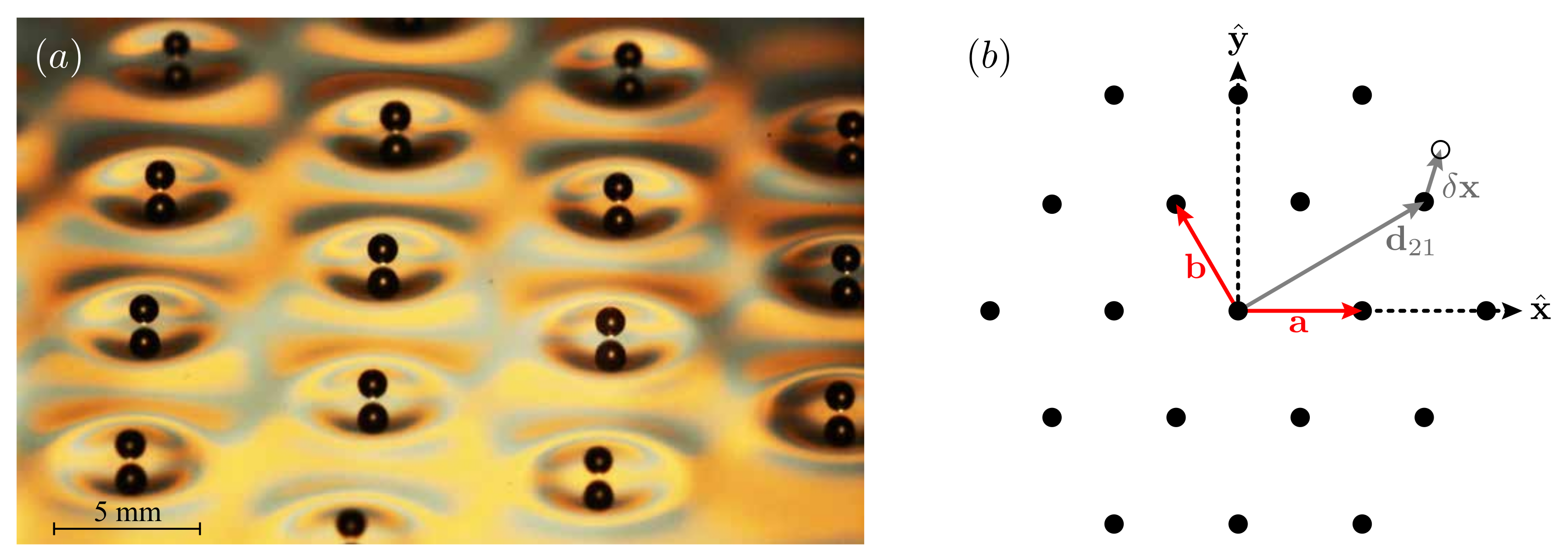
2.2. Base State of the Bravais Lattice

The unperturbed Bravais lattice has droplets located at horizontal positions

$${\mathit{d}}_{mn}=m\mathit{a}+n\mathit{b},$$

(6)

where m and n are integers and $\mathit{a}$ and $\mathit{b}$ are the basis vectors that define the lattice geometry, commonly referred to as ‘primitive vectors’ (see Figure 1b). We first demonstrate that a generic Bravais lattice is a stationary solution to Equation (4). Substituting ${\mathit{x}}_{mn}\left(t\right)={\mathit{d}}_{mn}$ into Equation (5) yields the wavefield for the Bravais lattice,

$$h(\mathit{x},t)=M_e\sum _{pq}\mathcal{S}(\gamma ,h\left({\mathit{d}}_{pq}\right))f\left(\right|\mathit{x}-{\mathit{d}}_{pq}\left|\right).$$

(7)

We note that the lattice symmetry ensures that all drops encounter the same wave height $h\left({\mathit{d}}_{pq}\right)=h_0$, so their phase factors are likewise identical, $\mathcal{S}\left(h_0\right)={\mathcal{S}}_0$. Evaluating Equation (7) at the lattice points yields an implicit expression for the local wave amplitude,

$$h_0=M_e\mathcal{S}(\gamma ,h_0)\sum _{pq}f\left(\left|{\mathit{d}}_{pq}\right|\right).$$

(8)

Making use of the functional form for $\mathcal{S}$ presented in Equation (A2), one may solve the implicit Equation (8) numerically to obtain $h_0$. Having obtained $h_0$, the phase parameters ${\mathcal{S}}_0=\mathcal{S}(\gamma ,h_0)$ and ${\mathcal{C}}_0=\mathcal{C}(\gamma ,h_0)$ may be computed using Equations (A2) and (A3), respectively. In Section 3, it will be shown that the values ${\mathcal{S}}_0$ and ${\mathcal{C}}_0$ depend on the initial geometry of the Bravais lattice, which in turn strongly influence the lattice stability.

Having solved for the base state wavefield, it is immediately evident that ${\mathit{x}}_{mn}\left(t\right)={\mathit{d}}_{mn}$ satisfies Equation (4) when $\nabla h({\mathit{d}}_{mn},t)=0$, which may be written explicitly as

$$\sum _{pq}{f}^{\prime }\left(\right|{\mathit{d}}_{pq}\left|\right)\frac{{\mathit{d}}_{pq}}{|{\mathit{d}}_{pq}|}=\mathbf{0}.$$

(9)

Physically, Equation (9) signifies that the net waveforce on each droplet must vanish, or equivalently that the slope of the wavefield beneath each droplet is zero. Noting that ${\mathit{d}}_{(-p,-q)}=-{\mathit{d}}_{(p,q)}$, the pairwise terms $(p,q)$ and $(-p,-q)$ cancel in Equation (9), leaving only the $(p,q)=(0,0)$ term which vanishes because the wave kernel is even and so $f^{\prime }\left(0\right)=0$ (see Equation (3)). It is thus apparent that, by virtue of its translational symmetry, any Bravais lattice is a stationary solution of the trajectory equation.

2.3. Dispersion Relation of the Perturbed Lattice

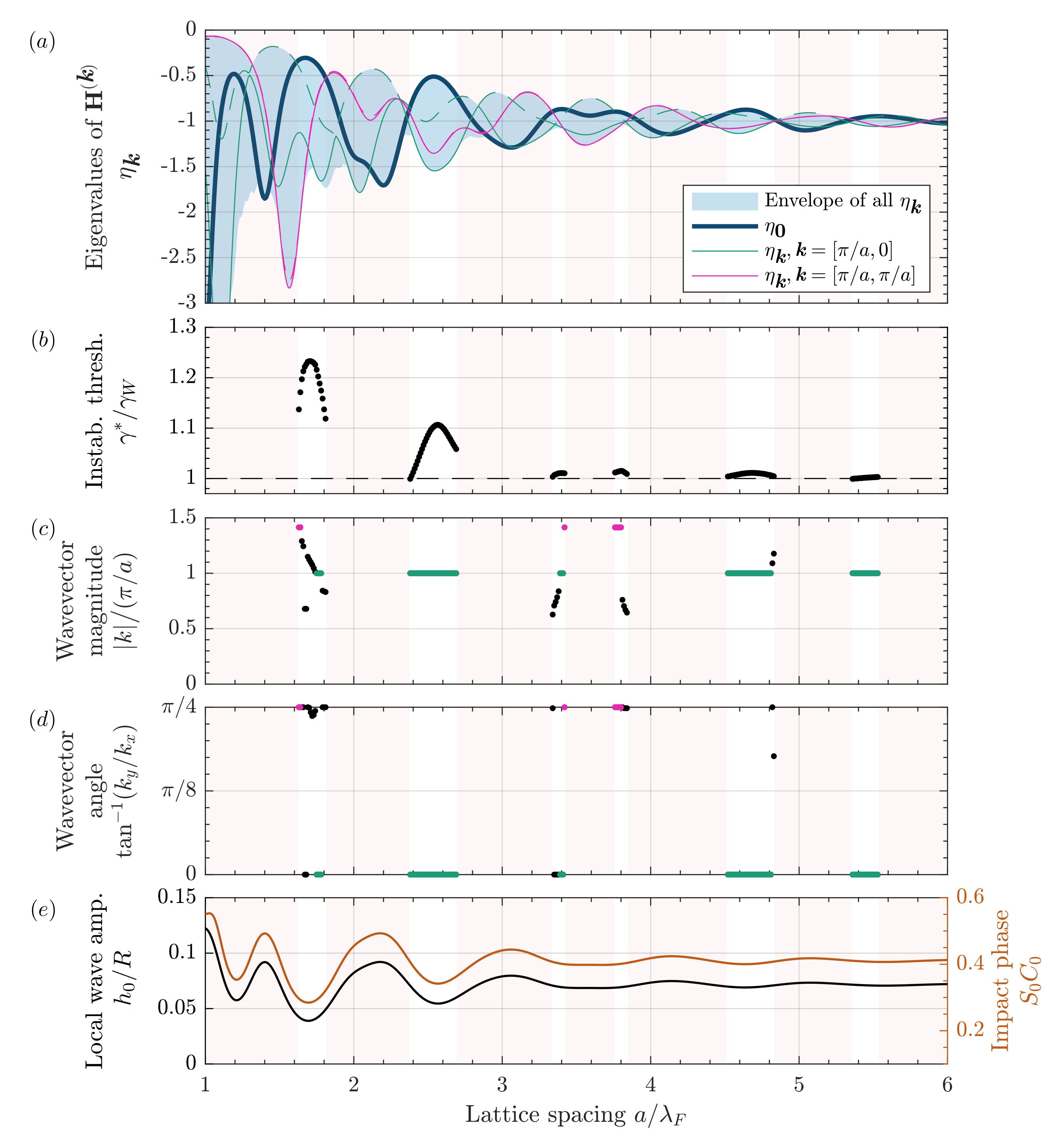
We may now assess the stability of the Bravais lattice by studying the growth of small perturbations to the base state, ${\mathit{x}}_{mn}\left(t\right)={\mathit{d}}_{mn}+\epsilon \delta {\mathit{x}}_{mn}\left(t\right)$, where $\epsilon \ll 1$. Substituting this perturbation into Equation (4), using the equilibrium condition (9), and expanding to first order in $\epsilon$, yields the following linearized equations of motion governing the perturbations $\delta {\mathit{x}}_{mn}\left(t\right)$,

$$\kappa {\ddot{\delta \mathit{x}}}_{mn}+{\dot{\delta \mathit{x}}}_{mn}=-\phi \sum _{pq}{\int }_{-\infty }^t{\mathbf{H}}_f\left({\mathit{d}}_{pq}\right)·\left(\delta {\mathit{x}}_{mn}\left(t\right)-\delta {\mathit{x}}_{pq}\left(s\right)\right)e^{-(t-s)/M_e}ds,$$

(10)

where

$$\phi =\beta {\mathcal{S}}_0{\mathcal{C}}_0,$$

(11)

and ${\mathbf{H}}_f$ denotes the Hessian matrix of the radially symmetric wave kernel f (Equation (3)),

$${\mathbf{H}}_f\left(\mathit{x}\right)={\left[\begin{array}{cc}\frac{{\partial }^{2}f}{\partial x^2}& \frac{{\partial }^{2}f}{\partial x\partial y}\\ \frac{{\partial }^{2}f}{\partial x\partial y}& \frac{{\partial }^{2}f}{\partial y^2}\end{array}\right]}_{\mathit{x}}.$$

(12)

The elements of ${\mathbf{H}}_f$ may be expressed explicitly as

$$\begin{array}{ccc}\hfill \frac{{\partial }^{2}f}{\partial x^2}\left(\mathit{x}\right)& =& \frac{f^{″}\left(r\right)}{r^2}{x}^2+\frac{f^{\prime }\left(r\right)}{r^3}{y}^2,\hfill \end{array}$$

(13)

$$\begin{array}{ccc}\hfill \frac{{\partial }^{2}f}{\partial y^2}\left(\mathit{x}\right)& =& \frac{f^{″}\left(r\right)}{r^2}{y}^2+\frac{f^{\prime }\left(r\right)}{r^3}{x}^2,\hfill \end{array}$$

(14)

$$\begin{array}{ccc}\hfill \frac{{\partial }^{2}f}{\partial x\partial y}\left(\mathit{x}\right)& =& \left(\frac{f^{″}\left(r\right)}{r^2}-\frac{f^{\prime }\left(r\right)}{r^3}\right)xy,\hfill \end{array}$$

(15)

where $\mathit{x}=(x,y)$ and $r=\left|\mathit{x}\right|$.

In deriving Equation (10), we note that variations in the phase parameters around the base values ${\mathcal{S}}_0$, ${\mathcal{C}}_0$ are of $\mathcal{O}\left({\epsilon }^2\right)$ and so can be neglected. To see this, note that

$$\mathcal{S}\left(\gamma ,h\left({\mathit{d}}_{mn}+ϵ\delta {\mathit{x}}_{mn}\right)\right)=\mathcal{S}\left(\gamma ,h\left({\mathit{d}}_{mn}\right)+\epsilon \nabla h\left({\mathit{d}}_{mn}\right)·\delta {\mathit{x}}_{mn}+\mathcal{O}\left({\epsilon }^2\right)\right),$$

(16)

but $\nabla h\left({\mathit{d}}_{mn}\right)=0$ in the base state (Equation (9)). Therefore, the impact phase parameters only enter our linear analysis through their base values ${\mathcal{S}}_0$, ${\mathcal{C}}_0$, which influence the resulting stability of the lattice through the parameter $\phi$ (Equation (11)) that scales the waveforce in Equation (10).

To derive the dispersion relation governing the linear stability of the lattice, we substitute the following normal mode perturbation into Equation (10)

$$\delta {\mathit{x}}_{mn}=\xi e^{i\mathit{k}·{\mathit{d}}_{mn}+{\omega }_{\mathit{k}}t}+\mathrm{c}.\mathrm{c}.,$$

(17)

where $\mathrm{c}.\mathrm{c}.$ denotes the complex conjugate of the preceding exponential term. Equation (17) represents a plane wave characterized by wavevector $\mathit{k}$, polarization vector $\xi$, and complex frequency ${\omega }_{\mathit{k}}$. The real and imaginary components of ${\omega }_{\mathit{k}}$ represent the mode’s growth rate and oscillation frequency, respectively. Making use of the following integral, ${\int }_{-\infty }^t{e}^{\omega s}{e}^{-(t-s)/M_e}ds=M_e{e}^{\omega t}/\left(1+M_e\omega \right)$, we thus obtain the dispersion relation

$$\underset{{\mathbf{D}}_{\mathit{k}}\left({\omega }_{\mathit{k}}\right)}{\underbrace{\left[\left(\kappa {\omega }_k^2+{\omega }_{\mathit{k}}\right)\mathbf{I}+\phi M_e\left({\mathbf{H}}^{\left(\mathbf{0}\right)}-\frac{{\mathbf{H}}^{\left(\mathit{k}\right)}}{1+M_e{\omega }_{\mathit{k}}}\right)\right]}}\xi =\mathbf{0},$$

(18)

where $\mathbf{I}$ denotes the identity matrix and

$${\mathbf{H}}^{\left(\mathit{k}\right)}=2\sum _{pq}{\mathbf{H}}_f\left({\mathit{d}}_{pq}\right)cos(\mathit{k}·{\mathit{d}}_{pq})$$

(19)

may be recognized as the elementwise discrete cosine transform of the Hessian matrix over the lattice. For $\mathit{k}=\mathbf{0}$, ${\mathbf{H}}^{\left(\mathbf{0}\right)}$ is the Hessian matrix of the net wavefield at the origin, as characterizes the wavefield’s local curvature.

Non-trivial solutions ($\xi \ne \mathbf{0}$) to the dispersion relation (18) exist when

$$det{\mathbf{D}}_{\mathit{k}}\left({\omega }_{\mathit{k}}\right)=0,$$

(20)

which takes the form of a sextic polynomial in the complex-valued frequency ${\omega }_{\mathit{k}}$ and may be solved numerically. If a wavevector $\mathit{k}$ exists such that any root ${\omega }_{\mathit{k}}^{*}$ of Equation (20) has a positive real part, then the associated mode will grow and the lattice will destabilize. If no such $\mathit{k}$ exist, the lattice remains stable. For an initially stable lattice, as the vibrational forcing $\gamma$ is increased, the instability threshold ${\gamma }^{*}$ is reached when there exists at least one ${\mathit{k}}^{*}$ such that $\mathrm{Re}\left({\omega }_{\mathit{k}}^{*}\right)\ge 0$. The polarization vector ${\xi }^{*}$ associated with the unstable mode ${\mathit{k}}^{*}$ may then be found by solving ${\mathbf{D}}_{\mathit{k}}\left({\omega }_{\mathit{k}}^{*}\right){\xi }^{*}=\mathbf{0}$ (Equation (18)). We note that the polarization vector $\xi$ must be real-valued as ${\mathbf{D}}_{\mathit{k}}$ is a symmetric matrix.

It is noteworthy that, owing to the discrete translational symmetry of the Bravais lattice, not all wavevectors $\mathit{k}$ produce physically distinguishable oscillations when substituted into the normal mode ansatz (17). For example, consider a square lattice characterized by ${\mathit{d}}_{mn}=a\left(m\widehat{\mathit{x}}+n\widehat{\mathit{y}}\right)$ and two wavevectors $\mathit{k}=\left(k_x,k_y\right)$ and ${\mathit{k}}^{\prime }=\left(k_x+2\pi /a,k_y+2\pi /a\right)$. Substituting ${\mathit{k}}^{\prime }$ into Equation (17) yields

$$\delta {\mathit{x}}_{mn}=\xi e^{2\pi i\left(m+n\right)}{e}^{i\mathit{k}·{\mathit{d}}_{mn}+{\omega }_{\mathit{k}}t}=\xi e^{i\mathit{k}·{\mathit{d}}_{mn}+{\omega }_{\mathit{k}}t},$$

(21)

an oscillation characterized by wavevector $\mathit{k}$. Therefore, ${\mathit{k}}^{\prime }$ and $\mathit{k}$ result in the same physical oscillation. It thus suffices to consider only wavevectors $\mathit{k}$ in the lattice’s so-called Brillouin zone, defined as the smallest set of $\mathit{k}$ required to describe all distinguishable vibrations of the discrete lattice [4]. The Brillouin zones for the square and triangular geometries considered in Section 3 are illustrated in Figure 2, and the procedure for generating the Brillouin zone for a generic Bravais lattice may be found in standard reference texts on solid-state physics [4].

3. Results

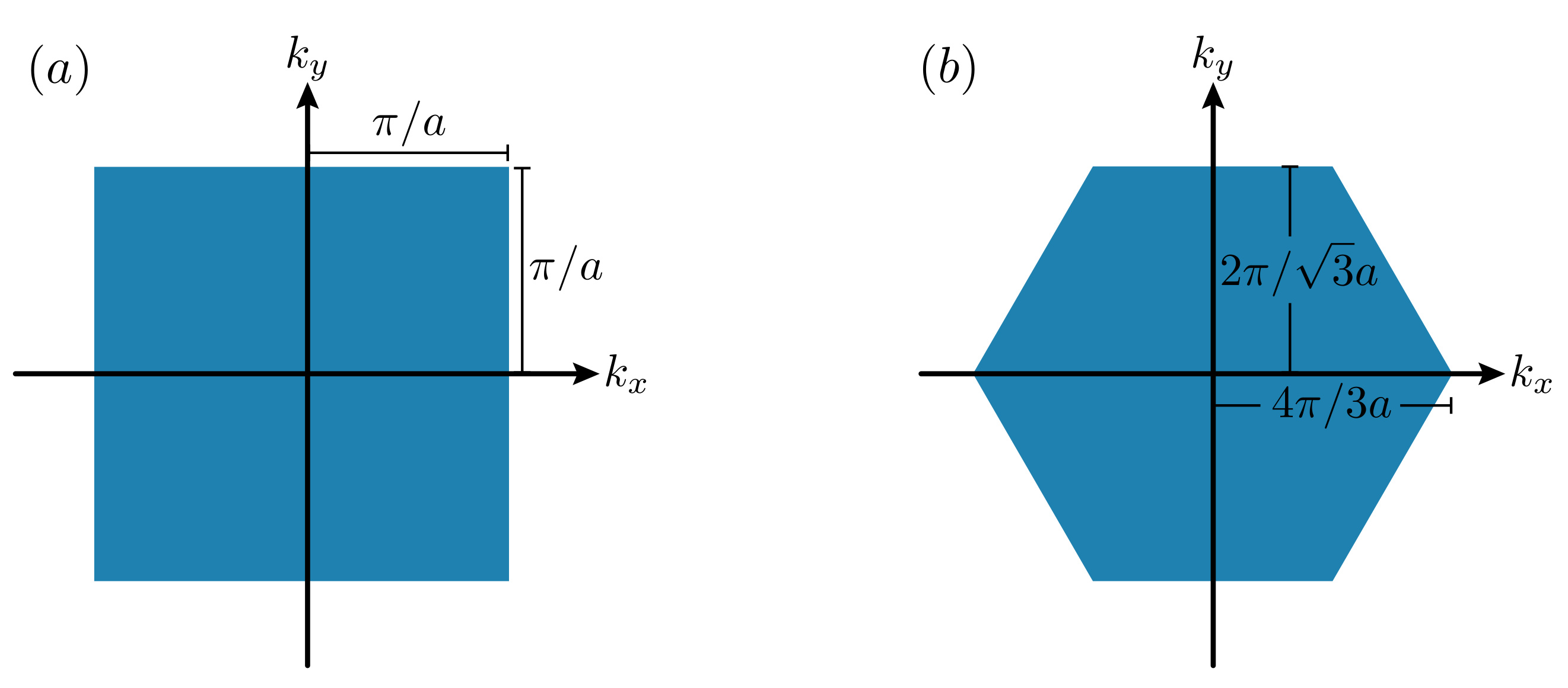
3.1. Square and Triangular Lattices

We first consider the stability of square and triangular lattices, as are characterized by a single inter-drop spacing a with droplets at the base state positions

$$\begin{array}{ccc}\hfill {\mathit{d}}_{mn}^{\left(\mathrm{square}\right)}& =& a\left(m\widehat{\mathit{x}}+n\widehat{\mathit{y}}\right),\hfill \end{array}$$

(22)

$$\begin{array}{ccc}\hfill {\mathit{d}}_{mn}^{\left(\mathrm{triangle}\right)}& =& a\left(m\widehat{\mathit{x}}+\left(n/2\right)\left(-\widehat{\mathit{x}}+\sqrt{3}\widehat{\mathit{y}}\right)\right),\hfill \end{array}$$

(23)

respectively. As is demonstrated in Appendix B, the four- and six-fold symmetry of the square and triangular geometries, respectively, result in the Hessian matrix for the net wavefield ${\mathbf{H}}^{\left(\mathbf{0}\right)}$ (Equation (19), with $\mathit{k}=\mathbf{0}$) reducing to a scalar multiple of the identity matrix $\mathbf{I}$,

$${\mathbf{H}}^{\left(\mathbf{0}\right)}={\eta }_{\mathbf{0}}\mathbf{I},$$

(24)

where ${\eta }_{\mathbf{0}}$ is the unique (repeated) eigenvalue of ${\mathbf{H}}^{\left(\mathbf{0}\right)}$. Geometrically, Equation (24) signifies that the curvature of the local wavefield beneath each droplet in the square and triangular base lattices is isotropic, having the same value in all horizontal directions. Using Equation (24), the general dispersion relation (18) reduces to the simpler eigenvalue problem,

$${\mathbf{H}}^{\left(\mathit{k}\right)}\xi =\left[\frac{1}{\phi M_e}\left(1+M_e{\omega }_{\mathit{k}}\right)\left(\kappa {\omega }_{\mathit{k}}^2+{\omega }_{\mathit{k}}+\phi {\eta }_{\mathbf{0}}{M}_e\right)\right]\xi ,$$

(25)

which admits non-trivial solutions when $\xi$ is an eigenvector of ${\mathbf{H}}^{\left(\mathit{k}\right)}$ with corresponding eigenvalue ${\eta }_{\mathit{k}}$. When such is the case, one may equate ${\eta }_{\mathit{k}}$ with the bracketed term on the right-hand side of Equation (25), yielding

$${\mathcal{P}}_1\left({\omega }_{\mathit{k}}\right)\equiv \kappa {\omega }_{\mathit{k}}^3+\left(1+\frac{\kappa }{M_e}\right){\omega }_{\mathit{k}}^2+\left(\frac{1}{M_e}+M_e\phi {\eta }_{\mathbf{0}}\right){\omega }_{\mathit{k}}+\phi \left({\eta }_{\mathbf{0}}-{\eta }_{\mathit{k}}\right)=0,$$

(26)

which may be solved for the three ${\omega }_{\mathit{k}}$ associated with each of the two eigenvalues ${\eta }_{\mathit{k}}$. Since $\kappa >0$ and ${\mathcal{P}}_1\left({\omega }_{\mathit{k}}\right)\to \infty$ as ${\omega }_{\mathit{k}}\to \infty$, the intermediate value theorem guarantees a positive real root whenever ${\mathcal{P}}_1\left(0\right)<0$, i.e., $\phi ({\eta }_{\mathbf{0}}-{\eta }_{\mathit{k}})<0$. We thus deduce that a lattice is always unstable if there are any wavevectors $\mathit{k}$ such that either eigenvalue ${\eta }_{\mathit{k}}$ of ${\mathbf{H}}^{\left(\mathit{k}\right)}$ is greater than ${\eta }_{\mathbf{0}}$.

Based on Equation (26), we now have a simple procedure for assessing whether a square or triangular lattice is unstable at the initial vibrational acceleration $\gamma =0.7{\gamma }_F$, which is below the walking threshold of a single drop ${\gamma }_W$ and corresponds approximately to the lowest $\gamma$ at which the droplets bounce in a period-doubled mode [52]. Specifically, we compute the eigenvalues ${\eta }_{\mathbf{0}}$ and ${\eta }_{\mathit{k}}$ of ${\mathbf{H}}^{\left(\mathit{k}\right)}$ (Equation (19)) numerically, noting that there are two ${\eta }_{\mathit{k}}$ for each wave vector $\mathit{k}$ in the Brillouin zone, and plot their dependence on the lattice spacing a for both the square (Figure 3a) and triangular (Figure 4a) lattice geometries. Intervals of a where ${\eta }_{\mathit{k}}>{\eta }_{\mathbf{0}}$ for all $\mathit{k}$ are shaded in red, indicating that the lattice is already unstable at $\gamma =0.7{\gamma }_F$. We observe that for both the square and triangular geometries, there are only discrete intervals of a for which the lattice is initially stable, which roughly correspond to geometries in which drops bounce in minima of the local wave amplitude (see Figure 3e and Figure 4e). We note that this behaviour is in accord with previous studies reporting that bound states are most stable when each drop bounces in a minimum of the net wavefield produced by its neighbours [32,33]. Thomson et al. [44] found similar swaths of initial instability as a function of the lattice spacing for infinite one-dimensional droplet chains at low vibrational accelerations, which they referred to as ‘geometric instabilities’.

For the set of lattices that are initially stable at $\gamma =0.7{\gamma }_F$, we may then determine the instability threshold ${\gamma }^{*}>0.7{\gamma }_F$ at which destabilization occurs. At ${\gamma }^{*}$, the real part of ${\omega }_{\mathit{k}}$ will vanish and the imaginary part will correspond to the frequency of the destabilizing oscillation. Substituting ${\omega }_{\mathit{k}}=i\mathsf{\Omega }$ ($\mathsf{\Omega }\in \mathbb{R}$) into Equation (26), separating the complex polynomial into real and imaginary parts, and eliminating $\mathsf{\Omega }$ yields

$${\mathcal{P}}_{\mathit{k}}\left(M_e\right)\equiv \phi {\eta }_{\mathbf{0}}{M}_e^3+\phi \kappa {\eta }_{\mathit{k}}{M}_e^2+M_e+\kappa =0.$$

(27)

Noting that $\kappa >0$, $\phi >0$ and ${\eta }_{\mathbf{0}}<0$, we observe that ${\mathcal{P}}_{\mathit{k}}\left(M_e\right)=0$ has at least one positive real root, the minimum of which corresponds to the memory $M_e^{*}$ at which the lattice destabilizes. Because ${\mathcal{Q}}_{\mathit{k}}\left(M_e\right)\equiv {\mathcal{P}}_{\mathit{k}}\left(M_e\right)-C{M}_e^2<{\mathcal{P}}_{\mathit{k}}\left(M_e\right)$ for every non-zero $M_e$ provided $C>0$, we infer that ${\mathcal{Q}}_{\mathit{k}}$ must have a root at a lower $M_e$ than does ${\mathcal{P}}_{\mathit{k}}$. Furthermore, if there is a wavevector ${\mathit{k}}^{\prime }$ such that ${\eta }_{{\mathit{k}}^{\prime }}<{\eta }_{\mathit{k}}$, then since ${\mathcal{P}}_{\mathit{k}}\left(M_e\right)-{\mathcal{P}}_{{\mathit{k}}^{\prime }}\left(M_e\right)=\phi \kappa M_e^2({\eta }_{\mathit{k}}-{\eta }_{{\mathit{k}}^{\prime }})>0$, the smallest real positive root of ${\mathcal{P}}_{{\mathit{k}}^{\prime }}\left(M_e\right)$ must be smaller than that of ${\mathcal{P}}_{\mathit{k}}\left(M_e\right)$. We thus conclude that the wave vector $\mathit{k}$ that goes unstable at the lowest memory value $M_e$, corresponds to that $\mathit{k}$ with the minimum eigenvalue ${\eta }_{\mathit{k}}$.

We may thus gain additional insight from the curves ${\eta }_{\mathit{k}}$ plotted in Figure 3a and Figure 4a for the square and triangular geometries, respectively. Namely, in the initially stable intervals of a, the lowermost curve ${\eta }_{\mathit{k}}$ corresponds to the destabilizing vibrational wavemode $\mathit{k}$ that will emerge at the instability threshold ${\gamma }^{*}$. In Figure 3 and Figure 4, we plot the instability thresholds ${\gamma }^{*}$ (panel b), and the magnitude and direction of the wavevector characterizing this destabilizing mode (panels c and d, respectively) as a function of the lattice spacing a. In all cases, we find that the polarization vector $\xi$ is parallel to the wave vector $\mathit{k}$, signifying that the lattices always destabilize into longitudinal, as opposed to transverse, oscillations.

For both the square and triangular geometries, the instability threshold of the lattice, ${\gamma }^{*}$, is almost always greater than the walking threshold ${\gamma }_W$ of a single drop. The lattices are most stable when the constituent drops bounce in the deepest minima of the wavefield produced by their neighbours, as was the case for droplet pairs and rings [32,33]. This effect is a direct result of variations in the impact phase, with the product ${\mathcal{S}}_0{\mathcal{C}}_0$ (see Equations (10) and (11)) decreasing with decreasing local wave amplitude (see Figure 3e and Figure 4e) and thus reducing the horizontal waveforce exerted on each droplet at impact. Conversely, we note that in their theoretical analysis of a one-dimensional lattice, Thomson et al. [44] predicted destabilization below ${\gamma }_W$, despite the fact that experimentally such lattices were found to remain stable above ${\gamma }_W$ [34]. This mismatch followed from their assumption of a constant impact phase, and highlights the importance of accounting for variations in the vertical dynamics by using a variable-impact-phase model when considering droplet–droplet interactions. In Figure 3b and Figure 4b we observe that ${\gamma }^{*}$ approaches ${\gamma }_W$ in the limit of large a, consistent with the droplets in the lattice becoming effectively uncoupled from their neighbours at sufficiently large distances.

In Figure 3c,d, we highlight two dominant modes of vibration for the square lattice, as are further illustrated in Figure 5. The first mode (green) corresponds to out-of-phase oscillations of neighbouring lattice planes along either the $\widehat{\mathit{x}}$ or $\widehat{\mathit{y}}$ directions, which are equivalent given the four-fold rotational symmetry of the square lattice. We note that Eddi et al. [43] observed a superposition of such oscillations in the $\widehat{\mathit{x}}$ and $\widehat{\mathit{y}}$ directions, resulting in the appearance of each droplet exhibiting roughly circular orbits around its base point (see Figure 4a of [43]). In magenta, we highlight a separate mode characterized by out-of-phase oscillations along 45 degree planes in the lattice with a wavelength of $\sqrt{2}a$, corresponding to the diagonal of a square cell. Apart from these two readily identifiable modes, the scaled wavevector $a\left|\mathit{k}\right|/\pi$ (Figure 3c) varies approximately linearly with the scaled lattice spacing $a/{\lambda }_F$, thus representing an oscillation wavelength that is no longer solely governed by a, but is now also influenced by the Faraday wavelength ${\lambda }_F$ that characterizes the underlying wavefield.

In Figure 4c,d, we highlight the dominant mode of vibration for the triangular lattice (magenta) which, as illustrated in Figure 6, corresponds to out-of-phase oscillations of neighbouring lattice planes along the $\pi /6$ direction (or equivalently, the $\pi /6+n\left(\pi /3\right)$, $n=\left(1,2,\cdots ,5\right)$ directions given the six-fold rotational symmetry of the lattice). This mode is consistent with that reported by Eddi et al. [43] (see Figure 4b of [43]). We note that in their experiments, Eddi et al. [43] used different drop sizes and fluid parameters than considered here, so we cannot present a quantitative comparison between their results and our theoretical predictions.

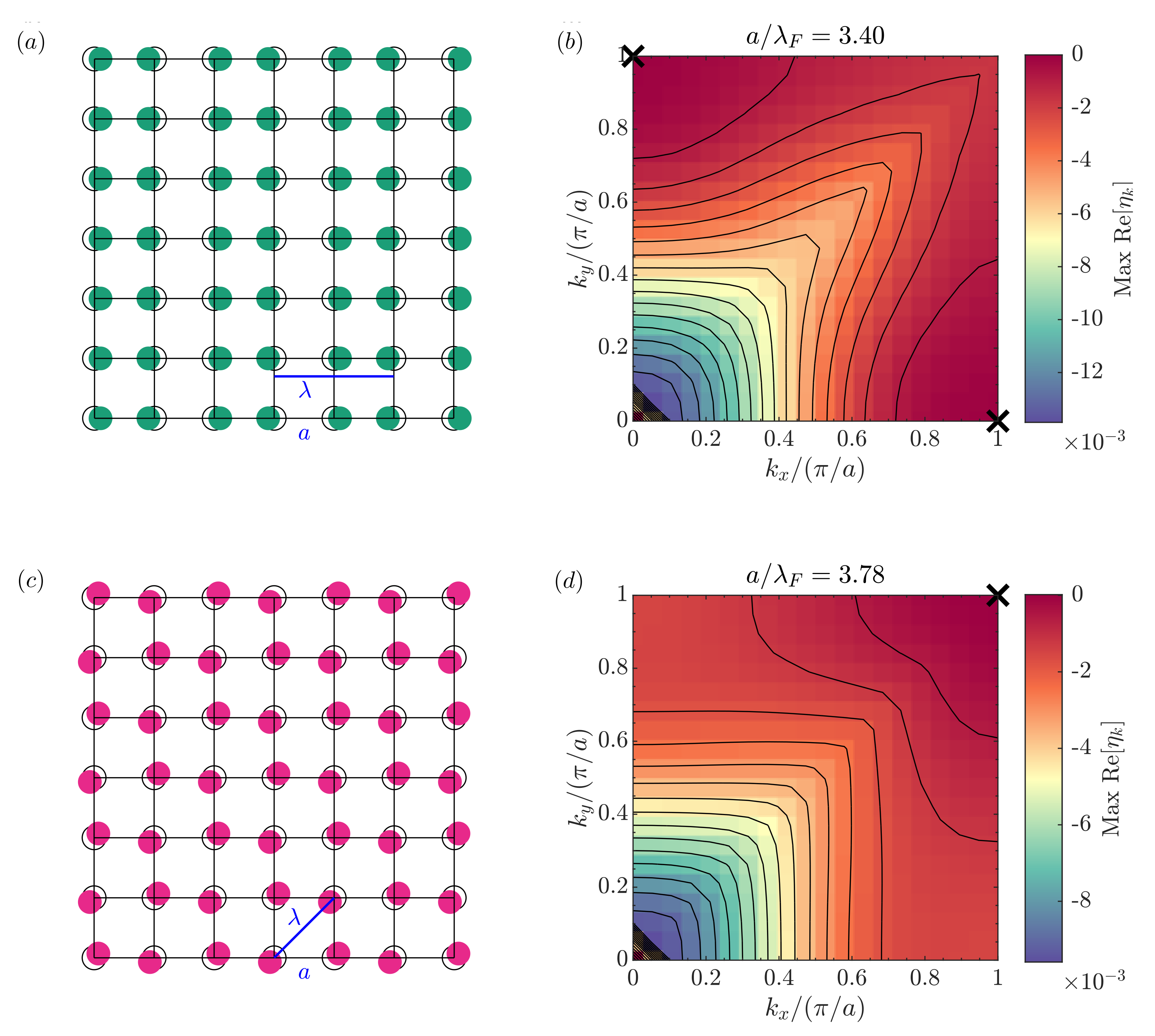
3.2. Geometric Instabilities in the Low-Memory Limit

We have demonstrated that, for the relatively low driving acceleration $\gamma =0.7{\gamma }_F$, square and triangular lattices are already unstable for certain values of the lattice spacing a. Following Thomson et al. [44], we refer to such lattices as being ‘geometrically unstable’. We proceed by demonstrating a method for predicting whether a generic Bravais lattice is geometrically unstable on the basis of the shape of the lattice-induced wavefield. In the low-memory limit $M_e\ll 1$, the dispersion relation (18) reduces to the eigenvalue problem

$$\left({\mathbf{H}}^{\left(\mathbf{0}\right)}-{\mathbf{H}}^{\left(\mathit{k}\right)}\right)\xi =\left[-\frac{1}{\phi M_e}\left(\kappa {\omega }_{\mathit{k}}^2+{\omega }_{\mathit{k}}\right)\right]\xi ,$$

(28)

which admits non-trivial solutions when $\xi$ is an eigenvector of the matrix $\left({\mathbf{H}}^{\left(\mathbf{0}\right)}-{\mathbf{H}}^{\left(\mathit{k}\right)}\right)$ with corresponding eigenvalue ${\alpha }_{\mathit{k}}$. When such is the case, one may equate ${\alpha }_{\mathit{k}}$ with the bracketed term on the right-hand side of Equation (28), yielding

$${\mathcal{P}}_2\left({\omega }_{\mathit{k}}\right)\equiv \kappa {\omega }_{\mathit{k}}^2+{\omega }_{\mathit{k}}+\phi M_e{\alpha }_{\mathit{k}}=0,$$

(29)

which may be solved to obtain the two ${\omega }_{\mathit{k}}$ associated with each of the two eigenvalues ${\alpha }_{\mathit{k}}$. We note that ${\mathcal{P}}_2\left({\omega }_{\mathit{k}}\right)\to \infty$ as ${\omega }_{\mathit{k}}\to \infty$. In the case ${\alpha }_{\mathit{k}}<0$, we also have ${\mathcal{P}}_2\left(0\right)<0$, and so the intermediate value theorem guarantees the existence of a positive real root. Therefore, ${\alpha }_{\mathit{k}}<0$ is a sufficient condition for the geometric instability of a generic Bravais lattice; while we have derived this result in the low-memory limit, one expects that increasing the memory will tend to promote lattice destabilization. Thus, a lattice that is geometrically unstable in the low-memory limit should remain so at higher memories.

In Figure 7, we use the above criterion to determine the regions of initial stability of a rectangular lattice, as is described by two lattice spacings a and b. We note that the diagonal line $a=b$ in Figure 7 yields the intervals of stability shown in Figure 3b. As was the case for the square and triangular geometries, the pockets of stability are correlated with minima in the local wave amplitude. Having identified the regions of initial stability, the dispersion relation (18) could then be used to characterize the instability threshold and most unstable vibrational mode for each lattice.

4. Discussion

We have used the variable-phase stroboscopic model of Couchman et al. [32] to consider the linear stability of a group of droplets arranged in a Bravais lattice. All Bravais lattices are stationary solutions to the stroboscopic model, since the lattice’s discrete translational symmetry ensures that the net waveforce on each droplet vanishes. By considering the response of the lattice to normal mode perturbations, our analysis yielded an implicit dispersion relation relating the vibrational mode’s wavevector $\mathit{k}$ to its complex frequency ${\omega }_{\mathit{k}}$, as captures both the mode’s growth rate and oscillation frequency. Particular attention was given to the square and triangular Bravais geometries, for which the rotational symmetry of the lattice allowed our general dispersion relation to be reduced to a form similar to that considered by Thomson et al. [44] in their investigation of a one-dimensional droplet chain. A distinctive feature of our analysis is the inclusion of variations in the drop’s vertical motion, as are required to capture the stabilizing influence of droplet–droplet interactions that allow lattices to remain stable above the walking threshold of the individual constituent drops. This stabilizing phenomenon has also been reported for a variety of other bound states [32,33,34,37,39].

While all lattices are stationary solutions to the trajectory equation, not all are stable at low vibrational accelerations; indeed, the majority are geometrically unstable [44]. For the square and triangular lattices, we deduced a criterion for geometric instability solely in terms of the local wave curvature beneath each droplet. This criterion predicts discrete intervals of stability in the lattice spacing. These stable regions correspond roughly to geometries that minimize the local wave amplitude beneath each droplet, a feature also reported in bound droplet pairs [32], rings [33], and one-dimensional lattices [44]. By considering the low-memory limit of our dispersion relation, we deduced a similar criterion for assessing the geometric instability of a generic Bravais lattice, which we used to identify the initial regions of stability for the rectangular lattice.

Consistent with the experimental observations reported by Eddi et al. [43], increasing the memory causes an initially stable lattice to destabilize into phonon-like motions characterized by coherent small-amplitude oscillations. The most unstable modes were longitudinal waves in all cases and were usually aligned along high-symmetry directions of the lattice; shear modes only destabilize at higher vibrational forcings. We numerically computed the instability threshold of the most unstable modes, and found that they typically arise above the walking threshold ${\gamma }_W$ for a single droplet, as highlights the stability imparted by neighbouring droplets. Furthermore, we found local maxima for the instability threshold at the centre of the initially stable regions, corresponding to minima in the local wave amplitude, a result not captured in the theoretical modelling of the one-dimensional lattice [44] where variable phase factors were neglected.

The hydrodynamic lattice exhibits certain features that are distinct from canonical models of phonons in crystalline lattices, such as those analysed by Blackman [53] and Montroll [54]. In these models, a discrete lattice of masses is connected to their nearest and next-nearest neighbours via a linear spring force. If we were to remove the damping term from our dispersion relation (18), and take the low-memory limit considered in Section 3.2, we would recover a dispersion relation of the same form as that of Blackman and Montroll, for which all modes are neutrally stable. For droplet lattices accessible in the laboratory, the damping term in the trajectory Equation (1) dominates the inertia term in the low-memory limit, resulting in overdamped oscillations. In our system, neutrally stable oscillations only arise when the stabilizing effects of damping precisely balance the destabilizing effects of memory.

In the low-memory limit, the potential landscape is a sum of wave kernels centred at each droplet of the lattice. This potential induces a linear spring force with the local curvature playing the role of the spring constant. Since the wave kernel is oscillatory, an individual droplet may contribute a negative curvature (analogously, a negative spring constant) to this sum, depending on the inter-droplet distance. This effect is not seen in a canonical mass-spring lattice, as the springs are only perturbed about their equilibrium lengths. The oscillatory wave kernel of the hydrodynamic lattice thus gives rise to much richer dynamics than arise in generic crystal lattices, including the discrete windows of initial stability.

Our linear theory for the hydrodynamic lattice cannot predict the amplitude of the emergent oscillations. A weakly nonlinear extension of our theory, which parallels that developed for a one-dimensional hydrodynamic lattice [46], could yield insight into the more complex oscillations reported by Eddi et al. [43]. The potential for further theoretical explorations abound. For example, one might consider how the introduction of defects, such as holes or an additional droplet, might modify the resulting lattice dynamics [55].

In solid-state physics, more complex lattice geometries arise, for example, in ionic lattices comprised of more than one type of atom. In such cases, the ‘unit cell’ constitutes the smallest non-repeating subcomponent of the lattice, and the structure may be defined in terms of a Bravais lattice of such unit cells. As is well established in the phonon literature, having more than one element per unit cell is a prerequisite for optical modes and band gaps [4,56], frequency ranges in which no vibrational states arise. In our study, we restricted our attention to the case where there is a single droplet per unit cell, and focused on relatively simple geometries. In the future, one might extend this framework to describe lattices tiled by unit cells containing multiple droplets, thereby describing arbitrary lattices in the plane. We note that for such arrangements, the equilibrium condition $\nabla h\left({\mathit{d}}_{mn}\right)=0$ (Equation (9)) would not necessarily be satisfied for all arbitrary unit cells. Nevertheless, an extended theoretical framework might enable an investigation of the Archimedian tilings that Eddi et al. [42] were unable to access in the laboratory, such as the truncated hexagonal and great rhombi-trihexagonal lattices.

References

1. Krumhansl, J. Lattice vibrations in solids. J. Appl. Phys. 1962, 33, 307–319. [Google Scholar] [CrossRef]
2. Cochran, W. Lattice vibrations. Rep. Prog. Phys. 1963, 26, 1. [Google Scholar] [CrossRef]
3. Dean, P. Atomic vibrations in solids. IMA J. Appl. Math. 1967, 3, 98–165. [Google Scholar] [CrossRef]
4. Kittel, C. Introduction to Solid State Physics; Wiley: Hoboken, NJ, USA, 1996. [Google Scholar]
5. Kane, C.; Lubensky, T. Topological boundary modes in isostatic lattices. Nat. Phys. 2014, 10, 39–45. [Google Scholar] [CrossRef]
6. Lubensky, T.; Kane, C.; Mao, X.; Souslov, A.; Sun, K. Phonons and elasticity in critically coordinated lattices. Rep. Prog. Phys. 2015, 78, 073901. [Google Scholar] [CrossRef]
7. Nash, L.M.; Kleckner, D.; Read, A.; Vitelli, V.; Turner, A.M.; Irvine, W.T. Topological mechanics of gyroscopic metamaterials. Proc. Natl. Acad. Sci. USA 2015, 112, 14495–14500. [Google Scholar] [CrossRef]
8. Süsstrunk, R.; Huber, S.D. Classification of topological phonons in linear mechanical metamaterials. Proc. Natl. Acad. Sci. USA 2016, 113, E4767–E4775. [Google Scholar] [CrossRef]
9. Bragg, W.L.; Nye, J.F. A dynamical model of a crystal structure. Proc. R. Soc. A 1947, 190, 474–481. [Google Scholar]
10. Penciu, R.; Kriegs, H.; Petekidis, G.; Fytas, G.; Economou, E. Phonons in colloidal systems. J. Chem. Phys. 2003, 118, 5224–5240. [Google Scholar] [CrossRef]
11. Keim, P.; Maret, G.; Herz, U.; von Grünberg, H.H. Harmonic lattice behavior of two-dimensional colloidal crystals. Phys. Rev. Lett. 2004, 92, 215504. [Google Scholar] [CrossRef]
12. Kaya, D.; Green, N.; Maloney, C.; Islam, M. Normal modes and density of states of disordered colloidal solids. Science 2010, 329, 656–658. [Google Scholar] [CrossRef]
13. Chen, K.; Still, T.; Schoenholz, S.; Aptowicz, K.B.; Schindler, M.; Maggs, A.; Liu, A.J.; Yodh, A. Phonons in two-dimensional soft colloidal crystals. Phys. Rev. E 2013, 88, 022315. [Google Scholar] [CrossRef]
14. Ghosh, A.; Mari, R.; Chikkadi, V.; Schall, P.; Maggs, A.; Bonn, D. Low-energy modes and Debye behavior in a colloidal crystal. Phys. A Stat. Mech. Its Appl. 2011, 390, 3061–3068. [Google Scholar] [CrossRef]
15. Beatus, T.; Tlusty, T.; Bar-Ziv, R. Phonons in a one-dimensional microfluidic crystal. Nat. Phys. 2006, 2, 743–748. [Google Scholar] [CrossRef]
16. Schiller, U.D.; Fleury, J.B.; Seemann, R.; Gompper, G. Collective waves in dense and confined microfluidic droplet arrays. Soft Matter 2015, 11, 5850–5861. [Google Scholar] [CrossRef]
17. Tsang, A.C.H.; Shelley, M.J.; Kanso, E. Activity-induced instability of phonons in 1D microfluidic crystals. Soft Matter 2018, 14, 945–950. [Google Scholar] [CrossRef]
18. Ono-dit-Biot, J.C.; Soulard, P.; Barkley, S.; Weeks, E.R.; Salez, T.; Raphaël, E.; Dalnoki-Veress, K. Mechanical properties of 2D aggregates of oil droplets as model mono-crystals. Soft Matter 2021, 17, 1194–1201. [Google Scholar] [CrossRef]
19. Benjamin, T.B.; Ursell, F. The stability of the plane free surface of a liquid in vertical periodic motion. Proc. R. Soc. A 1954, 225, 505–515. [Google Scholar]
20. Miles, J.; Henderson, D. Parametrically forced surface waves. Annu. Rev. Fluid Mech. 1990, 22, 143–165. [Google Scholar] [CrossRef]
21. Walker, J. The amateur scientist. Drops of liquid can be made to float on liquid. What enables them to do so? Sci. Am. 1978, 238, 151. [Google Scholar] [CrossRef]
22. Couder, Y.; Fort, E.; Gautier, C.H.; Boudaoud, A. From bouncing to floating: Noncoalescence of drops on a fluid bath. Phys. Rev. Lett. 2005, 94, 177801. [Google Scholar] [CrossRef] [PubMed]
23. Moláček, J.; Bush, J.W.M. Drops bouncing on a vibrating bath. J. Fluid Mech. 2013, 727, 582–611. [Google Scholar] [CrossRef]
24. Couder, Y.; Protiere, S.; Fort, E.; Boudaoud, A. Dynamical phenomena: Walking and orbiting droplets. Nature 2005, 437, 208. [Google Scholar] [CrossRef] [PubMed]
25. Protière, S.; Boudaoud, A.; Couder, Y. Particle–wave association on a fluid interface. J. Fluid Mech. 2006, 554, 85–108. [Google Scholar] [CrossRef]
26. Eddi, A.; Sultan, E.; Moukhtar, J.; Fort, E.; Rossi, M.; Couder, Y. Information stored in Faraday waves: The origin of a path memory. J. Fluid Mech. 2011, 674, 433–463. [Google Scholar] [CrossRef]
27. Fort, E.; Eddi, A.; Boudaoud, A.; Moukhtar, J.; Couder, Y. Path-memory induced quantization of classical orbits. Proc. Natl. Acad. Sci. USA 2010, 107, 17515–17520. [Google Scholar] [CrossRef]
28. Bush, J.W.M. Pilot-wave hydrodynamics. Annu. Rev. Fluid Mech. 2015, 47, 269–292. [Google Scholar] [CrossRef]
29. Bush, J.W.M.; Couder, Y.; Gilet, T.; Milewski, P.A.; Nachbin, A. Introduction to focus issue on hydrodynamic quantum analogs. Chaos Interdiscip. J. Nonlinear Sci. 2018, 28, 096001. [Google Scholar] [CrossRef]
30. Bush, J.W.M.; Oza, A.U. Hydrodynamic quantum analogs. Rep. Prog. Phys. 2020, 84, 017001. [Google Scholar] [CrossRef]
31. Rahman, A.; Blackmore, D. Walking droplets through the lens of dynamical systems. Mod. Phys. Lett. B 2020, 34, 2030009. [Google Scholar] [CrossRef]
32. Couchman, M.M.P.; Turton, S.E.; Bush, J.W.M. Bouncing phase variations in pilot-wave hydrodynamics and the stability of droplet pairs. J. Fluid Mech. 2019, 871, 212–243. [Google Scholar] [CrossRef]
33. Couchman, M.M.P.; Bush, J.W.M. Free rings of bouncing droplets: Stability and dynamics. J. Fluid Mech. 2020, 903. [Google Scholar] [CrossRef]
34. Thomson, S.J.; Couchman, M.M.P.; Bush, J.W.M. Collective vibrations of confined levitating droplets. Phys. Rev. Fluids 2020, 5, 083601. [Google Scholar] [CrossRef]
35. Barnes, L.; Pucci, G.; Oza, A.U. Resonant interactions in bouncing droplet chains. C. R. Mécanique 2020, 348, 573–589. [Google Scholar] [CrossRef]
36. Protière, S.; Bohn, S.; Couder, Y. Exotic orbits of two interacting wave sources. Phys. Rev. E 2008, 78, 036204. [Google Scholar] [CrossRef]
37. Oza, A.U.; Siéfert, E.; Harris, D.M.; Moláček, J.; Bush, J.W.M. Orbiting pairs of walking droplets: Dynamics and stability. Phys. Rev. Fluids 2017, 2, 053601. [Google Scholar] [CrossRef]
38. Borghesi, C.; Moukhtar, J.; Labousse, M.; Eddi, A.; Fort, E.; Couder, Y. Interaction of two walkers: Wave-mediated energy and force. Phys. Rev. E 2014, 90, 063017. [Google Scholar] [CrossRef]
39. Arbelaiz, J.; Oza, A.U.; Bush, J.W.M. Promenading pairs of walking droplets: Dynamics and stability. Phys. Rev. Fluids 2018, 3, 013604. [Google Scholar] [CrossRef]
40. Lieber, S.I.; Hendershott, M.C.; Pattanaporkratana, A.; Maclennan, J.E. Self-organization of bouncing oil drops: Two-dimensional lattices and spinning clusters. Phys. Rev. E 2007, 75, 056308. [Google Scholar] [CrossRef]
41. Eddi, A.; Terwagne, D.; Fort, E.; Couder, Y. Wave propelled ratchets and drifting rafts. Europhys. Lett. 2008, 82, 44001. [Google Scholar] [CrossRef]
42. Eddi, A.; Decelle, A.; Fort, E.; Couder, Y. Archimedean lattices in the bound states of wave interacting particles. Europhys. Lett. 2009, 87, 56002. [Google Scholar] [CrossRef]
43. Eddi, A.; Boudaoud, A.; Couder, Y. Oscillating instability in bouncing droplet crystals. Europhys. Lett. 2011, 94, 20004. [Google Scholar] [CrossRef]
44. Thomson, S.J.; Durey, M.; Rosales, R.R. Collective vibrations of a hydrodynamic active lattice. Proc. R. Soc. A 2020, 476, 20200155. [Google Scholar] [CrossRef]
45. Oza, A.U.; Rosales, R.R.; Bush, J.W.M. A trajectory equation for walking droplets: Hydrodynamic pilot-wave theory. J. Fluid Mech. 2013, 737, 552–570. [Google Scholar] [CrossRef]
46. Thomson, S.J.; Durey, M.; Rosales, R.R. Discrete and periodic complex Ginzburg-Landau equation for a hydrodynamic active lattice. Phys. Rev. E 2021, 103, 062215. [Google Scholar] [CrossRef]
47. Moláček, J.; Bush, J.W.M. Drops walking on a vibrating bath: Towards a hydrodynamic pilot-wave theory. J. Fluid Mech. 2013, 727, 612–647. [Google Scholar] [CrossRef]
48. Turton, S.E.; Couchman, M.M.P.; Bush, J.W.M. A review of the theoretical modeling of walking droplets: Towards a generalized pilot-wave framework. Chaos Interdiscip. J. Nonlinear Sci. 2018, 28, 096111. [Google Scholar] [CrossRef]
49. Harris, D.M.; Quintela, J.; Prost, V.; Brun, P.T.; Bush, J.W.M. Visualization of hydrodynamic pilot-wave phenomena. J. Vis. 2017, 20, 13–15. [Google Scholar] [CrossRef]
50. Damiano, A.P.; Brun, P.T.; Harris, D.M.; Galeano-Rios, C.A.; Bush, J.W.M. Surface topography measurements of the bouncing droplet experiment. Exp. Fluids 2016, 57, 163. [Google Scholar] [CrossRef]
51. Tadrist, L.; Shim, J.B.; Gilet, T.; Schlagheck, P. Faraday instability and subthreshold Faraday waves: Surface waves emitted by walkers. J. Fluid Mech. 2018, 848, 906–945. [Google Scholar] [CrossRef]
52. Wind-Willassen, Ø.; Moláček, J.; Harris, D.M.; Bush, J.W.M. Exotic states of bouncing and walking droplets. Phys. Fluids 2013, 25, 082002. [Google Scholar] [CrossRef]
53. Blackman, M. Contributions to the theory of the specific heat of crystals II—On the vibrational spectrum of cubical lattices and its application to the specific heat of crystals. Proc. R. Soc. A 1935, 148, 384–406. [Google Scholar]
54. Montroll, E.W. Dynamics of a square lattice I. Frequency spectrum. J. Chem. Phys. 1947, 15, 575–591. [Google Scholar] [CrossRef]
55. Bell, R. The dynamics of disordered lattices. Rep. Prog. Phys. 1972, 35, 1315–1409. [Google Scholar] [CrossRef]
56. Kosevich, A.M. The Crystal Lattice: Phonons, Solitons, Dislocations, Superlattices; John Wiley & Sons: Hoboken, NJ, USA, 2006. [Google Scholar]
Figure 1. (a) An oblique view of a triangular lattice of millimetric droplets bouncing on the surface of a vertically vibrating liquid bath. The droplets are coupled by a shared wavefield, as is visualized by illuminating the bath with a striped pattern of coloured light [49]. We note that beneath each drop, the drop’s reflection from the bath surface is visible. (b) A Bravais lattice is generated via enumeration of the points d m n = m a + n b , ( m , n ) Z , with point ( m , n ) = ( 2 , 1 ) highlighted for illustration. The basis vectors describing the triangular lattice shown here are a = a ( 1 , 0 ) and b = a ( 1 / 2 , 3 / 2 ) , where a has units of length and sets the lattice spacing. We study the response of the lattice to perturbations δ x away from its base state.
Symmetry 14 01524 g001
Figure 2. The extent of the Brillouin zone in wavevector space ( k x , k y ) for (a) square and (b) triangular Bravais lattices with lattice spacing a [4]. Wavevectors k outside the Brillouin zone are paired with an equivalent k within the Brillouin zone such that k and k yield the same physical vibration once substituted into the normal mode ansatz (17), a result of the discrete translational symmetry of the lattice. In characterizing lattice stability, it thus suffices to consider only modes with wavevectors k within the Brillouin zone.
Symmetry 14 01524 g002
Figure 3. The square lattice. (a) The eigenvalues η k of the matrix H ( k ) (19), governing the lattice stability, are plotted as a function of the inter-drop spacing a, normalized by the Faraday wavelength λ F . In intervals of a where η 0 is greater than all η k , the lattice is initially stable at γ / γ F = 0.7 . Otherwise, the lattice is already unstable as denoted by red shading. Curves η k for two common modes of instability are highlighted. There are two eigenvalues η k for a single mode k , denoted by dashed and solid lines of the same colour. We note that the two magenta curves are virtually indistinguishable. For a given a, the most negative η k corresponds to the destabilizing wave mode. (b) The instability threshold γ * , normalized by the walking threshold for a single drop γ W , for initially stable spacings a. The corresponding wavevector magnitude k , normalized by π / a (see Figure 2a), and wave angle with respect to the x-axis, are shown for the destabilizing mode in panels (c,d), respectively. Green and magenta points indicate spacings a where one of the two wave modes highlighted in panel (a) are found to be destabilizing. These modes are further illustrated in Figure 5. (e) The black curve indicates the dependence on lattice spacing of the local wave amplitude h 0 beneath each droplet in the base lattice, normalized by the drop radius R. The orange curve denotes the corresponding product of impact phases S 0 C 0 that influences the lattice stability through φ in Equation (10).
Symmetry 14 01524 g003
Figure 4. The triangular lattice. Quantities characterizing the stability of a triangular lattice are plotted as a function of the lattice spacing a, in the same manner as for the square lattice in Figure 3. The dominant mode of instability is highlighted in magenta in panels (c,d), and is illustrated in Figure 6.
Symmetry 14 01524 g004
Figure 5. Common vibrational modes of the square lattice corresponding to longitudinal waves along high-symmetry lattice directions. (a) An illustration of the k = ( π / a , 0 ) wave mode highlighted by green markers in Figure 3, corresponding to the out-of-phase oscillations of neighbouring planes along the x ^ direction with wavelength λ = 2 a . (b) The maximum real part of the eigenvalues η k are shown for a lattice spacing a / λ F = 3.40 , with the most unstable modes k = ( π / a , 0 ) and ( 0 , π / a ) marked by crosses. (c,d) Analogous plots for the wave mode k = ( π / a , π / a ) , highlighted by magenta markers in Figure 3, corresponding to the out-of-phase oscillations of neighbouring planes along the 45 degree diagonal, with wavelength λ = 2 a .
Symmetry 14 01524 g005
Figure 6. Common vibrational mode of the triangular lattice. (a) An illustration of the k = 2 π 3 a ( 3 2 , 1 2 ) wave mode highlighted by magenta markers in Figure 4, corresponding to the out-of-phase oscillations of neighbouring planes along a line 30 degrees to the horizontal, with wavelength λ = 3 a . (b) The maximum real part of the eigenvalues η k for the lattice spacing a / λ F = 2.5 . The Brillouin zone boundary is traced in black (see Figure 2b), and crosses indicate the most unstable modes: k = 2 π 3 a ( 3 2 , 1 2 ) and π / 3 rotations thereof.
Symmetry 14 01524 g006
Figure 7. The rectangular lattice is parameterised by two lattice spacings, a and b. Regions of initial stability at low memory are shaded in green. All other lattices are geometrically unstable. The colourmap corresponds to the local wave amplitude beneath each drop h 0 , normalized by the drop radius R. Stable regions are roughly correlated with minima in h 0 . The diagonal line a = b corresponds to the square lattice, where the regions of initial stability correspond to those presented in Figure 3.
Symmetry 14 01524 g007