Computer Simulation of the Seismic Wave Propagation in Poroelastic Medium

Abstract

This article presents an algorithm for the numerical solution of an initial-boundary value problem for a symmetric t-hyperbolic system of partial differential equations. This problem is based on continual filtration model, which describes the propagation of seismic waves in a poroelastic medium saturated with a fluid characterized by such physical parameters as the propagation velocities of longitudinal P- (fast and slow) and transverse S-waves, the density of the medium materials, and porosity. The system of linearized equations of saturated porous media is formulated in terms of physical variables of the velocity–stress tensor of the porous matrix and the velocity–pressure of the saturating fluid in the absence of energy dissipation. The solution is implemented numerically using an explicit finite difference upwind scheme built on a staggered grid to avoid the appearance of oscillations in the solution functions. The program code implementing parallel computing is developed in the high-performance Julia programming language. The possibility of using the approach is demonstrated by the example of solving the problem of propagation of seismic waves from a source located in the formation. Computational experiments based on real data from oil reservoirs have been implemented, and dynamic visualization of solutions consistent with the first waves arrival times has been obtained.

1. Introduction

Mathematical modeling plays an essential role in the development of new geophysical technologies, which makes it possible to provide synthetic wave fields for various arrangements of sources and receivers of acoustic vibrations in models of media with a given complexity of internal structure. Computer modeling is especially important in view of the complexity of conducting an experimental study of internal non-stationary physical processes in fluid-saturated elastically deformable porous structures [1,2]. The development of computer simulation methods for realistic models of filtration mechanics in geophysical applications stimulates progress in many other fields of research, such as medicine, biotechnology, materials science, chemistry, micro- and nanofluidics, and geosciences [3,4,5,6,7]. Hyperbolic systems of partial differential equations are found in modeling separation and reaction engineering problems.

The main approach to the study of wave processes in liquid-saturated porous media is based on the Frenkel–Biot theory [8,9]. The model, which describes the processes of deformation of an elastic porous medium and the flow of fluid in it, is macroscopic, i.e., assumes that the space is filled with an enclosing poroelastic two-phase medium, and the phases corresponding to the porous solid and the liquid contained in the pores are present at each point in space. The Frenkel–Biot type models consist of two groups of equations: (I) equations of the theory of elasticity taking into account the internal forces associated with the influence of fluid pressure in pores on the stress-strain state of the medium, and (II) equations of fluid filtration in pores taking into account changes in the volume of the pore space filled with fluid due to deformation of the medium.

A continuum filtration model that satisfies the laws of thermodynamics was proposed in [10,11]. In this theory, the properties of a saturated porous medium are described using such physical parameters as the propagation velocities of two longitudinal waves and one transverse acoustic wave, the partial densities of the porous matrix and the saturating liquid, and the permeability coefficient. The continuum filtration approach makes it possible to describe the poroelastic medium with a smaller number of model parameters than in the Frenkel–Biot theory of poroelasticity and with a better agreement with experimental data [12].

The main tool for studying the applied problems of the theory of poroelasticity is numerical modeling, which allows conduction of numerical experiments with fully controlled input data and thereby reliably verifying hypotheses and formulating criteria for the manifestation of fluid mobility in seismic data. In [13,14,15,16,17,18,19,20,21,22,23,24,25], the propagation of seismic waves in porous media in the presence of energy dissipation was studied. Finite difference methods for solving poroelasticity problems have been formulated in several ways. In [13,14], the central difference method was used in terms of displacements. A semi-analytical method for solving a system of poroelasticity equations in terms of displacements is proposed in [15,16]. In [17], the problem was investigated by means of a predictor-corrector scheme for a system of velocity-stress equations. In [20], a spectral method was used, where the time derivatives are approximated through Laguerre functions (polynomials). The numerical solution of linear two-dimensional dynamic problems for porous media by the finite difference method together with the discrete PML model was used in [19] for the absorbing boundaries. The PML is introduced by Berenger (1994) for electromagnetism. Many authors have applied the PML to various wavefields simulations: Zeng et al. (2001) analyzed the PML in numerical modeling of the poroelastic media in time domain [14]. In [2], the PML is applied to the poroelastic waves in frequency domain and is used for the absorbing boundaries. The simplified wave equation with the PML attenuation term in time domain is used in [3]. Computational algorithms based on the finite element method have been successfully used to simulate the dynamics of hydraulic fracturing crack development in a three-dimensional formulation [26]. The development of multiprocessor systems stimulated the development of computational methods for solving seismic problems [27,28]. The grid-characteristic numerical method, which takes into account the internal mathematical structure of the hyperbolic problem—the propagation of discontinuities along the characteristics—has been successfully applied to the numerical solution of the direct problem of wave propagation in a heterophase medium [29].

In this paper, a numerical solution of the dynamic poroelasticity problem is obtained within the framework of a continuous filtration model. The features of the discretization of linearized poroelasticity equations of physical variables are considered. A feature of the model of a homogeneous, isotropic liquid-saturated porous medium is the specification of its properties by experimentally measurable velocities of longitudinal fast and slow P and transverse S acoustic waves in a two-phase medium. The difference algorithm is based on the finite difference method using an upwind staggered difference scheme to avoid the appearance of oscillations in solution functions [30]. The implementation of the scheme is sufficiently universal for calculations on a rectangular grid with the setting of various boundary conditions for pressure and stresses. The program code for the implementation of the algorithm was developed using the high-performance Julia programming language, since the explicit computational scheme allows efficient parallelization of cyclic sections of the algorithm. The stability of the scheme is ensured by selecting the grid steps in time and in spatial variables to satisfy the Friedrichs–Courant–Lewy criterion. The possibilities of the approach used are demonstrated by two examples of numerical experiments using realistic sets of parameter values and types of functions describing a seismic source. A visualization of the solution describing the change in the velocity of propagation of seismic waves in a poroelastic formation is obtained.

2. Material and Methods

2.1. Statement of the Problem

Let us turn to the mathematical formulation of the continuum model for a two-dimensional dynamic problem. It is expressed as the initial-boundary problem for a symmetric t-hyperbolic system. The main equations are based on the laws of momentum conservation, Hooke’s laws, and are consistent with the thermodynamics conditions. A half-plane filled with a liquid-saturated porous medium is considered, with parameters characterizing each of the components of such a medium.

It is assumed that the liquid completely fills the pores. The distribution of phases in space is described by such a macroscopic parameter as porosity (the volume concentration of voids filled with fluid in the medium).

The propagation of seismic waves in these media in the absence of energy loss is described by the following initial-boundary value problem in terms of the velocity components of the saturating fluid, the velocity of the solid matrix, the fluid pressure, and the stress tensor [19,20,21,22,24,25]. The values related to the solid phase of the elastic medium are denoted by the subscript “s”, and to the mobile phase of the saturating liquid—by the subscript “l”. Thus, partial density of an elastic porous medium is denoted as ${\rho }_s\hspace{0.17em}$ and a partial density of a liquid is denoted as ${\rho }_l\hspace{0.17em}$. Partial densities are determined through the physical densities of the porous medium ${\rho }_s^f\hspace{0.17em}$ and liquid ${\rho }_l^f\hspace{0.17em}$, and porosity—, and together they form a density of the porous medium ${\rho }_0$, as follows:

$${\rho }_0={\rho }_s^f(1-d_0)+{\rho }_l^f{d}_0={\rho }_s+{\rho }_l\hspace{0.17em}$$

The problem considered in the domain $t\in \left[0;+\infty \right), x_1\in \left(-\infty ;+\infty \right), x_2\left[0;+\infty \right)$ is stated as the following system of equation:

The equation of motion for an elastic medium:

$$\frac{\partial u_j}{\partial t}+\frac{1}{{\rho }_s}\left(\frac{\partial {\sigma }_{j1}}{\partial x_1}+\frac{\partial {\sigma }_{j2}}{\partial x_2}\right)+\frac{1}{{\rho }_0}\frac{\partial p}{\partial x_j}=F_j,$$

(1)

where for the two-dimensional case $j=1,2$; $\overrightarrow{u}={(u_1,u_2)}^T$ is the velocity vector of an elastic porous medium, ${\sigma }_{jk}$—stress tensor components, $k=1,2$, $p$—porous pressure, $F_j$—is a source function components; the equation for saturating fluid motion:

$$\frac{\partial v_j}{\partial t}+\frac{1}{{\rho }_0}\frac{\partial p}{\partial x_j}=F_j,$$

(2)

is expressed in the form of conservation laws in the linearized case, where $\overrightarrow{v}={(v_1,v_2)}^T$ is the velocity vector of a liquid;

Hooke’s law for a solid matrix (elastic medium):

$$\frac{\partial {\sigma }_{jk}}{\partial t}+\mu \left(\frac{\partial u_k}{\partial x_j}+\frac{\partial u_j}{\partial x_k}\right)+\left(\frac{{\rho }_s}{{\rho }_0}K-\frac{2}{3}\mu \right){\delta }_{jk}\mathrm{div}\overrightarrow{u}-\frac{{\rho }_s}{{\rho }_0}K{\delta }_{jk}\mathrm{div}\overrightarrow{v}=0,$$

(3)

where ${\delta }_{jk}$ is the Kronecker symbol;

Hooke’s law for a saturating liquid is expressed as follows:

$$\frac{\partial p}{\partial t}-\left(K-\frac{{\rho }_s}{{\rho }_0}\alpha \right)\mathrm{div}\overrightarrow{u}+\frac{{\rho }_l}{{\rho }_0}\alpha \mathrm{div}\overrightarrow{v}=0.$$

(4)

Initial conditions:

$${\left.u_j\right|}_{t=0}={\left.v_j\right|}_{t=0}={\left.{\sigma }_{jk}\right|}_{t=0}={\left.p\right|}_{t=o}=0,$$

(5)

Boundary conditions on the free surface in the plane:

$${\left.{\sigma }_{22}+p\right|}_{x_2=0}={\left.{\sigma }_{12}\right|}_{x_2=0}={\left.\frac{{\rho }_l}{{\rho }_0}p\right|}_{x_2=0}=0,$$

(6)

where $K=\lambda +\frac{2}{3}\mu ,$ $\lambda >0$ and $\mu >0$ are the Lame coefficients, and $\alpha =\gamma +K$ is the sum of two modules of volumetric compression of solid $K$ and liquid $\gamma$ components of a heterophase medium, which characterizes the two-phase porous medium. The elastic moduli $K>0$, $\mu >0,$ and $\gamma >0$ (K, μ, γ ∈ R) are expressed in terms of the propagation velocities of two longitudinal fast and slow P-waves denoted as $c_{p_1},\hspace{0.17em}\hspace{0.17em}{c}_{p_2}$, respectively, and transverse seismic S-wave denoted $c_s$ as follows [16,17]:

$$\mu ={\rho }_s{c}_s^2,$$

$$K=\frac{{\rho }_0}{2}\frac{{\rho }_s}{{\rho }_l}\left(c_{p_1}^2+c_{p_2}^2-\frac{8}{3}\frac{{\rho }_l}{{\rho }_0}{c}_s^2-\sqrt{{(c_{p_1}^2-c_{p_2}^2)}^2-\frac{64}{9}\frac{{\rho }_l{\rho }_s}{{\rho }_0^2}{c}_s^4}\right),$$

$$\gamma =\frac{{\rho }_0}{2}\left(c_{p_1}^2+c_{p_2}^2-\frac{8}{3}\frac{{\rho }_s}{{\rho }_0}{c}_s^2+\sqrt{{(c_{p_1}^2-c_{p_2}^2)}^2-\frac{64}{9}\frac{{\rho }_l{\rho }_s}{{\rho }_0^2}{c}_s^4}\right).$$

In the two-dimensional case, the Equations of system (1)—(4) consist of eight partial differential equations of the following form:

$$\frac{\partial u_1}{\partial t}+\frac{1}{{\rho }_s}\frac{\partial {\sigma }_{11}}{\partial x_1}+\frac{1}{{\rho }_s}\frac{\partial {\sigma }_{12}}{\partial x_2}+\frac{1}{{\rho }_0}\frac{\partial p}{\partial x_1}=F_1,$$

(7)

$$\frac{\partial u_2}{\partial t}+\frac{1}{{\rho }_s}\frac{\partial {\sigma }_{21}}{\partial x_1}+\frac{1}{{\rho }_s}\frac{\partial {\sigma }_{22}}{\partial x_2}+\frac{1}{{\rho }_0}\frac{\partial p}{\partial x_2}=F_2,$$

(8)

$$\frac{\partial v_1}{\partial t}+\frac{1}{{\rho }_0}\frac{\partial p}{\partial x_1}=F_1,$$

(9)

$$\frac{\partial v_2}{\partial t}+\frac{1}{{\rho }_0}\frac{\partial p}{\partial x_2}=F_2,$$

(10)

$$\frac{\partial {\sigma }_{11}}{\partial t}+2\mu \frac{\partial u_1}{\partial x_1}+\left(\frac{{\rho }_s}{{\rho }_0}K-\frac{2}{3}\mu \right)\left(\frac{\partial u_1}{\partial x_1}+\frac{\partial u_2}{\partial x_2}\right)-\frac{{\rho }_s}{{\rho }_0}K\left(\frac{\partial v_1}{\partial x_1}+\frac{\partial v_2}{\partial x_2}\right)=0,$$

(11)

$$\frac{\partial {\sigma }_{21}}{\partial t}+\mu \left(\frac{\partial u_1}{\partial x_2}+\frac{\partial u_2}{\partial x_1}\right)=0$$

(12)

$$\frac{\partial {\sigma }_{22}}{\partial t}+2\mu \frac{\partial u_2}{\partial x_2}+\left(\frac{{\rho }_s}{{\rho }_0}K-\frac{2}{3}\mu \right)\left(\frac{\partial u_1}{\partial x_1}+\frac{\partial u_2}{\partial x_2}\right)-\frac{{\rho }_s}{{\rho }_0}K\left(\frac{\partial v_1}{\partial x_1}+\frac{\partial v_2}{\partial x_2}\right)=0,$$

(13)

$$\frac{\partial p}{\partial t}-\left(K-\frac{{\rho }_s}{{\rho }_0}\alpha \right)\left(\frac{\partial u_1}{\partial x_1}+\frac{\partial u_2}{\partial x_2}\right)+\frac{{\rho }_l}{{\rho }_0}\alpha \left(\frac{\partial v_1}{\partial x_1}+\frac{\partial v_2}{\partial x_2}\right)=0,$$

(14)

Boundary condition (6) only for a porous layer saturated with a liquid with a density ${\rho }_l>0$ takes the following form with respect to the functions ${\sigma }_{22}$ and $p$:

$${\left.{\sigma }_{22}\right|}_{x_2=0}={\left.{\sigma }_{12}\right|}_{x_2=0}={\left.p\right|}_{x_2=0}=0,$$

(15)

We write the system (7)–(14) in a matrix for

$$A\frac{\partial w}{\partial t}+B\frac{\partial w}{\partial x_1}+C\frac{\partial w}{\partial x_2}=D,$$

where $w={\left(u_1,u_2,v_1,v_2,{\sigma }_{11},{\sigma }_{12},{\sigma }_{22},p\right)}^T$ and matrices $A,\hspace{0.17em}\hspace{0.17em}B,\hspace{0.17em}\hspace{0.17em}C,\hspace{0.17em}D$ have the following form:

$$A=\left(\begin{array}{cccccccc}1& 0& 0& 0& 0& 0& 0& 0\\ 0& 1& 0& 0& 0& 0& 0& 0\\ 0& 0& 1& 0& 0& 0& 0& 0\\ 0& 0& 0& 1& 0& 0& 0& 0\\ 0& 0& 0& 0& 1& 0& 0& 0\\ 0& 0& 0& 0& 0& 1& 0& 0\\ 0& 0& 0& 0& 0& 0& 1& 0\\ 0& 0& 0& 0& 0& 0& 0& 1\end{array}\right), B=\left(\begin{array}{cccccccc}0& 0& 0& 0& \frac{1}{{\rho }_{0,s}}& 0& 0& \frac{1}{{\rho }_0}\\ 0& 0& 0& 0& 0& \frac{1}{{\rho }_{0,s}}& 0& 0\\ 0& 0& 0& 0& 0& 0& 0& \frac{1}{{\rho }_0}\\ 0& 0& 0& 0& 0& 0& 0& 0\\ \frac{{\rho }_{0,s}}{{\rho }_0}K+\frac{4}{3}\mu & 0& -\frac{{\rho }_{0,s}}{{\rho }_0}K& 0& 0& 0& 0& 0\\ 0& \mu & 0& 0& 0& 0& 0& 0\\ \frac{{\rho }_{0,s}}{{\rho }_0}K-\frac{2}{3}\mu & 0& -\frac{{\rho }_{0,s}}{{\rho }_0}K& 0& 0& 0& 0& 0\\ \frac{{\rho }_{0,s}}{{\rho }_0}\alpha -K& 0& \frac{{\rho }_{0,l}}{{\rho }_0}\alpha & 0& 0& 0& 0& 0\end{array}\right),$$

$$C=\left(\begin{array}{cccccccc}0& 0& 0& 0& 0& \frac{1}{{\rho }_{0,s}}& 0& 0\\ 0& 0& 0& 0& 0& 0& \frac{1}{{\rho }_{0,s}}& \frac{1}{{\rho }_0}\\ 0& 0& 0& 0& 0& 0& 0& 0\\ 0& 0& 0& 0& 0& 0& 0& \frac{1}{{\rho }_0}\\ 0& \frac{{\rho }_{0,s}}{{\rho }_0}K-\frac{2}{3}\mu & 0& -\frac{{\rho }_{0,s}}{{\rho }_0}K& 0& 0& 0& 0\\ \mu & 0& 0& 0& 0& 0& 0& 0\\ 0& \frac{{\rho }_{0,s}}{{\rho }_0}K+\frac{4}{3}\mu & 0& -\frac{{\rho }_{0,s}}{{\rho }_0}K& 0& 0& 0& 0\\ 0& \frac{{\rho }_{0,s}}{{\rho }_0}\alpha -K& 0& \frac{{\rho }_{0,l}}{{\rho }_0}\alpha & 0& 0& 0& 0\end{array}\right),$$

To find a numerical solution of the dynamic problem for the poroelasticity Equations (7)–(15), a discrete analogue is constructed. An algorithm for computing a solution based on an explicit scheme is built on a uniform staggered grid using the finite difference method.

Since in problem (7)–(15) the boundary conditions are set only for three functions (15) on the left boundary at $x_2=0$, for the remaining functions on the right boundary of a sufficiently large area, the conditions for the decay of functions at infinity are assumed. To obtain the numerical solution, we use an upwind difference scheme, which approximates the derivatives, starting from the right boundary (a rather large value is taken instead of infinity) along the $x_2$-axis moving to the left to $x_2=0$. To ensure the convergence of a numerical solution based on an explicit difference scheme, it is necessary to choose steps in time and space variables so that they satisfy the Courant–Friedrichs–Lewy (CFL) conditions, i.e., the following inequalities hold:

$$\max \left({\lambda }_i\left(B\right)\right)\frac{\Delta t}{h_1}\le 1, \max \left({\lambda }_i\left(C\right)\right)\frac{\Delta t}{h_2}\le 1,$$

where ${\lambda }_i(B)$ are the eigenvalues of the matrix $B$ and ${\lambda }_i(C)$ are the eigenvalues of the matrix $C$, $i=1,\dots ,8$, $h_1$-step along $x_1$ axis, and $h_2$ is the step along $x_1$ axis.

The flowchart of the numerical solution is shown on Figure 1:

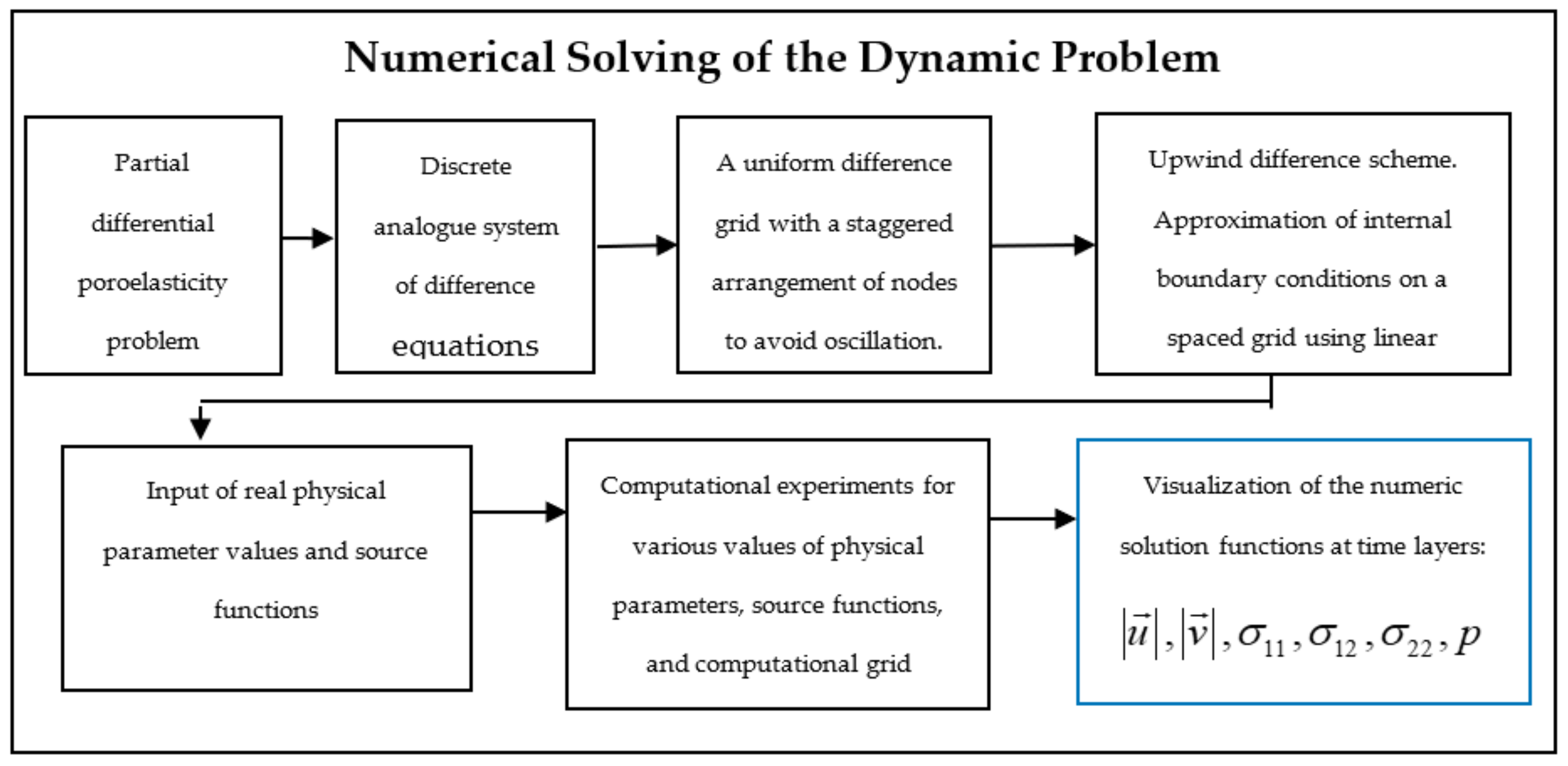
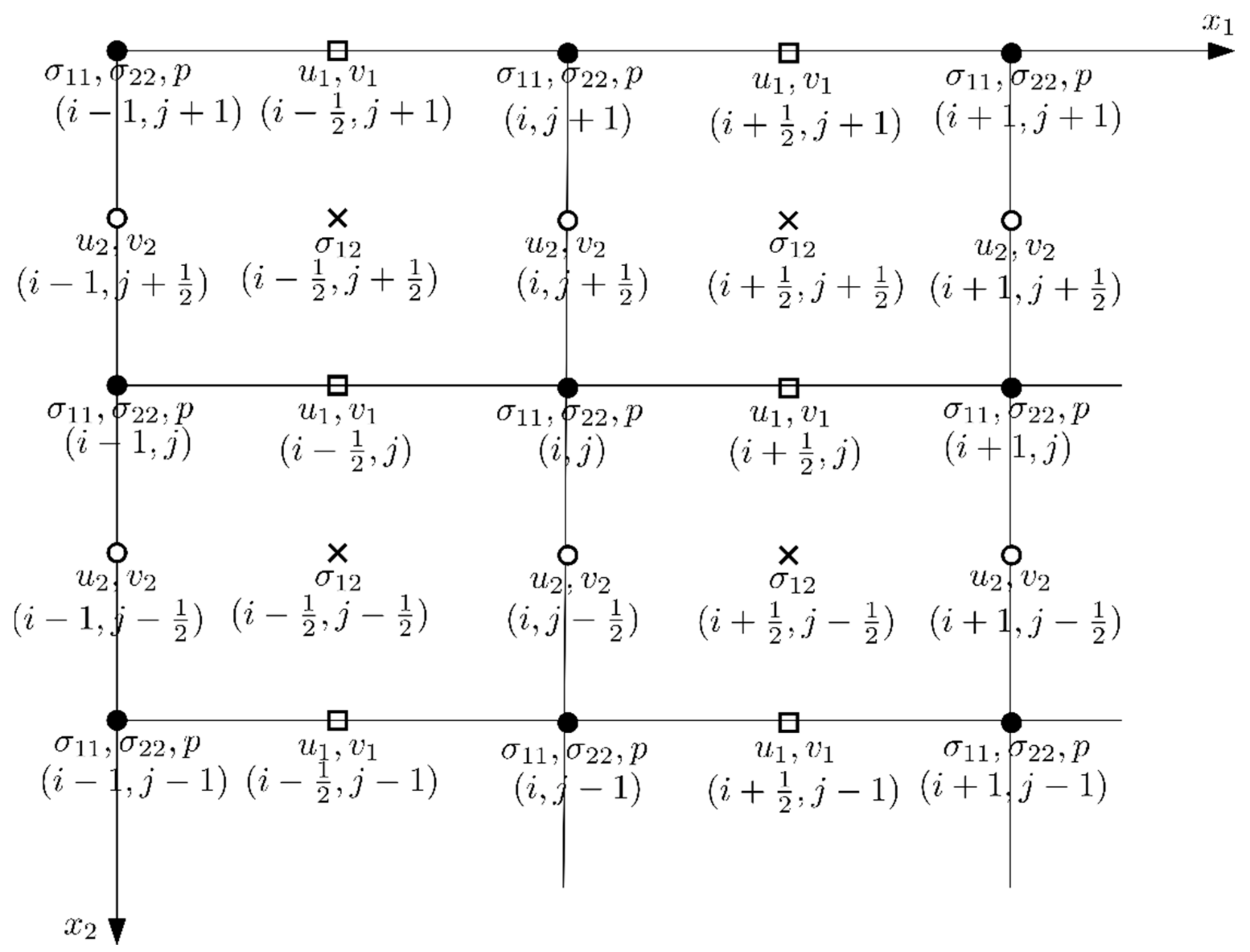
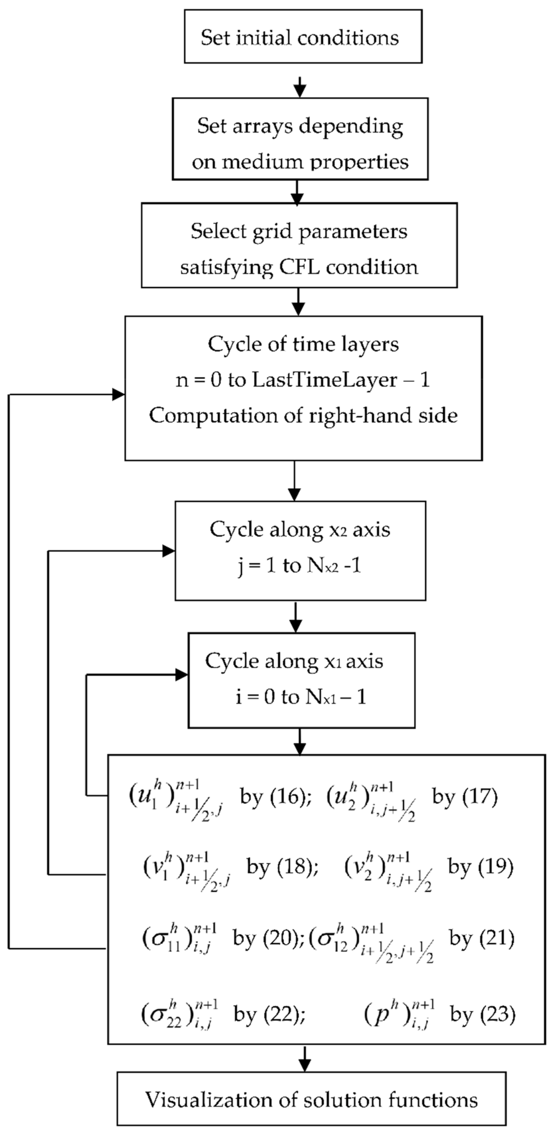
2.2. Discrete Approximation of the Problem

The use of the finite difference method has shown its effectiveness for the numerical solution of the problem stated on the constructed uniform difference grid in the region $Q_T=\left[0,T\right]\times \mathsf{\Omega }\hspace{0.17em}$, where $\mathsf{\Omega }=\left[0,R\right]\times \left[0,L\right]\hspace{0.17em}$ is specified with a staggered arrangement of nodes.

Let us introduce the following notation for such a uniform difference grid:

$$\omega ={\omega }_{\tau }\times {\omega }_h, {\omega }_h={\omega }_h^{\left(1\right)}\times {\omega }_h^{\left(2\right)},\hspace{0.17em}$$

$${\omega }_{\tau }=\left\{t^n=n\tau , n=0,1,\dots ,N_t, N_t\tau =T\right\},\hspace{0.17em}$$

$${\omega }_h^{\left(1\right)}=\left\{x_{1,i}=i{h}_1, i=0,1,\dots ,N_1, N_1{h}_1=R\right\},\hspace{0.17em}$$

$${\omega }_h^{\left(2\right)}=\left\{x_{2,j}=j{h}_2, j=0,1,\dots ,N_2, N_2{h}_2=L\right\}\hspace{0.17em}$$

with a staggered arrangement of nodes shown in Figure 2.

A similar grid was used in [18] to avoid the appearance of oscillations in the solution functions when using central differences on an unstaggered grid. We chose the location of the nodes on the distributed grid in such a way that the longitudinal components of the velocity vectors $\overrightarrow{u}$ and $\overrightarrow{v}$ are determined by the direction of the variable $x_1\hspace{0.17em}$, i.e., $u_1\hspace{0.17em}$ and $\overrightarrow{v}$ are defined at the nodes $\left(i+1/2,j\right)$, and the transverse components $u_2$ and $v_2$ of the indicated vectors are determined in the direction of the variable $x_2\hspace{0.17em}$, i.e., in nodes $\left(i,j+1/2\right)$, the diagonal components of ${\sigma }_{11}\hspace{0.17em}$, ${\sigma }_{22}\hspace{0.17em}$ the stress tensor and pressure are in nodes $\left(i,j\right)\hspace{0.17em}$, the off-diagonal component $\hspace{0.17em}{\sigma }_{12}\hspace{0.17em}$ is in nodes $\left(i+1/2,j+1/2\right)$.

Due to the presence of numerous indices, we introduce the following designations for the desired grid functions with the same letters as in the differential problem (7)–(14), but with the addition of a superscript $h\hspace{0.17em},$ as well as subscripts and superscripts denoting node numbers:

$${\left(u_1^h\right)}_{i,j}^n=u_1\left(i{h}_1,j{h}_2,\tau \hspace{0.17em}n\right),\hspace{0.17em}{\left(u_2^h\right)}_{i,j}^n=u_2\left(i{h}_1,j{h}_2,\tau \hspace{0.17em}n\right),\hspace{0.17em}$$

$${\left(v_1^h\right)}_{i,j}^n=v_1\left(i{h}_1,j{h}_2,\tau \hspace{0.17em}n\right),\hspace{0.17em}{\left(v_2^h\right)}_{i,j}^n=v_2\left(i{h}_1,j{h}_2,\tau \hspace{0.17em}n\right),\hspace{0.17em}$$

$${\left({\sigma }_{11}^h\right)}_{i,j}^n={\sigma }_{11}\left(i{h}_1,j{h}_2,\tau \hspace{0.17em}n\right),\hspace{0.17em}{\left({\sigma }_{12}^h\right)}_{i,j}^n={\sigma }_{12}\left(i{h}_1,j{h}_2,\tau \hspace{0.17em}n\right),\hspace{0.17em}$$

$${\left({\sigma }_{22}^h\right)}_{i,j}^n={\sigma }_{22}\left(i{h}_1,j{h}_2,\tau \hspace{0.17em}n\right),\hspace{0.17em}{\left(p^h\right)}_{i,j}^n=p\left(i{h}_1,j{h}_2,\tau \hspace{0.17em}n\right),\hspace{0.17em}$$

It is assumed that the entire region $\mathsf{\Omega }\hspace{0.17em}=\left[0,R\right]\times \left[0,L\right]$ consists only of a porous medium, where $0<L\hspace{0.17em}$ and $L=N{h}_2\hspace{0.17em}$. Denote by ${\omega }_h\hspace{0.17em}$ the set of nodes of the difference grid, that is:

$${\omega }_h=\left\{\left(x_{1,i},x_{2,j}\right)\in {\omega }_h:\hspace{0.17em}i=0,1,\dots ,N_1, j=0,1,\dots ,N_2\right\}.$$

Let us assign the following explicit difference scheme on a difference grid $\omega \hspace{0.17em}$ to the differential problem:

$$\begin{gathered} \frac{{\left(u_1^h\right)}_{i+\frac{1}{2},j}^{n+1}-{\left(u_1^h\right)}_{i+\frac{1}{2},j}^n}{\tau }+\frac{1}{{\rho }_s}\left(\frac{{\left({\sigma }_{11}^h\right)}_{i+1,j}^n-{\left({\sigma }_{11}^h\right)}_{i,j}^n}{h_1}+\frac{{\left({\sigma }_{12}^h\right)}_{i+\frac{1}{2},j+\frac{1}{2}}^n-{\left({\sigma }_{12}^h\right)}_{i+\frac{1}{2},j-\frac{1}{2}}^n}{h_2}\right)+ \\ \frac{1}{{\rho }_0}\frac{{\left(p^h\right)}_{i+1,j}^n-{\left(p^h\right)}_{i,j}^n}{h_1}={\left(F_1^h\right)}_{i+\frac{1}{2},j}^{n+\frac{1}{2}}, \end{gathered}$$

(16)

$$\begin{gathered} \frac{{\left(u_2^h\right)}_{i,j+\frac{1}{2}}^{n+1}-{\left(u_2^h\right)}_{i,j+\frac{1}{2}}^n}{\tau }+\frac{1}{{\rho }_s}\left(\frac{{\left({\sigma }_{12}^h\right)}_{i+\frac{1}{2},j+\frac{1}{2}}^n-{\left({\sigma }_{12}^h\right)}_{i-\frac{1}{2},j+\frac{1}{2}}^n}{h_1}+\right. \\ \left.\frac{{\left({\sigma }_{22}^h\right)}_{i,j+1}^n-{\left({\sigma }_{22}^h\right)}_{i,j}^n}{h_2}\right)+\frac{1}{{\rho }_0}\frac{{\left(p^h\right)}_{i,j+1}^n-{\left(p^h\right)}_{i,j}^n}{h_2}={\left(F_2^h\right)}_{i,j+\frac{1}{2}}^{n+\frac{1}{2}} \end{gathered}$$

(17)

$$\frac{{\left(v_1^h\right)}_{i+\frac{1}{2},j}^{n+1}-{\left(v_1^h\right)}_{i+\frac{1}{2},j}^n}{\tau }+\frac{1}{{\rho }_0}\frac{{\left(p^h\right)}_{i+1,j}^n-{\left(p^h\right)}_{i,j}^n}{h_1}={\left(F_1^h\right)}_{i+\frac{1}{2},j}^{n+\frac{1}{2}},$$

(18)

$$\frac{{\left(v_2^h\right)}_{i,j+\frac{1}{2}}^{n+1}-{\left(v_2^h\right)}_{i,j+\frac{1}{2}}^n}{\tau }+\frac{1}{{\rho }_0}\frac{{\left(p^h\right)}_{i,j+1}^n-{\left(p^h\right)}_{i,j}^n}{h_2}={\left(F_2^h\right)}_{i,j+\frac{1}{2}}^{n+\frac{1}{2}},$$

(19)

$$\begin{gathered} \frac{{\left({\sigma }_{11}^h\right)}_{i,j}^{n+1}-{\left({\sigma }_{11}^h\right)}_{i,j}^n}{\tau }+{\beta }_1\frac{{\left(u_1^h\right)}_{i+\frac{1}{2},j}^n-{\left(u_1^h\right)}_{i-\frac{1}{2},j}^n}{h_1}+{\beta }_2\frac{{\left(u_2^h\right)}_{i,j+\frac{1}{2}}^n-{\left(u_2^h\right)}_{i,j-\frac{1}{2}}^n}{h_2}- \\ \frac{{\rho }_s}{{\rho }_0}K\left(\frac{{\left(v_1^h\right)}_{i+\frac{1}{2},j}^n-{\left(v_1^h\right)}_{i-\frac{1}{2},j}^n}{h_1}+\frac{{\left(v_2^h\right)}_{i,j+\frac{1}{2}}^n-{\left(v_2^h\right)}_{i,j-\frac{1}{2}}^n}{h_2}\right)=0, \end{gathered}$$

(20)

$$\frac{{\left({\sigma }_{12}^h\right)}_{i+\frac{1}{2},j+\frac{1}{2}}^{n+1}-{\left({\sigma }_{12}^h\right)}_{i+\frac{1}{2},j+\frac{1}{2}}^n}{\tau }+\mu \left(\frac{{\left(u_1^h\right)}_{i+\frac{1}{2},j+1}^n-{\left(u_1^h\right)}_{i+\frac{1}{2},j}^n}{h_2}+\frac{{\left(u_2^h\right)}_{i+1,j+\frac{1}{2}}^n-{\left(u_2^h\right)}_{i,j+\frac{1}{2}}^n}{h_1}\right)=0$$

(21)

$$\begin{gathered} \frac{{\left({\sigma }_{22}^h\right)}_{i,j}^{n+1}-{\left({\sigma }_{22}^h\right)}_{i,j}^n}{\tau }+{\beta }_2\frac{{\left(u_1^h\right)}_{i+\frac{1}{2},j}^n-{\left(u_1^h\right)}_{i-\frac{1}{2},j}^n}{h_1}+{\beta }_1\frac{{\left(u_2^h\right)}_{i,j+\frac{1}{2}}^n-{\left(u_2^h\right)}_{i,j-\frac{1}{2}}^n}{h_2}- \\ \frac{{\rho }_s}{{\rho }_0}K\left(\frac{{\left(v_1^h\right)}_{i+\frac{1}{2},j}^n-{\left(v_1^h\right)}_{i-\frac{1}{2},j}^n}{h_1}+\frac{{\left(v_2^h\right)}_{i,j+\frac{1}{2}}^n-{\left(v_2^h\right)}_{i,j-\frac{1}{2}}^n}{h_2}\right)=0, \end{gathered}$$

(22)

$$\begin{gathered} \frac{{\left(p^h\right)}_{i,j}^{n+1}-{\left(p^h\right)}_{i,j}^n}{\tau }+{\beta }_3\left(\frac{{\left(u_1^h\right)}_{i+\frac{1}{2},j}^n-{\left(u_1^h\right)}_{i-\frac{1}{2},j}^n}{h_1}+\frac{{\left(u_2^h\right)}_{i,j+\frac{1}{2}}^n-{\left(u_2^h\right)}_{i,j-\frac{1}{2}}^n}{h_2}\right)+ \\ \frac{{\rho }_l}{{\rho }_0}\alpha \left(\frac{{\left(v_1^h\right)}_{i+\frac{1}{2},j}^n-{\left(v_1^h\right)}_{i-\frac{1}{2},j}^n}{h_1}+\frac{{\left(v_2^h\right)}_{i,j+\frac{1}{2}}^n-{\left(v_2^h\right)}_{i,j-\frac{1}{2}}^n}{h_2}\right)=0, \end{gathered}$$

(23)

where coefficients ${\beta }_i$, are calculated by the following formulas:

$${\beta }_1=\frac{{\rho }_s}{{\rho }_0}K+\frac{4}{3}\mu , {\beta }_2=\frac{{\rho }_s}{{\rho }_0}K-\frac{2}{3}\mu , {\beta }_3=\frac{{\rho }_s}{{\rho }_0}\alpha -K.$$

We define an algorithm for the numerical solution of the problem as follows. Let the values of the grid functions ${\left(u_1^h\right)}_{i+\frac{1}{2},j}^n\hspace{0.17em},$${\left(u_2^h\right)}_{i,j+\frac{1}{2}}^n\hspace{0.17em},$${\left(v_1^h\right)}_{i+\frac{1}{2},j}^n\hspace{0.17em},$${\left(v_2^h\right)}_{i,j+\frac{1}{2}}^n\hspace{0.17em},$${\left({\sigma }_{11}^h\right)}_{i,j}^n\hspace{0.17em},$${\left({\sigma }_{12}^h\right)}_{i+\frac{1}{2},j+\frac{1}{2}}^n\hspace{0.17em},$${\left({\sigma }_{22}^h\right)}_{i,j}^n\hspace{0.17em},$${\left(p^h\right)}_{i,j}^n\hspace{0.17em}$ on the $n\hspace{0.17em}$-th time layer be known. Then the transition to the $\left(n+1\right)\hspace{0.17em}$-th time layer is carried out according to explicit Formulas (16)–(23), and due to the boundary conditions, the calculation of grid functions ${\sigma }_{12}^h\hspace{0.17em},$${\sigma }_{22}^h$, and $p^h\hspace{0.17em}$ according to Equations (21)–(23) starts from the lower left corner of the computational grid, and calculation of grid functions $u_1^h\hspace{0.17em}$, $u_2^h\hspace{0.17em}$, and $v_2^h\hspace{0.17em}$ by Equations (16)–(19) from the upper right corner. The algorithm of numerical solving of the grid functions is shown on Figure 3.

3. Results

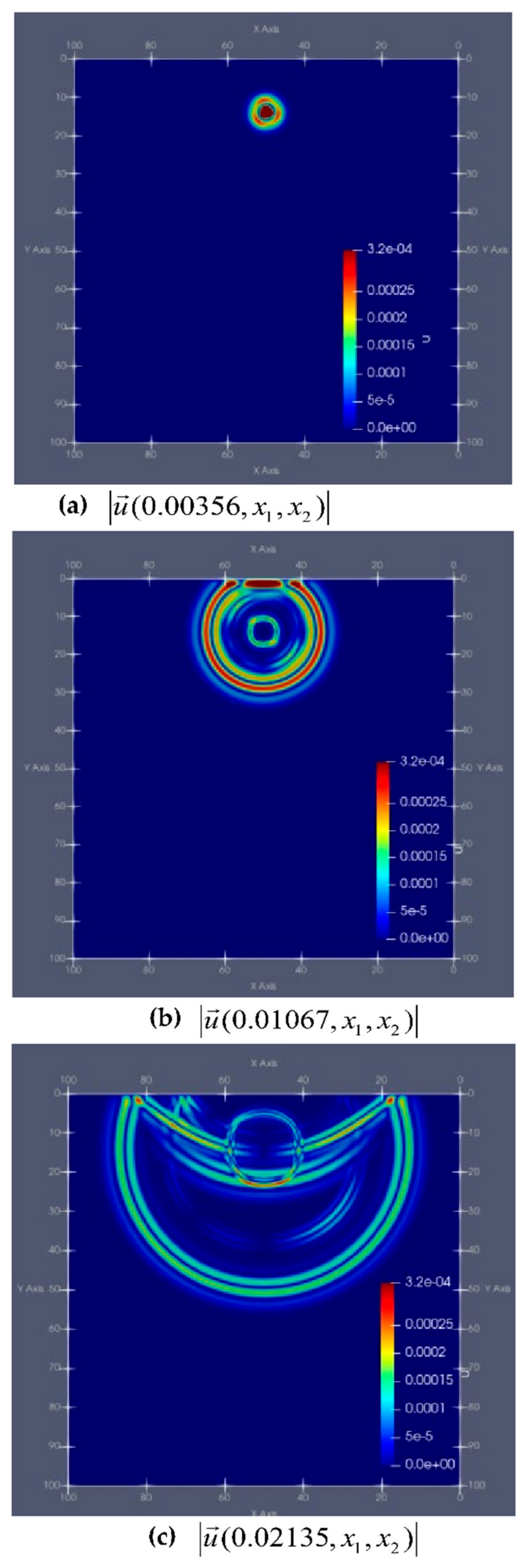
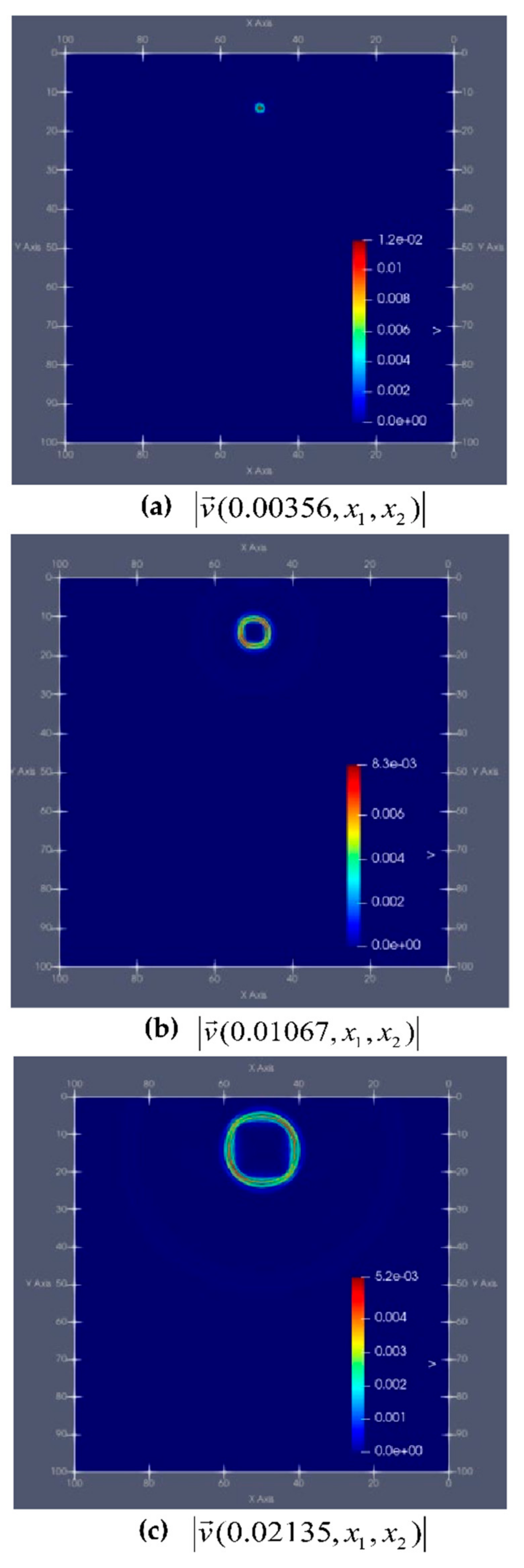
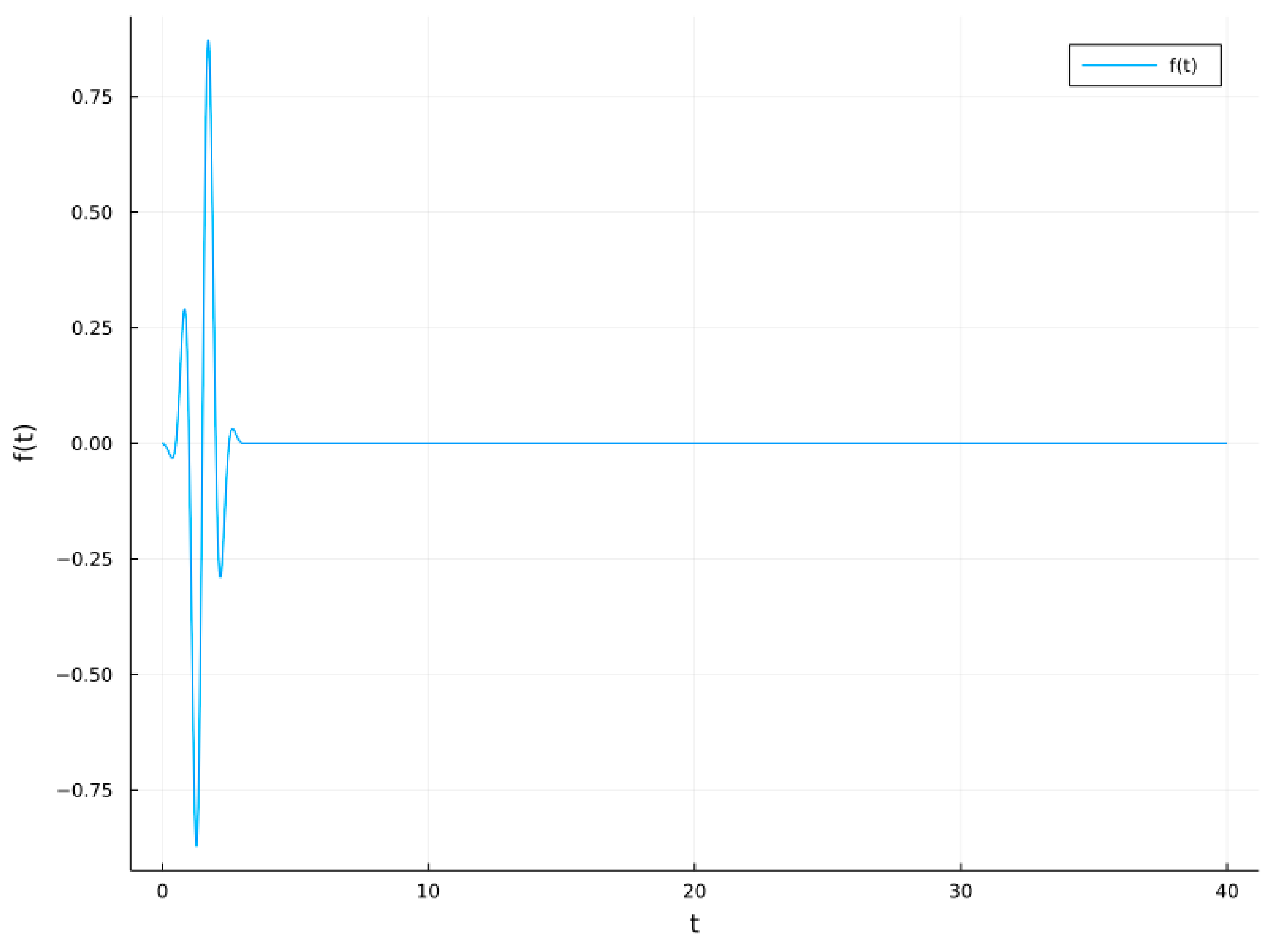
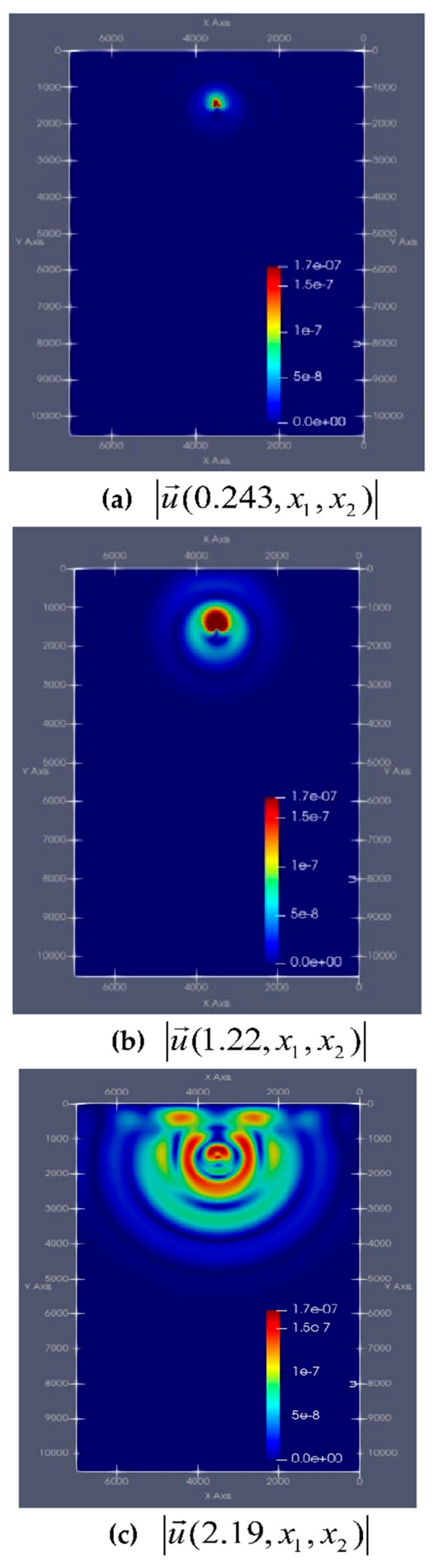
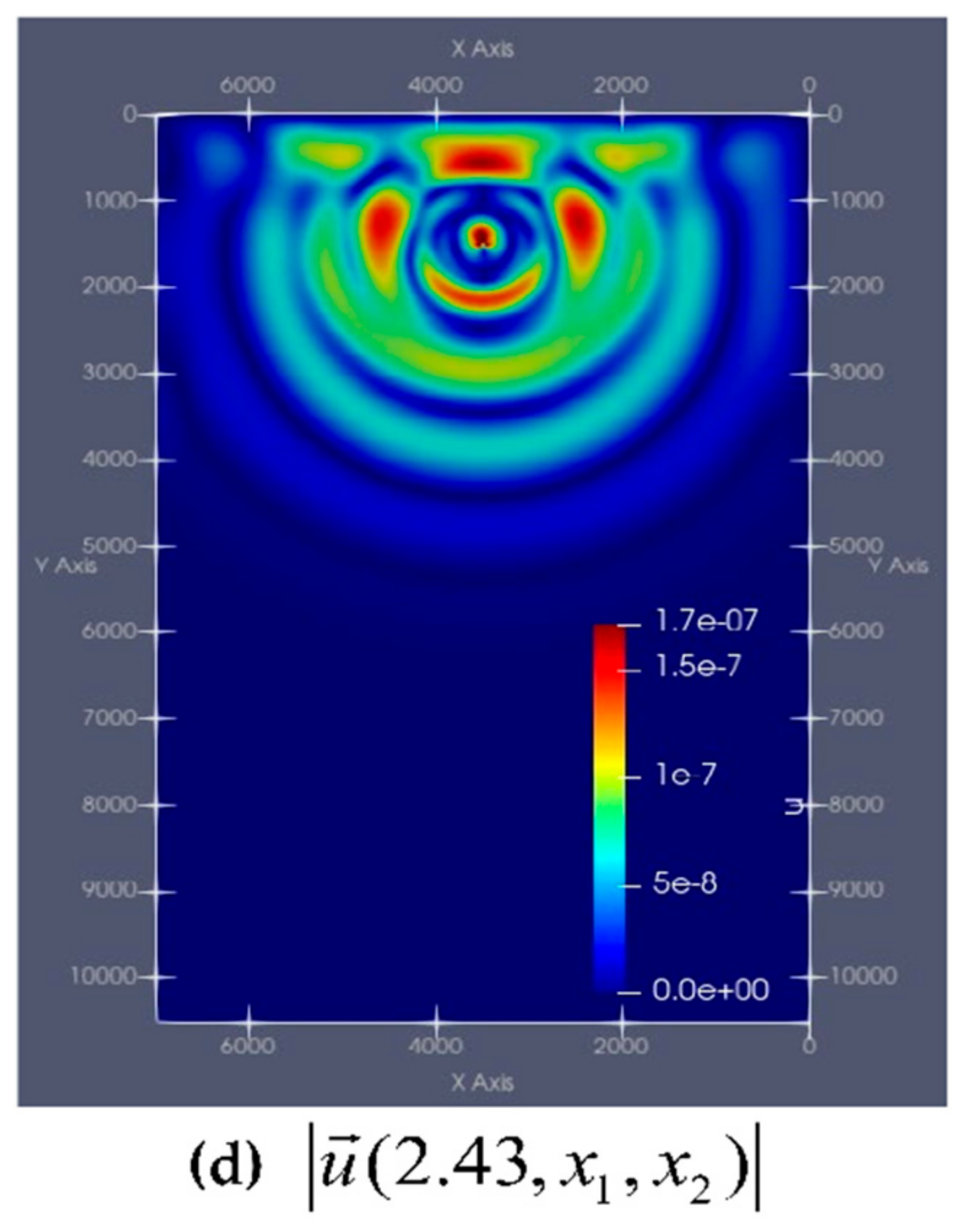
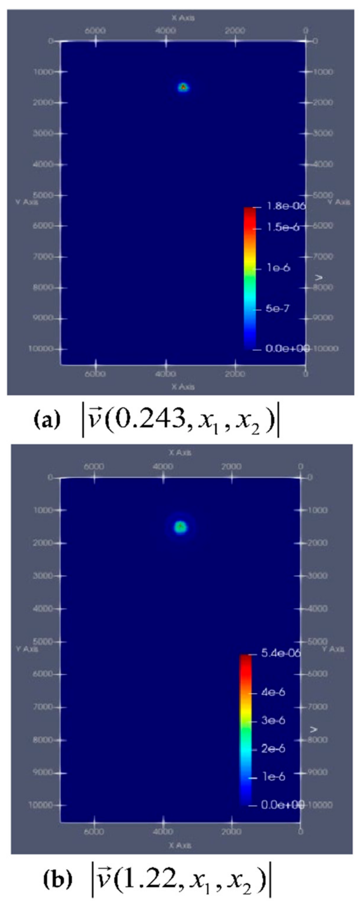
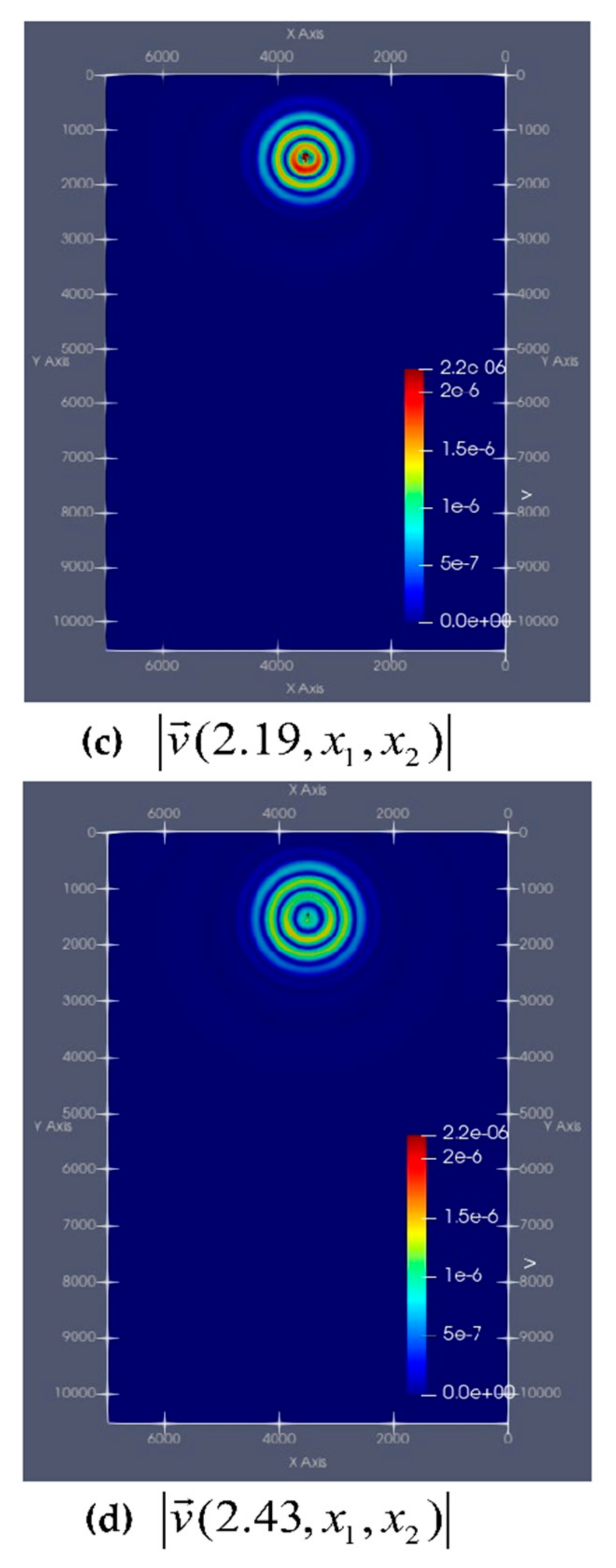
3.1. Computational Experiments

According to the proposed algorithm, two computational experiments were performed, simulating the propagation of seismic wave fields in a two-dimensional elastic porous medium filled with a viscous fluid. The medium is homogeneous and isotropic, the properties of its constituent materials are characterized by the velocities of two longitudinal $c_{p_1}$, $\hspace{0.17em}{c}_{p_2}$ and one transverse sound $c_s$ waves propagating in it. We define a two-dimensional square-shaped region $x\in \mathsf{\Omega }$ with a side of 100 m, in which zero initial conditions and boundary conditions are specified on the left boundary for three functions ${\sigma }_{12}^h\hspace{0.17em},$${\sigma }_{22}^h$, and $p^h\hspace{0.17em}$, and on the right boundary for functions $u_1^h\hspace{0.17em}$, $u_2^h\hspace{0.17em}$, and $v_2^h\hspace{0.17em}$ for various parameter values and a function describing a seismic wavelet.

The program code for the implementation of the algorithm was developed using the new high-performance programming language Julia (free of charge and freely distributed under the MIT license).

The calculations were implemented using parallel computing on a computer with the technical characteristics shown in

Table 1. Hardware description.

Description	Technical Characteristics
Processor	16-core AMD Ryzen 9 3950X
Clock speed/Frequency	3.5 GHz (Matisse)
RAM	64 GB

:

The use of an explicit computational scheme, which contain the cyclic sections, enables the software to create parallelized algorithm and allows the efficient use of the computational resources.

The dynamic visualization of the computational experiments results presented in this paper was performed using ParaView software package.

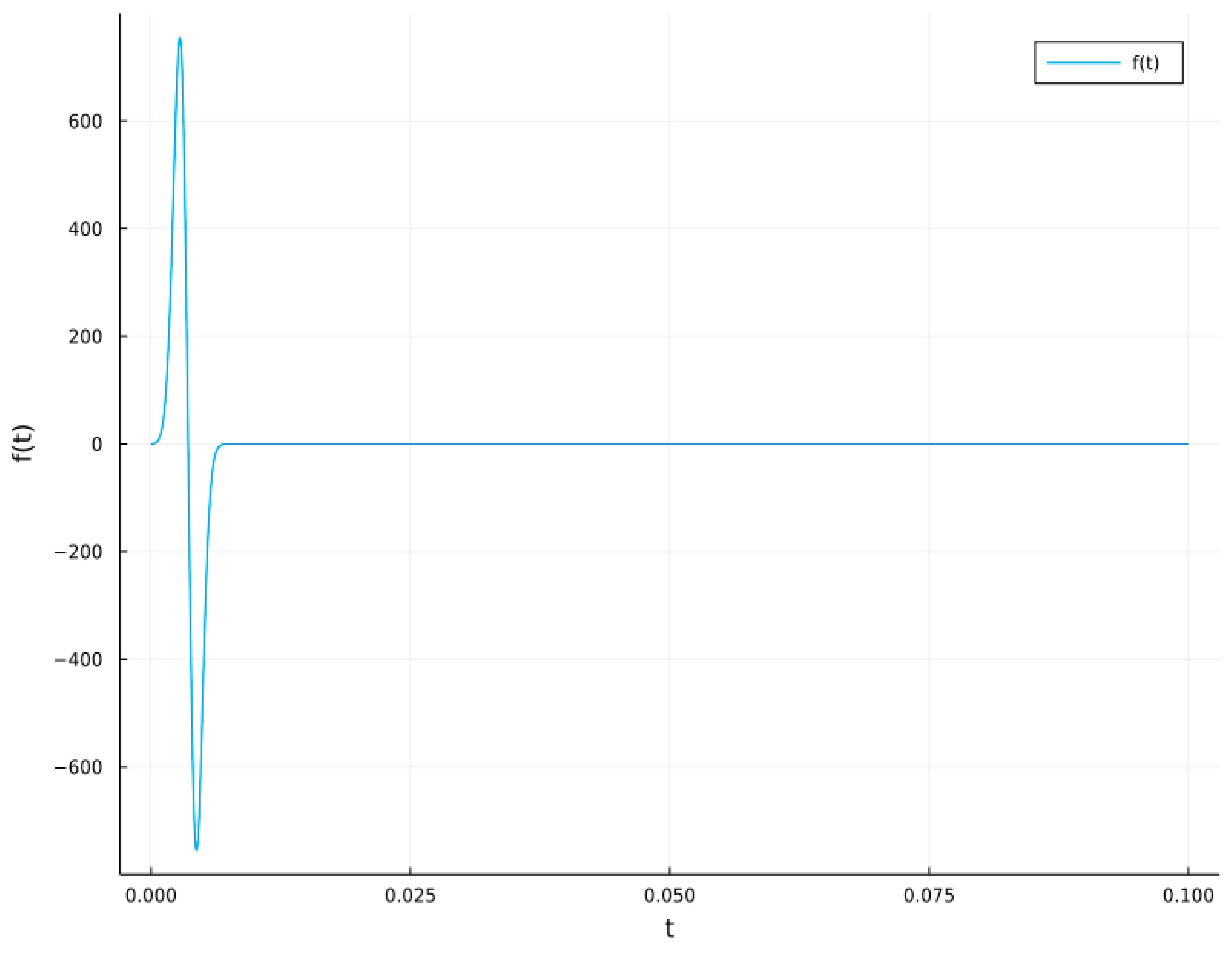
3.1.1. First Computational Experiment

The real input data for physical parameters in the first computational experiment of the problem are taken from [19] and are shown in

Table 2. Input physical parameters and grid characteristics in the first computational experiment.

##	Name of the Input Physical and Grid Parameter	Notation	Value	Units
1	Matrix physical density	${\rho }_s^f$	1.5	${\mathrm{g}/\mathrm{cm}}^3$
2	Fluid physical density	${\rho }_l^f$	1	${\mathrm{g}/\mathrm{cm}}^3$
3	Fast longitudinal wave velocity	$c_{p_1}$	$2000$	$\mathrm{m}/\mathrm{s}$
4	Slow longitudinal wave velocity	$c_{p_2}$	$450$	$\mathrm{m}/\mathrm{s}$
5	Transverse wave velocity	$c_s$	$1400$	$\mathrm{m}/\mathrm{s}$
6	Porosity	$d_0$	$0.2$
7	Integration area along $x_1$ axis	$R$	100	$\mathrm{m}$
8	Integration area along $x_2$-axis	$L$	100	$\mathrm{m}$
9	Number of nodes along $x_1$ axis	$N_1$	$400$
10	$\mathrm{Number} \mathrm{of} \mathrm{nodes} \mathrm{along} x_2$ axis	$N_2$	$400$
11	Number of time layers	$N_t$	${10}^5$
12	$\mathrm{Step} \mathrm{along} \mathrm{axis} x_1$	$h_1$	$\frac{R}{N_1}=\frac{100}{400}=0.25$	M
13	$\mathrm{Step} \mathrm{along} \mathrm{axis} x_2$	$h_2$	$\frac{L}{N_2}=\frac{100}{400}=0.25$	m
14	Step in time	$\tau$	$\frac{9\cdot {10}^{-5}\cdot h_1}{20\sqrt{10}}\approx 3.5575\cdot {10}^{-7}$	s
15	The signal propagation time	$T$	$0.02135$	s
16	Dimensionless source Parameter	$\tilde{\gamma }$	4
17	The source central Frequency	$f_0$	1	Hz
18	Source duration	$t_0$	1	S

:

The source function $F\left(t,x_1,x_2\right)=(F_1\left(t,x_1,x_2\right),F_2\left(t,x_1,x_2\right))$ is described by the following formulas:

$$F_1\left(t,x_1,x_2\right)=f\left(t\right)\frac{\partial \delta \left(x-x_0\right)}{\partial x_1}\delta \left(x-x_0\right),$$

$$F_2\left(t,x_1,x_2\right)=f\left(t\right)\delta \left(x-x_0\right)\frac{\partial \delta \left(x-x_0\right)}{\partial x_2},$$

where the momentum function is described by the formula:

$$f(t)=\left\{\begin{array}{l}-2{\pi }^2{f}_0^2\cdot (t-t_0)\exp (-{\pi }^2{f}_0^2\cdot {(t-t_0)}^2), t\le 2t_0,\\ 0, t>2t_0\end{array}\right.$$

$$x_0=(x_1^0,\hspace{0.17em}\hspace{0.17em}{x}_2^0)=(50,\hspace{0.17em}\hspace{0.17em}14).$$

The graph of the function $f(t)$ is shown in Figure 4.

In this case, the two-dimensional delta function $\delta \left(x\right)$, $x=\left(x_1,x_2\right)$ is approximated using the “hat” function of the form:

$$\delta \left(x\right)\approx {\Delta }_1\left(x\right)=\left\{\begin{array}{ll}exp\left(-\frac{{\epsilon }^2}{{\epsilon }^2-{\left|x\right|}^2}\right),\hfill & \left|x\right|<\epsilon ,\hfill \\ 0,\hfill & \left|x\right|\ge \epsilon ,\hfill \end{array}\right.$$

where $\epsilon \to 0$ is the parameter. The partial derivative of this function with respect to the variable $x_k$, $\left(k=1,2\right)$ has the form:

$$\frac{\partial }{\partial x_k}{\Delta }_1\left(x\right)=\left\{\begin{array}{ll}-\frac{2{\epsilon }^2{x}_k}{{\left({\epsilon }^2-{\left|x\right|}^2\right)}^2}exp\left(-\frac{{\epsilon }^2}{{\epsilon }^2-{\left|x\right|}^2}\right),\hfill & \left|x\right|<\epsilon ,\hfill \\ 0,\hfill & \left|x\right|\ge \epsilon .\hfill \end{array}\right.$$

Visualization of the results of computational experiments is shown in Figure 5 and Figure 6.

Figure 5 and Figure 6 show the dynamics of the modulus of the vectors $\left|\overrightarrow{u}\right|=\sqrt{u_1^2+u_2^2}$ and $\left|\overrightarrow{v}\right|=\sqrt{v_1^2+v_2^2}$ from time $t=0.00356$ s. to $t=0.02135$ s. with certain time intervals. The computational process in this experiment took 34 min.

On the dynamic graphs on Figure 5 and Figure 6 we can observe that the velocity in a solid phase change faster in time that in a liquid phase, which is in agreement with the observed experimental data.

The seismograms of components $u_1(x_2,t)$ and $u_2(x_2,t)$ along the traces going through the source point are shown in Figure 7 and Figure 8, respectively.

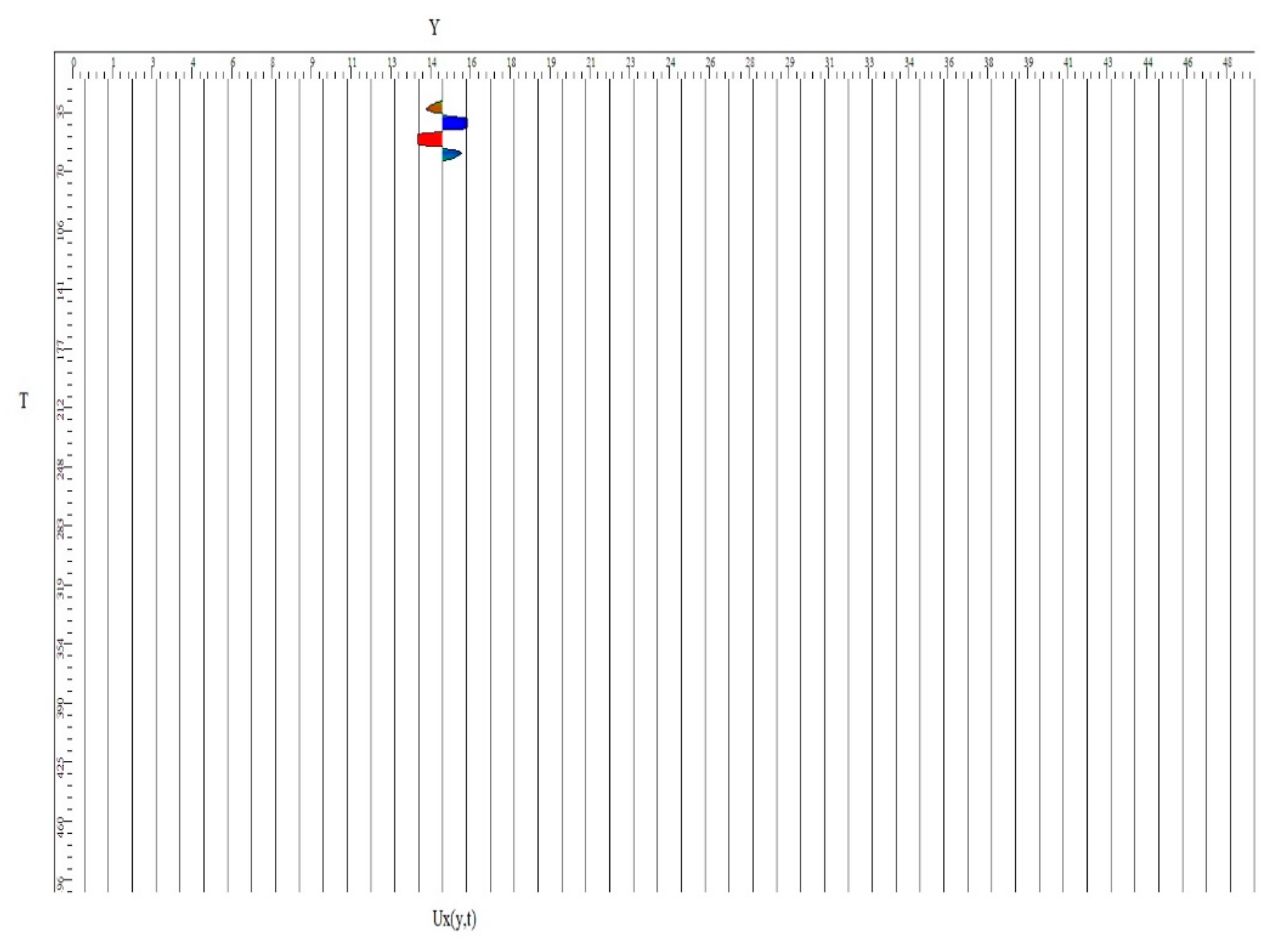
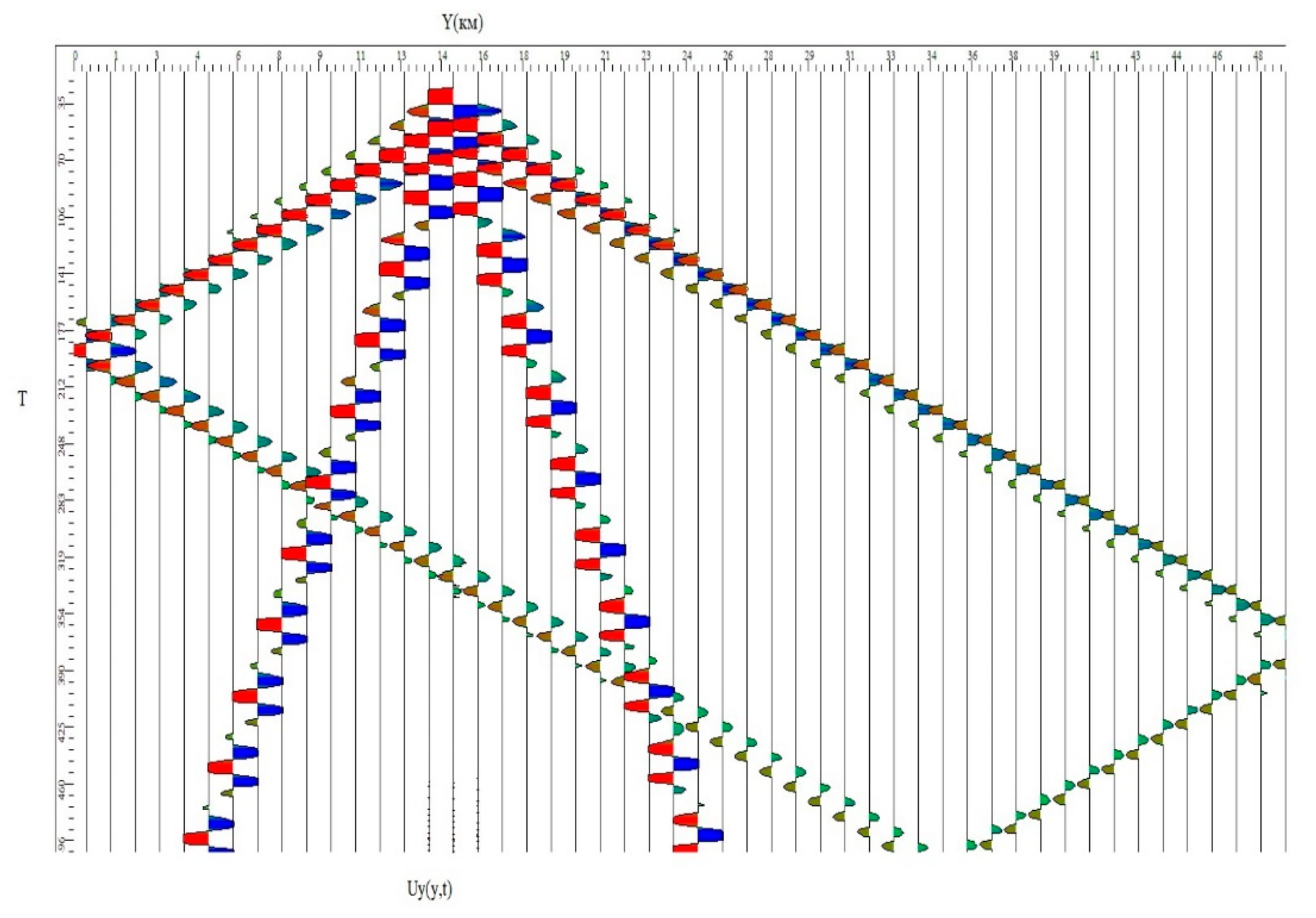
3.1.2. The Second Computational Experiment

In the second computational experiment, the different set of values of physical parameters shown in

Table 3. Input physical parameters and grid characteristics in the second computational experiment.

##	Name of the Input Physical and Grid Parameter	Notation	Value	Units
1	Matrix physical density	${\rho }_s^f$	1.5	${\mathrm{g}/\mathrm{cm}}^3$
2	Fluid physical density	${\rho }_l^f$	1	${\mathrm{g}/\mathrm{cm}}^3$
3	Fast longitudinal wave velocity	$c_{p_1}$	$2100$	$\mathrm{m}/\mathrm{s}$
4	Slow longitudinal wave velocity	$c_{p_2}$	$500$	$\mathrm{m}/\mathrm{s}$
5	Transverse wave velocity	$c_s$	$1400$	$\mathrm{m}/\mathrm{s}$
6	Porosity	$d_0$	$0.2$
7	$\mathrm{Integration} \mathrm{area} \mathrm{along} x_1$ axis	$R$	$7000$	$\mathrm{m}$
8	$\mathrm{Integration} \mathrm{area} \mathrm{along} x_2$-axis	$L$	10500	$\mathrm{m}$
9	$\mathrm{Number} \mathrm{of} \mathrm{nodes} \mathrm{along} x_1$ axis	$N_1$	$400$
10	$\mathrm{Number} \mathrm{of} \mathrm{nodes} \mathrm{along} x_2$ axis	$N_2$	$400$
11	Number of time layers	$N_t$	$5\cdot {10}^5$
12	$\mathrm{Steps} \mathrm{along} \mathrm{axis}{x}_1$	$h_1$	$\frac{R}{N_1}=\frac{100}{400}=0.25$	m
13	$\mathrm{Steps} \mathrm{along} \mathrm{axis} x_2$	$h_2$	$\frac{L}{N_2}=\frac{100}{400}=0.25$	m
14	Step in time	$\tau$	$\frac{9\cdot {10}^{-5}{h}_1}{\sqrt{4200}}\approx 2.4303\cdot {10}^{-5}$	s
15	The signal propagation time	$T$	2.43	s
16	Dimensionless source parameter	$\tilde{\gamma }$	4
17	The source central frequency	$f_0$	1	Hz
18	Source duration	$t_0$	1	s

and the form of the source function describing the seismic pulse of the problem are taken from [20]:

Source function $F\left(t,x_1,x_2\right)=(F_1\left(t,x_1,x_2\right),F_2\left(t,x_1,x_2\right))$ is described by the following formulas:

$$\begin{gathered} F_1\left(t,x_1,x_2\right)=f\left(t\right)\frac{\partial \delta \left(x-x_0\right)}{\partial x_1}\delta \left(x-x_0\right), \\ {F}_2\left(t,x_1,x_2\right)=f\left(t\right)\delta \left(x-x_0\right)\frac{\partial \delta \left(x-x_0\right)}{\partial x_2}, \end{gathered}$$

where $f(t)=\exp \left(-\frac{{(2\pi f_0\cdot (t-t_0))}^2}{{\gamma }^2}\right)\sin \left(2\pi f_0\cdot (t-t_0)\right)$ (Puzyrev impulse) $x_0=\left(3500\hspace{0.17em}\hspace{0.17em}m,\hspace{0.17em}\hspace{0.17em}1500\hspace{0.17em}\hspace{0.17em}m\right)$—source coordinates.

The delta function $\delta \left(x-x_0\right)$ and its partial derivatives are approximated in a similar way as in the first computational experiment using the “hat” function.

The graph of the impulse function $f(t)$ is shown in Figure 9.

Figure 10 and Figure 11 show the dynamics of the modulus of the vectors $\left|\overrightarrow{u}\right|=\sqrt{u_1^2+u_2^2}$ and $\left|\overrightarrow{v}\right|=\sqrt{v_1^2+v_2^2}$ from point of time $t=0.243$ s to $t=2.43$ s at certain intervals.

The seismograms of components $u_1(x_2,t)$ and $u_2(x_2,t)$ along the traces going through the source point look similar to the seismograms shown in the first computational experiment.

The program code implementing parallel computing is developed in the high-performance Julia programming language. The possibility of using the approach is demonstrated by the example of solving the problem of propagation of seismic waves from a source located in the formation. Computational experiments based on realistic data from oil reservoirs have been implemented and dynamic visualization of solutions consistent with the first waves entry times has been obtained.

4. Discussion

Thus, an original algorithm for the numerical solution of the initial-boundary value problem for the poroelasticity system is presented. This problem models the propagation of seismic waves in a poroelastic medium saturated with a fluid, characterized by such physical parameters as the propagation velocities of longitudinal and transverse waves, the physical density of the medium materials, and porosity. This approach has important industrial applications. Modeling of seismic waves propagation is instrumental for seismic surveys as the most reliable geophysical technique used to identify oil and gas prospects in the geologic structures. This paper introduces a new approach to the computer simulation of wave propagation processes in complex multiphase media. The proposed algorithm allows efficient use of parallel computations on computers with multi-core processors. Thanks to improvements in high-performance modern computing systems, the introduction of a new approach to computer simulation technology may play a critical role in the field of data processing and interpretation and in other applications. The use of a staggered grid method enabled us to avoid oscillations of the eight solution functions in a two-dimensional case of the problem. The solution is implemented using an explicit finite difference upwind scheme built on a staggered grid using parallel computing. The continuum filtration approach makes it possible to describe the poroelastic medium with a smaller number of model parameters than in the Frenkel–Biot theory of poroelasticity and with a better agreement with experimental data.

The numerical modeling allows the conduction of numerical experiments with fully controlled input data and thereby reliably verifying hypotheses and formulating criteria for the manifestation of fluid mobility in seismic data. The program code implementing parallel computing is developed in the high-performance Julia programming language. The stability of the proposed scheme is ensured by the satisfaction of the Friedrichs–Courant–Lewy criterion. Computational experiments based on real data from oil reservoirs have been implemented, and dynamic visualization of solutions consistent with the first waves arrival times has been obtained.

This work is mainly aimed at demonstrating the numerical method for solving the stated poroelasticity problem, while the results of the theoretical study of the resolvability conditions and the expression of the analytical solution in explicit form will be the subject of a separate paper.

This investigation presents an algorithm for the numerical solution of an initial-boundary value problem for a system of symmetric partial differential equations of t-hyperbolic type. This will be crucial for research in various areas, such as medicine, chemical engineering, micro and nanofluidics.

5. Patents

The authors are planning to create an easily usable interface allowing implementation of solutions for various input data of physical parameters values and a source function form based on the algorithm described in the article. Once this work is completed, a patent will be obtained resulting from the work reported in this manuscript.

References

1. Carcione, J.M.; Morency, C.; Santos, J.E. Computational poroelasticity—A review. Geophysics 2010, 75, 75A229–75A243. [Google Scholar] [CrossRef]
2. Yang, Q.; Mao, W. Simulation of seismic wave propagation in 2-D poroelastic media using weighted-averaging finite difference stencils in the frequency space domain. Geophys. J. Int. 2017, 208, 148–161. [Google Scholar] [CrossRef]
3. Duclous, R.; Dubroca, B.; Frank, M. A deterministic partial differential equation model for dose calculation in electron radiotherapy. Phys. Med. Biol. 2010, 55, 3843–3857. [Google Scholar] [CrossRef] [PubMed]
4. Loureiro, J.M.; Rodrigues, A. Two solution methods for hyperbolic systems of partial differential equations in chemical engineering. Chem. Eng. Sci. 1991, 46, 3259–3267. [Google Scholar] [CrossRef]
5. Lim, C.Y.; Lim, A.E.; Lam, Y.C. pH change in electroosmotic flow hysteresis. Anal. Chem. 2017, 89, 9394–9399. [Google Scholar] [CrossRef] [PubMed]
6. Lim, A.E.; Lam, Y.C. Vertical Squeezing Route Taylor Flow with Angled Microchannel Junctions. Ind. Eng. Chem. Res. 2021, 60, 14307–14317. [Google Scholar] [CrossRef]
7. Shafiq, A.; Lone, S.A.; Sindhu, T.N.; Al-Mdallal, Q.M.; Rasool, G. Statistical modeling for bioconvective tangent hyperbolic nanofluid towards stretching surface with zero mass flux condition. Sci. Rep. 2021, 11, 13869. [Google Scholar] [CrossRef]
8. Frenkel, I.I. On the theory of seismic and seismoelectrical phenomena in wet soil. Izv. Acad. Sci. USSR Ser. Geogr. Geophys 1944, 8, 133–150. (In Russian) [Google Scholar] [CrossRef]
9. Biot, M.A. Theory of propagation of elastic waves in fluid-saturated porous solids. J. Acoust. Soc. Am. 1956, 28, 168–186. [Google Scholar] [CrossRef]
10. Dorovsky, V.N. Mathematical models of two-velocity media. Part I. Math. Comput. Modeling 1995, 21, 17–28. [Google Scholar] [CrossRef]
11. Dorovsky, V.N.; Perepechko, Y.V. Mathematical models of two-velocity media. Part II. Math. Comput. Modeling 1996, 24, 69–80. [Google Scholar] [CrossRef]
12. Dorovsky, V.N.; Perepechko, Y.V.; Fedorov, A.I. Stoneley waves in the Biot-Jonson and Continuum filtration theories. Russ. Geol. Geophys. 2012, 53, 471–479. [Google Scholar] [CrossRef]
13. Zhu, X.; McMechan, G.A. Numerical simulation of seismic responses of poroelastic reservoirs using Biot theory. Geophysics 1991, 56, 328–339. [Google Scholar] [CrossRef]
14. Zeng, Y.Q.; He, J.Q.; Liu, Q.H. The application of the perfectly matched layer in numerical modeling of wave propagation in poroelastic media. Geophysics 2001, 66, 1258–1266. [Google Scholar] [CrossRef]
15. Philippacopoulos, A.J. Lamb’s problem for fluid-saturated porous media. Bull. Seismol. Soc. Am. 1988, 7, 908–923. [Google Scholar]
16. Miroshnokov, V.V.; Fatianov, A.G. Semi-analytical method for calculating wave fields in layered porous media. Math. Modeling Geophys. 1993, 1, 27–57. [Google Scholar]
17. Dai, N.; Vafidis, A.; Kanasewich, E.R. Wave propagation in heterogeneous, porous media: A velocity-stress, finite-difference method. Geophysics 1995, 60, 327–340. [Google Scholar] [CrossRef]
18. Dorovsky, V.N.; Perepechko, Y.V.; Romenskiy, E.I. Wave processes in saturated elastically deformable medium. Phys. Combust. Explos. 1993, 1, 100–111. (In Russian) [Google Scholar]
19. Sorokin, K.E.; Imomnazarov, K.K. Numerical solving of the liner two-dimensional dynamic problem in liquid-filled porous media. J. Sib. Fed. Univ. Math. Phys. 2010, 3, 256–261. (In Russian) [Google Scholar]
20. Berdyshev, A.S.; Imomnazarov, K.K.; Tang, J.-G.; Mikhailov, A. The Laguerre spectral method as applied to the numerical solution of a two-dimensional linear dynamic seismic problem for porous media. Open Comput. Sci. 2016, 6, 208–212. [Google Scholar] [CrossRef]
21. Dorovsky, V.N.; Imomnazarov, K.K. Mathematical model for the movement of a conducting liquid through a conducting porous medium. Math. Comput. Modeling 1994, 20, 91–97. [Google Scholar] [CrossRef]
22. Imomnazarov, K.K.; Imomnazarov, S.K.; Mamatqulov, M.M.; Chernykh, E.G. The fundamental solution of the stationary two-velocity hydrodynamics equation with one pressure. In Bulletin of the Novosibirsk Computing Center; Series: Mathemaical Modeling in Geophysics; NCC Publisher: Novosibirsk, Russia, 2014. [Google Scholar]
23. Meirmanov, A. Atlantis Studies in Differential Equations. In Mathematical Models for Poroelastic Flows; Springer: Berlin, Germany, 2014; Volume 1. [Google Scholar] [CrossRef]
24. Berdyshev, A.S.; Imomnazarov, K.K.; Tang, J.-G.; Tuchieva, S. The symmetric form of poroelasticity dynamic equations in terms of velocities, stresses, and pressure. Open Eng. Former. Cent. Eur. J. Eng. 2016, 6, 322–325. [Google Scholar] [CrossRef]
25. Blokhin, A.M.; Dorovsky, V.N. Mathematical Modeling in the Theory of Multi-Velocity Continuum; Nova Sci: New York, NY, USA, 1995. [Google Scholar]
26. Garipov, T.T. Modeling of hydraulic fracturing in a poroelastic medium. Math. Modeling 2006, 18, 53–69. [Google Scholar]
27. Virieux, J.; Calandra, H.; Plessix, R.E. A review of the spectral, pseudo-spectral, finite-difference and finite-element modelling techniques for geophysical imaging. Geophys. Prospect. 2011, 59, 794–813. [Google Scholar] [CrossRef]
28. Carcione, J.M.; Herman, C.G.; Kroode, P.E. Y2K Review Article: Seismic Modeling. Rev. Lit. Arts Am. 2002, 67, 1304–1325. [Google Scholar]
29. Breus, A.; Favorskaya, A.; Golubev, V.; Kozhemyachenko, A.; Petrov, I. Investigation of Seismic Stability of High-Rising Buildings Using Grid-Characteristic Method. Procedia Comput. Sci. 2019, 154, 305–310. [Google Scholar] [CrossRef]
30. Volkov, K.N. Implementation of a splitting scheme on a staggered grid for calculating unsteady flows of a viscous incompressible fluid. Comput. Methods Program. 2005, 6, 269–282. (In Russian) [Google Scholar]
Figure 1. Flowchart of the numerical solving of the dynamic poroelasticity problem.
Symmetry 14 01516 g001
Figure 2. Grid with a staggerred arrangement of nodes.
Symmetry 14 01516 g002
Figure 3. Flowchart of the numerical solving of the grid functions.
Symmetry 14 01516 g003
Figure 4. Function f ( t ) in the first computational experiment.
Symmetry 14 01516 g004
Figure 5. Graph of the module of the solid phase velocity in the first computational experiment at time intervals: (a) t = 0.00356 s , (b) t = 0.01067 s , (c) t = 0.02135   s .
Symmetry 14 01516 g005
Figure 6. Graph of the module velocity vector of a liquid phase in the first computational experiment at certain time intervals: (a) t = 0.00356   s , (b) t = 0.01067   s , (c) t = 0.02135   s .
Symmetry 14 01516 g006
Figure 7. Seismogram of u 1 ( x 2 , t ) component.
Symmetry 14 01516 g007
Figure 8. Seismogram of u 2 ( x 2 , t ) component.
Symmetry 14 01516 g008
Figure 9. Function f ( t ) in the second computational experiment.
Symmetry 14 01516 g009
Figure 10. Graph of the module velocity of the solid phase u in the second computational experiment at particular time intervals: (a) t = 0.243 s, (b) t = 1.22 s, (c) t = 2.19 s, (d) t = 2.43 s.
Symmetry 14 01516 g010aSymmetry 14 01516 g010b
Figure 11. Graph of the module velocity of the liquid phase in the second computational experiment at particular time intervals: (a) t = 0.243 s, (b) t = 1.22 s, (c) t = 2.19 s, (d) t = 2.43 s.
Symmetry 14 01516 g011aSymmetry 14 01516 g011b