Optimal Plan of Multi-Stress–Strength Reliability Bayesian and Non-Bayesian Methods for the Alpha Power Exponential Model Using Progressive First Failure

Abstract

It is extremely frequent for systems to fail in their demanding operating environments in many real-world contexts. When systems reach their lowest, highest, or both extreme operating conditions, they usually fail to perform their intended functions, which is something that researchers pay little attention to. The goal of this paper is to develop inference for multi-reliability using unit alpha power exponential distributions for stress–strength variables based on the progressive first failure. As a result, the problem of estimating the stress–strength function R, where X, Y, and Z come from three separate alpha power exponential distributions, is addressed in this paper. The conventional methods, such as maximum likelihood for point estimation, Bayesian and asymptotic confidence, boot-p, and boot-t methods for interval estimation, are also examined. Various confidence intervals have been obtained. Monte Carlo simulations and real-world application examples are used to evaluate and compare the performance of the various proposed estimators.

1. Introduction

Systems failing to perform in their harsh working settings is a common occurrence in real-life scenarios. When crossing their lower, upper, or both extreme operating conditions, systems frequently fail to perform their intended roles. Stress–strength reliability, often known as $\mathrm{R}=\mathrm{p}\left(\mathrm{X}<\mathrm{Y}\right)$, has been extensively investigated in the literature. When the applied stress exceeds the system’s strength, a system working under such stress–strength conditions fail to function. Refs. [1,2,3,4,5,6,7,8,9,10,11] are only a few of the significant efforts in this direction. Moreover, the study of stress–strength models has been expanded to multi-component systems, which are systems with several components. Despite the fact that Ref. [12] developed the multi-component stress–strength model decades ago, it has garnered a lot of attention in recent years and has been explored by numerous scholars for both complete and filtered data [13,14,15,16,17]. Stress–strength reliability, $\mathrm{R}=\mathrm{P}(\mathrm{X}<\mathrm{Y})$, has been extensively investigated as a stress–strength model, and the research has also been extended to multi-component systems. However, an equally important practical scenario in which equipment fails in extreme lower and upper working environments receives significantly less attention. When electrical equipment is placed below or above a specified power supply, for example, it will fail. A person’s systolic and diastolic pressure limits should not be exceeded at the same time. There are a plethora of such applications, many of them are straightforward and natural, reflecting sound correlations between diverse real-world events. It is a valuable relationship in a variety of subfields of genetics and psychology, where strength Y should not only be more than stress X, but also less than stress Z. For numerous statistical models, several scholars have examined the estimation of the stress–strength parameter. Refs. [18,19,20] investigated the estimation of $\mathrm{R}=\mathrm{P}(\mathrm{X}<\mathrm{Y}<\mathrm{Z})$ based on independent samples. Ref. [21] obtained the estimation in the stress–strength model with the assumption that a component’s strength lies in an interval and the probability $\mathrm{R}=\mathrm{P}({\mathrm{X}}_1<\mathrm{Y}<{\mathrm{X}}_2),$ where ${\mathrm{X}}_1$ and ${\mathrm{X}}_2$ are random stress variables and $\mathrm{Y}$ is a random strength variable. When $\left({\mathrm{Y}}_1,{\mathrm{Y}}_2,\dots ,{\mathrm{Y}}_{\mathrm{k}}\right)$ are normal random variables, $\mathrm{X}$ is another independent normal random variable, and the estimation of $\mathrm{R}=\mathrm{P}\left[\max \left({\mathrm{Y}}_1,{\mathrm{Y}}_2,\dots ,{\mathrm{Y}}_{\mathrm{k}}\right)<\mathrm{X}\right]$ is considered. Ref. [22] calculated the reliability of a component that was subjected to two separate stresses that were unrelated to the component’s strength. Ref. [23] used a multi-component series stress–strength model to predict system reliability. Using current U-statistics, Ref. [24] proposed a straightforward computation procedure for $\mathrm{P}(\mathrm{X}<\mathrm{Y}<\mathrm{Z})$ and its variance. $\mathrm{P}(\mathrm{X}<\mathrm{Y}<\mathrm{Z})$ was used by Ref. [24] to study the cascade system. Nonparametric statistical inference for $\mathrm{P}(\mathrm{X}<\mathrm{Y}<\mathrm{Z})$ was studied by Ref. [25]. Ref. [26] achieved inference of $\mathrm{R}=\mathrm{P}(\mathrm{X}<\mathrm{Y}<\mathrm{Z})$ for the n-Standby System: a Monte-Carlo simulation approach. Ref. [27] discussed $\mathrm{R}=\mathrm{P}(\mathrm{X}<\mathrm{Y}<\mathrm{Z})$ for the progressive first failure of the Kumaraswamy model.

Many articles appeared in the censored sample, including a multi-component stress–strength model with adaptive hybrid progressive censored data. Ref. [28] discussed Bayesian and maximum likelihood estimation methods of reliability. Weibull distribution is a type of probability distribution. Using progressively first-failure censored data, Ref. [29] determined the reliability of a multi-component stress–strength system based on the Burr XII distribution. Under adaptive hybrid progressive censoring, Ref. [30] proposed multi-component stress–strength estimation of a non-identical component strengths system. Ref. [31] used progressive Type-II censoring data to estimate the reliability of multi-component stress–strength with a generalized linear failure rate distribution. Ref. [32] studied the estimation of multi-component reliability based on progressively Type-II censored data from unit Weibull distribution.

When dealing with reliability features in statistical analysis, even when it is known that some efficiency loss may occur, different censoring strategies, or early deletions of active units, are frequently utilized to save time and money. The Type-II censoring scheme, progressive Type-II censoring system, and progressive first failure censoring method, for example, are all well-known censoring schemes. Ref. [33] presented the progressive first failure censoring scheme, which combines progressive Type-II censoring and first failure censoring strategies to create a new life-test plan.

The progressive first failure censoring system can be summarized as follows. Assume that a life test is administered to $n$ independent groups, each having $\mathrm{k}$ items. The ${\mathrm{R}}_1$ units and the group in which the first failure is identified are randomly withdrawn from the experiment once the first failure ${\mathrm{Y}}_{1;\mathrm{m},\mathrm{n},\mathrm{k}}$ has occurred. The ${\mathrm{R}}_2$ units and the group in which the second failure is observed are randomly withdrawn from the remaining live $\left(\mathrm{n}-{\mathrm{R}}_1-2\right)$ groups at the moment of the second failure ${\mathrm{Y}}_{2;\mathrm{m},\mathrm{n},\mathrm{k}}$. When the $\mathrm{m}$-th observation ${\mathrm{Y}}_{\mathrm{m};\mathrm{m},\mathrm{n},\mathrm{k}}$ fails at the end, the remaining living units ${\mathrm{R}}_{\mathrm{m}}$are removed from the test. The resultant ordered observations ${\mathrm{Y}}_{1;\mathrm{m},\mathrm{n},\mathrm{k}},\dots ,{\mathrm{Y}}_{\mathrm{m};\mathrm{m},\mathrm{n},\mathrm{k}}$are then referred to as progressive first-failure censored with a progressive censored scheme described by $\mathrm{R}=\left({\mathrm{R}}_1,{\mathrm{R}}_2,\dots ,{\mathrm{R}}_{\mathrm{m}}\right),$ where $\mathrm{m}$ are failures and the sum of all removals equals $\mathrm{n}$, that is, $\mathrm{n}=\mathrm{m}+{{\displaystyle \sum }}_{\mathrm{i}=1}^{\mathrm{m}}{\mathrm{R}}_{\mathrm{i}}$. The progressive first-failure censoring scheme is reduced to a first-failure censoring scheme when ${\mathrm{R}}_1={\mathrm{R}}_2=\dots ={\mathrm{R}}_{\mathrm{m}}=0$. Similarly, first-failure Type-II censoring is a special instance of this censoring technique when ${\mathrm{R}}_1={\mathrm{R}}_2=\dots ={\mathrm{R}}_{\mathrm{m}-1}=0$ and ${\mathrm{R}}_{\mathrm{m}}=\mathrm{n}-\mathrm{m}$. The progressive first-failure censoring scheme is simplified to the progressive Type-II censoring scheme with the premise that each group contains precisely one unit, $\mathrm{k}=1$. Progressive first-failure censoring is a generalization of progressive censoring.

Letting ${\mathrm{Y}}_{1;\mathrm{m},\mathrm{n},\mathrm{k}},\dots ,{\mathrm{Y}}_{\mathrm{m};\mathrm{m},\mathrm{n},\mathrm{k}}$ denote a progressive first-failure Type-II censored population sample with probability density function (PDF)${\mathrm{f}}_{\mathrm{X}}(.)$ and cumulative distribution function (CDF)${\mathrm{F}}_{\mathrm{X}}(.)$ and the progressive censoring scheme of R, on the basis of considering progressive first-failure, the likelihood function is based on Ref. [34]. The following is a censored sample:

$${\mathrm{f}}_{1,2,\dots ,\mathrm{m}}\left({\mathrm{Y}}_{1;\mathrm{m},\mathrm{n},\mathrm{k}},\dots ,{\mathrm{Y}}_{\mathrm{m};\mathrm{m},\mathrm{n},\mathrm{k}}\right)={\mathrm{AK}}^{\mathrm{m}}{{\displaystyle \prod }}_{\mathrm{i}=1}^{\mathrm{m}}\mathrm{f}\left({\mathrm{Y}}_{\mathrm{i};\mathrm{m},\mathrm{n},\mathrm{k}}\right){\left[1-\mathrm{F}\left({\mathrm{Y}}_{\mathrm{i};\mathrm{m},\mathrm{n},\mathrm{k}}\right)\right]}^{\mathrm{k}\left({\mathrm{R}}_{\mathrm{i}}+1\right)-1},0<{\mathrm{Y}}_{1;\mathrm{m},\mathrm{n},\mathrm{k}},\dots ,{\mathrm{Y}}_{\mathrm{m};\mathrm{m},\mathrm{n},\mathrm{k}}<\infty ,$$

(1)

where $\mathrm{A}=\mathrm{n}\left(\mathrm{n}-{\mathrm{R}}_1-1\right)\left(\mathrm{n}-{\mathrm{R}}_1-{\mathrm{R}}_2-2\right)\dots \left(\mathrm{n}-{{\displaystyle \sum }}_{\mathrm{i}=1}^{\mathrm{m}-1}{\mathrm{R}}_{\mathrm{i}}-\mathrm{m}+1\right)$.

Ref. [35] constructed the APE distribution from the exponential baseline distribution and explored its essential aspects as well as parameter estimation. Ref. [36] developed the alpha power Weibull distribution and demonstrated that it outperforms certain other variants of the Weibull distribution using two real data sets. Ref. [37] used the generalized exponential baseline distribution and the APE approach to introduce the alpha power generalized exponential (APGE) distribution. Closed-form formulas for the APGE distribution’s moment properties were established by Ref. [38]. Because of APE flexibility, recently, many studies gave been conducted, such as in Refs. [39,40]. The PDF and hazard functions of the APE distribution are similar to the Weibull, gamma, and GE distributions. As a result, it can be used to replace the popular Weibull, gamma, and GE distributions. Because the APE distribution’s CDF may be precisely defined, it can also be used to evaluate censored data. The PDF, CDF, and hazard rate function of the APE with parameters $\mathsf{\alpha }$and $\mathsf{\beta }$ are described by

$$\mathrm{f}\left(\mathrm{y};\mathsf{\alpha },\mathsf{\beta }\right)=\frac{\mathsf{\beta }\log \left(\mathsf{\alpha }\right){\mathrm{e}}^{-\mathsf{\beta }\mathrm{y}}{\mathsf{\alpha }}^{1-{\mathrm{e}}^{-\mathsf{\beta }\mathrm{y}}}}{\mathsf{\alpha }-1},\mathrm{y}\ge 0,\mathsf{\alpha },\mathsf{\beta }>0,$$

(2)

$$\mathrm{F}\left(\mathrm{y};\mathsf{\alpha },\mathsf{\beta }\right)=\frac{{\mathsf{\alpha }}^{1-{\mathrm{e}}^{-\mathsf{\beta }\mathrm{y}}}}{\mathsf{\alpha }-1},\mathrm{y}\ge 0,\mathsf{\alpha },\mathsf{\beta }>0,$$

(3)

and

$$\mathrm{h}\left(\mathrm{y};\mathsf{\alpha },\mathsf{\beta }\right)=\frac{\mathsf{\beta }\log \left(\mathsf{\alpha }\right){\mathrm{e}}^{-\mathsf{\beta }\mathrm{y}}{\mathsf{\alpha }}^{1-{\mathrm{e}}^{-\mathsf{\beta }\mathrm{y}}}}{1-{\mathsf{\alpha }}^{1-{\mathrm{e}}^{-\mathsf{\beta }\mathrm{y}}}},\mathrm{y}\ge 0,\mathsf{\alpha },\mathsf{\beta }>0,$$

(4)

To the best of our knowledge, statistical inference and optimality on multi-component stress–strength models have been derived for some well-known models using progressively censored sample conditions; this subject has not received much attention under censored data. As a result, we plan to introduce multi-component reliability inference where stress–strength variables follow unit APE based on progressive first-failure. This work addresses the problem of predicting the stress–strength function R, where X, Y, and Z are three independent APE. The moments, skewness, and kurtosis measures of APE are computed. The assessment of likelihood based on increasing first-failure point estimation filtered, asymptotic confidence interval, boot-p, and boot-t approaches are also covered. Using Markov chain Monte Carlo (MCMC), Bayesian estimate methods based on progressive first-failure censoring are produced. A Bayesian estimate has made use of both symmetric and asymmetric loss functions. Based on progressive first-failure censored samples, the balanced and unbalanced loss functions were utilized to assess the reliability of the multi-stress–strength APE distribution. The different optimal schemes of the progressively censored samples are obtained. Monte Carlo simulations and real-world application examples are utilized to assess and compare the performance of the various proposed estimators.

The remainder of the paper is structured as follows: Moments of APE are calculated in Section 2. Section 3 considers the traditional point estimates, maximum likelihood estimation of R, and the parameter model under progressive first failure. Fisher information matrix of the parameter model is obtained in Section 4, while confidence intervals, namely asymptotic intervals, boot-p, and boot-t, are computed in Section 5. In Section 6, the Bayesian approach is considered. Optimization criterion is used to choose the appropriate progressive censoring approach in Section 7. Simulation research is carried out to demonstrate the relative effectiveness of multi-stress–strength reliability under progressive first failure based on different censoring methods in Section 8. Section 9 provides real-world data application examples. Finally, Section 10 has the concluding remarks of this paper.

2. Moments

Let $\mathrm{X}\sim \mathrm{APE}\left(\mathsf{\alpha },\mathsf{\beta }\right)$ and $\mathrm{Y}\sim \mathrm{APE}\left(\mathsf{\alpha },1\right)$. Then, we have $\mathrm{X}=\mathrm{Y}/\mathsf{\beta }$. Thus, we have $\mathrm{E}\left(\mathrm{X}\right)=\frac{1}{\mathsf{\beta }}\mathrm{E}\left(\mathrm{Y}\right)\mathrm{and}\mathrm{E}\left({\mathrm{X}}^2\right)=\frac{1}{{\mathsf{\beta }}^2}\mathrm{E}\left({\mathrm{Y}}^2\right).$

Lemma 1.

We have

$$\mathrm{E}\left(\mathrm{Y}\right)=\frac{\mathsf{\alpha }}{\mathsf{\alpha }-1}\left\{\mathrm{loglog}\left(\mathsf{\alpha }\right)+\mathsf{\Gamma }\left(0,\log \left(\mathsf{\alpha }\right)\right)+\mathsf{\gamma }\right\},$$

where $\mathsf{\Gamma }$is the incomplete gamma function defined by $\mathsf{\Gamma }\left(\mathrm{s},\mathrm{x}\right)={{\displaystyle \int }}_{\mathrm{x}}^{\infty }{\mathrm{t}}^{\mathrm{s}-1}{\mathrm{e}}^{-\mathrm{t}}\mathrm{dt}$, and $\mathsf{\gamma }$is the Euler-Mascheroni constant given by $\mathsf{\gamma }\approx 0.5772156649$.

Proof. 

First, we derive $\mathrm{E}\left(\mathrm{Y}\right)$. The PDF of $\mathrm{Y}$ is given by

$$\mathrm{f}\left(\mathrm{y}\right)=\frac{\mathsf{\alpha }\log \left(\mathsf{\alpha }\right)}{\mathsf{\alpha }-1}{\mathrm{e}}^{-\mathrm{y}}{\mathsf{\alpha }}^{-{\mathrm{e}}^{-\mathrm{y}}}=\frac{\mathsf{\alpha }\log \left(\mathsf{\alpha }\right)}{\mathsf{\alpha }-1}{\mathrm{e}}^{-\mathrm{y}}{\mathrm{e}}^{-\log \left(\mathsf{\alpha }\right){\mathrm{e}}^{-\mathrm{y}}}.$$

Using the change of variable ($\mathrm{t}={\mathrm{e}}^{-\mathrm{y}}\log \mathsf{\alpha }$), we have

$$\mathrm{E}\left(\mathrm{Y}\right)={{\displaystyle \int }}_0^{\infty }\mathrm{y}\mathrm{f}\left(\mathrm{y}\right)\mathrm{dy}=\frac{\mathsf{\alpha }}{\mathsf{\alpha }-1}{{\displaystyle \int }}_0^{\log \mathsf{\alpha }}\left(\mathrm{loglog}\left(\mathsf{\alpha }\right)-\log \left(\mathrm{t}\right)\right){\mathrm{e}}^{-\mathrm{t}}\mathrm{dt},$$

(5)

$$=\mathrm{loglog}\left(\mathsf{\alpha }\right)-\frac{\mathsf{\alpha }}{\mathsf{\alpha }-1}{{\displaystyle \int }}_0^{\log \left(\mathsf{\alpha }\right)}\log \left(\mathrm{t}\right){\mathrm{e}}^{-\mathrm{t}}\mathrm{dt}.$$

Then, it suffices to obtain ${{\displaystyle \int }}_0^{\log \left(\mathsf{\alpha }\right)}{\mathrm{e}}^{-\mathrm{t}}\log \left(\mathrm{t}\right)\mathrm{dt}$. It should be noted that $\mathsf{\gamma }=-{{\displaystyle \int }}_0^{\infty }{\mathrm{e}}^{-\mathrm{t}}\log \left(\mathrm{t}\right)\mathrm{dt}$. For more details, refer to Identity (6) of Ref. [41]. Thus, we have

$${{\displaystyle \int }}_0^{\log \left(\mathsf{\alpha }\right)} {\mathrm{e}}^{-\mathrm{t}}\log \left(\mathrm{t}\right)\mathrm{dt}={{\displaystyle \int }}_0^{\infty }{\mathrm{e}}^{-\mathrm{t}}\log \left(\mathrm{t}\right)\mathrm{dt}-{{\displaystyle \int }}_{\log \mathsf{\alpha }}^{\infty }{\mathrm{e}}^{-\mathrm{t}}\log \left(\mathrm{t}\right)\mathrm{dt}=-\mathsf{\gamma }-{{\displaystyle \int }}_{\log \mathsf{\alpha }}^{\infty }{\mathrm{e}}^{-\mathrm{t}}\log \left(\mathrm{t}\right)\mathrm{dt}$$

(6)

Using the integration by parts, we have

$${{\displaystyle \int }}_{\log \left(\mathsf{\alpha }\right)}^{\infty }{\mathrm{e}}^{-\mathrm{t}}\log \left(\mathrm{t}\right)\mathrm{dt}={[-\log \left(\mathrm{t}\right){\mathrm{e}}^{-\mathrm{t}}]}_{\log \left(\mathsf{\alpha }\right)}^{\infty }+{{\displaystyle \int }}_{\log \left(\mathsf{\alpha }\right)}^{\infty }\frac{1}{\mathrm{t}}{\mathrm{e}}^{-\mathrm{t}}\mathrm{dt}=\frac{\mathrm{loglog}\left(\mathsf{\alpha }\right)}{\mathsf{\alpha }}+\mathsf{\Gamma }\left(0,\log \left(\mathsf{\alpha }\right)\right).$$

(7)

Substituting (8) into (7), we have

$${{\displaystyle \int }}_0^{\log \left(\mathsf{\alpha }\right)}{\mathrm{e}}^{-\mathrm{t}}\log \left(\mathrm{t}\right)\mathrm{dt}=-\mathsf{\gamma }-\frac{\mathrm{loglog}\left(\mathsf{\alpha }\right)}{\mathsf{\alpha }}-\mathsf{\Gamma }\left(0,\log \left(\mathsf{\alpha }\right)\right).$$

(8)

Substituting (9) into (6), we have

$$\mathrm{E}\left(\mathrm{Y}\right)={{\displaystyle \int }}_0^{\infty }\mathrm{yf}\left(\mathrm{y}\right)\mathrm{dy}=\mathrm{loglog}\left(\mathsf{\alpha }\right)+\frac{\mathsf{\alpha }}{\mathsf{\alpha }-1}\left\{\mathsf{\gamma }+\frac{\mathrm{loglog}\left(\mathsf{\alpha }\right)}{\mathsf{\alpha }}+\mathsf{\Gamma }\left(0,\log \left(\mathsf{\alpha }\right)\right)\right\}=\frac{\mathsf{\alpha }}{\mathsf{\alpha }-1}\left\{\mathrm{loglog}\left(\mathsf{\alpha }\right)+\mathsf{\Gamma }\left(0,\log \left(\mathsf{\alpha }\right)\right)+\mathsf{\gamma }\right\},$$

which completes the proof. □

Thus, we have

$$\mathrm{E}\left(\mathrm{X}\right)=\frac{1}{\mathsf{\beta }}\cdot \frac{\mathsf{\alpha }}{\mathsf{\alpha }-1}\left\{\mathrm{loglog}\left(\mathsf{\alpha }\right)+\mathsf{\Gamma }\left(0,\log \left(\mathsf{\alpha }\right)\right)+\mathsf{\gamma }\right\}.$$

Lemma 2.

We have

$$\mathrm{E}\left({\mathrm{Y}}^2\right)=\frac{2\mathsf{\alpha }\log \left(\mathsf{\alpha }\right)}{\mathsf{\alpha }-1}{\cdot }_3{F}_3\left(1,1,1;2,2,2;-\log \mathsf{\alpha }\right).$$

here, ${}_p{F}_q(\cdot )$is the generalized hypergeometric function [42,43] defined as

$${}_p{F}_q\left(a_1,\dots ,a_p;b_1,\dots ,b_q;z\right)={\displaystyle \sum }_{n=0}^{\infty }\frac{{(a_1)}_n\cdots {(a_p)}_n}{{(b_1)}_n\cdots {(b_q)}_n}\frac{z^n}{n!},$$

where ${(a)}_n$is the Pochhammer symbol for the rising factorial defined as ${(a)}_0=1$and ${(a)}_n=a\left(a+1\right)\cdots \left(a+n-1\right)$for$n=1,2,\dots$.

Proof. 

Using the change of variable ($\mathrm{t}={\mathrm{e}}^{-\mathrm{y}}\log \mathsf{\alpha }$), we have

$$\begin{array}{l}\mathrm{E}\left({\mathrm{Y}}^2\right)={{\displaystyle \int }}_0^{\infty }{\mathrm{y}}^2\mathrm{f}\left(\mathrm{y}\right)\mathrm{dy}=\frac{\mathsf{\alpha }}{\mathsf{\alpha }-1}{{\displaystyle \int }}_0^{\log \mathsf{\alpha }}{(\mathrm{loglog}\mathsf{\alpha }-\mathrm{logt})}^2{\mathrm{e}}^{-\mathrm{t}}\mathrm{dt}=\frac{\mathsf{\alpha }}{\mathsf{\alpha }-1}[{(\mathrm{loglog}\mathsf{\alpha })}^2{{\displaystyle \int }}_0^{\log \mathsf{\alpha }}{\mathrm{e}}^{-\mathrm{t}}\mathrm{dt}-\\ 2\mathrm{loglog}\mathsf{\alpha }{{\displaystyle \int }}_0^{\log \mathsf{\alpha }}{\mathrm{logt}\mathrm{e}}^{-\mathrm{t}}\mathrm{dt}+{{\displaystyle \int }}_0^{\log \mathsf{\alpha }}\left(\mathrm{logt}{)}^2{\mathrm{e}}^{-\mathrm{t}}\mathrm{dt}\right]\end{array}$$

Since ${{\displaystyle \int }}_0^{\log \left(\mathsf{\alpha }\right)}{\mathrm{e}}^{-\mathrm{t}}\mathrm{dt}=1-1/\mathsf{\alpha }$ and ${{\displaystyle \int }}_0^{\log \left(\mathsf{\alpha }\right)}{\mathrm{logt}\mathrm{e}}^{-\mathrm{t}}\mathrm{dt}=-\mathsf{\gamma }-\mathrm{loglog}\mathsf{\alpha }/\mathsf{\alpha }-\mathsf{\Gamma }\left(0,\log \mathsf{\alpha }\right)$ from (8), we have

$$\begin{array}{c}\mathrm{E}\left({\mathrm{Y}}^2\right)=\frac{\mathsf{\alpha }}{\mathsf{\alpha }-1}[{(\mathrm{loglog}\left(\mathsf{\alpha }\right))}^2\left(1-\frac{1}{\mathsf{\alpha }}\right)=-2\mathrm{loglog}\left(\mathsf{\alpha }\right)\left\{-\mathsf{\gamma }-\frac{1}{\mathsf{\alpha }}\mathrm{loglog}\left(\mathsf{\alpha }\right)-\mathsf{\Gamma }\left(0,\log \left(\mathsf{\alpha }\right)\right)\right\}\\ +{{\displaystyle \int }}_0^{\log \mathsf{\alpha }}{(\log \left(\mathrm{t}\right))}^2{\mathrm{e}}^{-\mathrm{t}}\mathrm{dt}=\frac{\mathsf{\alpha }}{\mathsf{\alpha }-1}[{(\mathrm{loglog}\left(\mathsf{\alpha }\right))}^2\left(1+\frac{1}{\mathsf{\alpha }}\right)+2\mathrm{loglog}\left(\mathsf{\alpha }\right)\left\{\mathsf{\gamma }+\mathsf{\Gamma }\left(0,\log \left(\mathsf{\alpha }\right)\right)\right\}+{{\displaystyle \int }}_0^{\log \left(\mathsf{\alpha }\right)}{(\log \left(\mathrm{t}\right))}^2{\mathrm{e}}^{-\mathrm{t}}\mathrm{dt}.\end{array}$$

(9)

Now, it suffices to evaluate ${{\displaystyle \int }}_0^{\log \left(\mathsf{\alpha }\right)}{(\log \left(\mathrm{t}\right))}^2{\mathrm{e}}^{-\mathrm{t}}\mathrm{dt}$, which is in the last term in (5). After tedious calculus and algebra along with the help of Mathematica [44], we have

$$\int {(\log \left(\mathrm{t}\right))}^2{\mathrm{e}}^{-\mathrm{t}}\mathrm{dt}=2\mathrm{t}{\cdot }_3{\mathrm{F}}_3\left(1,1,1;2,2,2;-\mathrm{t}\right)-\log \left(\mathrm{t}\right)\left\{\left(1+{\mathrm{e}}^{-\mathrm{t}}\right)\log \left(\mathrm{t}\right)+2\mathsf{\Gamma }\left(0,\mathrm{t}\right)+2\mathsf{\gamma }\right\}$$

along with ${{\displaystyle \int }}_0^1{(\log \left(\mathrm{t}\right))}^2{\mathrm{e}}^{-\mathrm{t}}\mathrm{dt}=2_3{\mathrm{F}}_3\left(1,1,1;2,2,2;-1\right)$. Thus, we have

$$\begin{array}{l}{{\displaystyle \int }}_0^{\log \left(\mathsf{\alpha }\right)}{(\log \left(\mathrm{t}\right))}^2{\mathrm{e}}^{-\mathrm{t}}\mathrm{dt}={{\displaystyle \int }}_0^1{(\log \left(\mathrm{t}\right))}^2{\mathrm{e}}^{-\mathrm{t}}\mathrm{dt}+{{\displaystyle \int }}_1^{\log \mathsf{\alpha }}{(\log \left(\mathrm{t}\right))}^2{\mathrm{e}}^{-\mathrm{t}}\mathrm{dt}\\ =2\log \left(\mathsf{\alpha }\right){\cdot }_3{\mathrm{F}}_3\left(1,1,1;2,2,2;-\log \left(\mathsf{\alpha }\right)\right)-\mathrm{loglog}\left(\mathsf{\alpha }\right)\left\{\left(1+\frac{1}{\mathsf{\alpha }}\right)\mathrm{loglog}\left(\mathsf{\alpha }\right)+2\mathsf{\Gamma }\left(0,\log \left(\mathsf{\alpha }\right)\right)+2\mathsf{\gamma }\right\}\\ =2\log \left(\mathsf{\alpha }\right){\cdot }_3{\mathrm{F}}_3\left(1,1,1;2,2,2;-\log \left(\mathsf{\alpha }\right)\right)-{(\mathrm{loglog}\left(\mathsf{\alpha }\right))}^2\left(1+\frac{1}{\mathsf{\alpha }}\right)-2\mathrm{loglog}\left(\mathsf{\alpha }\right)\left\{\mathsf{\Gamma }\left(0,\log \left(\mathsf{\alpha }\right)\right)+\mathsf{\gamma }\right\}\end{array}$$

Substituting the above into (10), we have

$$\mathrm{E}\left({\mathrm{Y}}^2\right)=\frac{2\mathsf{\alpha }\log \left(\mathsf{\alpha }\right)}{\mathsf{\alpha }-1}{\cdot }_3{\mathrm{F}}_3\left(1,1,1;2,2,2;-\log \left(\mathsf{\alpha }\right)\right)$$

which completes the proof. □

Then, using Lemmas 1 and 2, we have

$$\begin{array}{c}\mathrm{E}\left(\mathrm{X}\right)=\frac{1}{\mathsf{\beta }}\cdot \frac{\mathsf{\alpha }}{\mathsf{\alpha }-1}\left\{\mathrm{loglog}\left(\mathsf{\alpha }\right)+\mathsf{\Gamma }\left(0,\log \left(\mathsf{\alpha }\right)\right)+\mathsf{\gamma }\right\}\\ \mathrm{E}\left({\mathrm{X}}^2\right)=\frac{2\mathsf{\alpha }\log \left(\mathsf{\alpha }\right)}{{\mathsf{\beta }}^2\left(\mathsf{\alpha }-1\right)}{\cdot }_3{\mathrm{F}}_3\left(1,1,1;2,2,2;-\log \left(\mathsf{\alpha }\right)\right).\end{array}$$

(10)

$$\mathrm{Var}\left(\mathrm{X}\right)=\frac{1}{{\mathsf{\beta }}^2}\left[\frac{2\mathsf{\alpha }\log \left(\mathsf{\alpha }\right)}{\left(\mathsf{\alpha }-1\right)}{\cdot }_3{\mathrm{F}}_3\left(1,1,1;2,2,2;-\log \left(\mathsf{\alpha }\right)\right)-\frac{{\mathsf{\alpha }}^2}{{(\mathsf{\alpha }-1)}^2}{\left\{\mathrm{loglog}\left(\mathsf{\alpha }\right)+\mathsf{\Gamma }\left(0,\log \left(\mathsf{\alpha }\right)\right)+\mathsf{\gamma }\right\}}^2\right]$$

Using $\mathrm{E}\left(\mathrm{X}\right)$ and $\mathrm{E}\left({\mathrm{X}}^2\right)$ in the above, we can obtain the method-of-moments estimate as follows. We can set

$$\frac{\mathrm{E}\left({\mathrm{X}}^2\right)}{{\left\{\mathrm{E}\left(\mathrm{X}\right)\right\}}^2}=\frac{2\left(\mathsf{\alpha }-1\right)\log \left(\mathsf{\alpha }\right){\cdot }_3{\mathrm{F}}_3\left(1,1,1;2,2,2;-\log \left(\mathsf{\alpha }\right)\right)}{\mathsf{\alpha }{\left\{\mathrm{loglog}\left(\mathsf{\alpha }\right)+\mathsf{\Gamma }\left(0,\log \left(\mathsf{\alpha }\right)\right)+\mathsf{\gamma }\right\}}^2}=\frac{\frac{1}{\mathrm{n}}{{\displaystyle \sum }}_{\mathrm{i}=1}^{\mathrm{n}}{\mathrm{X}}_{\mathrm{i}}^2}{{(\frac{1}{\mathrm{n}}{{\displaystyle \sum }}_{\mathrm{i}=1}^{\mathrm{n}}{\mathrm{X}}_{\mathrm{i}})}^2}.$$

Thus, by solving the above for $\mathsf{\alpha }$, we can estimate $\mathsf{\alpha }$. We denote this estimate as $\hat{\mathsf{\alpha }}$. Then, the estimate of $\mathsf{\beta }$ can be explicitly obtained by setting $\mathrm{E}\left(\mathrm{X}\right)=\frac{1}{\mathrm{n}}{{\displaystyle \sum }}_{\mathrm{i}=1}^{\mathrm{n}}{\mathrm{X}}_{\mathrm{i}}$ with (11), which is given by $\hat{\mathsf{\beta }}=\frac{1}{\frac{1}{\mathrm{n}}{{\displaystyle \sum }}_{\mathrm{i}=1}^{\mathrm{n}}{\mathrm{X}}_{\mathrm{i}}}\cdot \frac{\hat{\mathsf{\alpha }}}{\hat{\mathsf{\alpha }}-1}\left\{\mathrm{loglog}\left(\hat{\mathsf{\alpha }}\right)+\mathsf{\Gamma }\left(0,\log \left(\hat{\mathsf{\alpha }}\right)\right)+\mathsf{\gamma }\right\}.$

Figure 1 shows the skewness (SK) and kurtosis (KT) by using moment measures of quartile with different values of parameters. Table 1 discusses the first quartile, median, and third quartile and well as SK and KT of the APE distribution with different values.

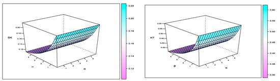
Figure 1. Three-dimensional plot of skewness and kurtosis with different values of parameters.

Table 1. Different measures of the moment by different values of parameters.

$\mathsf{\alpha }$	$\mathsf{\beta }$	Q1	Median	Q3	SK	KT
0.15	0.15	0.8973	2.2992	5.1031	0.33333	0.93528
	1.3	0.1035	0.2653	0.5888	0.33330	0.93527
	2.45	0.0549	0.1408	0.3124	0.33333	0.93536
	3.6	0.0374	0.0958	0.2126	0.33342	0.93537
	4.75	0.0283	0.0726	0.1611	0.33342	0.93564
1.5	0.15	2.2878	5.3284	10.2600	0.23720	0.63055
	1.3	0.2640	0.6148	1.1838	0.23721	0.63060
	2.45	0.1401	0.3262	0.6282	0.23723	0.63052
	3.6	0.0953	0.2220	0.4275	0.23719	0.63057
	4.75	0.0722	0.1683	0.3240	0.23715	0.63062
2.85	0.15	3.0063	6.5448	11.8495	0.19972	0.53889
	1.3	0.3469	0.7552	1.3673	0.19971	0.53887
	2.45	0.1841	0.4007	0.7255	0.19978	0.53887
	3.6	0.1253	0.2727	0.4937	0.19972	0.53893
	4.75	0.0949	0.2067	0.3742	0.19967	0.53882
4.2	0.15	3.5129	7.3072	12.7711	0.18033	0.49144
	1.3	0.4053	0.8431	1.4736	0.18035	0.49140
	2.45	0.2151	0.4474	0.7819	0.18030	0.49140
	3.6	0.1464	0.3045	0.5321	0.18043	0.49148
	4.75	0.1109	0.2308	0.4033	0.18031	0.49143

3. Estimation in the Classical Style

In this part, the classical point and interval estimation methods are discussed, namely maximum likelihood estimation for finding point estimates of R and asymptotic, boot-p, and boot-t intervals for R for obtaining interval estimates.

Maximum Likelihood R Estimation

Let $\mathrm{X}~\mathrm{APE}\left({\mathsf{\beta }}_1,\mathsf{\alpha }\right),\mathrm{Y}~\mathrm{APE}\left({\mathsf{\beta }}_2,\mathsf{\alpha }\right)$ and $\mathrm{Z}~\mathrm{APE}\left({\mathsf{\beta }}_3,\mathsf{\alpha }\right)$be independent functions.

Assuming $\mathsf{\alpha }$ is known in this the case, we have

$$\mathrm{R}=\mathrm{p}\left(\mathrm{X}<\mathrm{Y}<\mathrm{Z}\right)={{\displaystyle \int }}_{-\infty }^{\infty }{\mathrm{F}}_{\mathrm{X}}\left(\mathrm{y}\right){\mathrm{dF}}_{\mathrm{Y}}\left(\mathrm{y}\right)-{{\displaystyle \int }}_{-\infty }^{\infty }{\mathrm{F}}_{\mathrm{X}}\left(\mathrm{y}\right){\mathrm{F}}_{\mathrm{Z}}\left(\mathrm{y}\right){\mathrm{dF}}_{\mathrm{Y}}\left(\mathrm{y}\right),$$

(11)

$$=\frac{{\mathsf{\beta }}_1\left[2{\mathsf{\beta }}_1^2+2{\mathsf{\beta }}_2^2+0.5{\mathsf{\beta }}_3^2+1.5{\mathsf{\beta }}_1{\mathsf{\beta }}_3+3{\mathsf{\beta }}_1{\mathsf{\beta }}_2\right]}{\left({\mathsf{\beta }}_1+{\mathsf{\beta }}_2\right)\left({\mathsf{\beta }}_1+2{\mathsf{\beta }}_2\right)\left({\mathsf{\beta }}_1+{\mathsf{\beta }}_3\right)\left(2{\mathsf{\beta }}_1+{\mathsf{\beta }}_3\right)}$$

Figure 2 shows the different plot of multi-stress–strength reliability for different values of parameters, which explains that the multi-stress–strength reliability has different ranges.

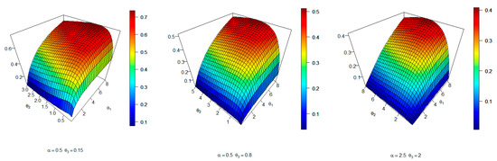
Figure 2. Three-dimensional plot of multi-stress–strength reliability with different values of parameters.

To obtain the MLE of R, we must first obtain the MLEs of ${\mathsf{\beta }}_1$, ${\mathsf{\beta }}_2$and ${\mathsf{\beta }}_3$. Let $\left({\mathrm{X}}_{1;{\mathrm{m}}_1,{\mathrm{n}}_1,{\mathrm{k}}_1},\dots ,{\mathrm{X}}_{{\mathrm{n}}_1;{\mathrm{m}}_1,{\mathrm{n}}_1,{\mathrm{k}}_1}\right),\left({\mathrm{Y}}_{1;{\mathrm{m}}_2,{\mathrm{n}}_2,{\mathrm{k}}_2},\dots ,{\mathrm{Y}}_{{\mathrm{n}}_2;{\mathrm{m}}_2,{\mathrm{n}}_2,{\mathrm{k}}_2}\right)$, and $\left({\mathrm{Z}}_{1;{\mathrm{m}}_3,{\mathrm{n}}_3,{\mathrm{k}}_3},\dots ,{\mathrm{Z}}_{{\mathrm{n}}_3;{\mathrm{m}}_3,{\mathrm{n}}_3,{\mathrm{k}}_3}\right)$ be three progressively first-failure censored samples from $\mathrm{APE}\left({\mathsf{\beta }}_{\mathrm{i}},\mathsf{\alpha }\right)$ distribution with censoring schemes ${\underset{¯}{\mathrm{R}}}_{\mathrm{x}}=\left({\mathrm{R}}_{{\mathrm{x}}_1},\dots ,{\mathrm{R}}_{{\mathrm{x}}_{\mathrm{m}1}}\right),{\underset{¯}{\mathrm{R}}}_{\mathrm{y}}=\left({\mathrm{R}}_{{\mathrm{y}}_1},\dots ,{\mathrm{R}}_{{\mathrm{y}}_{\mathrm{m}2}}\right),{\underset{¯}{\mathrm{R}}}_{\mathrm{z}}=\left({\mathrm{R}}_{{\mathrm{z}}_1},\dots ,{\mathrm{R}}_{{\mathrm{z}}_{\mathrm{m}3}}\right).$ Using the formulas from (2) and (3), the likelihood function of ${\mathsf{\beta }}_1$, ${\mathsf{\beta }}_2$and ${\mathsf{\beta }}_3$ is given by

$$\begin{array}{c}\mathrm{L}({\mathsf{\beta }}_1,{\mathsf{\beta }}_2,{\mathsf{\beta }}_3)\hfill \\ \propto {\displaystyle {\displaystyle \prod }_{\mathrm{j}=1}^3}{\left({\mathsf{\beta }}_{\mathrm{j}}{\mathrm{k}}_{\mathrm{j}}\right)}^{{\mathrm{m}}_{\mathrm{j}}}{\left(\frac{\log \mathsf{\alpha }}{\mathsf{\alpha }-1}\right)}^{\left({\mathrm{m}}_1+{\mathrm{m}}_2+{\mathrm{m}}_3\right)}{\displaystyle {\displaystyle \prod }_{\mathrm{i}=1}^{{\mathrm{m}}_1}}{\mathrm{e}}^{-{\mathsf{\beta }}_1{\mathrm{x}}_{\mathrm{i}}\left({\mathrm{k}}_1{\mathrm{R}}_{{\mathrm{x}}_{\mathrm{i}}}+1\right)}{\mathsf{\alpha }}^{1-{\mathrm{e}}^{-{\mathsf{\beta }}_1{\mathrm{x}}_{\mathrm{i}}\left({\mathrm{R}}_{{\mathrm{x}}_{\mathrm{i}}}+1\right)}}{\displaystyle {\displaystyle \prod }_{\mathrm{i}=1}^{{\mathrm{m}}_2}}{\mathrm{e}}^{-{\mathsf{\beta }}_2{\mathrm{y}}_{\mathrm{i}}\left({\mathrm{k}}_2{\mathrm{R}}_{{\mathrm{y}}_{\mathrm{i}}}+1\right)}{\mathsf{\alpha }}^{1-{\mathrm{e}}^{-{\mathsf{\beta }}_2{\mathrm{y}}_{\mathrm{i}}\left({\mathrm{k}}_2{\mathrm{R}}_{{\mathrm{y}}_{\mathrm{i}}}+1\right)}}\hfill \\ {\displaystyle {\displaystyle \prod }_{\mathrm{i}=1}^{{\mathrm{m}}_3}}{\mathrm{e}}^{-{\mathsf{\beta }}_3{\mathrm{z}}_{\mathrm{i}}\left({\mathrm{k}}_3{\mathrm{R}}_{{\mathrm{z}}_{\mathrm{i}}}+1\right)}{\mathsf{\alpha }}^{1-{\mathrm{e}}^{-{\mathsf{\beta }}_3{\mathrm{z}}_{\mathrm{i}}\left({\mathrm{k}}_3{\mathrm{R}}_{{\mathrm{z}}_{\mathrm{i}}}+1\right)}},\hfill \end{array}$$

(12)

We use ${\mathrm{x}}_{\mathrm{i}}$ instead of ${\mathrm{X}}_{{\mathrm{i}}_1;{\mathrm{m}}_1,{\mathrm{n}}_1,{\mathrm{k}}_1}$ to simplify notation. Similarity between ${\mathrm{y}}_{\mathrm{i}}$ and ${\mathrm{z}}_{\mathrm{i}}$.

The log-likelihood function, $\ell$ can now be written as follows:

$$\begin{array}{c}\mathsf{\ell }\left({\mathsf{\beta }}_1,{\mathsf{\beta }}_2,{\mathsf{\beta }}_3\right)\propto {{\displaystyle \sum }}_{j=1}^3{\mathrm{m}}_{\mathrm{j}}\left({\mathrm{lnk}}_{\mathrm{j}}+{\ln \mathsf{\beta }}_{\mathrm{j}}\right)+\left({\mathrm{m}}_1+{\mathrm{m}}_2+{\mathrm{m}}_3\right)\left[\ln \left(\log \mathsf{\alpha }\right)-\ln \left(\mathsf{\alpha }-1\right)\right]\hfill \\ -{{\displaystyle \sum }}_{i=1}^{{\mathrm{m}}_1}{\mathsf{\beta }}_1{\mathrm{x}}_{\mathrm{i}}\left({\mathrm{k}}_1{\mathrm{R}}_{{\mathrm{x}}_{\mathrm{i}}}+1\right)+{{\displaystyle \sum }}_{i=1}^{{\mathrm{m}}_1}\left(1-{\mathrm{e}}^{-{\mathsf{\beta }}_1{\mathrm{x}}_{\mathrm{i}}\left({\mathrm{R}}_{{\mathrm{x}}_{\mathrm{i}}}+1\right)}\right)\ln \left(\mathsf{\alpha }\right)-{{\displaystyle \sum }}_{i=1}^{{\mathrm{m}}_2}{\mathsf{\beta }}_2{\mathrm{y}}_{\mathrm{i}}\left({\mathrm{k}}_2{\mathrm{R}}_{{\mathrm{y}}_{\mathrm{i}}}+1\right)\hfill \\ +{{\displaystyle \sum }}_{i=1}^{{\mathrm{m}}_2}1-{\mathrm{e}}^{-{\mathsf{\beta }}_2{\mathrm{y}}_{\mathrm{i}}\left({\mathrm{k}}_2{\mathrm{R}}_{{\mathrm{y}}_{\mathrm{i}}}+1\right)}\ln \left(\mathsf{\alpha }\right)-{{\displaystyle \sum }}_{i=1}^{{\mathrm{m}}_3}{\mathsf{\beta }}_3{\mathrm{z}}_{\mathrm{i}}\left({\mathrm{k}}_3{\mathrm{R}}_{{\mathrm{z}}_{\mathrm{i}}}+1\right)+{{\displaystyle \sum }}_{i=1}^{{\mathrm{m}}_3}1-{\mathrm{e}}^{-{\mathsf{\beta }}_3{\mathrm{z}}_{\mathrm{i}}\left({\mathrm{k}}_3{\mathrm{R}}_{{\mathrm{z}}_{\mathrm{i}}}+1\right)}\ln \left(\mathsf{\alpha }\right)\hfill \end{array}$$

(13)

Taking the derivative of (14) with respect to β₁, β₂ and β₃, we obtain

$$\frac{\partial \ell }{\partial {\mathsf{\beta }}_1}=\frac{{\mathrm{m}}_1}{{\mathsf{\beta }}_1}-{{\displaystyle \sum }}_{i=1}^{{\mathrm{m}}_1}{\mathrm{x}}_{\mathrm{i}}\left({\mathrm{k}}_1{\mathrm{R}}_{{\mathrm{x}}_{\mathrm{i}}}+1\right)+\ln \left(\mathsf{\alpha }\right){{\displaystyle \sum }}_{i=1}^{{\mathrm{m}}_1}{\mathrm{x}}_{\mathrm{i}}\left({\mathrm{R}}_{{\mathrm{x}}_{\mathrm{i}}}+1\right){\mathrm{e}}^{-{\mathsf{\beta }}_1{\mathrm{x}}_{\mathrm{i}}\left({\mathrm{R}}_{{\mathrm{x}}_{\mathrm{i}}}+1\right)},$$

(14)

$$\frac{\partial \ell }{\partial {\mathsf{\beta }}_2}=\frac{{\mathrm{m}}_2}{{\mathsf{\beta }}_2}-{{\displaystyle \sum }}_{i=1}^{{\mathrm{m}}_2}{\mathrm{y}}_{\mathrm{i}}\left({\mathrm{k}}_2{\mathrm{R}}_{{\mathrm{y}}_{\mathrm{i}}}+1\right)+\ln \left(\mathsf{\alpha }\right){{\displaystyle \sum }}_{i=1}^{{\mathrm{m}}_2}{\mathrm{y}}_{\mathrm{i}}\left({\mathrm{k}}_2{\mathrm{R}}_{{\mathrm{y}}_{\mathrm{i}}}+1\right){\mathrm{e}}^{-{\mathsf{\beta }}_2{\mathrm{y}}_{\mathrm{i}}\left({\mathrm{k}}_2{\mathrm{R}}_{{\mathrm{y}}_{\mathrm{i}}}+1\right)}$$

(15)

$$\frac{\partial \ell }{\partial {\mathsf{\beta }}_3}=\frac{{\mathrm{m}}_3}{{\mathsf{\beta }}_3}-{{\displaystyle \sum }}_{i=1}^{{\mathrm{m}}_3}{\mathrm{z}}_{\mathrm{i}}\left({\mathrm{k}}_3{\mathrm{R}}_{{\mathrm{z}}_{\mathrm{i}}}+1\right)+\ln \left(\mathsf{\alpha }\right){{\displaystyle \sum }}_{i=1}^{{\mathrm{m}}_3}{\mathrm{z}}_{\mathrm{i}}\left({\mathrm{k}}_3{\mathrm{R}}_{{\mathrm{z}}_{\mathrm{i}}}+1\right){\mathrm{e}}^{-{\mathsf{\beta }}_3{\mathrm{z}}_{\mathrm{i}}\left({\mathrm{k}}_3{\mathrm{R}}_{{\mathrm{z}}_{\mathrm{i}}}+1\right)}$$

(16)

It is noted that the MLEs of ${\mathsf{\beta }}_1,{\mathsf{\beta }}_2$ and ${\mathsf{\beta }}_3$can not be found in closed form. Thus, by solving the system of nonlinear Equations (15)–(17), numerical solutions to the nonlinear system in (15)–(17) can be found using an iterative approach, such as Newton–Raphson. Then, the MLEs $\widehat{{\mathsf{\beta }}_1},$ $\widehat{{\mathsf{\beta }}_2}$ and $\widehat{{\mathsf{\beta }}_3}$ can be obtained. To obtain the MLE of R, by replacing ${\mathsf{\beta }}_1,{\mathsf{\beta }}_2$ and ${\mathsf{\beta }}_3$ in (5) with $\widehat{{\mathsf{\beta }}_1},$ $\widehat{{\mathsf{\beta }}_2}$ and $\widehat{{\mathsf{\beta }}_3}$ as follows:

$$\hat{\mathrm{R}}=\frac{{\hat{\mathsf{\beta }}}_1\left[2{\hat{\mathsf{\beta }}}_1^2+2{\hat{\mathsf{\beta }}}_2^2+0.5{\hat{\mathsf{\beta }}}_3^2+1.5{\hat{\mathsf{\beta }}}_1{\hat{\mathsf{\beta }}}_3+3{\hat{\mathsf{\beta }}}_1{\hat{\mathsf{\beta }}}_2\right]}{\left({\hat{\mathsf{\beta }}}_1+{\hat{\mathsf{\beta }}}_2\right)\left({\hat{\mathsf{\beta }}}_1+2{\hat{\mathsf{\beta }}}_2\right)\left({\hat{\mathsf{\beta }}}_1+{\hat{\mathsf{\beta }}}_3\right)\left(2{\hat{\mathsf{\beta }}}_1+{\hat{\mathsf{\beta }}}_3\right)}$$

(17)

4. Fisher Information

The Fisher information matrix of the $\mathsf{\phi }=\left({\mathsf{\beta }}_1,{\mathsf{\beta }}_2,{\mathsf{\beta }}_3\right)$ is expressed as

$$I_{3\times 3}=-E\left[\begin{array}{ccc}{A}_{11}& A_{12}& A_{13}\\ A_{21}& A_{22}& A_{23}\\ A_{31}& A_{32}& A_{33}\end{array}\right],$$

(18)

where $A_{11}=E\left(\frac{{\partial }^2\ell }{\partial {\mathsf{\beta }}_1^2}\right)$, $A_{12}=A_{21}=E\left(\frac{{\partial }^2\ell }{\partial {\mathsf{\beta }}_2\partial {\mathsf{\beta }}_1}\right)$, $A_{13}=A_{31}=E\left(\frac{{\partial }^2\ell }{\partial {\mathsf{\beta }}_1\partial {\mathsf{\beta }}_3}\right),$ $A_{22}=E\left(\frac{{\partial }^2\ell }{\partial {\mathsf{\beta }}_2^2}\right)$, $A_{23}=A_{32}=E\left(\frac{{\partial }^2\ell }{\partial {\mathsf{\beta }}_2\partial {\mathsf{\beta }}_3}\right)$ $A_{33}=E\left(\frac{{\partial }^2\ell }{\partial {\mathsf{\beta }}_3^2}\right)$,

$$\frac{{\partial }^2\ell }{\partial {\displaystyle {\mathsf{\beta }}_1^2}}=\frac{-{\mathrm{m}}_1}{{\mathsf{\beta }}_1^2}+\ln \left(\mathsf{\alpha }\right){{\displaystyle \sum }}_{i=1}^{{\mathrm{m}}_1}{\left[{\mathrm{x}}_{\mathrm{i}}\left({\mathrm{R}}_{{\mathrm{x}}_{\mathrm{i}}}+1\right)\right]}^2{\mathrm{e}}^{-{\mathsf{\beta }}_1{\mathrm{x}}_{\mathrm{i}}\left({\mathrm{R}}_{{\mathrm{x}}_{\mathrm{i}}}+1\right)},$$

$$\frac{{\partial }^2\ell }{\partial {\mathsf{\beta }}_2\partial {\mathsf{\beta }}_1}=\frac{{\partial }^2\ell }{\partial {\mathsf{\beta }}_1\partial {\mathsf{\beta }}_3}=\frac{{\partial }^2\ell }{\partial {\mathsf{\beta }}_2\partial {\mathsf{\beta }}_3}=0$$

$$\frac{{\partial }^2\ell }{\partial {\mathsf{\beta }}_2^2}=\frac{-{\mathrm{m}}_2}{{\mathsf{\beta }}_2}+\ln \left(\mathsf{\alpha }\right){{\displaystyle \sum }}_{i=1}^{{\mathrm{m}}_2}{\left[{\mathrm{y}}_{\mathrm{i}}\left({\mathrm{k}}_2{\mathrm{R}}_{{\mathrm{y}}_{\mathrm{i}}}+1\right)\right]}^2{\mathrm{e}}^{-{\mathsf{\beta }}_2{\mathrm{y}}_{\mathrm{i}}\left({\mathrm{k}}_2{\mathrm{R}}_{{\mathrm{y}}_{\mathrm{i}}}+1\right)},$$

$$\frac{{\partial }^2\ell }{\partial {\mathsf{\beta }}_3^2}=\frac{-{\mathrm{m}}_3}{{\mathsf{\beta }}_3}+\ln \left(\mathsf{\alpha }\right){\displaystyle {{\displaystyle \sum }}_{i=1}^{{\mathrm{m}}_3}}{\left[{\mathrm{z}}_{\mathrm{i}}\left({\mathrm{k}}_3{\mathrm{R}}_{{\mathrm{z}}_{\mathrm{i}}}+1\right)\right]}^2{\mathrm{e}}^{-{\mathsf{\beta }}_3{\mathrm{z}}_{\mathrm{i}}\left({\mathrm{k}}_3{\mathrm{R}}_{{\mathrm{z}}_{\mathrm{i}}}+1\right)}.$$

5. Confidence Intervals

In this section, the parameters’ confidence intervals (CIs) are computed. Because our point estimate is the most likely value for the parameter, we should build the confidence intervals on it. CIs are a set of values (intervals) that serve as good approximations of an unknown population parameter. In this investigation, two types of CIs were computed.

5.1. Approximate Confidence Intervals

Because the APE distribution’s PDF is not symmetric, asymptotic CIs based on normality do not perform well. The underlying distribution is assumed to be APE. As a result, we believe that the parametric bootstrap percentile interval is preferable to the nonparametric one. Furthermore, it is well known that the nonparametric bootstrap percentile interval does not perform well in general. See Section 5.3.1 of Ref. [45] for more information. The parametric bootstrap interval with normal approximation or Studentization can be used. However, because this CI is symmetric, it may not be suitable for our asymmetric instance. According to large sample theory, the MLE results are consistent and regularly distributed, subject to certain regularity restrictions. According to large sample theory, the MLE results are consistent and regularly distributed, subject to certain regularity restrictions. Because parameter MLE values are not in closed form, correct CIs cannot be obtained; instead, asymptotic CIs based on the asymptotic normal distribution of MLE values are computed.

Assume that $\mathsf{\phi }=\left({\mathsf{\beta }}_1,{\mathsf{\beta }}_2,{\mathsf{\beta }}_3,\mathrm{R}\right)$. $\left[\left(\widehat{{\mathsf{\beta }}_1}-{\mathsf{\beta }}_1\right),\left(\widehat{{\mathsf{\beta }}_2}-{\mathsf{\beta }}_2\right),\left(\widehat{{\mathsf{\beta }}_3}-{\mathsf{\beta }}_3\right),\left(\hat{\mathrm{R}}-\mathrm{R}\right)\right]$ is known to yield the asymptotic distribution of MLE values of $\mathrm{N}\left(0,\mathsf{\sigma }\right)$, where $\mathsf{\sigma }={\mathsf{\sigma }}_{\mathrm{ij}},\mathrm{i},\mathrm{j}=1,2,3,$ is the variance–covariance matrix of the unknown parameters. As previously established, the inverse of the Fisher information matrix is an estimator of the asymptomatic variance–covariance matrix.

The approximate $100\left(1-\mathsf{\omega }\right)\%$ two-sided CIs for $\mathsf{\phi }$ are provided by

$$\left({\hat{\mathsf{\phi }}}_{\mathrm{iL}},{\hat{\mathsf{\phi }}}_{\mathrm{iU}}\right):{\hat{\mathsf{\phi }}}_{\mathrm{i}}\mp {\mathrm{z}}_{1-\frac{\mathsf{\omega }}{2}}\sqrt{{\hat{\mathsf{\sigma }}}_{\mathrm{ij}}},\mathrm{i}=1,2,3,4.$$

(19)

where ${\mathrm{z}}_{1-\frac{\mathsf{\omega }}{2}}$ is the $100\left(1-\frac{\mathsf{\omega }}{2}\right)$-th upper percentile of the standard normal distribution.

5.2. Bootstrap Confidence Intervals

In this paragraph, we propose to employ two additional confidence intervals based on parametric bootstrap methods: percentile bootstrap technique (Boot-p) and bootstrap-t method (Boot-t). Obtaining the step-by-step illustrations of the two ways is shown briefly below; for more information, see Ref. [46].

5.2.1. Methods of Boot-p

• Use the sample $\left\{{\mathrm{X}}_{1;{\mathrm{m}}_1,{\mathrm{n}}_1,{\mathrm{k}}_1},\dots ,{\mathrm{X}}_{{\mathrm{m}}_1;{\mathrm{m}}_1,{\mathrm{n}}_1,{\mathrm{k}}_1}\right\},\left\{{\mathrm{Y}}_{1;{\mathrm{m}}_2,{\mathrm{n}}_2,{\mathrm{k}}_2},\dots ,{\mathrm{Y}}_{{\mathrm{m}}_2;{\mathrm{m}}_2,{\mathrm{n}}_2,{\mathrm{k}}_2}\right\},\mathrm{and}\left\{{\mathrm{Z}}_{1;{\mathrm{m}}_3,{\mathrm{n}}_3,{\mathrm{k}}_3},\dots ,{\mathrm{Z}}_{{\mathrm{m}}_3;{\mathrm{m}}_3,{\mathrm{n}}_3,{\mathrm{k}}_3}\right\}$ to compute $\widehat{{\mathsf{\beta }}_1},\widehat{{\mathsf{\beta }}_2}$and $\widehat{{\mathsf{\beta }}_3}$.
• Based on ${\underset{¯}{\mathrm{R}}}_{\mathrm{x}}$ censoring technique, a bootstrap progressive first-failure Type-II censored sample indicated by ${\mathrm{X}}_{1;{\mathrm{m}}_1,{\mathrm{n}}_1,{\mathrm{k}}_1}^{*},\dots ,{\mathrm{X}}_{{\mathrm{m}}_1;{\mathrm{m}}_1,{\mathrm{n}}_1,{\mathrm{k}}_1}^{*}$ is constructed from the $\mathrm{APE}\left(\mathsf{\alpha },{\mathsf{\beta }}_1\right).$ From the $\mathrm{APE}\left(\mathsf{\alpha },{\mathsf{\beta }}_2\right)$, a bootstrap progressive first-failure Type-II censored sample designated by ${\mathrm{Y}}_{1;{\mathrm{m}}_2,{\mathrm{n}}_2,{\mathrm{k}}_2}^{*},\dots ,{\mathrm{Y}}_{{\mathrm{m}}_2;{\mathrm{m}}_2,{\mathrm{n}}_2,{\mathrm{k}}_2}^{*}$ is constructed using ${\underset{¯}{\mathrm{R}}}_{\mathrm{y}}$ censoring scheme. Based on ${\underset{¯}{\mathrm{R}}}_{\mathrm{z}}$ censoring scheme, a bootstrap progressive first-failure Type-II censored sample, indicated by ${\mathrm{Z}}_{1;{\mathrm{m}}_3,{\mathrm{n}}_3,{\mathrm{k}}_3}^{*},\dots ,{\mathrm{Z}}_{{\mathrm{m}}_3;{\mathrm{m}}_3,{\mathrm{n}}_3,{\mathrm{k}}_3}^{*}$, is constructed from the $\mathrm{APE}\left(\mathsf{\alpha },{\mathsf{\beta }}_3\right).$Based on $\left\{{\mathrm{X}}_{1;{\mathrm{m}}_1,{\mathrm{n}}_1,{\mathrm{k}}_1}^{*},\dots ,{\mathrm{X}}_{{\mathrm{m}}_1;{\mathrm{m}}_1,{\mathrm{n}}_1,{\mathrm{k}}_1}^{*}\right\},\left\{{\mathrm{Y}}_{1;{\mathrm{m}}_2,{\mathrm{n}}_2,{\mathrm{k}}_2}^{*},\dots ,{\mathrm{Y}}_{{\mathrm{m}}_2;{\mathrm{m}}_2,{\mathrm{n}}_2,{\mathrm{k}}_2}^{*}\right\},$and $\left\{{\mathrm{Z}}_{1;{\mathrm{m}}_3,{\mathrm{n}}_3,{\mathrm{k}}_3}^{*},\dots ,{\mathrm{Z}}_{{\mathrm{m}}_3;{\mathrm{m}}_3,{\mathrm{n}}_3,{\mathrm{k}}_3}^{*}\right\}$, construct the bootstrap sample estimate of R using (5), say ${\hat{\mathrm{R}}}^{*}$.
• Step 2 should be repeated ${\mathrm{N}}_{\mathrm{p}}$ times.
• Assume $\mathrm{G}\left(\mathrm{x}\right)=\mathrm{P}\left({\hat{\mathrm{R}}}^{*}\le \mathrm{x}\right)$, where ${\hat{\mathrm{R}}}^{*}$ is the cumulative distribution function. For a given $\mathrm{x}$, define ${\hat{\mathrm{R}}}_{\mathrm{Boot}-\mathrm{p}}\left(\mathrm{x}\right)={\mathrm{G}}^{-1}\left(\mathrm{x}\right).$ The approximation of $100\left(1-\mathsf{\omega }\right)\%$ percent confidence interval of $\mathrm{R}$ is given by

  $$\left({\hat{\mathrm{R}}}_{\mathrm{Boot}-\mathrm{p}}\left(\frac{\mathsf{\omega }}{2}\right),{\hat{\mathrm{R}}}_{\mathrm{Boot}-\mathrm{p}}\left(1-\frac{\mathsf{\omega }}{2}\right)\right).$$

5.2.2. Methods of Boot-t

• Use the sample$\left\{{\mathrm{X}}_{1;{\mathrm{m}}_1,{\mathrm{n}}_1,{\mathrm{k}}_1},\dots ,{\mathrm{X}}_{{\mathrm{m}}_1;{\mathrm{m}}_1,{\mathrm{n}}_1,{\mathrm{k}}_1}\right\},$ $\left\{{\mathrm{Y}}_{1;{\mathrm{m}}_2,{\mathrm{n}}_2,{\mathrm{k}}_2},\dots ,{\mathrm{Y}}_{{\mathrm{m}}_2;{\mathrm{m}}_2,{\mathrm{n}}_2,{\mathrm{k}}_2}\right\},$ and $\left\{{\mathrm{Z}}_{1;{\mathrm{m}}_3,{\mathrm{n}}_3,{\mathrm{k}}_3},\dots ,{\mathrm{Z}}_{{\mathrm{m}}_3;{\mathrm{m}}_3,{\mathrm{n}}_3,{\mathrm{k}}_3}\right\}$ to compute $\widehat{{\mathsf{\beta }}_1},\widehat{{\mathsf{\beta }}_2}$and $\widehat{{\mathsf{\beta }}_3}$.
• Use ${\hat{\mathsf{\beta }}}_1$ to generate a bootstrap sample ${\mathrm{X}}_{1;{\mathrm{m}}_1,{\mathrm{n}}_1,{\mathrm{k}}_1}^{*},\dots ,{\mathrm{X}}_{{\mathrm{m}}_1;{\mathrm{m}}_1,{\mathrm{n}}_1,{\mathrm{k}}_1}^{*}$, ${\hat{\mathsf{\beta }}}_2$ to generate a bootstrap sample ${\mathrm{Y}}_{1;{\mathrm{m}}_2,{\mathrm{n}}_2,{\mathrm{k}}_2}^{*},\dots ,{\mathrm{Y}}_{{\mathrm{m}}_2;{\mathrm{m}}_2,{\mathrm{n}}_2,{\mathrm{k}}_2}^{*}$, and similarly, ${\hat{\mathsf{\beta }}}_3$ to generate a bootstrap sample ${\mathrm{Z}}_{1;{\mathrm{m}}_3,{\mathrm{n}}_3,{\mathrm{k}}_3}^{*},\dots ,{\mathrm{Z}}_{{\mathrm{m}}_3;{\mathrm{m}}_3,{\mathrm{n}}_3,{\mathrm{k}}_3}^{*}$. Based on $\left\{{\mathrm{X}}_{1;{\mathrm{m}}_1,{\mathrm{n}}_1,{\mathrm{k}}_1}^{*},\dots ,{\mathrm{X}}_{{\mathrm{m}}_1;{\mathrm{m}}_1,{\mathrm{n}}_1,{\mathrm{k}}_1}^{*}\right\}$, $\left\{{\mathrm{Y}}_{1;{\mathrm{m}}_2,{\mathrm{n}}_2,{\mathrm{k}}_2}^{*},\dots ,{\mathrm{Y}}_{{\mathrm{m}}_2;{\mathrm{m}}_2,{\mathrm{n}}_2,{\mathrm{k}}_2}^{*}\right\}$ and $\left\{{\mathrm{Z}}_{1;{\mathrm{m}}_3,{\mathrm{n}}_3,{\mathrm{k}}_3}^{*},\dots ,{\mathrm{Z}}_{{\mathrm{m}}_3;{\mathrm{m}}_3,{\mathrm{n}}_3,{\mathrm{k}}_3}^{*}\right\}$, compute the bootstrap sample estimate of R using (5), say ${\hat{\mathrm{R}}}^{*}$ and the following statistic:

  $${\mathrm{T}}^{*}=\frac{\sqrt{\mathrm{m}}\left({\hat{\mathrm{R}}}^{*}-\hat{\mathrm{R}}\right)}{\sqrt{\mathrm{V}\left({\hat{\mathrm{R}}}^{*}\right)}}$$
• Step 2 should be repeated ${\mathrm{N}}_{\mathrm{p}}$ times.
• After obtaining ${\mathrm{N}}_{\mathrm{p}}$ a number of ${\mathrm{T}}^{*}$ values, the boundaries $100\left(1-\mathsf{\omega }\right)\%$ of $\mathrm{R}$ percent confidence interval are determined as follows: Assume ${\mathrm{T}}^{*}$ has a cumulative distribution function given by $\mathrm{H}\left(\mathrm{x}\right)=\mathrm{P}\left({\mathrm{T}}^{*}\le \mathrm{x}\right).$ Define ${\hat{\mathrm{R}}}_{\mathrm{Boot}-\mathrm{t}}=\hat{\mathrm{R}}+\sqrt{\mathrm{V}\left(\hat{\mathrm{R}}\right)\mathrm{m}}{\mathrm{H}}^{-1}\left(\mathrm{x}\right)$ for a given $\mathrm{x}$.
• $100\left(1-\mathsf{\omega }\right)\%$ percent boot-t confidence interval of $\mathrm{R}$is calculated as $\left({\hat{\mathrm{R}}}_{\mathrm{Boot}-\mathrm{t}}\left(\frac{\mathsf{\omega }}{2}\right),{\hat{\mathrm{R}}}_{\mathrm{Boot}-\mathrm{t}}\left(1-\frac{\mathsf{\omega }}{2}\right)\right)$
• To achieve better estimates of parameters or any function of parameters, it is often advantageous to incorporate prior knowledge about the parameters, which could be prior data, expert opinion, or some other medium of knowledge. A Bayesian technique is used to include such prior knowledge into the estimation process. As a result, we now go through the Bayesian approach of estimation in depth, which incorporates previous knowledge in the form of prior distributions.

6. Bayesian Approach

Bayesian inference has gained appeal in a variety of sectors in recent years, including engineering, clinical medicine, biology, and so on. Its capacity to analyze data using prior knowledge makes it valuable in dependability studies, where data availability is a major issue. The model parameters ${\mathsf{\beta }}_1,{\mathsf{\beta }}_2,{\mathsf{\beta }}_3$ and $\mathrm{R}$ Bayesian estimates, as well as the corresponding credible intervals, are derived in this section.

6.1. Prior Information and Loss Function

Because the gamma distribution can take on different shapes based on the parameter values, using various gamma priors is simple and can result in more expressive posterior density estimates. As a result, we investigated gamma density priors, which are more adaptable than other challenging prior distributions and APE distribution under progressive first-failure censoring model parameters. As a result, under progressive first-failure censoring model parameters gamma $\left({\mathrm{a}}_{\mathrm{j}},{\mathrm{b}}_{\mathrm{j}}\right);\mathrm{j}=1,\dots ,4$, independent gamma PDFs are assumed for the APE distribution. The joint prior is as follows

$$\mathsf{\pi }\left({\mathsf{\beta }}_1,{\mathsf{\beta }}_2,{\mathsf{\beta }}_3,\mathrm{R}\right)\propto {\mathsf{\beta }}_1{}^{{\mathrm{a}}_1-1}{\mathrm{e}}^{-{\mathrm{b}}_1{\mathsf{\beta }}_1}{\mathsf{\beta }}_2^{{\mathrm{a}}_2-1}{\mathrm{e}}^{-{\mathrm{b}}_2{\mathsf{\beta }}_2}{\mathsf{\beta }}_3^{{\mathrm{a}}_3-1}{\mathrm{e}}^{-{\mathrm{b}}_3{\mathsf{\beta }}_3}{\mathrm{R}}^{{\mathrm{a}}_4-1}{\mathrm{e}}^{-{\mathrm{b}}_4\mathrm{R}},$$

(20)

where ${\mathrm{a}}_{\mathrm{j}},{\mathrm{b}}_{\mathrm{j}};\mathrm{j}=1,\dots ,4$ indicate prior knowledge of the unknown parameters ${\mathsf{\beta }}_1,{\mathsf{\beta }}_2,{\mathsf{\beta }}_3$ and R and are anticipated to be non-negative.

According to the literature, choosing the symmetric loss function (SLF), (squared loss function) (SEL) is a critical issue in Bayesian analysis. The SEL function is the most often utilized SLF in this study for estimating the considered unknown values.

$$ℒ\left(\mathrm{R},\tilde{\mathrm{R}}\right)={\left(\tilde{\mathrm{R}}-\mathrm{R}\right)}^2, ℒ\left({\mathsf{\beta }}_1,\widetilde{{\mathsf{\beta }}_1}\right)={\left(\widetilde{{\mathsf{\beta }}_1}-{\mathsf{\beta }}_1\right)}^2, ℒ\left({\mathsf{\beta }}_2,\widetilde{{\mathsf{\beta }}_2}\right)={\left(\widetilde{{\mathsf{\beta }}_2}-{\mathsf{\beta }}_2\right)}^2, ℒ\left({\mathsf{\beta }}_3,\widetilde{{\mathsf{\beta }}_3}\right)={\left(\widetilde{{\mathsf{\beta }}_3}-{\mathsf{\beta }}_3\right)}^2,$$

where $\tilde{\mathrm{R}},\widetilde{{\mathsf{\beta }}_1},\widetilde{{\mathsf{\beta }}_2}$ and $\widetilde{{\mathsf{\beta }}_3}$are approximations of $\mathrm{R},{\mathsf{\beta }}_1,{\mathsf{\beta }}_2$ and ${\mathsf{\beta }}_3$. The posterior mean of $\mathrm{R},{\mathsf{\theta }}_1,{\mathsf{\theta }}_2$ and ${\mathsf{\theta }}_3$is utilized to compute the objective estimate of$\tilde{\mathrm{R}},\widetilde{{\mathsf{\theta }}_1},\widetilde{{\mathsf{\theta }}_2},$ and $\widetilde{{\mathsf{\theta }}_3}$. In contrast, any other loss function can be easily incorporated.

6.2. Posterior Analysis by SLF

Observing the APE distribution under progressive first-failure censoring sample data from the likelihood function and the prior knowledge given both yield the joint posterior density function.

$$\mathrm{L}\left(\mathrm{R},{\mathsf{\beta }}_1,{\mathsf{\beta }}_2,{\mathsf{\beta }}_3|\underset{\_}{\mathrm{t}}\right)\propto \mathsf{\pi }\left(\mathrm{R},{\mathsf{\beta }}_1,{\mathsf{\beta }}_2,{\mathsf{\beta }}_3\right){{\displaystyle \prod }}_{\mathrm{i}=1}^3{{\displaystyle \prod }}_{\mathrm{j}=1}^{{\mathrm{n}}_{\mathrm{i}}}\mathrm{g}\left({\mathrm{t}}_{\mathrm{ij}}\right){\left(1-\mathrm{G}\left({\mathrm{t}}_{\mathrm{ij}}\right)\right)}^{{\mathrm{c}}_{\mathrm{i}}},$$

(21)

The Bayesian estimator of $\mathrm{R},{\mathsf{\theta }}_1,{\mathsf{\theta }}_2$ and ${\mathsf{\theta }}_3$ such as $\tilde{\mathrm{R}},\widetilde{{\mathsf{\theta }}_1},\widetilde{{\mathsf{\theta }}_2},$ and $\widetilde{{\mathsf{\theta }}_3}$, under the SEL function, is the posterior expectation of $\mathrm{R},{\mathsf{\theta }}_1,{\mathsf{\theta }}_2$ and ${\mathsf{\theta }}_3$. The marginal posterior distributions for each of the parameters ($\mathrm{R},{\mathsf{\theta }}_1,{\mathsf{\theta }}_2$ and ${\mathsf{\theta }}_3$) must be gathered in order to generate these estimates. However, due to the implied mathematical calculations, precise formulations for the marginal PDFs for each unknown parameter are plainly not realistic. As a result, we would like to generate Bayesian estimates and credible intervals utilizing simulation approaches such as MCMC.

The Metropolis–Hastings (MH) algorithm, which is used to generate random samples using the posterior density distribution and an independent proposal distribution to approximate Bayesian estimates and to create the associated Highest Posterior Density (HPD) credible intervals, is one of the most useful MCMC algorithms. In addition, this method provides a chain version of the Bayesian estimate that is simple to use in practice.

7. Optimization Criterion

In recent years, there has been a lot of interest in finding the optimal censoring scheme in the statistical literature; for example, see Refs. [47,48,49,50,51,52,53]. Possible censoring schemes refer to any ${\mathrm{R}}_1,\dots ,{\mathrm{R}}_{\mathrm{m}}$ combinations such that $\mathrm{n}=\mathrm{m}+{{\displaystyle \sum }}_{\mathrm{i}=1}^{\mathrm{m}}{\mathrm{R}}_{\mathrm{i}}$ and finding the optimum sampling approach means locating the progressive censoring scheme that offers the most information about the unknown parameters among all conceivable progressive censoring schemes for fixed $\mathrm{n}$ and $\mathrm{m}$. The first difficulty is, of course, how to generate unknown parameter information measures based on specific progressive censoring data, and the second is how to compare two distinct information measures based on two different progressive censoring techniques. The next subsections go through some of the optimality criteria that were employed in this situation. In practice, we want to select the filtering scheme that delivers the most information about the unknown parameters; see Ref. [54] for further information. In our example, Table 2 presents a number of regularly used measures to help us choose the appropriate progressive censoring approach.

Table 2. Some practical censoring plan optimum criteria.

Criterion	Method
${\mathrm{O}}_1$	Maximize trace $\left[I_{3\times 3}(.)\right]$
${\mathrm{O}}_2$	Minimize trace ${\left[I_{3\times 3}(.)\right]}^{-1}$
${\mathrm{O}}_3$	Minimize det ${\left[I_{3\times 3}(.)\right]}^{-1}$
${\mathrm{O}}_4$	Minimize $Var\left[log\left({\hat{\mathrm{t}}}_{\mathrm{p}}\right)\right], 0<p<1$

In terms of ${\mathrm{O}}_1$, our goal is to maximize the observed Fisher $I_{3\times 3}(.)$ information values. Furthermore, our goal for criterion ${\mathrm{O}}_2$ and ${\mathrm{O}}_3$ is to minimize the determinant and trace of ${\left[I_{3\times 3}(.)\right]}^{-1}$. Comparing multiple criteria is simple when dealing with single-parameter distributions; however, when dealing with unknown multi-parameter distributions, comparing the two Fisher information matrices becomes more difficult because the criterion ${\mathrm{O}}_2$ and ${\mathrm{O}}_3$ are not scale-invariant; see Ref. [55]. However, the optimal censoring scheme of multi-parameter distributions can be chosen using scale-invariant criteria ${\mathrm{O}}_4$. The criterion ${\mathrm{O}}_4$, which is dependent on the value of $\mathrm{p}$, clearly tends to minimize the variance of logarithmic MLE of the $\mathrm{p}-\mathrm{th}$ quantile, $\log \left({\hat{\mathrm{t}}}_{\mathrm{p}}\right)$. As a result, the logarithmic for ${\hat{\mathrm{t}}}_{\mathrm{p}}$ of the APE distribution is supplied by

$$\log \left({\hat{\mathrm{t}}}_{\mathrm{p}}\right)=\log \left\{\frac{-1}{\mathsf{\beta }}\log \left[1-\frac{\log \left(\mathrm{p}\left(\mathsf{\alpha }-1\right)\right)}{\log \mathsf{\alpha }}\right]\right\},0<\mathrm{p}<1,$$

The delta approach is applied to (3) to produce the approximated variance for $\log \left({\hat{\mathrm{t}}}_{\mathrm{p}}\right)$of the APE distribution as

$$\mathrm{Var}\left(\log \left({\hat{\mathrm{t}}}_{\mathrm{p}}\right)\right)={\left[\nabla \log \left({\hat{\mathrm{t}}}_{\mathrm{p}}\right)\right]}^{\mathrm{T}}{\mathrm{I}}_{3\times 3}^{-1}\left({\hat{\mathsf{\beta }}}_1,{\hat{\mathsf{\beta }}}_2,{\hat{\mathsf{\beta }}}_3\right)\left[\nabla \log \left({\hat{\mathrm{t}}}_{\mathrm{p}}\right)\right],$$

where

$${\left[\nabla \log \left({\hat{\mathrm{t}}}_{\mathrm{p}}\right)\right]}^{\mathrm{T}}={\left[\frac{\partial }{\partial {\mathsf{\beta }}_1}\log \left({\hat{\mathrm{t}}}_{\mathrm{p}}\right),\frac{\partial }{\partial {\mathsf{\beta }}_2}\log \left({\hat{\mathrm{t}}}_{\mathrm{p}}\right),\frac{\partial }{\partial {\mathsf{\beta }}_3}\log \left({\hat{\mathrm{t}}}_{\mathrm{p}}\right)\right]}_{\left({\mathsf{\beta }}_1=\widehat{{\mathsf{\beta }}_1},{\mathsf{\beta }}_2=\widehat{{\mathsf{\beta }}_2},{\mathsf{\beta }}_3=\widehat{{\mathsf{\beta }}_3}\right)}.$$

The optimal progressive censoring, however, corresponds to a maximum value of the criterion ${\mathrm{O}}_1$ and a minimum value of the criteria ${\mathrm{O}}_{\mathrm{i}}$ $\mathrm{i},=1,2,3,4.$

8. Simulation Study

A simulation study is carried out to illustrate the relative efficiency of multi-stress–strength reliability under the progressive first failure based on different censored schemes and to evaluate it as a function of changing factors of a parameter. For a better understanding of this model, we use the following procedure to produce samples from the progressive first failure based on different censored schemes for APE distribution described in Section 3.

A large number N = 1000 of progressively first-failure censored samples for a true value of parameters $\mathsf{\alpha },{\mathsf{\beta }}_1,{\mathsf{\beta }}_2,$ and ${\mathsf{\beta }}_3$ different combinations of n (number of groups), m (progressively first-failure-censoring data), and k (number of items within each group) are generated from the APE by using the algorithm described in Balakrishnan and Sandhu (1995). In each case, the MLE and Bayesian of the multi-stress–strength reliability are computed. The asymptotic CIs and two parametric bootstrap CIs are used for MLE computation purposes. The HPD CIs are used for Bayesian computation purposes. The MSE and Bias values are used to compare different estimators. The average lengths are also used to compare the performances of the two-sided 95% asymptotic CI/HPD credible intervals, where the length of asymptotic CI is (LACI), length of bootstrap-p CI is (LBPCI), length of bootstrap-t CI is (LBTCI), and length of credible CI is (LCCI). Comparison between censoring schemes is made with respect to their optimum criteria measures; see Table 1, where we consider the various sampling schemes listed as follows:

• Scheme I: ${\mathrm{R}}_{\mathrm{m}}=\mathrm{n}-\mathrm{m}$ and ${\mathrm{R}}_{\mathrm{i}}=0;\mathrm{i}=1,\dots ,\mathrm{m}-1$,
• Scheme II: ${\mathrm{R}}_1=\mathrm{n}-\mathrm{m}$ and ${\mathrm{R}}_{\mathrm{i}}=0;\mathrm{i}=2,\dots ,\mathrm{m}$.

The simulation study was conducted with various values of (k, n, m), such as n = 20, 50, and k = 2 and 4 for each group size. When the number of failed participants reaches or exceeds a specified value m, the test is over, where m =12 and 18 when n = 20, and m = 35 and 45 when n = 50. The joint posterior distribution of the unknown four parameters is proportional to the likelihood function based on the non-informative priors of hyper-parameters ai, bi for I = 1, …, 4. As a result, we employed an informative prior of, and using elective hyper-parameters, the values of hyper-parameters are chosen to satisfy the prior mean, resulting in the expected value of the corresponding parameter; see Refs. [56,57]. The Bayesian estimation based on 12,000 MCMC samples and discarding the first 2000 values as “burn-in” are generated using the M-H sampler technique introduced in Section 3.

The progressive first failure of censored samples was generated from APE distribution for four sets of parametric values:

• In Table 2: $\mathsf{\alpha }=0.8,{\mathsf{\beta }}_1=1.8,{\mathsf{\beta }}_2=0.8,{\mathsf{\beta }}_3=0.2$ and $\mathsf{\alpha }=2,{\mathsf{\beta }}_1=1.8,{\mathsf{\beta }}_2=0.8,{\mathsf{\beta }}_3=0.2$.
• In Table 3: $\mathsf{\alpha }=0.8,{\mathsf{\beta }}_1=3,{\mathsf{\beta }}_2=2,{\mathsf{\beta }}_3=1.5$ and $\mathsf{\alpha }=2,{\mathsf{\beta }}_1=3,{\mathsf{\beta }}_2=2,{\mathsf{\beta }}_3=1.5$.
  Table 3. MLE and Bayesian point and interval estimations for multi-stress–strength reliability with optimality measures when ${\mathsf{\beta }}_1 = 1.8,{\mathsf{\beta }}_2 = 0.8,{\mathsf{\beta }}_3 = 0.2$.

  ${\mathsf{\beta }}_1=1.8,{\mathsf{\beta }}_2=0.8,{\mathsf{\beta }}_3=0.2$					MLE		Bayesian		MLE			HPD	Optimality
  $\mathsf{\alpha }$	n	k	Scheme	m	Bias	MSE	Bias	MSE	LACI	LBPCI	LBTCI	LCCI	O1	O2	O3
  0.8	20	2	I	12	0.0244	0.0051	0.0491	0.0038	0.2621	0.0085	0.0083	0.1397	21.3816	0.00079670	1315.0742
  				18	0.0137	0.0031	0.0487	0.0029	0.2099	0.0065	0.0064	0.0909	4.1313	0.00000699	1860.8153
  			II	12	0.0142	0.0051	0.0257	0.0019	0.2750	0.0083	0.0086	0.1332	6.5200	0.00010403	1137.2594
  				18	0.0152	0.0027	0.0402	0.0021	0.1966	0.0063	0.0062	0.0807	3.2014	0.00000570	1541.9155
  		4	I	12	0.0231	0.0043	0.0215	0.0041	0.2271	0.0072	0.0071	0.1299	32.0128	0.00002417	4326.9511
  				18	0.0110	0.0023	0.0103	0.0021	0.1695	0.0054	0.0053	0.0757	7.1082	0.00000042	5887.7508
  			II	12	0.0218	0.0038	0.0179	0.0037	0.2274	0.0071	0.0072	0.1124	13.6802	0.00001076	4260.3735
  				18	0.0278	0.0024	0.0020	0.0020	0.1602	0.0052	0.0052	0.0689	5.7489	0.00000036	4892.7823
  	50	2	I	35	−0.0026	0.0019	0.0025	0.0015	0.1694	0.0076	0.0076	0.1309	5.4335	0.00000781	2173.0070
  				45	−0.0018	0.0013	0.0016	0.0013	0.1399	0.0062	0.0062	0.0876	0.9871	0.00000027	2673.3238
  			II	35	0.0038	0.0027	−0.0034	0.0008	0.2033	0.0093	0.0095	0.1027	1.4849	0.00000062	1446.0044
  				45	0.0026	0.0020	0.0233	0.0010	0.1764	0.0079	0.0080	0.0801	1.0515	0.00000015	1889.7725
  		4	I	35	0.0016	0.0029	−0.0039	0.0005	0.2119	0.0099	0.0099	0.0795	2.7322	0.00000005	4818.0247
  				45	0.0054	0.0018	0.0341	0.0016	0.1642	0.0070	0.0071	0.0688	1.8893	0.000000008	6547.6266
  			II	35	0.0148	0.0016	0.0408	0.0015	0.1434	0.0062	0.0062	0.0693	1.9652	0.00000001	12,058.2247
  				45	0.0171	0.0010	0.0740	0.0010	0.1042	0.0047	0.0047	0.0534	1.4447	0.000000002	14,466.0555
  2	20	2	I	12	0.0252	0.0053	0.0389	0.0029	0.2687	0.0122	0.0118	0.1378	44.8698	0.00028752	1298.6571
  				18	0.0138	0.0025	0.0383	0.0019	0.1901	0.0083	0.0083	0.0824	10.6874	0.000007058	1724.2822
  			II	12	0.0118	0.0047	0.0151	0.0012	0.2650	0.0118	0.0119	0.1133	18.6539	0.00006624	1221.1348
  				18	0.0138	0.0028	0.0319	0.0014	0.1998	0.0090	0.0090	0.0797	10.2767	0.000007664	1692.4905
  		4	I	12	0.0362	0.0044	0.0958	0.0041	0.2189	0.0098	0.0097	0.1120	71.0129	0.00003361	3458.2427
  				18	0.0305	0.0023	0.0739	0.0022	0.1469	0.0064	0.0065	0.0646	17.4184	0.000000603	4725.7657
  			II	12	0.0284	0.0053	0.0352	0.0018	0.2632	0.0123	0.0124	0.0918	30.5605	0.000007690	3241.6188
  				18	0.0311	0.0027	0.0570	0.0025	0.1628	0.0072	0.0073	0.0606	14.7362	0.00000051	4491.3445
  	50	2	I	35	0.0149	0.0018	0.0475	0.0018	0.1565	0.0069	0.0071	0.0939	6.3239	0.000000503	3853.6782
  				45	0.0119	0.0012	0.0396	0.0011	0.1287	0.0058	0.0056	0.0564	2.9557	0.00000007	4607.4580
  			II	35	0.0120	0.0016	0.0029	0.0004	0.1479	0.0066	0.0067	0.0780	3.5200	0.000000218	3587.6918
  				45	0.0135	0.0011	0.0278	0.0010	0.1215	0.0053	0.0054	0.0543	2.6907	0.00000007	4509.7376
  		4	I	35	0.0305	0.0020	0.0796	0.0017	0.1285	0.0059	0.0058	0.0817	13.5622	0.000000060	9487.8097
  				45	0.0247	0.0013	0.0652	0.0012	0.1001	0.0046	0.0047	0.0521	5.5558	0.00000001	12,885.4276
  			II	35	0.0264	0.0019	0.0119	0.0003	0.1350	0.0060	0.0060	0.0459	5.9567	0.000000015	10,036.4394
  				45	0.0253	0.0014	0.0402	0.0013	0.1085	0.0048	0.0048	0.0480	4.1892	0.00000000	12,893.1857

In computational analysis, extensive computations were carried out using the R statistical programming language software, with the “coda” package proposed by Ref. [58], and the “maxLik” package proposed by Henningsen and Toomet (2011), which uses the Newton–Raphson method of maximizing the computations. The average results of MLE and Bayesian for multi-stress–strength reliability are presented in Table 2 and Table 3.

Table 3 and Table 4 show that APE based on the multi-stress–strength model MLE and Bayesian of multi-stress–strength reliability is excellent in terms of MSE, Bias, and CI length (LCI). The MSE, Bias, and LCI drop as n and m rise, as expected. Furthermore, the MSE, Bias, and LCI drop as group size k grows. In terms of MSE, Bias, and LCI, Bayesian estimation utilizing gamma informative prior is also superior to MLE because it includes prior knowledge. In terms of the length of CI values, HPD credible intervals outperform asymptotic CI for interval estimation. As a result, we recommend using the M-H approach to estimate multi-stress–strength reliability using Bayesian point and interval estimates. Furthermore, when comparing Scheme I and Scheme II, it is obvious that the MLE optimum criteria measures for Scheme II are higher than for Scheme I.

Table 4. MLE and Bayesian point and interval estimations for multi-stress–strength reliability with optimality measures when ${\mathsf{\beta }}_1 = 3,{\mathsf{\beta }}_2 = 2,{\mathsf{\beta }}_3 = 1.5$.

${\mathsf{\beta }}_1=3,{\mathsf{\beta }}_2=2,{\mathsf{\beta }}_3=1.5$					MLE		Bayesian		MLE			HPD	Optimality
$\mathsf{\alpha }$	n	k	Scheme	m	Bias	MSE	Bias	MSE	LACI	LBPCI	LBTCI	LCCI	O1	O2	O3
0.8	20	2	I	12	0.0141	0.0035	0.0204	0.0015	0.2243	0.0098	0.0095	0.1263	32.7192	0.851629	59.1656
				18	0.0062	0.0020	0.0075	0.0004	0.1737	0.0079	0.0078	0.0721	5.3389	0.007162	95.2781
			II	12	0.0054	0.0041	0.0079	0.0010	0.2489	0.0109	0.0109	0.1141	8.4620	0.140559	93.5644
				18	0.0041	0.0020	0.0066	0.0004	0.1755	0.0076	0.0077	0.0753	3.8724	0.005310	68.8098
		4	I	12	0.0086	0.0017	0.0514	0.0014	0.1601	0.0069	0.0071	0.1405	41.6896	0.040229	181.3487
				18	0.0101	0.0011	0.0207	0.0008	0.1233	0.0056	0.0057	0.0726	8.0888	0.000366	197.4359
			II	12	0.0060	0.0029	0.0252	0.0017	0.2111	0.0093	0.0093	0.1170	10.7009	0.005277	123.4315
				18	0.0108	0.0014	0.0160	0.0006	0.1426	0.0062	0.0061	0.0715	5.8162	0.000307	140.7154
	50	2	I	35	0.0053	0.0011	0.0412	0.0010	0.1291	0.0056	0.0055	0.1019	5.5126	0.000537	262.9994
				45	0.0019	0.0006	0.0163	0.0006	0.0982	0.0043	0.0042	0.0641	1.7133	0.000035	247.1240
			II	35	0.0038	0.0010	0.0161	0.0008	0.1262	0.0056	0.0057	0.0920	1.4508	0.000110	130.4385
				45	0.0002	0.0007	0.0114	0.0004	0.1059	0.0048	0.0047	0.0648	1.0404	0.000031	148.3842
		4	I	35	0.0028	0.0005	0.0923	0.0004	0.0857	0.0038	0.0039	0.1058	7.7591	0.000029	704.7141
				45	0.0025	0.0003	0.0411	0.0002	0.0723	0.0033	0.0033	0.0717	2.8182	0.000002	710.6756
			II	35	0.0046	0.0009	0.0333	0.0006	0.1163	0.0052	0.0053	0.0854	2.1859	0.000007	399.3411
				45	0.0055	0.0005	0.0279	0.0004	0.0836	0.0037	0.0039	0.0686	1.6343	0.000002	465.4802
2	20	2	I	12	0.0111	0.0030	0.0250	0.0019	0.2118	0.0095	0.0094	0.1366	48.2769	0.309823	47.0611
				18	0.0096	0.0021	0.0070	0.0004	0.1750	0.0078	0.0080	0.0737	12.2381	0.008539	65.7453
			II	12	0.0031	0.0036	0.0084	0.0011	0.2352	0.0106	0.0105	0.1259	19.2689	0.059121	39.0353
				18	0.0088	0.0020	0.0062	0.0004	0.1710	0.0073	0.0074	0.0710	10.0978	0.006465	53.7042
		4	I	12	0.0121	0.0018	0.0592	0.0015	0.1611	0.0071	0.0071	0.1328	73.0888	0.029018	112.0391
				18	0.0117	0.0011	0.0215	0.0009	0.1243	0.0056	0.0056	0.0815	17.7696	0.000577	137.7838
			II	12	0.0064	0.0027	0.0247	0.0015	0.2010	0.0090	0.0091	0.1186	16.6365	0.001927	101.0923
				18	0.0106	0.0013	0.0151	0.0006	0.1342	0.0060	0.0062	0.0770	11.7618	0.000317	136.2249
	50	2	I	35	0.0033	0.0009	0.0416	0.0008	0.1198	0.0055	0.0055	0.0975	6.9337	0.000501	111.1543
				45	0.0022	0.0007	0.0165	0.0006	0.1023	0.0045	0.0045	0.0632	3.0112	0.000064	143.9309
			II	35	0.0034	0.0011	0.0105	0.0006	0.1271	0.0059	0.0058	0.0869	3.6038	0.000188	110.5934
				45	0.0040	0.0008	0.0100	0.0004	0.1094	0.0049	0.0049	0.0686	2.6286	0.000058	140.2241
		4	I	35	0.0113	0.0006	0.0822	0.0005	0.0895	0.0039	0.0037	0.0869	13.8108	0.000054	281.3838
				45	0.0089	0.0005	0.0375	0.0004	0.0780	0.0036	0.0036	0.0656	5.6687	0.000006	388.0669
			II	35	0.0100	0.0010	0.0195	0.0007	0.1191	0.0054	0.0056	0.0689	5.7857	0.000014	313.3802
				45	0.0093	0.0004	0.0238	0.0004	0.0839	0.0037	0.0036	0.0595	4.3141	0.000004	395.1895

9. Application of Real Data

The analysis of real data is presented in this part for demonstration reasons. We look at data from three distinct voltages of 36, 34, and 32 KV that show times to breakdown of an insulating fluid between electrodes. This information is taken from page 105 of [59].

Data set 1: Times to breakdown of an insulated fluid at 32 KV (Z): 0.27, 0.40, 0.69, 0.79, 0.75, 2.75, 3.91, 9.88, 13.95, 15.93, 27.80, 53.24, 82.85, 89.29, 100.58, 215.10.

Data set 2: Times to breakdown of an insulated fluid at 34 KV (Y): 0.19, 0.78, 0.96, 1.31, 2.78, 3.16, 4.15, 4.67, 4.85, 6.50,7.35, 8.01, 8.27, 12.06, 31.75, 32.52, 33.91, 36.71, 72.89.

Data set 3: Times to breakdown of an insulated fluid at 36 KV (X): 0.35, 0.59, 0.96, 0.99, 1.69, 1.97, 2.07, 2.58, 2.71, 2.90,3.67, 3.99, 5.35, 13.77, 25.50.

Ref. [60] discusses the estimation of R = P[Y < X < Z] of the Weibull distribution. Table 5 discusses parameter estimation with stander error (SE) for this model and R = P[Y < X < Z] by the MLE method.

Table 5. MLE with SE and R = P[Y < X < Z] for the Weibull model.

	Estimates	SE	Lower	Upper
$\mathsf{\beta }$	0.6813	0.0911	0.5026	0.8599
${\mathsf{\theta }}_1$	0.6861	0.2586	0.1793	1.1928
${\mathsf{\theta }}_2$	0.4150	0.1424	0.1358	0.6942
${\mathsf{\theta }}_3$	0.2266	0.0892	0.0518	0.4015
R	0.3342

First, we check the fitting of APE distribution to this data; see Table 6. Distance of Kolmogorov–Smirnov (DKS) with p values (PVKS) for three distinct voltages data. The values of KSD statistics are found to be 0.2598, 0.1612, and 0.1427 with corresponding PVKS 0.2214, 0.6492, and 0.8786. The p values indicate that the APE distribution with the above-mentioned parameters is a suitable model for modeling these three data sets. The plots of the estimated PDF, CDF, and PP plot of the three data sets in Figure 3, Figure 4 and Figure 5 also confirm the same.

Table 6. MLE with SE, KSD, and different measures for three distinct voltages data.

		Estimates	SE	KSD	PVKS	VAIC	VBIC	VCVM	VAD
x1	$\mathsf{\alpha }$	0.0854	0.1495	0.2598	0.2214	142.1859	143.6020	0.0431	0.3264
	$\mathsf{\beta }$	0.0147	0.0082
x2	$\mathsf{\alpha }$	0.1094	0.2142	0.1612	0.6492	140.8927	142.7816	0.0584	0.3580
	$\mathsf{\beta }$	0.0409	0.0253
x3	$\mathsf{\alpha }$	0.0421	0.1392	0.1427	0.8786	77.8128	79.2289	0.0669	0.4317
	$\mathsf{\beta }$	0.0943	0.0885

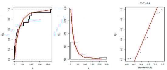
Figure 3. Plots of the estimated PDF, CDF, and PP of APE distribution in data set I.

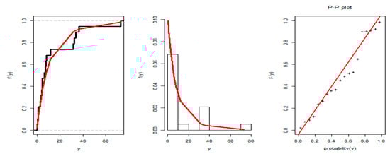
Figure 4. Plots of the estimated PDF, CDF and PP plot of APE distribution in data set II.

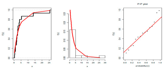
Figure 5. Plots of the estimated PDF, CDF, and PP plot of APE distribution in data set III.

Based on the complete data, the MLE and Bayesian estimate for the APE model of R = P[Y < X < Z] are found to be 0.4523 and 0.4570, respectively, as shown in Table 7. Here, it is to be noted in the Bayesian estimation of parameters that we use informative priors, as gamma prior is available regarding the model parameters. From the results of Table 7, we show that the Bayesian estimation is the best estimation of this model where the multi-stress–strength reliability R = P[Y < X < Z] is larger than MLE. In addition, the SE of Bayesian is smaller than MLE. Figure 6 shows the contour plot of the log-likelihood function of this model with different values of parameters to check the unique and global values of these parameters. Figure 7 discusses the MCMC trace, convergence, and plot of the posterior distribution of this model.

Table 7. MLE and Bayesian estimation for the parameters and R = P[Y < X < Z] for the APE model.

	MLE				Bayesian
	Estimates	SE	Lower	Upper	Estimates	SE	Lower	Upper
$\mathsf{\alpha }$	0.0811	0.0168	0.0481	0.2791	0.0837	0.0125	0.0426	0.1297
${\mathsf{\beta }}_1$	0.1126	0.0515	0.0116	0.2135	0.1252	0.0444	0.0485	0.2212
${\mathsf{\beta }}_2$	0.0375	0.0173	0.0036	0.0714	0.0405	0.0102	0.0167	0.0663
${\mathsf{\beta }}_3$	0.0145	0.0066	0.0014	0.0275	0.0156	0.0035	0.0053	0.0275
R	0.4523				0.4570

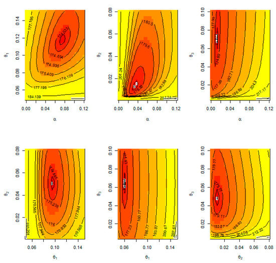
Figure 6. Contour plot of log-likelihood function with different values of parameters; complete sample.

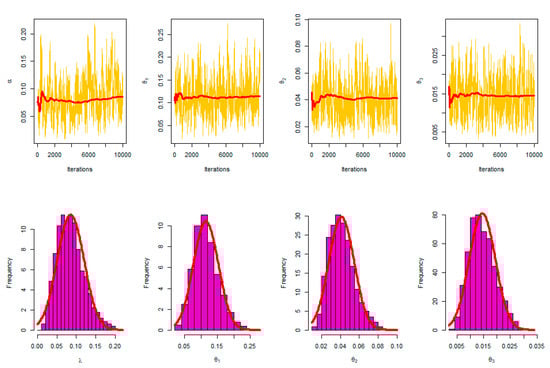
Figure 7. MCMC trace, convergence and plot of posterior distribution; complete sample.

10. Conclusions

In this paper, inference for multi-reliability using unit alpha power exponential distributions for stress–strength variables based on the progressive first failure is considered. The conventional methods such as maximum likelihood and Bayesian methods for point estimation of the parameter model and R are obtained. The Fisher information and confidence intervals such as asymptotic, boot-p, and boot-t methods are also examined. Various optimal criteria have been found. Monte Carlo simulations and real-world application examples are used to evaluate and compare the performance of the various proposed estimators.

References

- Weerahandi, S.; Johnson, R.A. Testing reliability in a stress-strength model when X and Y are normally distributed. Technometrics 1992, 34, 83–91. [Google Scholar] [CrossRef]
- Surles, J.G.; Padgett, W.J. Inference for reliability and stress-strength for a scaled Burr Type X distribution. Lifetime Data Anal. 2001, 7, 187–200. [Google Scholar] [CrossRef] [PubMed]
- Al-Mutairi, D.K.; Ghitany, M.E.; Kundu, D. Inferences on stress-strength reliability from Lindley distributions. Commun. Stat.—Theory Methods 2013, 42, 1443–1463. [Google Scholar] [CrossRef]
- Rao, G.S.; Aslam, M.; Kundu, D. Burr-XII distribution parametric estimation and estimation of reliability of multicomponent stress-strength. Commun. Stat.—Theory Methods 2015, 44, 4953–4961. [Google Scholar] [CrossRef]
- Singh, S.K.; Singh, U.; Yaday, A.; Viswkarma, P.K. On the estimation of stress strength reliability parameter of inverted exponential distribution. Int. J. Sci. World 2015, 3, 98–112. [Google Scholar] [CrossRef][Green Version]
- Abo-Kasem, O.E.; Almetwally, E.M.; Abu El Azm, W.S. Inferential Survival Analysis for Inverted NH Distribution Under Adaptive Progressive Hybrid Censoring with Application of Transformer Insulation. Ann. Data Sci. 2022, 1–48. [Google Scholar] [CrossRef]
- Alshenawy, R.; Sabry, M.A.; Almetwally, E.M.; Almongy, H.M. Product Spacing of Stress-Strength under Progressive Hybrid Censored for Exponentiated-Gumbel Distribution. Comput. Mater. Contin. 2021, 66, 2973–2995. [Google Scholar] [CrossRef]
- Alamri, O.A.; Abd El-Raouf, M.M.; Ismail, E.A.; Almaspoor, Z.; Alsaedi, B.S.; Khosa, S.K.; Yusuf, M. Estimate stress-strength reliability model using Rayleigh and half-normal distribution. Comput. Intell. Neurosci. 2021, 7653581. [Google Scholar] [CrossRef]
- Sabry, M.A.; Almetwally, E.M.; Alamri, O.A.; Yusuf, M.; Almongy, H.M.; Eldeeb, A.S. Inference of fuzzy reliability model for inverse Rayleigh distribution. AIMS Math. 2021, 6, 9770–9785. [Google Scholar] [CrossRef]
- Abu El Azm, W.S.; Almetwally, E.M.; Alghamdi, A.S.; Aljohani, H.M.; Muse, A.H.; Abo-Kasem, O.E. Stress-Strength Reliability for Exponentiated Inverted Weibull Distribution with Application on Breaking of Jute Fiber and Carbon Fibers. Comput. Intell. Neurosci. 2021, 4227346. [Google Scholar] [CrossRef]
- Okabe, T.; Otsuka, Y. Proposal of a Validation Method of Failure Mode Analyses based on the Stress-Strength Model with a Support Vector Machine. Reliab. Eng. Syst. Saf. 2021, 205, 107247. [Google Scholar] [CrossRef]
- Bhattacharyya, G.K.; Johnson, R.A. Estimation of reliability in a multicomponent stress-strength model. J. Am. Stat. Assoc. 1974, 69, 966–970. [Google Scholar] [CrossRef]
- Kotb, M.S.; Raqab, M.Z. Estimation of reliability for multi-component stress–strength model based on modified Weibull distribution. Stat. Pap. 2021, 62, 2763–2797. [Google Scholar] [CrossRef]
- Maurya, R.K.; Tripathi, Y.M. Reliability estimation in a multicomponent stress-strength model for Burr XII distribution under progressive censoring. Braz. J. Probab. Stat. 2020, 34, 345–369. [Google Scholar] [CrossRef]
- Mahto, A.K.; Tripathi, Y.M.; Kızılaslan, F. Estimation of Reliability in a Multicomponent Stress-Strength Model for a General Class of Inverted Exponentiated Distributions Under Progressive Censoring. J. Stat. Theory Pract. 2020, 14, 58. [Google Scholar] [CrossRef]
- Alotaibi, R.M.; Tripathi, Y.M.; Dey, S.; Rezk, H.R. Bayesian and non-Bayesian reliability estimation of multicomponent stress–strength model for unit Weibull distribution. J. Taibah Univ. Sci. 2020, 14, 1164–1181. [Google Scholar] [CrossRef]
- Maurya, R.K.; Tripathi, Y.M.; Kayal, T. Reliability Estimation in a Multicomponent Stress-Strength Model Based on Inverse Weibull Distribution. Sankhya B 2022, 84, 364–401. [Google Scholar] [CrossRef]
- Chandra, S.; Owen, D.B. On estimating the reliability of a component subject to several different stresses (strengths). Nav. Res. Logist. Quart. 1975, 22, 31–39. [Google Scholar]
- Dutta, K.; Sriwastav, G.L. An n-standby system with P(X < Y < Z). IAPQR Trans. 1986, 12, 95–97. [Google Scholar]
- Ivshin, V.V. On the estimation of the probabilities of a double linear inequality in the case of uniform and two-parameter exponential distributions. J. Math. Sci. 1998, 88, 819–827. [Google Scholar] [CrossRef]
- Singh, N. On the estimation of Pr(X1 < Y < X2). Commun. Statist. Theory Meth. 1980, 9, 1551–1561. [Google Scholar]
- Hlawka, P. Estimation of the Parameter p = P(X < Y < Z); No.11, Ser. Stud. i Materiaty No. 10 Problemy Rachunku Prawdopodobienstwa; Prace Nauk. Inst. Mat. Politechn.: Wroclaw, Poland, 1975; pp. 55–65. [Google Scholar]
- Hanagal, D.D. Estimation of system reliability in multicomponent series stress-strength model. J. Indian Statist. Assoc. 2003, 41, 1–7. [Google Scholar]
- Waegeman, W.; De Baets, B.; Boullart, L. On the scalability of ordered multi-class ROC analysis. Comput. Statist. Data Anal. 2008, 52, 33–71. [Google Scholar] [CrossRef]
- Chumchum, D.; Munindra, B.; Jonali, G. Cascade System with Pr(X < Y < Z). J. Inform. Math. Sci. 2013, 5, 37–47. [Google Scholar]
- Patowary, A.N.; Sriwastav, G.L.; Hazarika, J. Inference of R = P(X < Y < Z) for n-Standby System: A Monte-Carlo Simulation Approach. J. Math. 2016, 12, 18–22. [Google Scholar]
- Yousef, M.M.; Almetwally, E.M. Multi stress-strength reliability based on progressive first failure for Kumaraswamy model: Bayesian and non-Bayesian estimation. Symmetry 2021, 13, 2120. [Google Scholar] [CrossRef]
- Kohansal, A.; Shoaee, S. Bayesian and classical estimation of reliability in a multicomponent stress-strength model under adaptive hybrid progressive censored data. Stat. Pap. 2021, 62, 309–359. [Google Scholar] [CrossRef]
- Saini, S.; Tomer, S.; Garg, R. On the reliability estimation of multicomponent stress–strength model for Burr XII distribution using progressively first-failure censored samples. J. Stat. Comput. Simul. 2022, 92, 667–704. [Google Scholar] [CrossRef]
- Kohansal, A.; Fernández, A.J.; Pérez-González, C.J. Multi-component stress–strength parameter estimation of a non-identical component strengths system under the adaptive hybrid progressive censoring samples. Statistics 2021, 55, 925–962. [Google Scholar] [CrossRef]
- Hassan, M.K. On Estimating Standby Redundancy System in a MSS Model with GLFRD Based on Progressive Type II Censoring Data. Reliab. Theory Appl. 2021, 16, 206–219. [Google Scholar]
- Alotaibi, R.; Tripathi, Y.; Dey, S.; Rezk, H. Estimation of multicomponent reliability based on progressively Type II censored data from unit Weibull distribution. WSEAS Trans. Math. 2021, 20, 288–299. [Google Scholar] [CrossRef]
- Wu, S.J.; Kus, C. On estimation based on progressive first-failure-censored sampling. Comput. Stat. Data Anal. 2009, 53, 3659–3670. [Google Scholar] [CrossRef]
- Balakrishnan, N.; Aggarwala, R. Progressive Censoring: Theory, Methods, and Applications; Springer Science & Business Media Birkhauser Boston: Cambridge, MA, USA, 2000. [Google Scholar]
- Mahdavi, A.; Kundu, D. A new method for generating distributions with an application to exponential distribution. Commun. Stat. Theory Methods 2017, 46, 6543–6557. [Google Scholar] [CrossRef]
- Nassar, M.; Alzaatreh, A.; Mead, M.; Abo-Kasem, O. Alpha power Weibull distribution: Properties and applications. Commun. Stat.—Theory Methods 2017, 46, 10236–10252. [Google Scholar] [CrossRef]
- Dey, A.; Alzaatreh, A.; Zhang, C.; Kumar, D. A new extension of generalized exponential distribution with application to ozone data. Ozone Sci. Eng. 2017, 39, 273–285. [Google Scholar] [CrossRef]
- Nadarajah, S.; Okorie, I.E. On the moments of the alpha power transformed generalized exponential distribution. Ozone Sci. Eng. 2018, 40, 330–335. [Google Scholar] [CrossRef]
- Alotaibi, R.; Elshahhat, A.; Rezk, H.; Nassar, M. Inferences for Alpha Power Exponential Distribution Using Adaptive Progressively Type-II Hybrid Censored Data with Applications. Symmetry 2022, 14, 651. [Google Scholar] [CrossRef]
- Alotaibi, R.; Al Mutairi, A.; Almetwally, E.M.; Park, C.; Rezk, H. Optimal Design for a Bivariate Step-Stress Accelerated Life Test with Alpha Power Exponential Distribution Based on Type-I Progressive Censored Samples. Symmetry 2022, 14, 830. [Google Scholar] [CrossRef]
- Dence, T.P.; Dence, J.B. A survey of Euler’s constant. Math. Mag. 2009, 82, 255–265. [Google Scholar] [CrossRef]
- Abramowitz, M.; Stegun, I.A. Handbook of Mathematical Functions: With Formulas, Graphs, and Mathematical Tables; 55 of National Bureau of Standards Applied Mathematics Series; U.S. Government Printing Office: Washington, DC, USA, 1964.
- Seaborn, J.B. Hypergeometric Functions and Their Applications; Springer: New York, NY, USA, 1991. [Google Scholar]
- Wolfram Research, Inc. Mathematica—Wolfram/Alpha; Davison and Hinkley: Champaign, IL, USA, 1997. [Google Scholar]
- Davison, A.C.; Hinkley, D.V. Bootstrap Methods and Their Application; Cambridge University Press: Cambridge, UK, 1997. [Google Scholar]
- Tibshirani, R.; Efron, B. An Introduction to the Bootstrap; Chapman & Hall, Inc.: New York, NY, USA, 1993. [Google Scholar]
- Ng, H.K.T.; Chan, C.S.; Balakrishnan, N. Optimal progressive censoring plans for the Weibull distribution. Technometrics 2004, 46, 470–481. [Google Scholar] [CrossRef]
- Balasooriya, U.; Balakrishnan, N. Reliability sampling plans for log-normal distribution, based on progressively-censored samples. IEEE Trans. Reliab. 2000, 49, 199–203. [Google Scholar] [CrossRef]
- Balasooriya, U.; Saw, S.L.C.; Gadag, V. Progressively censored reliability sampling plans for the Weibull distribution. Technometrics 2000, 42, 160–167. [Google Scholar] [CrossRef]
- Burkschat, M.; Cramer, E.; Kamps, U. Optimality criteria and optimal schemes in progressive censoring. Commun. Stat.—Theory Methods 2007, 36, 1419–1431. [Google Scholar] [CrossRef]
- Burkschat, M.; Cramer, E.; Kamps, U. On optimal schemes in progressive censoring. Stat. Probab. Lett. 2006, 76, 1032–1036. [Google Scholar] [CrossRef]
- Burkschat, M. On optimality of extremal schemes in progressive type II censoring. J. Stat. Plan. Inference 2008, 138, 1647–1659. [Google Scholar] [CrossRef]
- Pradhan, B.; Kundu, D. On progressively censored generalized exponential distribution. Test 2009, 18, 497–515. [Google Scholar] [CrossRef]
- Elshahhat, A.; Rastogi, M.K. Estimation of parameters of life for an inverted Nadarajah–Haghighi distribution from Type-II progressively censored samples. J. Indian Soc. Probab. Stat. 2021, 22, 113–154. [Google Scholar] [CrossRef]
- Gupta, R.D.; Kundu, D. On the comparison of Fisher information of the Weibull and GE distributions. J. Stat. Plan. Inference 2006, 136, 3130–3144. [Google Scholar] [CrossRef]
- Almongy, H.M.; Alshenawy, F.Y.; Almetwally, E.M.; Abdo, D.A. Applying transformer insulation using Weibull extended distribution based on progressive censoring scheme. Axioms 2021, 10, 100. [Google Scholar] [CrossRef]
- El-Sherpieny, E.S.A.; Almetwally, E.M.; Muhammed, H.Z. Bayesian and non-bayesian estimation for the parameter of bivariate generalized Rayleigh distribution based on clayton copula under progressive type-II censoring with random removal. Sankhya A 2021, 1–38. [Google Scholar] [CrossRef]
- Plummer, M.; Best, N.; Cowles, K.; Vines, K. CODA: Convergence diagnosis and output analysis for MCMC. R News 2006, 6, 7–11. [Google Scholar]
- Nelson, W.B. Applied Life Data Analysis; John Wiley & Sons.: Hoboken, NJ, USA, 2003. [Google Scholar]
- Choudhary, N.; Tyagi, A.; Singh, B. Estimation of R = P[Y < X < Z] under Progressive Type-II Censored Data from Weibull Distribution. Lobachevskii J. Math. 2021, 42, 318–335. [Google Scholar]
Publisher’s Note: MDPI stays neutral with regard to jurisdictional claims in published maps and institutional affiliations. |
© 2022 by the authors. Licensee MDPI, Basel, Switzerland. This article is an open access article distributed under the terms and conditions of the Creative Commons Attribution (CC BY) license (https://creativecommons.org/licenses/by/4.0/).