An Autonomous Storage Optimization LRM Generation Strategy Based on Cascaded NURBS

Abstract

Automatic control of intelligent vehicles depends heavily on accurate lane-level location information. The traditional digital map cannot meet the automatic driving requirements, and it is very difficult for lane-level road maps (LRMs) to achieve a good balance between the representation accuracy and data storage volume. To tackle this problem, we obtain the recursive definition of a lane line by analyzing road lanes using the fractal geometry theory. Subsequently, we construct a recursive feedback system and model it. On this basis, an autonomous storage optimization LRM generation strategy based on cascaded NURBS is devised. According to the input data density, this framework generates an LRM with the minimum data storage volume within the error constraint. It is mainly composed of two modules: (1) a random fractal and (2) an adaptive iteration memory optimizer, based on cascaded NURBS error feedback. First, the whole lane is divided into several meta lane line modules. Second, data sampling/interpolation is carried out iteratively according to the NURBS fitting error and symmetry of road geometry. In this way, the storage space used to store lane lines and other information is automatically optimized. Last, a simulation experiment is carried out by using a dataset obtained from a park. The simulation results show that the proposed method can achieve high accuracy and high storage efficiency. Under the constraint of a 0.1 m curve fitting error, the average memory demand of the lane line elements is less than 2.4 bytes/m.

1. Introduction

A lane-level road map (LRM) is a kind of map that shows micro-scale details, including lane lines, lane markers, and other elements. It facilitates high-precision lane-level positioning for vehicles and plays an important role in the accomplishment of various tasks such as lane-level path planning and high-precision self-positioning of intelligent vehicles [1]. Intelligent vehicles can completely accomplish environmental perception and decision-making tasks without any human intervention. The accuracies of environmental perception and environmental elements models such as lane lines directly affect the driving safety, trafficability, and riding experience. An accurate LRM is required in order to enable advanced driver assistance systems (ADAS) to effectively perform their functions, such as lane keeping, lane change assistance, etc. [2]. The precision of automatic control of intelligent vehicles depends heavily on positioning information and LRM accuracy. LRMs can provide much necessary information for autonomous driving, such as lane line information, reference path information, etc. However, their storage capacity can reduce the efficiency of data interaction and increase the computational load. It is necessary to reduce the consumption of physical storage by lane-level maps as much as possible while ensuring the application accuracy.

The data required for building an LRM can be obtained by combining road markings such as lane lines, road arrows, etc. These markings are obtained through mature environmental perception algorithms using the information provided by the high-precision positioning module [3]. Usually, a straight line and an arc are used to model and represent the obtained lane lines and other elements for storage and use, but the continuity at the junction points is not guaranteed. A lane line that has significant curvature needs to be divided into multiple segments in order to attain a specific accuracy level. For a large lane curvature, the lane may need to be divided into shorter segments in order to achieve a specific level of position accuracy. Alternatively, it is feasible to divide a lane line into multiple segments and model each segment using polynomials. However, this can cause the Runge effect and curve oscillations.

From a technical point of view, the maps of automatic driving vehicle systems must have sufficient levels of accuracy, storage efficiency, and availability [2]. LRMs need to accurately represent the shapes of all lane lines, including straight lines, arcs, inclinations, etc. In addition, the geometry of each lane line should be conducive to reducing the data storage space and calculation workload, and should be easily modifiable in order to improve the access speed and availability of the map.

In order to meet the requirements of real-world applications, researchers have carried out extensive research in this field. A few researchers have proposed a host of curve models to accurately represent the lane line elements in the map, such as multiple segment polygons [4,5], circular arc splines [6,7], cubic B-spline [8,9], clothoid splines [10], B-spline, and so on.

Polygons have been widely used to create various digital road maps. A road is often divided into multiple segments in order to meet the accuracy requirement, which increases the data storage volume. A smooth arc spline is a curve consisting of smoothly connected arcs and line segments. The offset curve of a circular arc spline is also an arc spline, usually not a polygon, polynomial spline, or line segment, and the calculation of the offset curve is related to the generation of continuous map elements, allowing for accurate offset and arc length calculations. It is convenient to calculate the distance from the point to the curve. Unlike that of clothoid curves, the curvature of circular arc curves [6,7] is a step function and cannot output a smooth amount of steering wheel control.

The cubic spline curve [8] (cubic Elmitian spline curve) is a representative interpolated spline curve. The advantage of natural cubic splines is the ease of representing the road model using only path points. Road geometry can be effectively represented by cubic spline curves with low computational load.

In order to ensure smoothness, some researchers use clothoids to connect a straight line and an arc in order to represent a lane line [11]. However, one drawback of defining clothoids [12,13] using the Fresnel integral is the huge workload of mapping calculation and operation; therefore, this method was not pursued further in this study [4]. The curve constructed using segment polynomials can be used to approximate real lane lines. This method allows for a convenient local modification, but is not suitable for processing large-scale lane line data because the time complexity of calculation often reaches O (n³) [2].

A spline curve has good properties. In order to ensure the approximation accuracy and storage efficiency of lane lines, many researchers choose B-spline [14] as the mathematical model of a road. It retains the advantages of Bezier and at the same time overcomes one of its major deficiencies, i.e., the lack of local properties due to overall representation. In addition, B-spline supports piecewise smoothing and smoothing of connection between segments. It has a few excellent properties that most spline functions do not have, such as recursion, local support, continuous order adjustment, etc. Furthermore, it can be calculated conveniently and allows for engineering modification and access. Moreover, it allows for uniform modeling of polynomial splines of different orders and continuity levels. However, a lane line often contains a large number of quadratic arc curves, whereas the B-spline and other methods can only give an approximate representation of the quadratic arcs, which will cause extra errors and affect the final accuracy. Based on the B-spline, NURBS introduces the weight factor and denominator, which not only retains the B-spline’s strong ability to represent free shapes, but also expands its ability to uniformly and accurately represent conic arcs. Due to this reason, we selected NURBS [15] as the curve model. Apart from storing control points, NURBS needs to store the corresponding weight factors, which increases the data storage volume.

In this study, we took certain measures to tackle the aforementioned problems. The key contributions of this study are as follows:

• Lane lines are analyzed by using the fractal geometry theory to obtain the recursive definition of a lane line. A recursive feedback system is constructed based on the idea of dynamic programming, and its convergence is proved theoretically, which provides a theoretical basis for developing the autonomous storage optimization LRM generation strategy based on the cascaded NURBS.
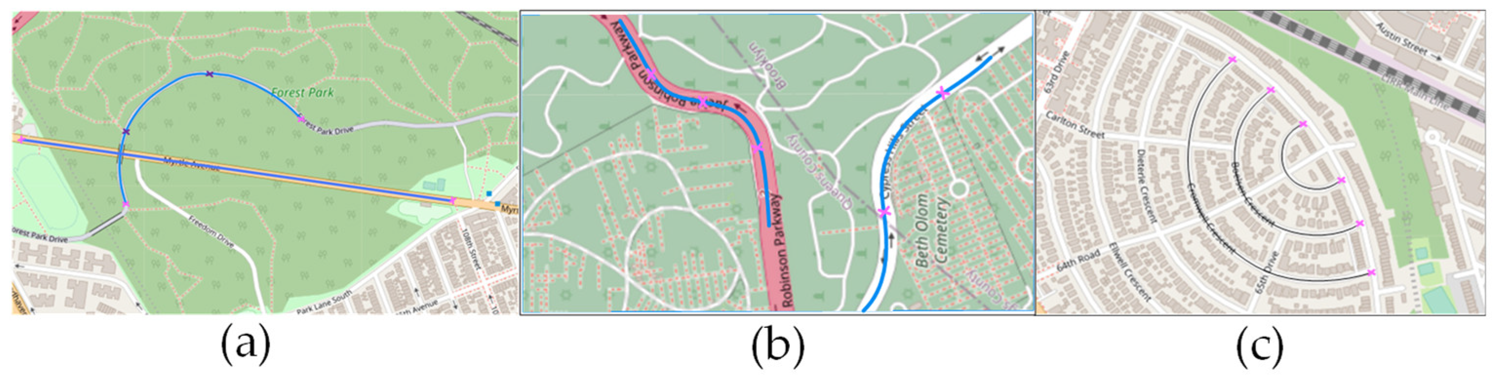
• A random shape-dividing algorithm is designed for lane lines to recognize and segment the obtained lane lines and divide the lane line data set into a meta lane line set.
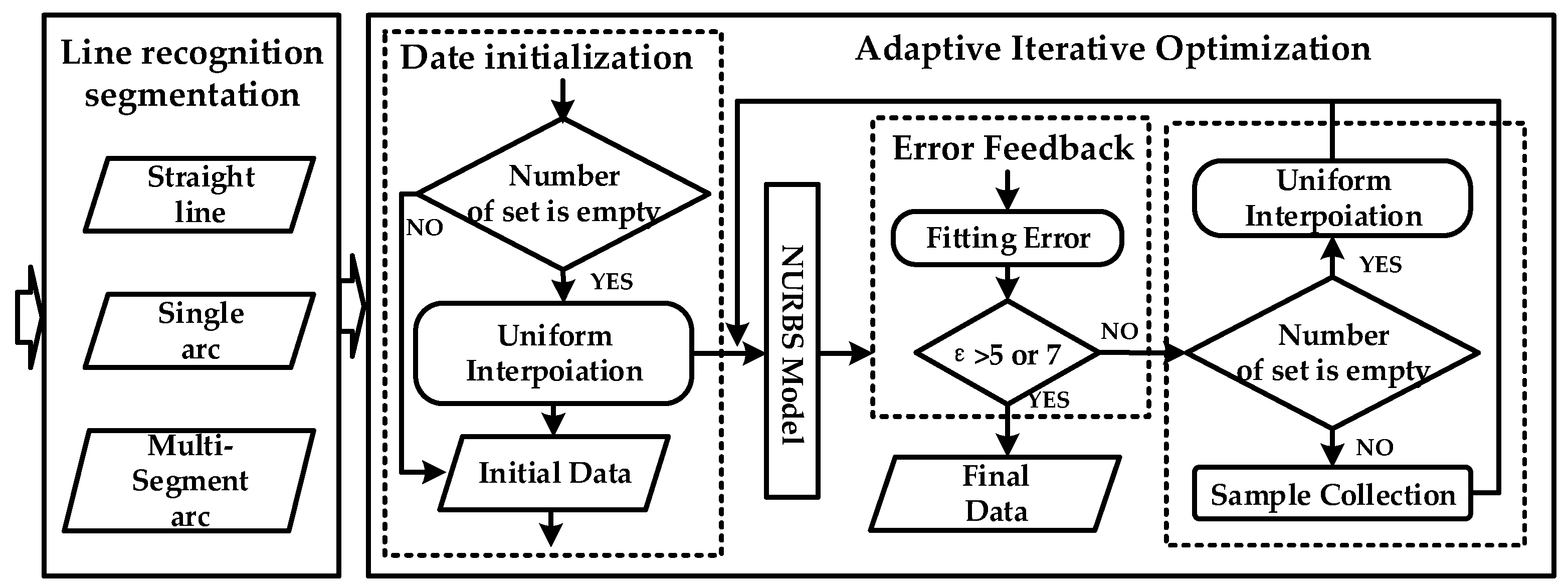
• A memory self-learning strategy is devised based on the cascaded NURBS. This strategy dictates that the input data density is adjusted adaptively and iteratively according to the fitting deviation of the NURBS curve, which reduces the data storage requirements of the lane lines.
• An accurate adaptive dynamic memory curve representation method is developed based on the cascaded NURBS. This method only requires a small data storage volume to ensure that the lane line fitting error meets the requirement.

2. Background and Motivation

2.1. Background

LRMs provide intelligent vehicles with high-precision location information in the real world. One of the key elements of an LRM is the lane line. The highway design standard (JTG D2017) states that a lane line is composed of straight lines, arcs, and buffer curves. Figure 1 shows three real maps. The arcs of the lane line mainly include a single-segment arc (see Figure 1c), a multi-segment arc with consistent tangency direction (see Figure 1a), and a multi-segment arc with inconsistent tangency direction (see Figure 1b). A multi-segment arc with consistent/inconsistent tangency direction is segmented by connection and inflection points into multiple single-segment arcs. The connection and inflection points are represented by “*” in Figure 1c and “×” in Figure 1b, respectively.

The road geometric data obtained from the data acquisition and processing systems are represented by a large number of discrete points. However, this type of geometric representation is not sufficient for constructing a road map with a high storage efficiency. In addition, a point-based representation makes it difficult to extract the required road geometry information, such as the tangent angle and road curvature. In order to solve these problems, it is necessary to fit the road geometry point data using the mathematical modeling technology in order to improve the storage efficiency and availability. In the road-modeling system, it is feasible to either approximate the obtained road geometry data into piecewise parameter polynomials to meet the accuracy and storage efficiency requirements, or use lines and circular arcs, B-spline [2], etc., as a mathematical model of the curve to construct the lane lines.

2.2. Motivation

Lane lines can be modeled and represented using piecewise polynomials, lines and circular arcs, and B-spline [8,16], their comparison is shown in

Table 1. Curve model comparison.

	Smoothness of Segmented Joints	Consistency	Fitting Precision	Memory Efficiency	Convenience/Stability of Modification
Piecewise polynomial	◇	○	◇	◇	◇
Lines/Circular arcs	○	○	◇	◇	○
B-spline	□	□	◇	□	□
NURBS	□	□	□	◇	□

(□: good ◇: general ○: poor).

. The polynomials can be used to approximate the road curves and allow for convenient calculation of the heading angle and lane curvature, but they have a high computational complexity and are not suitable for storing large-scale maps. Lines and circular arcs can represent road curve elements such as lane lines with a small data storage volume, but they cannot guarantee good continuity at the junctions of lines and arcs. B-spline has many excellent properties, such as supporting unified modeling of curves, good smoothness, etc. However, its low accuracy in representing the arcs makes it unsuitable for lane lines that have a large number of arcs. A number of methods can be used to approximate the road lanes, but it is very difficult to make tradeoffs between the model representation accuracy and the data storage volume.

LRMs are supposed to provide accurate location data for intelligent vehicles, which places stringent requirements on the representation models of lane lines and other elements. These include requirements on continuity and ease of calculation in addition to the accuracy and memory efficiency requirements. NURBS is an extension of B-spline. As shown in Figure 2, (a) is a straight line, (b) is an arc, and (c) is a buffer curve, where P_i is the control vertex of NURBS and the black lines are the edges of the control polygon. NURBS is convenient in terms of curve shape modification, data storage, and calculation. They can achieve a high fitting accuracy and, therefore, is suitable to serve as a mathematical model of lane lines and other elements. However, NURBS needs to store a series of weight factors, which is not needed by B-spline. This paper proposes an autonomous storage optimization LRM generation strategy based on cascaded NURBS, which performs iterative optimization according to the error feedback and automatically makes tradeoffs between the error and storage efficiency.

3. Model and Methods

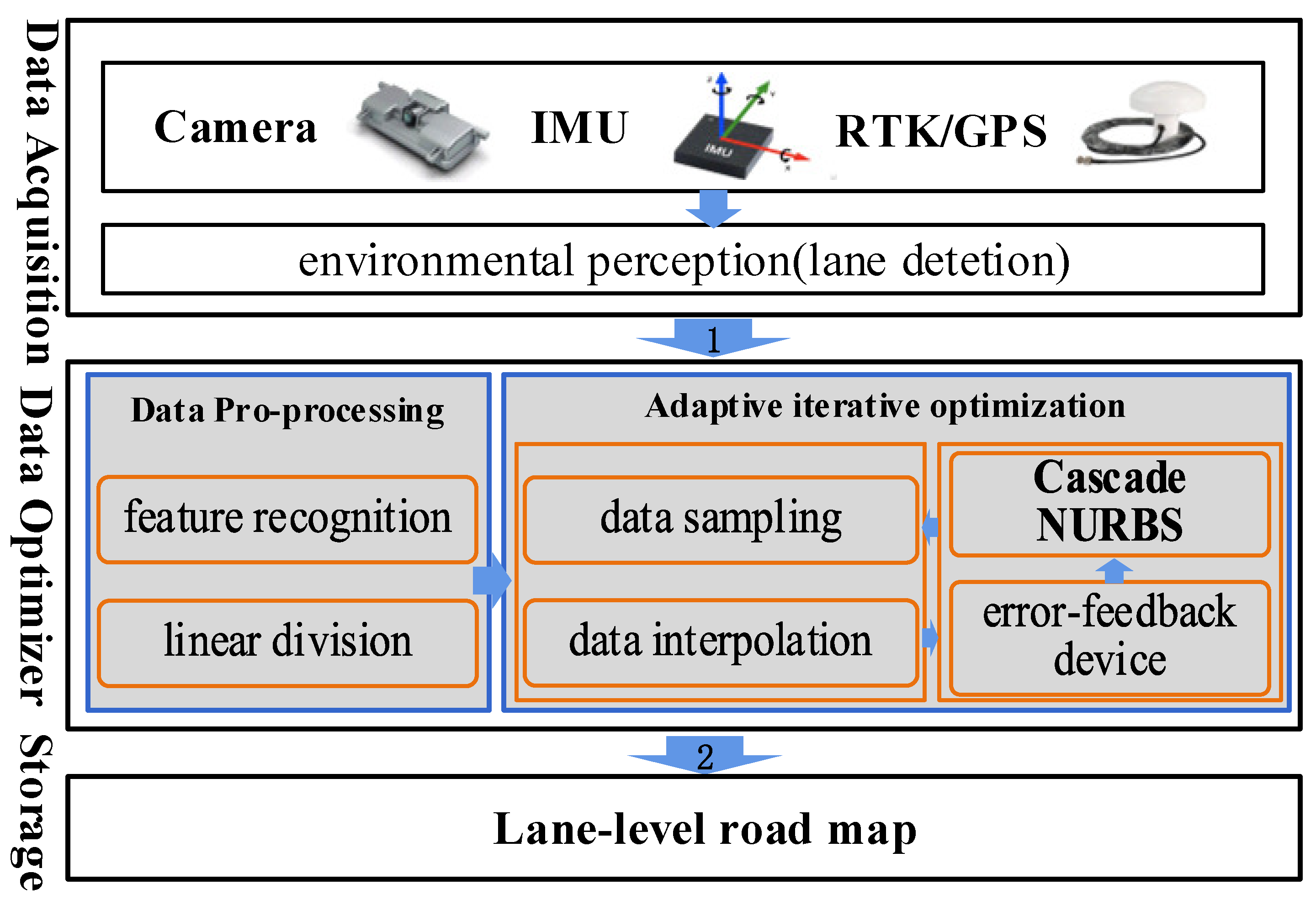
3.1. Overview

We analyzed the lane lines of LRMs and obtained their recursive definition based on the fractal geometry theory. Subsequently, we built a self-learning storage optimization model of this element based on the idea of dynamic programming. An autonomous storage optimization LRM generation strategy based on cascaded NURBS was developed based on the above theoretical analysis and model. The proposed strategy is represented by the data optimizer layer of the frame, as shown in Figure 3, and mainly consists of data preprocessing and an adaptive iteration optimization module. The main framework of LRM generation shown in Figure 3 is divided into three layers: a data acquisition layer, a data optimization layer, and a storage layer. The data-preprocessing module identifies the features of various line shapes hidden within the discrete points of the lane lines. The data optimization layer is used to make tradeoffs between the memory consumption and representation accuracy of the LRM lane lines and other elements and divide them into several segment subsets such as line and arc subsets. The adaptive iteration optimization module iteratively optimizes the memory efficiency of the subsets according to the feedback received from the error feedback device.

The NURBS curve has a powerful freeform description ability and can represent the conic arc uniformly and accurately. A good curve approximation method is based on generating as few curve segments as possible. In this paper, the single-segment and multi-segment arcs with a consistent tangency direction are fitted as a single class, and the multi-segment arc with an inconsistent tangency direction is processed separately.

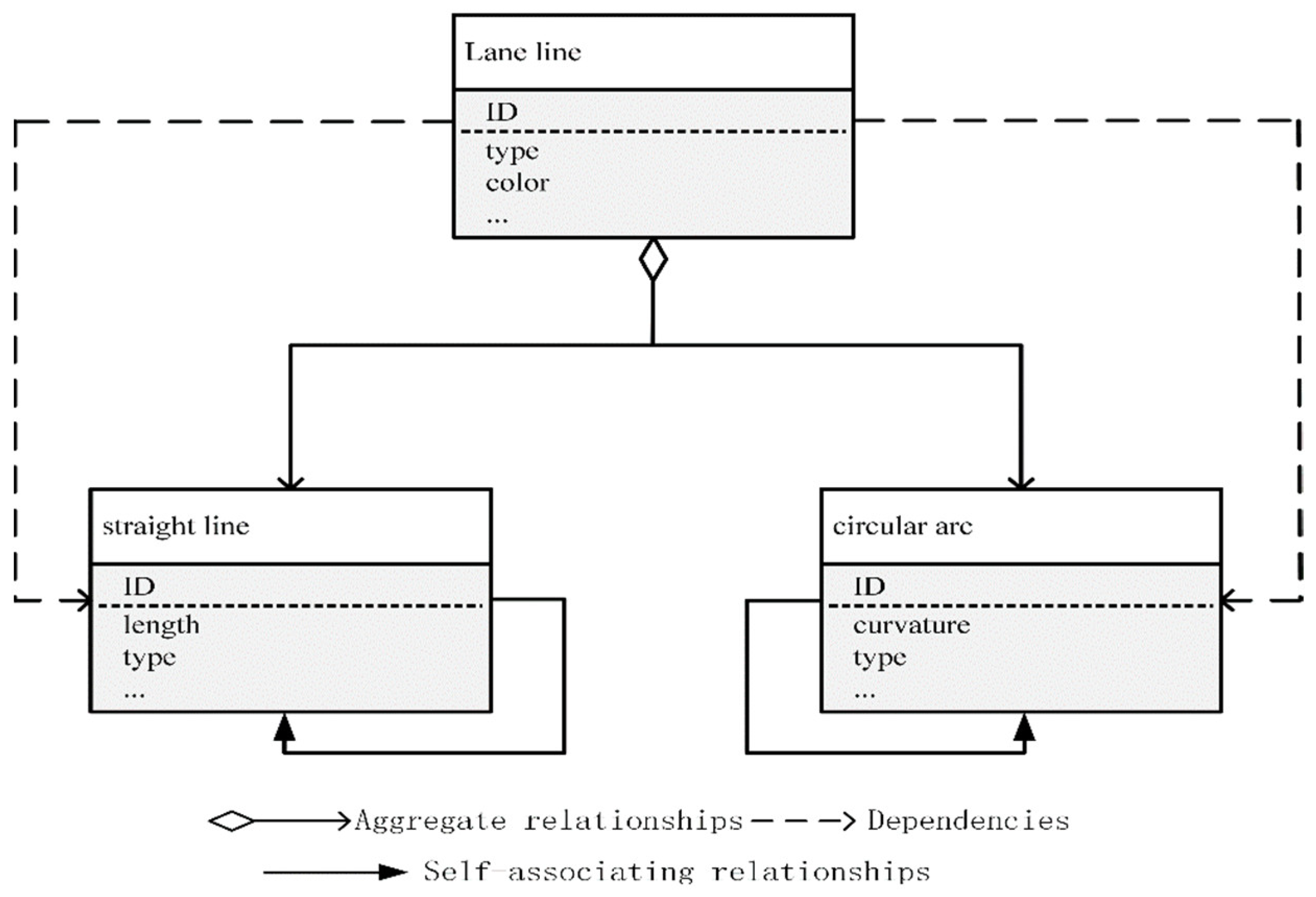
3.2. Lane Line Storage Model

In this section, the recursive definition of a lane line is obtained using the fractal geometry theory. Using the recursive definition, a recursive feedback system model for the storage of LRM lane line elements is constructed based on dynamic programming.

3.2.1. Recursive Definition of Lane Line

A lane line can be abstracted into a geometric object, i.e., a curve composed of straight-line and arc segments. Its recursive definition can be obtained based on the fractal geometry theory: A lane line is composed of meta lane lines, i.e., straight-line and arc segments, and lane lines, as shown in Figure 4. A lane line, straight-line segment set, and arc segment set of the lane line are represented by f (α), g (β), and g (γ), respectively. The definition can be expressed as follows:

$$f\left(\mathit{\alpha }\right)=f\left(\mathit{\alpha }\right)\cup g\left(\mathit{\beta }\right)\cup g\left(\mathit{\gamma }\right)$$

(1)

$$g\left(\mathit{\beta }\right)=g\left({\beta }_1\right)\cup g\left({\beta }_2\right)\cup \dots \cup g\left({\beta }_m\right)$$

(2)

$$g\left(\mathit{\gamma }\right)=g\left({\gamma }_1\right)\cup g\left({\gamma }_2\right)\cup \dots \cup g\left({\gamma }_h\right)$$

(3)

where α = β∪γ and α = {α₁, α₂…α_n|α_i = (x_i, y_i)}, β = {β₁, β₂…β_m}, γ = {γ₁, γ₂…γ_h}, and both β_i and γ_i are sets whose elements are α_i.

The NURBS can provide a unified mathematical expression for lane and meta lane lines. The NURBS curve [9] is expressed as follows:

$$C\left(u\right)=\frac{{{\displaystyle \sum }}_{i=0}^n{w}_i{P}_i{N}_{i,k}\left(u\right)}{{{\displaystyle \sum }}_{i=0}^n{w}_i{N}_{i,k}\left(u\right)},0\le u\le 1$$

(4)

where P_i, (i = 0, 1,…n) is the coordinate value of the i-th control point and $w$ is the weight factor of P_i. The sum of all weight factors should be equal to 1, i.e.,

$${{\displaystyle \sum }}_{i=0}^n{w}_i=1$$

(5)

The weight factors are selected based on the following principle: The selected weight factors should give a second-order geometric continuity to the resulting NURBS curve, ensuring that (1) the connections between segments are smooth enough, and (2) there are no redundant inflection and singular points, i.e., the curvature change is small. In addition, it is necessary to ensure that the first and last weight factors are greater than 0, i.e., w₀ > 0 and w_n > 0.

The cumulative chord-length method is used to perform uniform/non-uniform piecewise sampling/interpolation on the cascaded NURBS numbers. A number of nodes is added in each round of iteration. The sampling or interpolation is uniform for each segment, whereas it is non-uniform for the whole lane line. The calculation involved in the cumulative chord-length method is as follows:

$$d={{\displaystyle \sum }}_{k=0}^n\parallel Q_k-Q_{k-1}\parallel$$

(6)

$$\{ \begin{array}{l}{u}_0=0,u_1=1\hfill \\ \Delta Q_k=\frac{Q_k-Q_{k-1}}{d},k=0,1,2\dots \hfill \\ u_{k+1}=u_k+\Delta Q_k\hfill \end{array}$$

(7)

where u is the node vector, d is the sum of chord lengths between two adjacent points, and $\Delta Q_k$ is the forward difference vector.

3.2.2. Modeling of Recursive Feedback System

The fractal abstraction of the lane line shows that it can be obtained by iteratively combining basic elements (meta lane lines) such as straight-line and arc segments in the same space. Thus, the line can be obtained using a recursive feedback system. In order to get an accurate presentation of a lane line based on cascaded NURBS and ensure the smallest data storage volume within the error constraint, we need to model the recursive feedback system as follows:

$$min\hspace{1em}T\left[f\left(\alpha \right)\right]={{\displaystyle \sum }}_{i=1}^{n}f\left({\alpha }_i\right)$$

(8)

Subject to

$$\{\begin{array}{l}min T\left[g\left({\beta }^{*}\right)\right]\\ \Vert p_j-g\left({\beta }_j^{*}\right)\Vert \le {\epsilon }_1\\ j=1, 2, 3\cdots , m\end{array}$$

(9)

$$\{\begin{array}{l}min T\left[g\left({\gamma }^{*}\right)\right]\\ \Vert p_k-g\left({\gamma }_k^{*}\right)\Vert \le {\epsilon }_2\\ k=1, 2, 3\cdots , h\end{array}$$

(10)

$$\{\begin{array}{l}\Vert p_i-g\left({\gamma }_i^{*}\right)\Vert \le \epsilon \\ i=0, 1, 2, 3\cdots , n\end{array}$$

(11)

where T represents the size of storage space used, and ${\epsilon }_1$ and ${\epsilon }_2$ represent the application errors of straight-line and arc segments, respectively. Equations (9) and (10) are used to calculate the minimum data storage volume of each meta lane line on the premise of meeting the application error requirement, where min T [] is the index function of the meta lane line, i.e., the objective function. The discrete point set α can be divided into meta lane line discrete point sets β and γ according to the spatial characteristics. The numbers of elements in β and γ represent the numbers of straight-line and arc segments contained in the lane line, respectively. Let the state variables be ${\beta }_i^{*}$ (0 < i ≤ m) and ${\gamma }_j^{*}$ (0 < j ≤ h), which contain several elements representing the meta lane lines.

The initial state is given as:

$${\beta }_i^{*}=\varnothing \left(0<i\le m\right),{\gamma }_j^{*}=\varnothing \left(0<j\le h\right)$$

(12)

where ${\beta }_i^{*}$ and ${\gamma }_j^{*}$ respectively meet the following constraints:

$$A{x}_i+B{y}_i+C=0,\left(A\ne 0,B\ne 0\right)$$

(13)

$$A{x}_i^2+B{x}_i{y}_i+C{y}_i^2+D{x}_i+E{y}_i+F=0,\left(A\ne 0,B\ne 0\right)$$

(14)

In addition, the connection points of the meta lane lines satisfy the second-order continuity condition.

Let the decision variable be U. Taking ${\beta }_i^{*}$ as an example, we obtain:

$$U=\{ \begin{array}{l}{\beta }_i^{*}\stackrel{{\alpha }_i}{\leftarrow }\left({\beta }_i^{*}-{\beta }_i\right),\begin{array}{l}\Vert p_i-g\left({\beta }_i^{*}\right)\Vert \ge {\epsilon }_1\hfill \\ \left({\beta }_i^{*}-{\beta }_i\right)\ne \varnothing \hfill \end{array}\\ {\beta }_i^{*}\stackrel{{\alpha }_i}{\leftarrow }interp\left({\beta }_i\right),\begin{array}{l}\Vert p_i-g\left({\beta }_i^{*}\right)\Vert \ge {\epsilon }_1\hfill \\ \left({\beta }_i^{*}-{\beta }_i\right)=\varnothing \hfill \end{array}\end{array}$$

(15)

When the fitting error of the meta lane line, i.e., the straight-line segment, is higher than the application error ${\epsilon }_1$, it is still necessary to update the state variables ${\beta }_i^{*}$ and ${\gamma }_j^{*}$ through decision-making. When the difference set between the state variables ${\beta }_i^{*}/{\gamma }_j^{*}$ and the meta lane line set ${\beta }_i^{*}/{\gamma }_j^{*}$ is not empty, the elements in the difference set are added to the state variables. Otherwise, interpolation is performed on the meta lane line set. The dynamic decision-making process is terminated after the interpolation points are added to the state variables and the error requirement is satisfied. The endpoints of the straight-line segment or circular-arc segment are preferentially selected as the fitted data points, and if the fitting error is larger than the application error, the data points located in the middle of the endpoints are selected from the original data points for interpolation fitting.

The recursive equations are:

$$f_k\left(\mathit{\alpha }\right)=f_{k-1}\left(\mathit{\alpha }\right)\cup g\left(\mathit{\beta }\right)\cup g\left(\mathit{\gamma }\right)$$

(16)

Let the actual application error be δ, and the difference between δ and the set error ε is denoted by $\Delta \delta$. The practical application error decreases as the number of segments increases. The convergeability of the recursive feedback system is proven as follows:

• When $i=1$, $\Delta {\delta }_1=\left|{\delta }_1-\epsilon \right|$;
• When $i=2$, $\Delta {\delta }_2=\left|{\delta }_2-\epsilon \right|$, and $\Delta {\delta }_2<\Delta {\delta }_1$;
• When $i=n$, $\Delta {\delta }_n=\left|{\delta }_n-\epsilon \right|$, and $\Delta {\delta }_n<\Delta {\delta }_{n-1}$;

To sum up, $\Delta {\delta }_1>\Delta {\delta }_2>\cdots >\Delta {\delta }_{n-1}>\Delta {\delta }_n$ and $\underset{i\to n}{\lim }\left|{\delta }_i-\epsilon \right|=0$. The existence of this limit indicates that the number of segments converges on the premise of satisfying the application error requirement. As the data storage volume depends on the number of segments, it can also converge on the premise of satisfying the application error requirement, i.e., there is a feasible solution to Equation (8).

3.3. Autonomous LRM Storage Optimization Method Based on Cascaded NURBS

This section describes the fractal that converts lane lines into meta lane lines. Furthermore, the autonomous storage optimization strategy based on cascaded NURBS for constructing a recursive feedback system is elaborated.

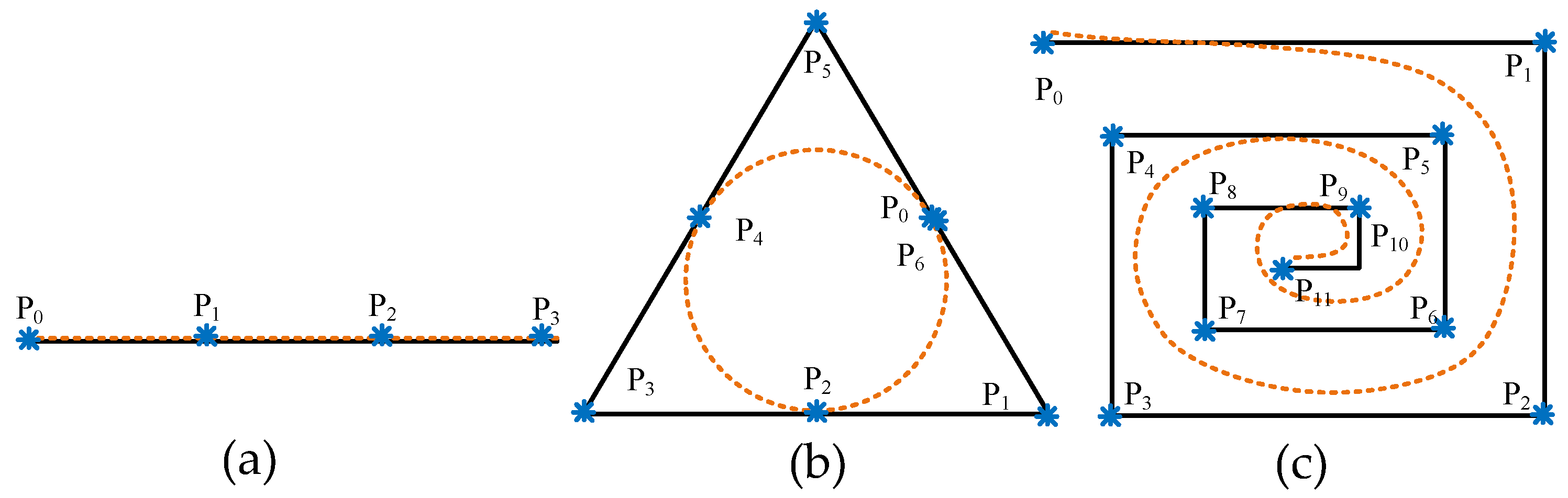
3.3.1. Random Shape-Dividing Algorithm of Lane Lines

A lane line is transformed into an equivalent set of meta lane lines using the fractal. Thus, the original lane line is divided into straight-line and arc segments. In this paper, the single-segment and multi-segment arcs with a consistent tangency direction are fitted as a single class. Line shape feature identification and division are performed on the data point set D, which contains road curve information such as lane lines. The identification and division method can be seen in the pseudocode of Algorithm 1.

The original data set is divided into three subsets: (1) straight line subsets, represented by “linear”; (2) the subset of single-segment and multi-segment arcs with a consistent tangency direction, represented by “circular”; and (3) the subset of multi-segment arcs with an inconsistent tangency direction, represented by “multicircular”.

In the second line of the algorithm, the input data points d_i are utilized to calculate the coordinates of the circle center $C_i$ and the radius $R_i$. If d_i belongs to the current arc, then $r_i\to \infty$. In this paper, $R_{\max }$ represents an infinitely large number. Lines 3–13 of the algorithm are used to identify and divide the data points on the straight-line and arc segments according to the radius. In lines 6–10, the algorithm distinguishes the endpoints of single-segment and multi-segment arcs based on whether the current circle center resides within the circle calculated last time.

Algorithm 1 Lane Line Ungauged Fractal Algorithm

Input: D, Rmax

Output: map

1. for (i = 1; i < size(D); i++) do

2. [Ci, ri] = point2circle(di);

3.  if (ri > Rmax) then

4.   map(j).type = ‘linear’; map(j).data = [Ci,ri];

5.  else

6.   map(j).type = ‘circle’; map(j).data = [Ci,ri];

7.   if (map(j).data > 1) then

8.    dis = sqrt(pow(x − Ci.x)+ pow(y − Ci.y));

9.   end

10.   if (dis > pow(ri)) then

11.    map(j).type = ‘mulcircular’;

12.   end

13.   if (the type is different) then

14.    j = j + 1;

15.  end

16. end

17. end

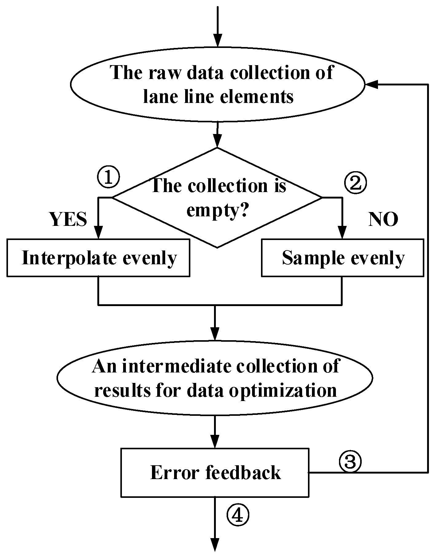
3.3.2. Error Feedback LRM Storage Self-Optimization Method Based on Cascaded NURBS

The NURBS curve has different degrees of control for the straight line and arc; therefore, it is impossible to achieve the overall goal of optimal minimization of the data storage volume within the application error constraint using the same fitting error standard and data-sampling method. In the method proposed in this paper, iterative sampling, curve fitting, and error processing of data points are performed for different types of meter lane lines, where the original data point set within the specified error limit is approximated with the goal of minimizing the overall data storage volume.

The purpose of data preprocessing is to identify and divide the lane line dataset according to the line shape, obtaining multiple sets of meta lane lines. In order to ensure the continuity between different segments, the initial datapoint set of each segment must include the first and last endpoints of the segment datapoint set. Figure 5 shows the logic of the iterative sampling based on the error feedback device.

All meta lane lines are represented using three-time NURBS modeling. A section of p-th order NURBS needs at least p + 1 control points. A minimum of four points is required for a straight-line segment; therefore, the initial resulting datapoint set of the straight-line segment should include the first endpoint, last endpoints, and two intermediate points of the original data set of the segment. For an arc segment, the initial result datapoint set of a single-segment arc includes the first and last endpoints, as well as five intermediate points in the original data set. A multi-segment arc with a consistent tangency direction is divided into n single-segment arcs through several connection points, which are the endpoints of the single-segment arcs. Therefore, the initial resulting datapoint set of a multi-segment arc with a consistent tangency direction includes the initial datapoint sets of n single-segment arcs. Similarly, a multi-segment arc with an inconsistent tangency direction is divided into multiple single-segment arcs using several inflection points; thus, the same sampling scheme is used to compile the initial resulting datapoint set.

After NURBS curve fitting is performed each time according to the sampled datapoints, the deviation ε between the original datapoint set $p=\left\{p_1,p_2,\dots p_n\right\}$ and the generated curve C (u) can be calculated as follows:

$$\epsilon =max\Vert p_i-C\left(u_i\right)\Vert ,i=0,1,\cdots n$$

(17)

The reasonable fitting error of the straight line/arc is set to 5/7 cm. When ε < 5/7 cm, the unselected data in the original data set are selected and added to the resulting datapoint set, which increases the number of nodes in the interval. The iteration will be terminated when ε reaches a value equal to or greater than 5/7 cm, as shown by ③ and ② in Figure 5, which determines the resulting datapoint set of sampling the current straight-line segment. In this way, additional control points are obtained by inserting nodes to increase the flexibility of curve shape control.

If it is not possible to always meet the error constraint requirement, uniform equidistant interpolation should be performed on the resulting data set to increase the node density in the interval, as shown by ① in Figure 5. This process is continued until a resulting datapoint set that meets the error requirement is obtained, as shown by ④ in Figure 5.

4. Experiment and Discussion

4.1. Setup and Implementation of Experiment

The real vehicle used to acquire data was equipped with a high-definition camera and high-precision RTK/GPS + INS equipment. High-accuracy vehicle attitude data were obtained by combining GPS and INS data, and an accurate lane line data set was obtained by performing perception and solution operations using the perception algorithm. The experimental data processing and simulation program was executed on a 64-bit PC with Intel Core i7 7th Gen CPU and 8 GB RAM. The MATLAB 2021a environment was used for running the data processing and experiment programs.

The NURBS toolbox and Math toolbox in MATLAB were used to inversely obtain the NURBS control points, calculate the distance from the point to the curve, and evaluate the storage efficiency with the help of performance and memory usage. The cumulative chord-length method was used to sample or interpolate the data.

Figure 6 shows the data-processing procedure for adaptive iteration optimization. The obtained lane line position data were preprocessed at first by using Algorithm 1 to divide the original data set into several subsets of straight lines and arcs. Subsequently, NURBS was used to iterate on the above data subsets for the data fitting and deviation calculation that was performed on the subsets. Finally, the original data were sampled or interpolated according to the deviation until the application error requirement was met. The piecewise iteration process can be accelerated by using parallel computation.

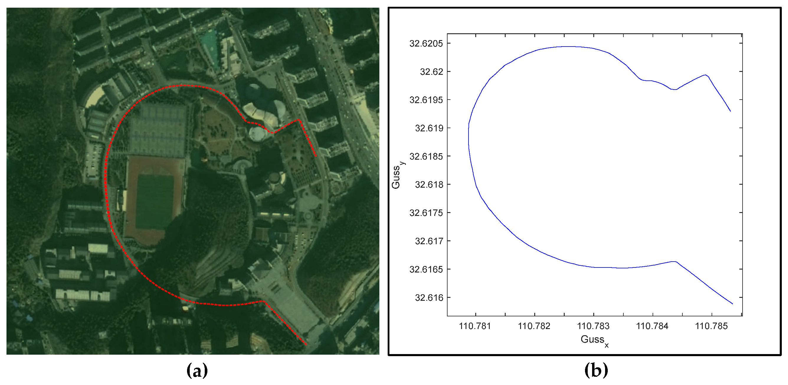
4.2. Data Acquisition and Processing

A real vehicle equipped with the equipment and the perception module of the real vehicle was used to acquire the real road data of an industrial park. Figure 7a,b shows the route taken in the experiment and the dataset visualization, respectively. The length of the route related to the dataset was 926 m. The acquired data were abstracted into a single lane. The real route is shown as the red curve in Figure 7a, and the visualization of the acquired real dataset is shown as the blue curve in Figure 7b.

4.3. Lane Model

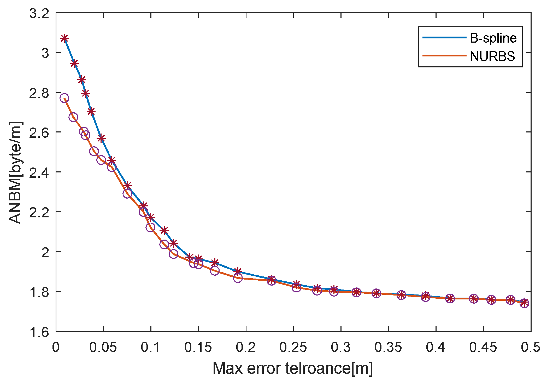
• Memory Efficiency

We evaluated the storage efficiency of the proposed method by using the proposed method and the B-spline modeling method [4] to separately model a lane line in the obtained dataset, as shown in Figure 7. The data storage demand of the NURBS curve mainly came from the control points (two floating-point numbers) and weight factor (an integer). Assuming that each floating-point number needs four bytes and each integer needs one byte, the average number of bytes per meter (ANBM) is defined as follows:

$$ANBM=\frac{2\times m\times 4byte+m\times 1byte}{L}$$

(18)

where L is the total length of lane line, and m is the number of control points/weight factors. Figure 8a shows the control points formed by using original data points of the lane line as input.

The method proposed in this paper was used to process the original data points, and the resulting data points for fitting the lane line are shown in Figure 8b, where the blue curve is the final fitted lane line. Thanks to the implementation of the proposed method, the data volume decreased significantly while meeting the error requirement of autonomous vehicles, i.e., the fitting error was less than 0.1 m. Figure 8 shows the adaptive iteration memory optimization process. Initially, the proposed method took samples according to the minimum data storage volume. If the fitting error did not meet the requirement, the method increased the data density and performed fitting again. Therefore, the data storage volume increased as the fitting error decreased. The ANBM was inversely proportional to the error tolerance.

Figure 9 compares the memory efficiencies of the proposed method and the B-spline curve model under C¹ continuity. It can be observed that the proposed method effectively improved the memory efficiency, because it iteratively optimized it in an adaptive manner according to the fitting error requirements defined in different scenes. In the application error range of 0 m–0.1 m, the method in this paper saved an average of 0.17 byte of storage per meter.

• Accuracy

One important goal of LRM systems in terms of accuracy is to generate a mathematical model such that the distance error between lane data points and curves does not exceed the preset tolerance of 0.1 m. Figure 10 compares the fitting errors of the proposed method and the B-spline curve model under the same data storage volume constraint. The sections of abscissa between 0–500 and 3000–3500 correspond to the straight-line segments, whereas the remaining sections correspond to the arc curves. As shown in Figure 10, the maximum error of the method described in this paper was 0.09021 m, the average error was 0.03703 m, and the standard deviation was 0.02667, whereas the maximum error produced by the fit of the B-spline method was 0.11 m, the average error was 0.052092 m, and the standard deviation was 0.03226. In contrast, the fitting accuracy of the method described in this paper was higher. Under the same data storage volume, the two methods exhibited identical fitting performance in the straight-line segments, whereas the proposed method achieved a higher fitting accuracy in processing the arc curves. On the whole, the proposed method had better fitting performance and higher fitting accuracy.

5. Conclusions

In this study, we analyzed road lanes based on the fractal geometry theory and the idea of dynamic programming, derived a lane line storage model, and proved the convergence of the optimization constraint equation. We further devised a framework of accurate curve presentation using adaptive and dynamic memory optimization based on cascaded NURBS. The proposed method could automatically achieve tradeoffs between error and memory efficiency by performing iterative optimization according to the error feedback. Furthermore, it could efficiently store curve elements like lane lines within the fitting error constraint. Our main contribution in this paper was an adaptive storage efficiency optimization strategy based on cascaded NURBS (uniform/non-uniform coupled sampling) and an error feedback device. The cascaded NURBS could uniformly model lane lines of any shape in the real world, and its wide applicability in two-dimensional and three-dimensional spaces and high fitting accuracy were highly helpful in maximizing the storage efficiency. However, this paper needs to obtain the raw data of standardized roads in advance in order to perform storage optimization, and also does not fully consider the real-time online optimization of storage efficiency and non-standardized roads. The results of a simulation experiment carried out on a dataset obtained from a park showed that the proposed method could achieve high accuracy and storage efficiency. Under the constraint of a 0.1 m curve-fitting error, the average memory demand of the lane line elements was less than 2.4 bytes/m.

References

- Kim, D.; Chung, T.; Yi, K. Lane map building and localization for automated driving using 2D laser rangefinder. In Proceedings of the 2015 IEEE Intelligent Vehicles Symposium (IV), Seoul, Korea, 28 June–1 July 2015; pp. 680–685. [Google Scholar]
- Gwon, G.-P.; Hur, W.-S.; Kim, S.-W.; Seo, S.-W. Generation of a Precise and Efficient Lane-Level Road Map for Intelligent Vehicle Systems. IEEE Trans. Veh. Technol. 2016, 66, 4517–4533. [Google Scholar] [CrossRef]
- Yu, Z.; Zhu, H.; Lin, L.; Liang, H.; Yu, B.; Huang, W. Laser Data Based Automatic Generation of Lane-Level Road Map for Intelligent Vehicles. arXiv 2020, arXiv:2101.05066. [Google Scholar]
- Stannartz, N.; Theers, M.; Llarena, A.; Sons, M.; Kuhn, M.; Bertram, T. Comparison of Curve Representations for Memory-Efficient and High-Precision Map Generation. In Proceedings of the 2020 IEEE 23rd International Conference on Intelligent Transportation Systems (ITSC), Rhodes, Greece, 20–23 September 2020; pp. 1–6. [Google Scholar] [CrossRef]
- Vatavu, A.; Danescu, R.; Nedevschi, S. Environment perception using dynamic polylines and particle based occupancy grids. In Proceedings of the 2011 IEEE 7th International Conference on Intelligent Computer Communication and Processing, Cluj-Napoca, Romania, 25–27 August 2011; IEEE: New York, NY, USA, 2011; pp. 239–244. [Google Scholar]
- Betaille, D.; Toledo-Moreo, R. Creating Enhanced Maps for Lane-Level Vehicle Navigation. IEEE Trans. Intell. Transp. Syst. 2010, 11, 786–798. [Google Scholar] [CrossRef]
- Schindler, A.; Maier, G.; Janda, F. Generation of high precision digital maps using circular arc splines. In Proceedings of the 2012 IEEE Intelligent Vehicles Symposium, Madrid, Spain, 3–7 June 2012; IEEE: New York, NY, USA, 2012; pp. 246–251. [Google Scholar]
- Jo, K.; Sunwoo, M. Generation of a Precise Roadway Map for Autonomous Cars. IEEE Trans. Intell. Transp. Syst. 2013, 15, 925–937. [Google Scholar] [CrossRef]
- Jo, K.; Lee, M.; Kim, C.; Sunwoo, M. Construction process of a three-dimensional roadway geometry map for autonomous driving. Proc. Inst. Mech. Eng. Part D J. Automob. Eng. 2016, 231, 1414–1434. [Google Scholar] [CrossRef]
- Guo, C.; Kidono, K.; Meguro, J.; Kojima, Y.; Ogawa, M.; Naito, T. A Low-Cost Solution for Automatic Lane-Level Map Generation Using Conventional In-Car Sensors. IEEE Trans. Intell. Transp. Syst. 2016, 17, 2355–2366. [Google Scholar] [CrossRef]
- Chen, A.; Ramanandan, A.; Farrell, J.A. High-precision lane-level road map building for vehicle navigation. In Proceedings of the IEEE/ION Position, Location and Navigation Symposium, Indian Wells, CA, USA, 4–6 May 2010; pp. 1035–1042. [Google Scholar] [CrossRef]
- Brummer, S.; Janda, F.; Maier, G.; Schindler, A. Evaluation of a mapping strategy based on smooth arc splines for different road types. In Proceedings of the 16th International IEEE Conference on Intelligent Transportation Systems (ITSC 2013), The Hague, The Netherlands, 6–9 October 2013; IEEE: New York, NY, USA, 2013; pp. 160–165. [Google Scholar]
- Barnea, S.; Filin, S. Segmentation of terrestrial laser scanning data using geometry and image information. ISPRS J. Photogramm. Remote Sens. 2013, 76, 33–48. [Google Scholar] [CrossRef]
- Meyer, A.; Walter, J.; Lauer, M. Fast Lane-Level Intersection Estimation using Markov Chain Monte Carlo Sampling and B-Spline Refinement. In Proceedings of the 2020 IEEE Intelligent Vehicles Symposium (IV), Las Vegas, NV, USA, 19 October–13 November 2020; pp. 71–76. [Google Scholar] [CrossRef]
- Piegl, L.; Tiller, W. The NURBS Book; Springer: Berlin/Heidelberg, Germany, 1995. [Google Scholar]
- Reinoso, J.F.; Moncayo, M.; Ariza-López, F.J. A new iterative algorithm for creating a mean 3D axis of a road from a set of GNSS traces. Math. Comput. Simul. 2015, 118, 310–319. [Google Scholar] [CrossRef]