1. Introduction
The stochastic differential equation (SDE) has been used to model various phenomena and investigate their properties, such as the moments, variance and conditional moments, which are beneficial for estimating parameters that play significant roles in several practical applications. For example, financial derivative prices, such as moment swaps, can be obtained by calculating the conditional moments of their payoffs under the risk neutral measure; see for more concrete studies Araneda et al. [
1], Cao et al. [
2], He and Zhu [
3] and Nonsoong et al. [
4]. Actually, such moments can be directly computed by employing SDE’s transition probability density function (PDF). However, the transition PDF is often unavailable in closed form; so is the formula for those conditional moments of the SDE. Investigating properties of those SDEs is still imperative and challenging.
There are several empirical studies confirming that a mean-reverting drift process, such as the Vašíček, Ornstein–Uhlenbeck (OU) [
5] and Cox–Ingersoll–Ross (CIR) [
6] processes, should not necessarily be linear. Indeed, the behaviors and dynamics of interest rate and its derivatives prefer nonlinearity in the mean-reverting drift rather than linear drift processes; see for more details in [
7,
8,
9,
10]. In order to extend the OU process, a nonlinear diffusion process was introduced by Cox [
11], namely, the constant elasticity of variance (CEV) process. The CEV process is useful and has many applications in various fields. However, the drift term of Cox’s CEV process is still linear. For many reasons described in the existing literature [
7,
8], an extended case of Cox’s CEV process was first studied by Marsh and Rosenfeld [
12]. The process is sometimes called the Marsh–Rosenfeld (MR) process, and its transition PDF that can be straightforwardly calculated by using Itô’s lemma and the transition PDF of the CIR process are very complicated; the closed-form formula for conditional moments of the MR process is also complicated or unavailable in general; see for more details in [
13]. It gets even more complicated for an inhomogeneous-time MR process that extends the MR process by replacing the constant parameters in the process with time-dependent functions. From now on, we subsequently call the inhomogeneous-time MR process in general an inhomogeneous nonlinear drift constant elasticity of variance (IND-CEV) process.
Conditional moments have been extensively used in modern financial markets. For example, they can be used to price moment swaps. Unfortunately, the conditional moments, which can be directly computed by applying the transition PDFs, are often unavailable in closed form because the transition PDFs are hardly known. The Feynman–Kac technique is used to overcome this problem for calculating the conditional moments of many stochastic processes. There has still been little research on the analytical formula for conditional moments regarding the IND-CEV process. In this work, a novel approach is developed based on the Feynman–Kac theorem, where the partial differential equation (PDE) is solved analytically, and some combinatorial techniques are used to simplify the system of recursive ordinary differential equations (ODEs) associated with the conditional moment.
The rest of the paper is organized as follows.
Section 2 provides an overview of the IND-CEV process and sufficient conditions of the time-dependent parameter functions in the process. The key methodology and main results are given in
Section 3.
Section 4 proposes some essential properties such as conditional moments, conditional variance and central moments, conditional mixed moments, conditional covariance and correlation.
Section 5 provides the formula of the unconditional moments of the IND-CEV process with constant parameters. Experimental validations for our results applied with Monte Carlo (MC) simulations are addressed in
Section 6. Conclusions, limitations and future researches are discussed in
Section 7.
2. IND-CEV Process
This section presents the IND-CEV process and sufficient assumptions for the process in order to have a unique positive solution. The dynamics of the short-term interest rate over time are assumed to follow the SDE:
with the initial condition
, where
and
are smooth and bounded time-dependent parameter functions and
is a standard Brownian motion, which has asymmetric sample paths, under a probability space
with filtration
. In this study, we only focus on the case that
in the SDE (
1). Let
. Henceforth, the dynamics of the process
are considered via the following SDE:
where
The process
in (
2) is called an IND-CEV process. In addition, the SDE (
2) is called the extended Cox–Ingersoll–Ross (ECIR) process when
; see for more details in [
14,
15,
16,
17]. From (
2), if the parameters
and
are constants written by
,
and
, respectively, then the SDE (
2) can be rewritten as:
where
We will consider SDEs (
2) and (
3) on a time domain
.
We first discuss the solution of SDE (
2).
Assumption 1. The parameter functions and in SDE (2) are strictly positive and continuously differentiable on . Moreover, is locally bounded on . Assumption 2. for all .
Theorem 1. For SDE (2), if Assumptions 1 and 2 hold with , then there exists a pathwise unique strong solution process for all . Proof. Transforming
with the Itô lemma yields:
where
,
and
Thus,
is an ECIR process. Under Assumptions 1 and 2, the functions
,
and
are strictly positive, smooth and continuous time-dependent parameter functions on
. Additionally, we have that:
By the Feller condition [
18], the SDE (
2) has a pathwise unique strong solution in which
avoids zero almost surely under measure
for all
and so does
. □
From now on, we will always assume Assumptions 1 and 2 with .
3. Main Results
In this section, we give the closed-form formula of conditional moments of processes (
2) and (
3). Applying the Feynman–Kac technique and assuming a special form of the conditional moment, we can express the solution of the resulting PDE as an infinite series and solve the system of recursive ODEs to obtain coefficients for the closed-form formula. The results for some special cases are also displayed.
In this work, under the probability measure
and
field
, we first propose the integral-form formula for the conditional moment of an IND-CEV process for
:
for all
and
. Obviously,
. The key idea involves a system with a recurrence differential equation that brings about the PDE by involving an asymmetric matrix. The form of PDE’s solution associated with the conditional moment (
4) is a polynomial expression motivated by [
16,
17,
19,
20,
21,
22,
23,
24]. Hence, we can solve its coefficients to obtain a closed-form formula directly.
Theorem 2. Let be an IND-CEV process satisfying (2). Assume that the conditional moment can be expressed in the form:in which the infinite series uniformly converges on. Then, the coefficients in (5) can be expressed recursively by:for all, where: Proof. Applying the Feynman–Kac formula to the SDE (
2), we have that the function
satisfies the PDE:
for all
and
, with the initial condition:
From (
5),
. Comparing this with (
10) implies that
and
for all
. Substituting (
5) into (
9), we have that:
or it can be simplified as:
Under the assumption that the solution is in the form (
5) over
, this equation can be solved through the system of ODEs:
with initial conditions
and
for
. Hence, the coefficients in the infinite series (
5) can be directly acquired by solving the system (
11), which turns out to be the recursive relation given in (
6). □
Note that when we define variables or notations using the
sign, e.g., Equations (
6)–(
8), we will use those variables or notations throughout this work.
Observe that (
5) becomes a finite sum when one of the two factors for
in (
8) is zero. For fixing
, we give the consequence of (
5) in Theorem 2 when
. The infinite sum in (
5) is cut off at a finite order and can be presented as in the following corollary.
Corollary 1. Let be an IND-CEV process satisfying (2). For the positive real number γ such that , the conditional moment is explicitly given by:for all . Proof. From (
8), when
, we acquire that
. From (
6), the coefficients
for all integers
. Hence, the infinite sum (
5) is actually just the finite sum (
12). Since any integration of a continuous function over a compact set is finite, the finite sum (
12) exists for all
; hence, the infinite sum (
5) uniformly converges to the finite sum (
12) and
. □
Another consequence of (
5) in Theorem 2 is shown in the following corollary.
Corollary 2. Assume that follows SDE (2) and there exists such that:for all . Then,for all . Proof. From (
8), when
, we have that
. From (
6), the coefficients
for all integers
. With the same reasoning as in the proof of Corollary 1, we acquire the desired result. □
One main concern when we investigate the conditional moments described by the IND-CEV process is that the integral terms (
6) in Theorem 2 cannot be directly evaluated. Thus, a very accurate numerical integration scheme is applied via the Chebyshev integration method; see [
25,
26,
27,
28] for more details.
Next, we consider the case when and are constant functions.
Theorem 3. If follows the SDE (3) and the conditional moment can be expressed in the form (5), then the conditional moment is given by:for all , where:Note that the product from 0 to , , is defined to be 1. Proof. We will prove by induction that:
for all
. From (
6) with the constant parameters
,
and
, we have that
and
for all
. By substituting
in (
17), we obtain:
Let
. Assume that:
From (
17), we have that:
□
From Corollaries 1 and 2, when and are constant functions, we have the following corollaries.
Corollary 3. Assume that follows SDE (3). For a positive real number γ such that , the conditional moment is explicitly given by:for all . Note that the product of in (18) for is defined to be 1. Corollary 4. Assume that follows the SDE (3). If there exists such thatthenfor all . For SDE (
3), characterization for the convergence of the series (
15) can be provided.
Theorem 4. Assume that follows SDE (3) and for all . Then, the series (15) diverges for all . Proof. Since
for all
, we have that
and
for all
.
The above expression is
as
; hence, the limit diverges. By ratio test, the series (
15) diverges for all
. □
From Corollaries 3 and 4, and Theorem 4, we have the following result.
Corollary 5. Assume that follows SDE (3). Then, the series (15) converges for all if and only if: The convergent results for case 1 and 2 are given in Corollaries 3 and 4, respectively.
4. Probabilistic Properties
This section illustrates some usefulness of our results from
Section 3 including the first, second and fractional conditional moments; conditional variance and central moments; conditional mixed moments; and conditional covariance and correlation.
Example 1 (The conditional moments).
From Corollary 1, the conditional moment of an IND-CEV process when the parameter for some is given by: where: for , where: For constants κ, θ and σ, we use and in Corollary 3. Then, for , the first and second conditional moments are given by: and For , the first and second conditional moments are given by: and Additionally, for , the conditional moment with is given by: Next, we propose the consequences of Example 1, which are the conditional variance and central moments, conditional mixed moments, and conditional covariance and correlation, as follows.
Example 2 (The conditional variance and
central moment).
By applying Corollary 3, (21) and (22), the conditional variance of the IND-CEV process can be given by: where and are derived in (21) and (22) for the CIR process. In general, the central moment is presented by: where . Example 3 (The conditional mixed moments).
By applying the tower property for where and and Corollary 1, the conditional mixed moment of the IND-CEV process (2) with is given by: In addition, the general formula for conditional mixed moments , where and , for the process (3) can be analytically derived by using Corollary 3. Example 4 (The conditional covariance and correlation).
The conditional covariance of the CIR process for where and is given by: Applying the results from (26) and (27), we obtain that the conditional correlation of the CIR process is given by: We can generalize (27) and (28) by using (26) as the closed forms of and , where and are positive integers. 5. Unconditional Moments of the IND-CEV Process
This section provides the formula of the unconditional moments of the IND-CEV process with constant parameters as reduced from the formula of conditional moments.
Theorem 5. Assume that follows SDE (3). Then, for all Proof. Let
. By considering (
18) in Corollary 3, the coefficient terms of
converge to 0 as
for
. Thus, the summation (
18) is reduced to only one term, where
,
where
is defined in (
16). By expressing
to the above equation, it can be performed to
□
Note that the formula for unconditional moments does not rely on the initial value
r, and these unconditional moments represent the moments of the stationary distribution of the process (
3).
6. Experimental Validation
In this section, we validate the closed-form formulas presented in Theorem 2 and Corollaries 1 and 2. The Euler–Maruyama (EM) method was applied to simulate the process (
2) and approximate the conditional moments based on the symmetry concept. For an interval
, let
for a fixed
and
for
. We denote a numerical solution of the IND-CEV process at time
by
. The EM approximation of (
2) on the interval
is defined as
and
where
are
N independent standard normal random variables. In this validation, the MC simulations based on the EM method (
30) were conducted by MATLAB R2021a software on a quadcore Intel Core i5-1035G1 with 8 GB RAM.
Example 5. In this example, we apply the MC simulations based on the CEV process [15]:where κ andare positive constants,is a non-negative constant and d is a positive integer greater than 2. By considering (31) and (2), the parameter functions for SDE (31) areand. Note that Assumptions 1 and 2 hold for these parameter functions. By Theorem 2, we have that:where:However, Formula (32) can be reduced to a finite sum for a particular situation. By Corollary 1, if, then:By Corollary 2, if there existssuch that, which isin this example, for all, then: Our experiments are classified into three cases: (i) , (ii) , and (iii) and . The algorithm of our validation is given in Algorithm 1. The parameters , , and in the process (31) are set for all of these three cases. MC simulations were performed at each initial value and .| Algorithm 1 MC validation for the process (31) |
- 1:
Set the values for parameters
|
- 2:
|
- 3:
Compute according to ( 33) for a refined grid of variables r and τ
|
- 4:
Plot a surface of representing the conditional moments from our formulas
|
- 5:
Construct a grid of variables r and τ to perform MC simulation
|
- 6:
For each initial value r and final time τ, apply the EM method with 1000 time steps to the process ( 31) to get with 1000 sample paths and compute the average value of
|
- 7:
Plot the resulting values and compare them with the surface of
|
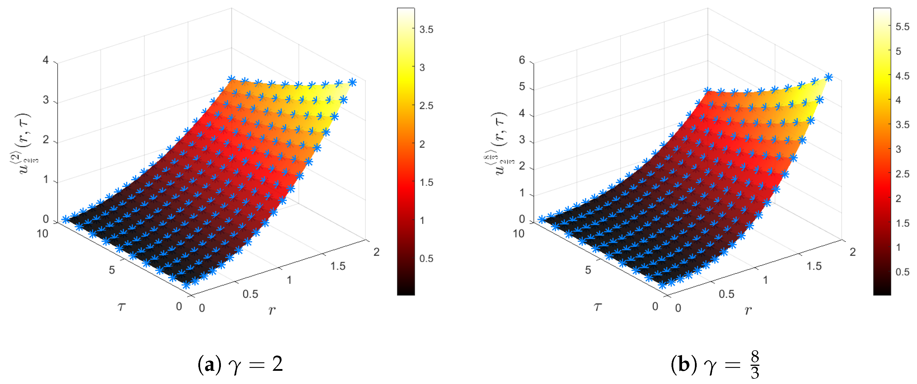
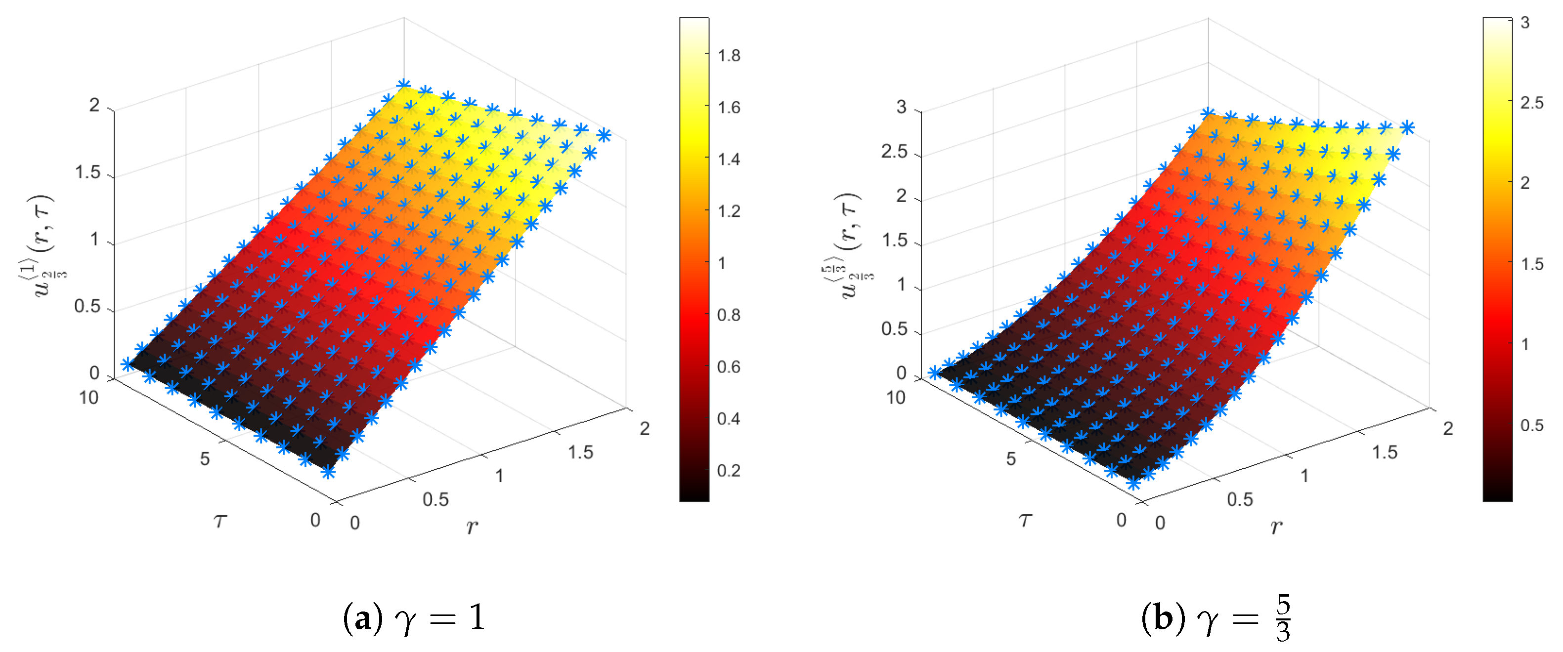
For the case when, we setand consider two different values of γ. Here, we chooseand. Figure 1 shows the comparison between Formula (34) and MC simulations. The results from MC simulations are presented by blue star markers, and Formula (34) is presented by the solid surfaces. All markers perfectly match with the surfaces. This indicates that our formula from Corollary 1 is correct. The validation runtimes forandwere and
s, respectively. For the case when, we setand considerand. Figure 2 demonstrates the comparison between Formula (35) and MC simulations. Evidently, the results from MC simulations and the surfaces from Formula (35) are completely coincident. Validation runtimes for and
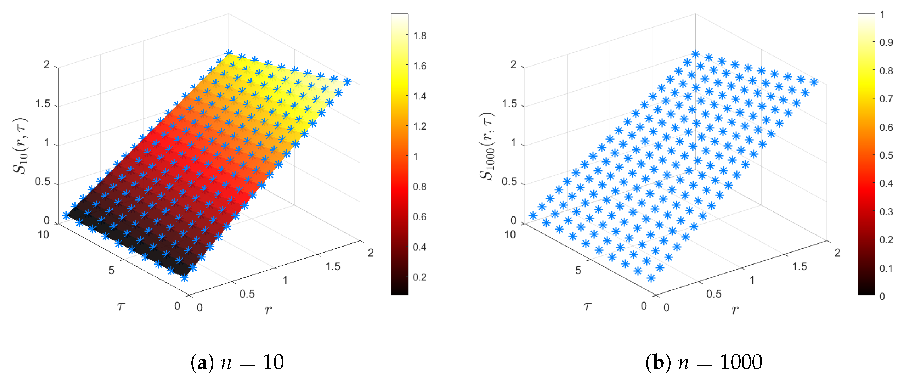
were 22.34 and 22.63 s, respectively. For the case whenand, we setand consider. Observe that from (
33),
is
as
; thus, for . By the ratio test, the summation diverges; hence, Formula (32) diverges for all . This means that the conditional moment cannot be expressed in the form (5). However, our experiment shows that finite terms of the summation in Formula (32) can be used to approximate the conditional moment. Figure 3 shows the comparison between the formula for and MC simulations. The results from MC simulations coincide with the surface from Formula (36) with . For
, the results from Formula (36) could not be computed by our machine. This supports our theory that Formula (32) diverges. Validation runtimes for and
were
and
s, respectively. The next example shows a similar result of the third case in Example 5 for the IND-CEV process with constant parameter functions.
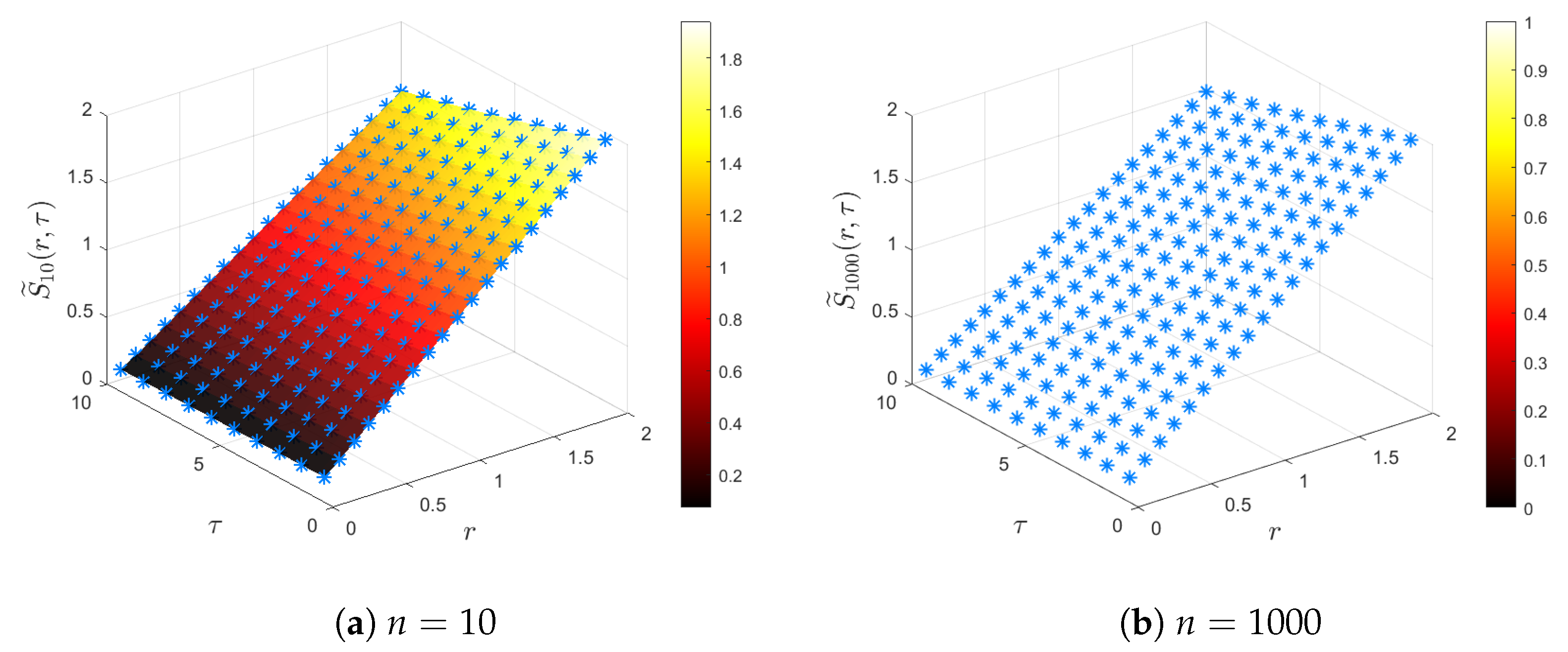
Example 6. For SDE (3) with , , , , and , we have that and . From Corollary 5, cannot be expressed in the form (5). However, our experiment shows that finite terms of the summation in Formula (15) can be used to approximate the conditional moment. Let:Figure 4 shows the comparison for Formula (37) between and MC simulations. All blue markers match with the surface from the formula with , even though diverges as . Validation runtimes for and were and s, respectively. 7. Conclusions, Limitations and Future Researches
In this study, we focused on the IND-CEV process (
2) and a special case when the parameter functions are constants, which leads to process (
3). We gave the sufficient conditions for SDE (
2) in order to have a unique positive path-wise strong solution. We have derived the explicit formulas of conditional moments for this process. The derived formula for process (
2) is shown in Theorem 2 in terms of infinite series. The formula can be reduced from infinite sum to finite sum for two situations: (i) the case when
, and (ii) condition (
13), which are shown in Corollaries 1 and 2. Furthermore, we have presented the formula for process (
3), where the parameter functions are constant, in Theorem 3. As a consequence, formulas for special situations are expressed in Corollaries 3 and 4. The characterization for the convergence of the infinite sum in the formula for process (
3) is discussed in Theorem 4 and summarized in Corollary 5.
The use of our results was illustrated. This includes conditional moments, conditional variance and central moments, conditional mixed moments, conditional covariance and correlation. In addition, the moments of the stationary distribution of process (
3) were proposed in Theorem 5.
Moreover, we have validated our closed-form formulas for process (
2) by comparing the calculated values of conditional moments from our formula with the MC simulations via a number of experimental examples in
Section 6. Our results in each situation have completely matched with MC simulations. Moreover, for some moments
whose formula cannot be reduced to a finite sum, we can approximate the conditional moments by displaying the numerical result of the finite sum with suitable order. It turns out that the obtained results have good accuracy when compared with the MC simulations.
One major concern is that our proposed formulas in Theorem 2 and Corollaries 1 and 2 are not in closed form when integral terms cannot be analytically computed. In this case, a numerical method can be applied to calculate the coefficients numerically; see [
28,
29].
In the context of future works, our proposed closed-form formulas under the IND-CEV process have further beneficial aspects for pricing financial derivatives, such as moment swaps and the asset whose payoff can be generated by the conditional moments, see more details in [
23,
30]. In addition, since the transition PDF of process (
2) is complicated and does not exist in closed form, our closed-form formulas can also be applied for parameter estimations of the behavior and dynamic of observed data; see more details in [
9].
Author Contributions
Conceptualization, K.C., R.T. and C.T.; methodology, K.C., R.T. and C.T.; software, K.C., R.T. and C.T.; validation, K.C., R.T. and C.T.; formal analysis, K.C., R.T. and C.T.; investigation, K.C., R.T. and C.T.; writing—original draft preparation, K.C., R.T. and C.T.; writing—review and editing, K.C., R.T. and C.T.; visualization, K.C., R.T. and C.T.; supervision, K.C. and R.T.; project administration, K.C., R.T. and C.T. All authors have read and agreed to the published version of the manuscript.
Funding
This research received no external funding.
Institutional Review Board Statement
Not applicable.
Informed Consent Statement
Not applicable.
Data Availability Statement
Not applicable.
Acknowledgments
We are grateful for a variety of valuable suggestions from the anonymous referees that have substantially improved the quality and presentation of the results. All errors are the authors’ own responsibility. Thank the newborn son to make 24 June 2022 the best day of the first author’s life.
Conflicts of Interest
The authors declare no conflict of interest.
Abbreviations
The following abbreviations are used in this manuscript:
| CEV | Constant elasticity of variance diffusion |
| CIR | Cox–Ingersoll–Ross |
| ECIR | Extended Cox–Ingersoll–Ross |
| EM | Euler–Maruyama |
| IND | Inhomogeneous nonlinear drift |
| MC | Monte Carlo |
| MR | Marsh–Rosenfeld |
| ODE | Ordinary differential equation |
| OU | Ornstein–Uhlenbeck |
| PDE | Partial differential equation |
| PDF | Probability density function |
| SDE | Stochastic differential equation |
References
- Araneda, A.A.; Bertschinger, N. The sub-fractional CEV model. Phys. Stat. Mech. Its Appl. 2021, 573, 125974. [Google Scholar] [CrossRef]
- Cao, J.; Kim, J.H.; Zhang, W. Pricing variance swaps under hybrid CEV and stochastic volatility. J. Comput. Appl. Math. 2021, 386, 113220. [Google Scholar] [CrossRef]
- He, X.J.; Zhu, S.P. A closed-form pricing formula for European options under the Heston model with stochastic interest rate. J. Comput. Appl. Math. 2018, 335, 323–333. [Google Scholar] [CrossRef] [Green Version]
- Nonsoong, P.; Mekchay, K.; Rujivan, S. An analytical option pricing formula for mean-reverting asset with time-dependent parameter. ANZIAM J. 2021, 63, 178–202. [Google Scholar]
- Vasicek, O. An equilibrium characterization of the term structure. J. Financ. Econ. 1977, 5, 177–188. [Google Scholar] [CrossRef]
- Cox, J.C.; Ingersoll, J.E., Jr.; Ross, S.A. A theory of the term structure of interest rates. In Theory of Valuation; World Scientific: Singapore, 2005; pp. 129–164. [Google Scholar]
- Chapman, D.A.; Pearson, N.D. Is the short rate drift actually nonlinear? J. Financ. 2000, 55, 355–388. [Google Scholar] [CrossRef] [Green Version]
- Jones, C.S. Nonlinear mean reversion in the short-term interest rate. Rev. Financ. Stud. 2003, 16, 793–843. [Google Scholar] [CrossRef] [Green Version]
- Boonklurb, R.; Duangpan, A.; Rakwongwan, U.; Sutthimat, P. A Novel Analytical Formula for the Discounted Moments of the ECIR Process and Interest Rate Swaps Pricing. Fractal Fract. 2022, 6, 58. [Google Scholar] [CrossRef]
- Duangpan, A.; Boonklurb, R.; Chumpong, K.; Sutthimat, P. Analytical Formulas for Conditional Mixed Moments of Generalized Stochastic Correlation Process. Symmetry 2022, 14, 897. [Google Scholar] [CrossRef]
- Cox, J. Notes on Option Pricing I: Constant Elasticity of Variance Diffusions; Unpublished Note; Stanford University, Graduate School of Business: Stanford, CA, USA, 1975. [Google Scholar]
- Marsh, T.A.; Rosenfeld, E.R. Stochastic processes for interest rates and equilibrium bond prices. J. Financ. 1983, 38, 635–646. [Google Scholar] [CrossRef]
- Zhou, H. Itô conditional moment generator and the estimation of short-rate processes. J. Financ. Econom. 2003, 1, 250–271. [Google Scholar]
- Hull, J.; White, A. Pricing interest-rate-derivative securities. Rev. Financ. Stud. 1990, 3, 573–592. [Google Scholar] [CrossRef]
- Maghsoodi, Y. Solution of the extended CIR term structure and bond option valuation. Math. Financ. 1996, 6, 89–109. [Google Scholar] [CrossRef]
- Sutthimat, P.; Mekchay, K. Closed-form formulas for conditional moments of inhomogeneous Pearson diffusion processes. Commun. Nonlinear Sci. Numer. Simul. 2022, 106, 106095. [Google Scholar] [CrossRef]
- Sutthimat, P.; Mekchay, K.; Rujivan, S. Closed-form formula for conditional moments of generalized nonlinear drift CEV process. Appl. Math. Comput. 2022, 428, 127213. [Google Scholar] [CrossRef]
- Feller, W. Two singular diffusion problems. Ann. Math. 1951, 54, 173. [Google Scholar] [CrossRef]
- Sutthimat, P.; Mekchay, K.; Rujivan, S. Explicit formula for conditional expectations of product of polynomial and exponential function of affine transform of extended Cox–Ingersoll–Ross process. J. Phys. Conf. Ser. 2018, 1132, 012083. [Google Scholar] [CrossRef]
- Sutthimat, P.; Rujivan, S.; Mekchay, K.; Rakwongwan, U. Analytical formula for conditional expectations of path-dependent product of polynomial and exponential functions of extended Cox–Ingersoll–Ross process. Res. Math. Sci. 2022, 9, 10. [Google Scholar] [CrossRef]
- Nualsri, F.; Mekchay, K. Analytically Pricing Formula for Contingent Claim with Polynomial Payoff under ECIR Process. Symmetry 2022, 14, 933. [Google Scholar] [CrossRef]
- Chumpong, K.; Mekchay, K.; Rujivan, S. A simple closed-form formula for the conditional moments of the Ornstein–Uhlenbeck process. Songklanakarin J. Sci. Technol. 2020, 42, 836–845. [Google Scholar]
- Chumpong, K.; Mekchay, K.; Thamrongrat, N. Analytical formulas for pricing discretely-sampled skewness and kurtosis swaps based on Schwartz’s one-factor model. Songklanakarin J. Sci. Technol. 2021, 43, 465–470. [Google Scholar]
- Chumpong, K.; Sumritnorrapong, P. Closed-form formula for the conditional moments of log prices under the inhomogeneous Heston model. Computation 2022, 10, 46. [Google Scholar] [CrossRef]
- Boonklurb, R.; Duangpan, A.; Treeyaprasert, T. Modified finite integration method using Chebyshev polynomial for solving linear differential equations. J. Numer. Ind. Appl. Math 2018, 12, 1–19. [Google Scholar]
- Boonklurb, R.; Duangpan, A.; Gugaew, P. Numerical solution of direct and inverse problems for time-dependent Volterra integro-differential equation using finite integration method with shifted Chebyshev polynomials. Symmetry 2020, 12, 497. [Google Scholar] [CrossRef] [Green Version]
- Duangpan, A.; Boonklurb, R.; Juytai, M. Numerical solutions for systems of fractional and classical integro-differential equations via finite integration method based on shifted Chebyshev polynomials. Fractal Fract. 2021, 5, 103. [Google Scholar] [CrossRef]
- Duangpan, A.; Boonklurb, R. Modified finite integration method using Chebyshev polynomial expansion for solving one-dimensional nonlinear Burgers’ equations with shock wave. Thai J. Math. 2021, 63–73. [Google Scholar]
- Duangpan, A.; Boonklurb, R.; Treeyaprasert, T. finite integration method with shifted Chebyshev polynomials for solving time-fractional Burgers’ equations. Mathematics 2019, 7, 1201. [Google Scholar] [CrossRef] [Green Version]
- Schoutens, W. Moment swaps. Quant. Financ. 2005, 5, 525–530. [Google Scholar] [CrossRef]
| Publisher’s Note: MDPI stays neutral with regard to jurisdictional claims in published maps and institutional affiliations. |
© 2022 by the authors. Licensee MDPI, Basel, Switzerland. This article is an open access article distributed under the terms and conditions of the Creative Commons Attribution (CC BY) license (https://creativecommons.org/licenses/by/4.0/).


