Stable Exponential Cosmological Type Solutions with Three Factor Spaces in EGB Model with a Λ-Term

Abstract

We study a D-dimensional Einstein–Gauss–Bonnet model which includes the Gauss–Bonnet term, the cosmological term $\Lambda$ and two non-zero constants: ${\alpha }_1$ and ${\alpha }_2$. Under imposing the metric to be diagonal one, we find cosmological type solutions with exponential dependence of three scale factors in a variable u, governed by three non-coinciding Hubble-like parameters: $H\ne 0$, $h_1$ and $h_2$, obeying $mH+k_1{h}_1+k_2{h}_2\ne 0$, corresponding to factor spaces of dimensions $m>1$, $k_1>1$ and $k_2>1$, respectively, and depending upon sign parameter $\epsilon =\pm 1$, where $\epsilon =1$ corresponds to cosmological case and $\epsilon =-1$—to static one). We deal with two cases: (i) $m<k_1<k_2$ and (ii) $1<k_1=k_2=k$, $k\ne m$. We show that in both cases the solutions exist if $\epsilon \alpha =\epsilon {\alpha }_2/{\alpha }_1>0$ and $\alpha \Lambda >0$ satisfy certain (upper and lower) bounds. The solutions are defined up to solutions of a certain polynomial master equation of order four (or less), which may be solved in radicals. In case (ii), explicit solutions are presented. In both cases we single out stable and non-stable solutions as $u\to \pm \infty$. The case $H=0$ is also considered.

1. Introduction

In this semi-review article, which generalizes our previous work [1], we deal with the so-called Einstein–Gauss–Bonnet (EGB) gravitational model in dimensions $D>7$, which contains the Gauss–Bonnet term and the cosmological term $\Lambda$. The model also includes two non-zero constants: ${\alpha }_1$ and ${\alpha }_2$, corresponding to Einstein and Gauss–Bonnet terms, respectively. It is well-known that the equations of motion for this model are of the second order (as it appears in General Relativity). The so-called Gauss–Bonnet term has appeared in (super)string theory as a second order correction in curvature to the effective (super)string effective action [2,3].

At present, the EGB gravitational model, e.g., with a cosmological term, and its modifications [4,5,6,7,8,9,10,11,12,13,14,15,16,17,18,19,20,21,22,23,24,25], are under intensive studies in cosmology and astrophysics, aimed at a solution of the dark energy problem, i.e., a possible explanation for the accelerating expansion of the Universe, which follows from supernovae (type Ia) observational data [26,27], and the search for a possible local manifestation of dark energy (related to black holes, wormholes etc.).

In this article we start with the so-called cosmological type solutions with “diagonal” metric $d{s}^2=-\epsilon {\left(du\right)}^2+{\sum }_{i=1}^n{\epsilon }_i{a}_i^2\left(u\right){\left(d{y}^i\right)}^2$, governed by $n>3$ scale factors ($D=n+1$, $\epsilon =\pm 1$, ${\epsilon }_i=\pm 1$) depending upon one variable u, which is the synchronous time variable for the cosmological case, when $\epsilon ={\epsilon }_i=1$. For the case $\epsilon =-1$ and ${\epsilon }_1=-1$, ${\epsilon }_j=1$ ($j>1$) we get static configurations described by space-like variable (coordinate) u and time-like coordinate $y^1$. In the cosmological case the equations of motion are governed by an effective Lagrangian which contains a 2-metric (or minisupermetric) $G_{ij}$ and a finslerian metric $G_{ijkl}$, see Refs. [13,14] for $\Lambda =0$ and Ref. [28] for $\Lambda \ne 0$.

Here we consider the cosmological type solutions with exponential dependence of scale factors (upon u-variable) and obtain a class of solutions with three scale factors, governed by three non-coinciding Hubble-like parameters—H, $h_1$ and $h_2$—corresponding to factor spaces of dimensions $m>1$, $k_1>1$ and $k_2>1$, respectively ($D=1+m+k_1+k_2$). Here we impose the following restriction $S_1=mH+k_1{h}_1+k_2{h}_2\ne 0$, excluding the solutions with constant volume factor and addressing a classification theorem which tells us that for generic anisotropic exponential solutions with Hubble-like parameters $h_1,\dots ,h_n$ obeying $S_1={\sum }_{i=1}^n{h}_i\ne 0$ the number of different (real) numbers among $h_1,\dots ,h_n$ may be 1, or 2, or 3 [21]. The main goal of this paper is to extend the results of Ref. [1] to a class of cosmological type solutions, which include static ones (with $\epsilon =-1$).

Here, as in Ref. [1], we consider without loss of generality two cases: (i) $m<k_1<k_2$ and (ii) $1<k_1=k_2=k$, $k\ne m$. (In the case $m=k_1=k_2$, the solutions are absent due to our restrictions.) For $H\ne 0$ in both cases the solutions exist only if $\alpha \epsilon =\epsilon {\alpha }_2/{\alpha }_1>0$, $\Lambda \epsilon >0$ and multidimensional cosmological term $\Lambda$ obeys the bounds: $0<{\lambda }_{-}(m,k_1,k_2)\le \Lambda \alpha \le {\lambda }_{+}(m,k_1,k_2)$. For $H=0$, the solutions exist only when $\alpha \epsilon >0$, $\Lambda \epsilon >0$, $k_1\ne k_2$ and $\Lambda \alpha ={\lambda }_{\infty }(k_1,k_2)>0$. We note that here, as in Ref. [1], we use the Chirkov–Pavluchenko–Toporensky scheme of reduction of the set of polynomial equations [17]. As in Ref. [1] we reduce the problem in the generic $H\ne 0$ case to solutions of a single polynomial master equation of the fourth order or less, which may be solved in radicals for all $m>1$, $k_1>1$ and $k_2>1$. In the case (ii) $1<k_1=k_2=k$, $k\ne m$ ($H\ne 0$), the solutions for Hubble-like parameters are found explicitly (see Section 4).

We also study (in Section 5) the stability of the solutions for $u\to \pm \infty$ in a class of cosmological type solutions with diagonal metrics by using an extension of the results of Refs. [1,21] (see also the approach of Ref. [18]) and single out the subclasses of stable/non-stable solutions.

We note that the exponential cosmological type solutions with two non-coinciding Hubble-like parameters $H\ne 0$ and h obeying $S_1=mH+l{h}_1\ne 0$ with $m>2$, $l>2$ were studied earlier in Ref. [29]. In that case there were two sets of solutions obeying: (a) $\epsilon \alpha >0$, $\alpha \Lambda <{\lambda }_{+}(m,l)$ and (b) $\epsilon \alpha <0$, $\alpha \Lambda <-{\lambda }_{-}(m,l)$, where ${\lambda }_{\pm }(m,l)>0$ and $\epsilon =\pm 1$.

It should be noted that, recently, EGB models were used for constricting certain 4-dimensional gravitational models (so-called 4DEGB theories, e.g., belonging to Horndeski class) by using ideas of Glavan–Lin rescaling [30] and/or dimensional reductions. These 4D modified models of gravity are (at the moment) under intensive study and have numerous applications in gravitational physics and cosmology, for a review see Ref. [31].

2. The Cosmological Model

We start with the model governed by the action:

$$S={\int }_M{d}^{D}z\sqrt{\left|g\right|}\{{\alpha }_1(R\left[g\right]-2\Lambda )+{\alpha }_2{\mathcal{L}}_2\left[g\right]\}.$$

(1)

Here, $g=g_{MN}d{z}^M\otimes d{z}^N$ is the metric on a manifold M ($dimM=D$), $\left|g\right|=|det(g_{MN}\left)\right|$, $\Lambda$ is the cosmological term, $R\left[g\right]$ is scalar curvature,

$${\mathcal{L}}_2\left[g\right]=R_{MNPQ}{R}^{MNPQ}-4R_{MN}{R}^{MN}+R^2$$

is the Gauss–Bonnet term and ${\alpha }_1$, ${\alpha }_2$ are certain nonzero constants.

Our choice of the manifold is following:

$$M=\mathbb{R}\times M_1\times \dots \times M_n.$$

(2)

In what follows we deal with the metric:

$$g=-\epsilon du\otimes du+\sum _{i=1}^n{B}_i{\epsilon }_i{e}^{2v^{i}u}d{y}^i\otimes d{y}^i.$$

(3)

Here, $B_i>0$ are arbitrary constants, $\epsilon =\pm 1$, ${\epsilon }_i=\pm 1$, $i=1,\dots ,n$ ($n>3$) and $M_1,\dots ,M_n$ are chosen to be 1-dimensional manifolds (either non-compact ($\mathbb{R}$) or compact ($S^1$) ones). The cosmological case ($\epsilon ={\epsilon }_i=1$) was considered in detail in Ref. [1]. The case $\epsilon =-1$ may describe certain static configurations.

The action (1) with the ansatz for the metric (1) imposed gives rise to the equations of motion which are of polynomial type [20]:

$$\begin{array}{c}E=G_{ij}{v}^i{v}^j+2\Lambda \epsilon -\alpha \epsilon G_{ijkl}{v}^i{v}^j{v}^k{v}^l=0,\end{array}$$

(4)

$$\begin{array}{c}\hfill Y_i=\left[2G_{ij}{v}^j-\frac{4}{3}\alpha \epsilon G_{ijkl}{v}^j{v}^k{v}^l\right]\sum _{i=1}^n{v}^i-\frac{2}{3}{G}_{ij}{v}^i{v}^j+\frac{8}{3}\Lambda \epsilon =0,\end{array}$$

(5)

$i=1,\dots ,n$. Here we denote $\alpha ={\alpha }_2/{\alpha }_1$ and

$$G_{ij}={\delta }_{ij}-1,G_{ijkl}=G_{ij}{G}_{ik}{G}_{il}{G}_{jk}{G}_{jl}{G}_{kl}.$$

(6)

Refs. [13,14]. For $n>3$, we have a set of polynomial equations of order 4.

For the case $n>3$, $\Lambda =0$ and $\alpha \epsilon <0$ the set of Equations (4) and (5) has a trivial (isotropic) solution: $v^1=\cdots =v^n=H$ [13,14], which was generalized in Ref. [16] to the case $\Lambda \ne 0$.

In Refs. [13,14], the following proposition was proved: there are no more than three different numbers among $v^1,\dots ,v^n$ if $\Lambda =0$. This proposition was generalised in Ref. [21] for $\Lambda \ne 0$, when the following condition is imposed ${\sum }_{i=1}^n{v}^i\ne 0$.

In this paper we study solutions to Equations (4) and (5) by using the following ansatz:

$$v=(\stackrel{m}{\overbrace{H,\dots ,H}},\stackrel{k_1}{\overbrace{h_1,\dots ,h_1}},\stackrel{k_2}{\overbrace{h_2,\dots ,h_2}}).$$

(7)

Here, H is the Hubble-like parameter which corresponds to an m-dimensional factor space with inequality $m>1$ imposed, while $h_1$ is the Hubble-like parameter which is related to an $k_1$-dimensional factor space with $k_1>1$ and $h_2$ is the Hubble-like parameter assigned to an $k_2$-dimensional factor space with $k_2>1$.

In what follows we add additional restrictions to our ansatz (7):

$$H\ne h_1,H\ne h_2,h_1\ne h_2,S_1=mH+k_1{h}_1+k_2{h}_2\ne 0.$$

(8)

It was shown in Ref. [22] that the set of $(n+1)$ polynomial Equations (4) and (5) under ansatz (7) and restrictions (8) obeyed are equivalent to a set of polynomial equations:

$$\begin{array}{c}\hfill E=0,\end{array}$$

(9)

$$\begin{array}{c}\hfill Q=-\frac{1}{2\alpha \epsilon },\end{array}$$

(10)

$$\begin{array}{c}\hfill L=H+h_1+h_2-S_1=0,\end{array}$$

(11)

which are of fourth, second and first orders, respectively. Here, E is defined in (4) and

$$Q=Q_{h_1{h}_2}=S_1^2-S_2-2S_1(h_1+h_2)+2(h_1^2+h_1{h}_2+h_2^2),$$

(12)

where

$$S_k=\sum _{i=1}^n{\left(v^i\right)}^k.$$

(13)

For more general prescription of a scheme of the reduction of polynomial equations of motion see Ref. [17] (the so-called Chirkov–Pavluchenko–Toporensky trick).

Relation (10) is a special case of more general relations [22]:

$$Q_{h_i{h}_j}=S_1^2-S_2-2S_1(h_i+h_j)+2(h_i^2+h_i{h}_j+h_j^2)=-\frac{1}{2\alpha \epsilon },i\ne j,$$

(14)

$i,j=0,1,2$, with notation $h_0=H$ used.

Relation (8) excludes the following case $H=h_1=h_2=0$. In the main body of the paper we put:

$$H\ne 0.$$

(15)

As in Ref. [1] we denote:

$$x_1=h_1/H,x_2=h_2/H.$$

(16)

In terms of dimensionless parameters the restrictions (8) may rewritten as follows:

$$x_1\ne 1,x_2\ne 1,x_1\ne x_2,m+k_1{x}_1+k_2{x}_2\ne 0.$$

(17)

Equation (11) is equivalent to the following one:

$$m-1+(k_1-1)x_1+(k_2-1)x_2=0.$$

(18)

In what follows we do not consider the case,

$$m=k_1=k_2,$$

(19)

which lead us to the empty set of solutions, since we find for $m=k_1=k_2>1$ from restriction (17): $1+x_1+x_2\ne 0$, while (18) implies $1+x_1+x_2=0$.

Due to (10) and (12) we obtain:

$$2\alpha \epsilon \mathcal{P}{H}^2=-1,$$

(20)

where

$$\begin{array}{c}\hfill \mathcal{P}=\mathcal{P}(x_1,x_2)\\ \hfill {(m+k_1{x}_1+k_2{x}_2)}^2-(m+k_1{x}_1^2+k_2{x}_2^2)\\ \hfill -2(m+k_1{x}_1+k_2{x}_2)(x_1+x_2)+2(x_1^2+x_1{x}_2+x_2^2).\end{array}$$

(21)

The relation (20) is valid for $\alpha \epsilon \mathcal{P}<0$. It can be readily proved that [1]:

$$\mathcal{P}<0$$

(22)

for $m>1$, $k_1>1$, $k_2>1$. Indeed [1],

$$\begin{array}{c}\hfill \mathcal{P}=1-m+(1-k_1)x_1^2+(1-k_2)x_2^2<0.\end{array}$$

(23)

It follows from (22) that:

$$\alpha \epsilon >0.$$

(24)

Equation (9) reads [1]:

$$\begin{array}{c}\hfill 2\Lambda \epsilon =-G_{ij}{v}^i{v}^j+\alpha \epsilon G_{ijkl}{v}^i{v}^j{v}^k{v}^l\\ \hfill =H^2{V}_1+\alpha \epsilon H^4{V}_2,\end{array}$$

(25)

where

$$\begin{array}{c}\hfill V_1=V_1(x_1,x_2)\\ \hfill =-m-k_1{x}_1^2-k_2{x}_2^2+{(m+k_1{x}_1+k_2{x}_2)}^2\end{array}$$

(26)

and

$$\begin{array}{c}\hfill V_2=V_2(x_1,x_2)\\ \hfill ={\left[m\right]}_4+4{\left[m\right]}_3(k_1{x}_1+k_2{x}_2)+6{\left[m\right]}_2\left({\left[k_1\right]}_2{x}_1^2+2k_1{k}_2{x}_1{x}_2+{\left[k_2\right]}_2{x}_2^2\right)\\ \hfill +4m\left({\left[k_1\right]}_3{x}_1^3+3{\left[k_1\right]}_2{k}_2{x}_1^2{x}_2+3k_1{\left[k_2\right]}_2{x}_1{x}_2^2+{\left[k_2\right]}_3{x}_2^3\right)\\ \hfill +{\left[k_1\right]}_4{x}_1^4+4{\left[k_1\right]}_3{k}_2{x}_1^3{x}_2+6{\left[k_1\right]}_2{\left[k_2\right]}_2{x}_1^2{x}_2^2+4k_1{\left[k_2\right]}_3{x}_1{x}_2^3+{\left[k_2\right]}_4{x}_2^4.\end{array}$$

(27)

Here, ${\left[N\right]}_k=N(N-1)...(N-k+1)$.

Due to (20) we obtain:

$$\lambda =\alpha \Lambda =-\frac{V_1}{4\mathcal{P}}+\frac{V_2}{8{\mathcal{P}}^2},$$

(28)

or

$$V_2(x_1,x_2)-2\mathcal{P}(x_1,x_2)V_1(x_1,x_2)-8{\left(\mathcal{P}(x_1,x_2)\right)}^2\lambda =0.$$

(29)

Owing to Equation (18) we get:

$$x_2=x_2\left(x_1\right)=-\frac{m-1}{k_2-1}-\frac{k_1-1}{k_2-1}{x}_1.$$

(30)

Hence, from Equation (29) we get a master equation in $x_1$ variable:

$$V_2(x_1,x_2\left(x_1\right))-2\mathcal{P}(x_1,x_2\left(x_1\right))V_1(x_1,x_2\left(x_1\right))-8{\left(\mathcal{P}(x_1,x_2\left(x_1\right))\right)}^2\lambda =0.$$

(31)

This polynomial equation is of fourth order or less (this depends upon the value of $\lambda$). One may solve it in radicals for all $m>1$, $k_1>1$ and $k_2>1$.

Relations (23) and (30) imply the identity:

$$\begin{array}{c}\hfill -(k_2-1)\mathcal{P}(x_1,x_2\left(x_1\right))=(k_1-1)(k_1+k_2-2)x_1^2\\ \hfill +2(m-1)(k_1-1)x_1+(m-1)(m+k_2-2),\end{array}$$

(32)

which will be used below.

3. The Case ${\mathit{k}}_{\mathbf{1}}\ne {\mathit{k}}_{\mathbf{2}}$

In this section we put $k_1\ne k_2$. We rewrite relation (28) as follows:

$$\lambda =f\left(x_1\right)\equiv -\frac{V_1(x_1,x_2\left(x_1\right))}{4\mathcal{P}(x_1,x_2\left(x_1\right))}+\frac{V_2(x_1,x_2\left(x_1\right))}{8{\left(\mathcal{P}(x_1,x_2\left(x_1\right))\right)}^2}.$$

(33)

Due to (30), we present restrictions (17) in the following form [1]:

$$x_1\ne X_1,x_1\ne X_2,x_1\ne X_3,x_1\ne X_4,$$

(34)

where

$$\begin{array}{c}\hfill X_1=1,\end{array}$$

(35)

$$\begin{array}{c}\hfill X_2=-\frac{m+k_2-2}{k_1-1},\end{array}$$

(36)

$$\begin{array}{c}\hfill X_3=-\frac{m-1}{k_1+k_2-2},\end{array}$$

(37)

$$\begin{array}{c}\hfill X_4=\frac{m-k_2}{k_2-k_1}.\end{array}$$

(38)

Extremum Points

We obtain [1]:

$$\frac{df}{d{x}_1}=\frac{C(m,k_1,k_2)(x_1-X_1)(x_1-X_2)(x_1-X_3)(x_1-X_4)}{{\left(-(k_2-1)\mathcal{P}(x_1,x_2\left(x_1\right))\right)}^3},$$

(39)

where

$$C(m,k_1,k_2)=(m-1){(k_1-1)}^2(k_2-k_1)(k_1+k_2-2)$$

(40)

and $X_1,X_2,X_3,X_4$ are given by (35)–(38). Thus, the extreme points of the function $f\left(x_1\right)$ are excluded from our consideration Due to (8) we are ought to exclude the extreme points of $f\left(x_1\right)$.

For ${\lambda }_i=f\left(X_i\right)$, $i=1,2,3,4$, we have [1]:

$$\begin{array}{c}\hfill {\lambda }_1={\lambda }_1(m,k_1,k_2)=\frac{u(k_2,m+k_1)}{8(m+k_1+k_2-3)(m+k_1-2)(k_2-1)},\end{array}$$

(41)

$$\begin{array}{c}\hfill {\lambda }_2={\lambda }_2(m,k_1,k_2)=\frac{u(k_1,m+k_2)}{8(m+k_1+k_2-3)(m+k_2-2)(k_1-1)},\end{array}$$

(42)

$$\begin{array}{c}\hfill {\lambda }_3={\lambda }_3(m,k_1,k_2)=\frac{u(m,k_1+k_2)}{8(m-1)(k_1+k_2-2)(m+k_1+k_2-3)},\end{array}$$

(43)

$$\begin{array}{c}\hfill {\lambda }_4={\lambda }_4(m,k_1,k_2)=\frac{v(m,k_1,k_2)}{8w(m,k_1,k_2)}.\end{array}$$

(44)

Here,

$$\begin{array}{c}\hfill u(m,l)=l{m}^2+(l^2-8l+8)m+l(l-1),\end{array}$$

(45)

$$\begin{array}{c}\hfill v(m,l,k)=(k+l)m^2+(m+l)k^2+(m+k)l^2-6mlk,\end{array}$$

(46)

$$\begin{array}{c}\hfill w(m,l,k)=(k+l-2)m^2+(m+l-2)k^2+(m+k-2)l^2\\ \hfill +2ml+2mk+2lk-6mlk.\end{array}$$

(47)

It was verified in Ref. [1] that:

$${\lambda }_i={\lambda }_i(m,k_1,k_2)>0$$

(48)

for $m>1$, $k_1>1$, $k_2>1$, $i=1,2,3,4$.

In the limit $x_1\to \pm \infty$ we obtain:

$${\lambda }_{\infty }=\underset{x_1\to \infty }{lim}f\left(x_1\right)=\frac{(k_1+k_2-6)k_1{k}_2+k_1^2+k_2^2+k_1+k_2}{8(k_1-1)(k_2-1)(k_1+k_2-2)}.$$

(49)

Here we obtain [1]:

$${\lambda }_{\infty }={\lambda }_{\infty }(k_1,k_2)={\lambda }_{\infty }(k_2,k_1)>0,$$

(50)

for all $k_1>1$ and $k_2>1$.

The definitions of $X_i$ imply [1]:

$$X_2<X_3<0<X_1=1.$$

(51)

Here, $m>1$, $k_1>1$ and $k_2>1$.

From this point up to Section 4 we impose the following inequality:

$$1<m<k_1<k_2.$$

(52)

It was shown in Ref. [1] that:

$$0<{\lambda }_1<{\lambda }_2<{\lambda }_3,$$

(53)

$$0<{\lambda }_1<{\lambda }_4<{\lambda }_3,$$

(54)

and

$$\left(A_{+}\right)X_4<X_2,{\lambda }_4>{\lambda }_2,\mathrm{for}2k_1-m-k_2>0,$$

(55)

$$\left(A_{-}\right)X_4>X_2,{\lambda }_4<{\lambda }_2,\mathrm{for}2k_1-m-k_2<0,$$

(56)

and

$$\left(A_0\right)X_4=X_2,{\lambda }_4={\lambda }_2,\mathrm{for}2k_1-m-k_2=0.$$

(57)

For $(m,k_1,k_2)=(4,6,7)$ the function $\lambda =f\left(x_1\right)$ is presented graphically in Figure 1.

Figure 1. The graphical representation of the function $\lambda =f\left(x_1\right)$ for $m=4$, $k_1=6$, $k_2=7$ [1].

It was proved in Ref. [1] that:

$${\lambda }_1<{\lambda }_{\infty }<{\lambda }_3.$$

(58)

By using (40) and (52) we get:

$$C(m,k_1,k_2)>0.$$

(59)

It was proved in Ref. [1] that for the function $f\left(x_1\right)$ mentioned above $X_3$ is the point of absolute maximum and $X_1$ is the point of absolute minimum, i.e.,

$${\lambda }_1\le \lambda =f\left(x_1\right)\le {\lambda }_3,$$

(60)

for all $x_1\in \mathbb{R}$. We remind that according to (34) the points $X_1,X_2,X_3,X_4$ are forbidden for our analysis. We obtain:

$${\lambda }_1<\lambda =f\left(x_1\right)<{\lambda }_3,$$

(61)

for all $x_1\ne X_1,X_2,X_3,X_4$. Let us denote the set of definition of the function f for our consideration ${(-\infty ,\infty )}_{*}\equiv \left\{x\right|x\in \mathbb{R},x\ne X_1,X_2,X_3,X_4\}$. Since the function $f\left(x_1\right)$ is a continuous one, the image of the function f (due to intermediate value theorem) is: $f\left({(-\infty ,\infty )}_{*}\right)=({\lambda }_1,{\lambda }_3)$. Thus, we are led to the following proposition.

Proposition 1.

The solutions to Equations (4) and (5) for ansatz (7) with $1<m<k_1<k_2$ obeying the inequalities $H\ne 0$, $H\ne h_1$, $H\ne h_2$, $h_1\ne h_2$ and $S_1=mH+k_1{h}_1+k_2{h}_2\ne 0$ do exist if and only if $\alpha \epsilon >0$ and

$$0<{\lambda }_1<\alpha \Lambda <{\lambda }_3,$$

(62)

where ${\lambda }_1$ and ${\lambda }_3$ are defined in (41) and (43), respectively. In this case $x_1=h_1/H\ne X_1,X_2,X_3,X_4$ (see (35)–(38)), $x_2=h_2/H=x_2\left(x_1\right)$ is given by (30), $x_1$ obeys the polynomial master Equation (31) (of fourth order or less) and $H^2$ is given by (20) and (21).

The case $H=0$. In the case $H=0$ the solutions under consideration take place only if $\alpha \epsilon >0$, $\Lambda \epsilon >0$ and

$$\alpha \Lambda ={\lambda }_{\infty }(k_1,k_2)=\frac{(k_1+k_2-6)k_1{k}_2+k_1^2+k_2^2+k_1+k_2}{8(k_1-1)(k_2-1)(k_1+k_2-2)}>0,$$

(63)

where $k_1\ne k_2$. Indeed, relation (11) reads as $(k_1-1)h_1+(k_2-1)h_2=0$, and relation (10) is equivalent to $(k_1-1){\left(h_1\right)}^2+(k_2-1){\left(h_2\right)}^2=1/\left(2\alpha \epsilon \right)$. From these relations we get $\alpha \epsilon >0$ and

$$\begin{array}{c}\hfill h_1=\pm {\left(\frac{k_2-1}{2\alpha \epsilon (k_1-1)(k_1+k_2-2)}\right)}^{1/2},\end{array}$$

(64)

$$\begin{array}{c}\hfill h_2=\mp {\left(\frac{k_1-1}{2\alpha \epsilon (k_2-1)(k_1+k_2-2)}\right)}^{1/2},\end{array}$$

(65)

which imply, due to $H=0$ and (9), the relation (63).

4. The Case ${\mathit{k}}_{\mathbf{1}}={\mathit{k}}_{\mathbf{2}}$

We will now turn our attention to the case $H\ne 0$, $m>1$ and $k_1=k_2=k>1$. Due to (18) we obtain:

$$m-1+(k-1)(x_1+x_2)=0.$$

(66)

It follows from (23) that:

$$\mathcal{P}=1-m+(1-k)(x_1^2+x_2^2).$$

(67)

Since the case of equal factor-space dimensions is excluded from our consideration (see Section 2) we put:

$$m\ne k$$

(68)

and $\alpha \epsilon >0$.

Denoting

$$X\equiv \alpha \epsilon H^2,$$

(69)

$\alpha \epsilon >0$, we obtain from (20) that

$$X\mathcal{P}=-\frac{1}{2}.$$

(70)

Relation (69) implies

$$H={ϵ}_0\sqrt{X/\alpha \epsilon },{ϵ}_0=\pm 1.$$

(71)

Plugging the relations (66), (67) into (26), (27) we obtain

$$\begin{array}{c}\hfill V_1=[(m-1)(m-k)+\mathcal{P}k(k-1)]/{(k-1)}^2,\end{array}$$

(72)

$$\begin{array}{c}\hfill V_2=[-(m-1)(m-k)(m+k-2)(m+2k-3)\\ \hfill +3{\mathcal{P}}^2{(k-1)}^2{k]/(k-1)}^3.\end{array}$$

(73)

By virtue relation (70), we present relation (28) as:

$$2\lambda =2\alpha \Lambda =X{V}_1+X^2{V}_2,$$

(74)

or in an equivalent manner as:

$$A{X}^2+BX+C=0.$$

(75)

Here,

$$\begin{array}{c}\hfill A=(m-1)(m-k)(m+k-2)(m+2k-3),\end{array}$$

(76)

$$\begin{array}{c}\hfill B=-(m-1)(m-k)(k-1),\end{array}$$

(77)

$$\begin{array}{c}\hfill C=-\frac{1}{4}k{(k-1)}^2+2\lambda {(k-1)}^3.\end{array}$$

(78)

It follows from (68) that $A\ne 0$. The calculation of the discriminant $D=B^2-4AC$ leads us to the following identity:

$$D=(m-1)(m-k){(k-1)}^2(F-8\lambda f),$$

(79)

where we denote

$$\begin{array}{c}\hfill F=F(m,k)=(m-1)(m-k)+(m+k-2)(m+2k-3)k,\end{array}$$

(80)

$$\begin{array}{c}\hfill f=f(m,k)=(m+k-2)(m+2k-3)(k-1)>0.\end{array}$$

(81)

It was verified in Ref. [1] that $F=F(m,k)>0$ for all $m>1$, $k>1$ and $k\ne m$.

By solving Equation (75) we get [1]:

$$X=(-B+{\overline{ϵ}}_1\sqrt{D})/\left(2A\right),{\overline{ϵ}}_1=\pm 1.$$

(82)

We seek real solutions obeying:

$$\begin{array}{c}\hfill D>0,\end{array}$$

(83)

$$\begin{array}{c}\hfill X>0.\end{array}$$

(84)

The case $D=0$ should be excluded [1]. Indeed, $D=0$ implies either $x_1=1$ or $x_2=1$, which is in contradiction with (17).

Here, we rewrite the inequality (83) as:

$$\begin{array}{c}\hfill \lambda <{\lambda }_1\mathrm{for}m>k,\end{array}$$

(85)

$$\begin{array}{c}\hfill \lambda >{\lambda }_1\mathrm{for}m<k,\end{array}$$

(86)

where

$${\lambda }_1={\lambda }_1(m,k,k)=F(m,k)/\left(8f(m,k)\right).$$

(87)

Equations (66) and (67) may be resolved as:

$$\begin{array}{c}\hfill x_1=-({ϵ}_2\sqrt{E}+m-1)/(2k-2),\end{array}$$

(88)

$$\begin{array}{c}\hfill x_2=-(-{ϵ}_2\sqrt{E}+m-1)/(2k-2),\end{array}$$

(89)

where ${\epsilon }_2=\pm 1$ and

$$\begin{array}{c}\hfill E=-(m-1)(m+2k-3)-2\mathcal{P}(k-1)\\ \hfill =(k-1)X^{-1}-(m-1)(m+2k-3).\end{array}$$

(90)

Here, one should consider the case:

$$E>0.$$

(91)

Indeed, $E=0$ implies $x_1=x_2$, which is not allowed by (17). Due to (84) and (91) we obtain:

$$0<X<\frac{k-1}{(m-1)(m+2k-3)}.$$

(92)

It was verified in Ref. [1] that relations (88), (89) and (92) imply all four inequalities in (17).

Now we proceed with inequalities in (92). By introducing the parameter:

$${ϵ}_1={\overline{ϵ}}_1\mathrm{sign}(m-k),$$

(93)

we rewrite relation (82) in the following form:

$$X=\frac{k-1}{2(m+k-2)(m+2k-3)}+{ϵ}_1\frac{\sqrt{D}}{2\left|A\right|},$$

(94)

${ϵ}_1=\pm 1$.

First, we consider the case ${ϵ}_1=-1$. The second inequality in (92) $X<\frac{k-1}{(m-1)(m+2k-3)}$ is valid due to $2(m+k-2)>m-1$. As to the first inequality $X>0$, we obtain:

$$0<\sqrt{D}<(m-1)|m-k|(k-1).$$

(95)

Due to definition of D in (79) we get:

$$0<(m-1)(m-k){(k-1)}^2(F-8\lambda f)<{(m-1)}^2{|m-k|}^2{(k-1)}^2.$$

(96)

Relations (96) may be presented in the following form:

$$\begin{array}{c}\hfill F_{-}<8\lambda f<F,\mathrm{for}m>k,\end{array}$$

(97)

$$\begin{array}{c}\hfill F<8\lambda f<F_{-},\mathrm{for}m<k.\end{array}$$

(98)

Here,

$$F_{-}\equiv F-(m-1)(m-k).$$

(99)

By using relations:

$$\frac{F_{-}}{8f}=\frac{k}{8(k-1)}={\lambda }_{\infty }={\lambda }_{\infty }(k,k),$$

(100)

where ${\lambda }_{\infty }(k,l)$ is defined in (49), and (87) and (100) one can present relations (97), (98) in the following form:

$$\begin{array}{c}\hfill {\lambda }_{\infty }<\lambda <{\lambda }_1,\mathrm{for}m>k,\end{array}$$

(101)

$$\begin{array}{c}\hfill {\lambda }_1<\lambda <{\lambda }_{\infty },\mathrm{for}m<k.\end{array}$$

(102)

Now, we consider the case ${ϵ}_1=1$. Since the inequality $X>0$ is obeyed in this case, one should verify the inequality $X<\frac{k-1}{(m-1)(m+2k-3)}$. We find:

$$0<\sqrt{D}<|m-k|(m+2k-3)(k-1),$$

(103)

or

$${0<(m-1)(m-k)(F-8\lambda f)<|m-k|}^2{(m+2k-3)}^2.$$

(104)

We write relations (104) in the following form:

$$\begin{array}{c}\hfill F_{+}<8\lambda f<F,\mathrm{for}m>k,\end{array}$$

(105)

$$\begin{array}{c}\hfill F<8\lambda f<F_{+},\mathrm{for}m<k,\end{array}$$

(106)

where

$$F_{+}\equiv F-{(m-1)}^{-1}(m-k){(m+2k-3)}^2.$$

(107)

Here one can verify that:

$$\frac{F_{+}}{8f}={\lambda }_3={\lambda }_3(m,k,k).$$

(108)

Due to (87) and (108) we rewrite relations (105), (106) in the following form:

$$\begin{array}{c}\hfill {\lambda }_3<\lambda <{\lambda }_1,\mathrm{for}m>k,\end{array}$$

(109)

$$\begin{array}{c}\hfill {\lambda }_1<\lambda <{\lambda }_3,\mathrm{for}m<k.\end{array}$$

(110)

Here,

$${\lambda }_1<{\lambda }_{\infty }<{\lambda }_3$$

(111)

for $m<k$, while

$${\lambda }_3<{\lambda }_{\infty }<{\lambda }_1$$

(112)

for $k<m$. The inequalities in (112) just follow from inequalities $F_{+}<F_{-}<F$ for $k<m$.

Thus, we are led to the following generalisation of the Proposition 2 from Ref. [1].

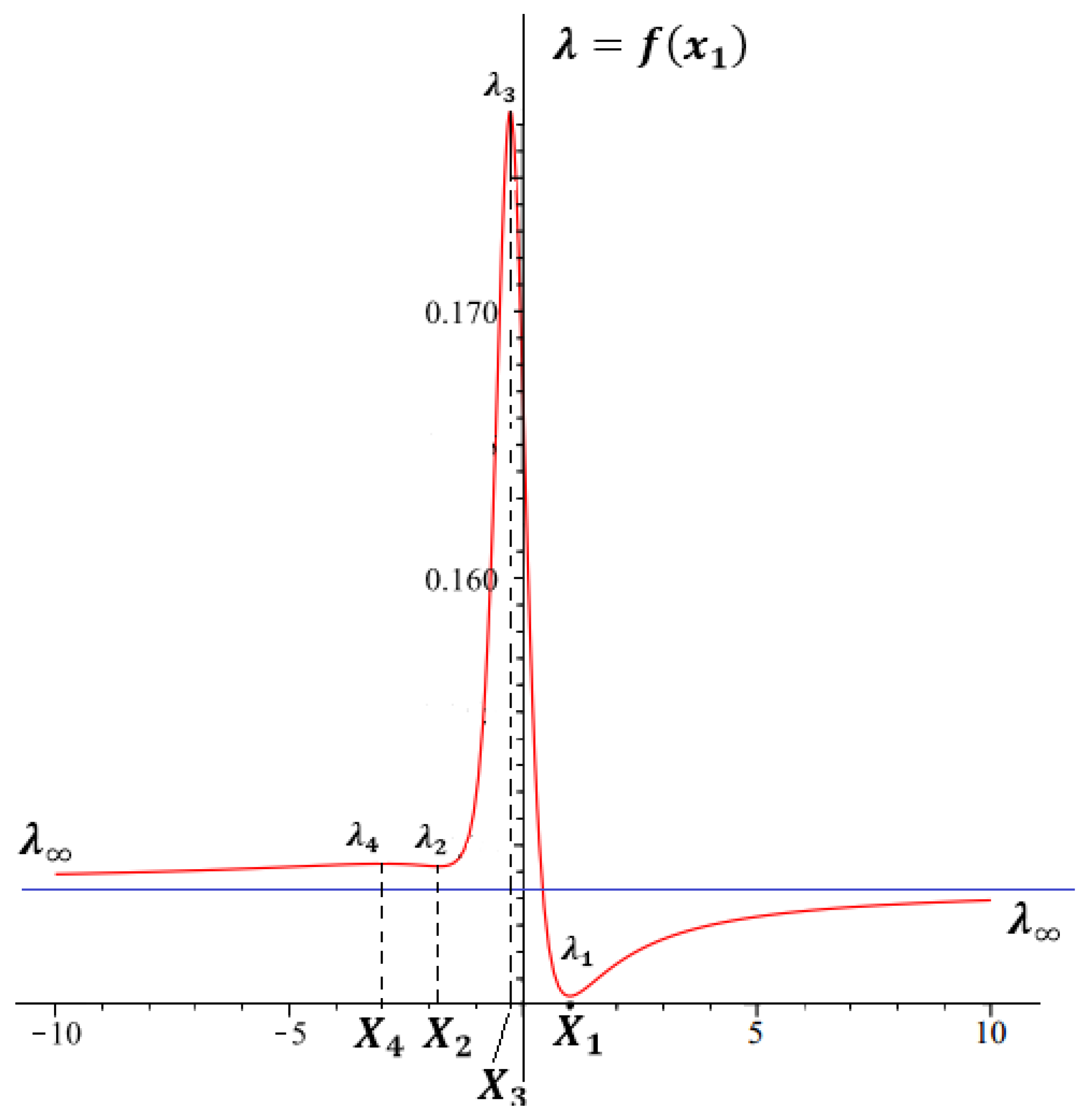
Proposition 2.

The solutions to Equations (4) and (5) for ansatz (7) imposed with $1<m$, $1<k_1=k_2=k$, $m\ne k$, obeying the inequalities $H\ne 0$, $H\ne h_1$, $H\ne h_2$, $h_1\ne h_2$, $S_1=mH+k{h}_1+k{h}_2\ne 0$ do exist if and only if $\alpha \epsilon >0$,

$${\lambda }_1<\lambda =\alpha \Lambda <{\lambda }_3$$

(113)

for $m<k$ and

$${\lambda }_3<\lambda =\alpha \Lambda <{\lambda }_1,$$

(114)

where ${\lambda }_1={\lambda }_1(k,k)$, ${\lambda }_3={\lambda }_3(k,k)$ are defined in (41) and (43). In this case H satisfies the relation (71) with X from (94), $x_1=h_1/H$ and $x_2=h_2/H$ are given by relations (88) and (89), λ obeys (101), (102) for ${ϵ}_1=-1$ and (109), (110) for ${ϵ}_1=1$ with ${\lambda }_{\infty }=\frac{k}{8(k-1)}$.

The case $H=0$. For $k_1=k_2=k>1$ and $H=0$ the solutions under consideration obeying restrictions (8) are absent [1].

5. The Analysis of Stability

Here, we analyse the stability of our solutions along a line as was done in Refs. [20,21,22].

We impose the following restriction:

$$det\left(L_{ij}\left(v\right)\right)\ne 0,$$

(115)

where

$$L=\left(L_{ij}\left(v\right)\right)=(2G_{ij}-4\alpha \epsilon G_{ijks}{v}^k{v}^s).$$

(116)

Here, one should deal with general cosmological type setup with the metric:

$$g=-\epsilon du\otimes du+\sum _{i=1}^n{e}^{2{\beta }^i\left(u\right)}{\epsilon }_{i}d{y}^i\otimes d{y}^i,$$

(117)

where $\epsilon =\pm 1$, ${\epsilon }_i=\pm 1$, $i=1,\dots ,n$. For the equations of motion we obtain [28]:

$$\begin{array}{c}\hfill E=G_{ij}{h}^i{h}^j+2\Lambda \epsilon -\alpha \epsilon G_{ijkl}{h}^i{h}^j{h}^k{h}^l=0,\end{array}$$

(118)

$$\begin{array}{c}\hfill Y_i=\frac{d{L}_i}{dt}+\left(\sum _{j=1}^n{h}^j\right)L_i-\frac{2}{3}(G_{sj}{h}^s{h}^j-4\Lambda \epsilon )=0,\end{array}$$

(119)

where $h^i={\dot{\beta }}^i=\frac{d{\beta }^i}{du}$,

$$L_i=L_i\left(h\right)=2G_{ij}{h}^j-\frac{4}{3}\alpha \epsilon G_{ijkl}{h}^j{h}^k{h}^l,$$

(120)

$i=1,\dots ,n$.

According to previous consideration of Ref. [21] the solution $\left(h^i\left(t\right)\right)=\left(v^i\right)$ ($i=1,\dots ,n$; $n>3$) to Equations (118) and (119) which obeys the restrictions (115) is stable under perturbations:

$$h^i\left(t\right)=v^i+\delta h^i\left(t\right),$$

(121)

$i=1,\dots ,n$, as $u\to +\infty$, if and only if

$$S_1\left(v\right)=\sum _{i=1}^n{v}^i>0$$

(122)

and it is unstable, as $u\to +\infty$, if and only if

$$S_1\left(v\right)=\sum _{i=1}^n{v}^i<0.$$

(123)

In the limit $u\to -\infty$, the stability condition is given by (123) while the instability condition reads as (122). These conditions just follow from solutions for perturbations $\delta h^i\left(t\right)=C_{i}exp(-S_1\left(v\right)u)$ ($C_i=\mathrm{const}\ne 0$) which are valid in the leading order.

Here, a key point is the verification of the relation (115). It was fulfilled in Ref. [22] by using first three relations in (8) and (14) and $k_1>1$, $k_2>1$ and $m>1$.

First we consider the case $1<m<k_1<k_2$. By using (18) we find that for $H>0$ the condition (122) may be written as:

$$m+k_1{x}_1+k_2{x}_2=1+x_1+x_2>0$$

(124)

or, equivalently,

$$x_1>X_4=\frac{m-k_2}{k_2-k_1}.$$

(125)

For $H<0$ the stability condition (122) is as follows:

$$x_1<X_4.$$

(126)

The non-stability condition (123) for $u\to +\infty$ reads as (126) for $H>0$ and as (125) for $H<0$. These conditions are reversed in case $u\to -\infty$.

Proposition 3.

Let us consider cosmological type solutions to Equations (4) and (5) for ansatz (7) with $1<k_1<k_2$, obeying the inequalities $H\ne 0$, $H\ne h_1$, $H\ne h_2$, $h_1\ne h_2$, $S_1=mH+k_1{h}_1+k_2{h}_2\ne 0$.

(a) 

Let $H>0$. For $u\to +\infty$ the solutions are stable if $x>X_4$ and unstable if $x<X_4$, while for $u\to -\infty$ they are stable if $x<X_4$ and unstable if $x>X_4$;

(b) 

Let $H<0$. For $u\to +\infty$ the solutions are stable if $x<X_4$ and unstable if $x>X_4$, while for $u\to -\infty$ they are stable if $x>X_4$ and unstable if $x<X_4$.

Now we proceed with considering the case $H\ne 0$, $1<m$, $1<k_1=k_2=k$, $m\ne k$. Since $x_1\ne 1$, $x_2\ne 1$ and $x_1\ne x_2$ the exact solutions under consideration obey the first three relations in (8), which imply the validity of the key restriction (115).

For the stability condition (122) as $u\to +\infty$ in this case we get:

$$H(m+k_1{x}_1+k_2{x}_2)=H(1+x_1+x_2)=H\left(1-\frac{m-1}{k-1}\right)>0,$$

(127)

or, equivalently,

$$H(k-m)>0.$$

(128)

The non-stability condition (123) for $u\to +\infty$ may be written as:

$$H(k-m)<0.$$

(129)

Thus, we have the following proposition.

Proposition 4.

Let us consider cosmological type solutions (4), (5) for ansatz (7) with $1<m$, $1<k_1=k_2=k$, $m\ne k$, obeying the inequalities $H\ne 0$, $H\ne h_1$, $H\ne h_2$, $h_1\ne h_2$, $S_1=mH+k{h}_1+k{h}_2\ne 0$, is stable, as $u\to +\infty$, if and only if $H(k-m)>0$ and it is unstable, as $u\to +\infty$, if and only if $H(k-m)<0$.

(c) 

Let $H>0$. For $u\to +\infty$ the solutions are stable if $k>m$ and unstable if $k<m$, while for $u\to -\infty$ they are stable if $k<m$ and unstable if $k>m$.

(d) 

Let $H<0$. For $u\to +\infty$ the solutions are stable if $k<m$ and unstable if $k>m$, while for $u\to -\infty$ they are stable if $k>m$ and unstable if $k<m$

The case $H=0$. For a completeness we consider the solutions with $H=0$ and $h_1$, $h_2$ from (64) and (65), where $k_1\ne k_2$, $k_1>1$, $k_2>1$, $\alpha \epsilon >0$ and $\Lambda$ is given by (63). We get:

$$S_1=k_1{h}_1+k_2{h}_2=\pm (k_2-k_1){\left(2\alpha \epsilon (k_1-1)(k_2-1)(k_1+k_2-2)\right)}^{-1/2}.$$

(130)

Here, ± is a sign parameter in (64) and (65). By using our analysis presented above we obtain that the solution with $\pm (k_2-k_1)>0$ is stable, as $u\to +\infty$. This occurs if either $k_2>k_1$ and the sign $‘‘+"$ are selected in (64) and (65), or if $k_2<k_1$ and the sign $‘‘-"$ are chosen. For the case $\pm (k_2-k_1)<0$ our solution is unstable, as $u\to +\infty$. (Here we also assume the restriction $m>1$). These conditions are reversed in case $u\to -\infty$.

6. Conclusions

We have studied the D-dimensional Einstein–Gauss–Bonnet (EGB) model with the $\Lambda$-term and two non-zero constants ${\alpha }_1$ and ${\alpha }_2$. By dealing with diagonal cosmological type metrics, we have considered a class of solutions with exponential dependence of three scale factors (upon u-variable) for any $\alpha ={\alpha }_2/{\alpha }_1\ne 0$, signature parameter $\epsilon =\pm 1$ and generic dimensionless parameter $\Lambda \alpha$.

More precisely speaking, we have described a class of cosmological type solutions with exponential dependence of three scale factors, governed by three non-coinciding Hubble-like parameters H, $h_1$ and $h_2$. These parameters correspond, respectively, to factor spaces of dimensions $m>1$, $k_1>1$ and $k_2>1$ ($D=1+m+k_1+k_2$), and obey the following restriction $S_1=mH+k_1{h}_1+k_2{h}_2\ne 0$. We have analyzed two cases: (i) $m<k_1<k_2$ and (ii) $1<k_1=k_2=k\ne m$. This choice does not restrict the generality, since, as it was shown, there are no solutions under consideration for $k_1=k_2=m$). It was shown that the solutions exist only if $\lambda =\alpha \Lambda >0$ and the (dimensionless) parameter $\lambda$ obey certain restrictions, e.g., upper and lower bounds for $H\ne 0$, which depend upon dimensions m, $k_1$ and $k_2$ (Proposition 1). In case (ii) we have presented explicit solutions for all $k>1$ and $k\ne m$ ( Proposition 2).

By using the Chirkov–Pavluchenko–Toporensky splitting trick from Ref. [17], we have reduced the problem for $H\ne 0$ to a master equation on the dimensionless variable $x_1=h_1/H$. This equation is of the fourth order (in the generic case) or less (depending on $\lambda$), and may be solved in radicals for all $m>1$, $k_1>1$, $k_2>1$ and $\lambda$. The master equation does not depend upon the signature parameter $\epsilon =\pm 1$ which only controls the sign of $\alpha$ according to inequality $\alpha \epsilon >0$. Due to bounds obtained $\lambda =\alpha \Lambda >0$. (This is valid also for $H=0$). Hence the solutions under consideration do exist if $\Lambda \epsilon >0$, i.e., when $\Lambda >0$ in the cosmological case ($\epsilon =1$) and $\Lambda <0$ in the static case ($\epsilon =-1$). Here there are no solutions under consideration for $\Lambda =0$—contrary to the case of two factor spaces [29,32].

Here we have analyzed the stability of solutions as $u\to \pm \infty$ in a class of cosmological type solutions with diagonal metrics. In both cases ((i) and (ii)) for $H\ne 0$, the “islands” of stability and instability were singled out. (The case $H=0$ was also analysed.) We have shown that in case (i) the solutions with $H>0$ are stable as $u\to \infty$ for $x_1=h_1/H>X_4=\frac{m-k_2}{k_2-k_1}$ and unstable as $u\to \infty$ for $x_1<X_4$ (see Proposition 3). These conditions should be reversed when we consider the case $H>0$, $u\to -\infty$ or we deal with $H<0$, $u\to +\infty$ (see Proposition 3). It was proved that in case (ii), the solutions with $H>0$ are stable as $u\to \infty$ for $k>m$ and unstable as $u\to \infty$ for $k<m$ (see Proposition 4). For a given choice of asymptotic $u\to \pm \infty$, the stability condition for $H<0$ is equivalent to the instability conditions for $H>0$ and vice versa.

We have also found that the solution with $H=0$ exists only for $k_1\ne k_2$, $\alpha \epsilon >0$ and a fixed value of $\epsilon \Lambda >0$ depending upon $k_1$ and $k_2$. Here we have two opposite in sign solutions for $(h_1,h_2)$ with one solution being stable ($u\to \pm \infty$) and the second one unstable, depending upon the sign of $k_1-k_2$.

Some cosmological applications of the model ($\epsilon =1$), e.g., in the context of the variation of the gravitational constant, were considered in Refs. [1,33,34]. For the static case ($\epsilon =-1$), possible applications of the obtained solutions may be a subject of a further research, aimed towards a search for topological black hole solutions (with flat horizon) or wormhole solutions, which are coinciding asymptotically (for ($u\to \pm \infty$)) with our solutions.