On the Error Estimation of the FEM for the Nikol’skij-Lizorkin Problem with Degeneracy in the Lebesgue Space

Abstract

In this manuscript, the Nikol’skii-Lizorkin problem with degeneracy on the entire boundary of the domain is considered. The degeneracy is caused by the behavior of the coefficients and right-hand sides of the problem on the boundary. The triangulation of the domain with a special compression to the boundary of the domain is carried out and the finite element method is constructed. An estimate for the rate of convergence of an approximate solution to an exact solution with the second order in the mesh step in the $L_2(\Omega )$ space norm is proved. Numerical experiments have confirmed the established estimate of the convergence rate.

1. Introduction

Boundary value problems for equations and systems of partial differential equations with a singularity play an important role in the mathematical modeling of processes in fracture mechanics (see, for example, [1,2]). The singularity can be caused by the presence of reentrant corners on the boundary of the two-dimensional domain or by the degeneracy of the coefficients and right-hand sides of the equation and boundary conditions. Classical methods of finite elements and difference schemes make it possible to find an approximate solution to these problems with low accuracy. The rate of convergence of the approximate solution to the exact one depends on the regularity of the solution of the differential problem [3].

It is known (see, for example, ([4,5,6,7]) that the solution of a two-dimensional boundary value problem in the presence of a corner singularity contains a singular component that depends on the distance $\rho$ to the vertex of the corner with an exponent $\mu$. The value of $\mu$ is determined by the size of the corner $\omega$ and $0.25<\mu <1$ for $\pi <\omega \le 2\pi$. In this case, the solution belongs to the space $W_2^{1+\mu -\epsilon }(\Omega )$, where $\mu =\pi /\omega$ for the Neumann or Dirichlet problem and $\mu =\pi /2\omega$ for the mixed boundary value problem, $\epsilon$ is an arbitrary positive number. The approximate solution found by classical numerical methods will converge to the exact solution at a rate of $O\left(h^{\mu }\right)(\mu <1)$ with respect to the mesh step h in the space $W_2^1(\Omega )$.

Numerical methods must consider the behavior of the solution in the neighborhood of the singularity point to increase the rate of convergence of the approximate solution to the value $O\left(h\right)$. A detailed list of such methods is given in [8,9]. We distinguish from these methods the extended finite element method (XFEM) [10,11,12,13] and the weighted finite element method (WFEM) [14,15,16,17]. The weighted finite-element method is based on the definition of the $R_{\nu }$-generalized solution [18,19,20] and the introduction of weighted basis functions [14,15,16,17] that consider the asymptotic behavior of the solution in the neighborhood of the singularity point. This allows one to find an approximate solution with a convergence rate $O\left(h\right)$ regardless of the size of the reentrant corner $\omega$.

Boundary value problems for elliptic equations with degeneracy on the entire boundary of the domain were considered by S.M. Nikol’sky and P.I. Lizorkin in the articles [21,22,23,24]. The degeneracy was caused by the behavior of the coefficients and right-hand sides of the problem on the boundary of the domain. The questions of the existence and uniqueness of the solution, and its coercive and differential properties were studied in the articles of these authors. For the numerical solution of the Dirichlet problem for an equation with degeneracy on the entire boundary of the domain, a finite element method was developed on the uniform mesh and mesh with compression to the boundary, which ensured the convergence of the approximate solution to the exact one [25]. In [9], an estimate for the rate of convergence $O\left(h\right)$ in the norm of the Sobolev weighted space was proved under a special compression of the mesh and conditions under which the solution of the differential problem belongs to the space ${\mathring{W}}_{2,\beta -1}^2(\Omega )$ (see [26]). In this paper, we prove an estimate for the rate of convergence $O\left(h^2\right)$ in the norm of the space $L_2(\Omega )$ and carry out the results of numerical experiments for two model problems.

We organize the remaining part of this paper as follows: Section 2 introduces the weighted Sobolev spaces and auxiliary statements. In Section 3 the Nikol’skij-Lizorkin boundary value problem and the auxiliary problem with degeneration on the entire boundary of the domain are presented. We have established the continuity and W-ellipticity of the bilinear form and formulated a theorem on the belonging of the solution of the problem in the space ${\mathring{W}}_{2,\beta -1}^2(\Omega )$. A scheme for the finite element method on a mesh with a special exponent of the degree of compression to the boundary is given in Section 4. In Section 5, an estimate for the rate of convergence of an approximate solution to an exact solution with the second-order mesh step in the norm of space $L_2(\Omega )$ is established. We present the results of numerical experiments for two model boundary value problems with degeneracy on the entire boundary for a symmetrical domain using our finite element method in Section 6.

2. Weighted Spaces

Throughout this paper, we assume that $\Omega \subset R^2=\left\{x=(x_1,x_2):x_i\in R,i=1,2\right\}$ is a bounded convex domain, its boundary $\partial \Omega$ is twice differentiable, and $\overline{\Omega }=\Omega \cup \partial \Omega$. By ${\Omega }_1$ we denote the boundary strip of width $b>0$.

We suppose that $\rho \left(x\right)>0$ is twice differentiable function for $x\in \Omega$ and coincides in ${\Omega }_1$ with the distance from x to the boundary $\partial \Omega$.

We denote by $W_{2,\gamma }^s(\Omega )$ the weighted Sobolev space of functions f with the norm

$${\parallel f\parallel }_{W_{2,\gamma }^s(\Omega )}={\parallel f\parallel }_{L_2(\Omega )}+{\left|f\right|}_{W_{2,\gamma }^s(\Omega )}.$$

(1)

Here

$$\begin{array}{c}{\parallel f\parallel }_{L_2(\Omega )}={\left({\int }_{\Omega }{f}^{2}dx\right)}^{\frac{1}{2}},\\ {\left|f\right|}_{W_{2,\gamma }^s(\Omega )}=\sum _{\begin{array}{c}{m}_1,m_2=0\\ \left|m\right|=s\end{array}}\parallel {\rho }^{-\gamma }\frac{{\partial }^{\left|m\right|}f}{\partial x_1^{m_1}\partial x_2^{m_2}}{\parallel }_{L_2(\Omega )},\end{array}$$

$m=(m_1,m_2)$, $m_i\ge 0$ are integers $(i=1,2)$, and $\left|m\right|=m_1+m_2$; $\gamma$ is a real number satisfying the inequalities $\frac{1}{2}-s<\gamma <\frac{1}{2}$; $s=1,2$; $dx=d{x}_{1}d{x}_2$.

We denote by ${\mathring{W}}_{2,\gamma }^s(\Omega )$ the subspace of the space $W_{2,\gamma }^s(\Omega )$ consisting of functions in $W_{2,\gamma }^s(\Omega )$ whose trace on $\partial \Omega$ is equal to zero.

We introduce the weighted Lebesgue space of functions f with the norm

$$\begin{array}{c}{\parallel f\parallel }_{L_{2,-\gamma }(\Omega )}={\left({\int }_{\Omega }{\left|{\rho }^{\gamma }f\right|}^{2}dx\right)}^{\frac{1}{2}}.\end{array}$$

We now formulate the following auxiliary statements (see [21,27]).

Lemma 1.

There is an embedding of spaces

$$W_{2,\gamma }^s(\Omega )\subset W_{2,{\gamma }_l}^{s-l}(\Omega )$$

for ${\gamma }_l<\frac{1}{2}$, ${\gamma }_l\le \gamma +l$, $0\le l\le s$.

Lemma 2.

If $f\in {\mathring{W}}_{2,\gamma }^s(\Omega )$, $s=1,2$, and $\frac{1}{2}-s<\gamma <\frac{1}{2}$, then

$${\parallel f\parallel }_{L_2(\Omega )}\le C_1{\left|f\right|}_{W_{2,\gamma }^s(\Omega )},$$

(2)

$${\parallel f\parallel }_{L_{2,s+\gamma }(\Omega )}\le C_2{\left|f\right|}_{W_{2,\gamma }^s(\Omega )},$$

(3)

where $C_1$, $C_2$ are positive constants independent of f.

3. Nikol’skij-Lizorkin Problem with Degeneracy

Let us consider the following problem

$${Lu=F,x\in \Omega ,u|}_{\partial \Omega }=0,$$

(4)

where

$$Lu\equiv -\sum _{k,l=1}^2\frac{\partial }{\partial x_k}\left(a_{kl}\left(x\right)\frac{\partial u}{\partial x_l}\right)+a\left(x\right)u,x\in \Omega .$$

We will suppose that the right-hand side F in (4) satisfies the condition

$$F\in L_{2,-1-\alpha }(\Omega ),$$

(5)

i.e., ${\rho }^{1+\alpha }F\in L_2(\Omega )$, the coefficients $a_{kl}\left(x\right)=a_{lk}\left(x\right)$, $(k,l=1,2)$ are differentiable functions in $\Omega$, satisfying the inequalities

$$|a_{kl}\left(x\right)|\le C_3{\rho }^{-2\alpha }\left(x\right),$$

(6)

$$\left|\frac{\partial a_{kl}\left(x\right)}{\partial x_1}\right|,\left|\frac{\partial a_{kl}\left(x\right)}{\partial x_2}\right|\le C_4{\rho }^{-2\alpha -1}\left(x\right),$$

(7)

and

$$\sum _{k,l=1}^2{a}_{kl}\left(x\right){\xi }_k{\xi }_l\ge C_5{\rho }^{-2\alpha }\left(x\right)\sum _{k=1}^2{\xi }_k^2,x\in \Omega ,C_5>0,$$

(8)

where ${\xi }_1,{\xi }_2$ are any real parameters, the function $a\left(x\right)$ is positive and satisfies the inequality

$$\left|a\left(x\right)\right|\le C_6{\rho }^{-2\alpha -2}\left(x\right),x\in \Omega .$$

(9)

Here $C_i$ ($i=3,\dots ,6$) are constants independent of x; $\alpha \in \left(-\frac{1}{2},\frac{1}{2}\right)$.

Introducing the bilinear form

$$E(u,v)={\int }_{\Omega }\left(\sum _{k,l=1}^2{a}_{kl}\frac{\partial u}{\partial x_k}\frac{\partial v}{\partial x_l}+auv\right)dx,$$

and the linear form

$$(F,v)={\int }_{\Omega }Fvdx,$$

we give a weak formulation to problem (4): find $u\in {\mathring{W}}_{2,\alpha }^1(\Omega )$ such that

$$E(u,v)=(F,v)\forall v\in {\mathring{W}}_{2,\alpha }^1(\Omega ).$$

(10)

A function u in ${\mathring{W}}_{2,\alpha }^1(\Omega )$ satisfying the equality (10) is called a generalized solution of the Dirichlet problem with degeneration.

We will need the following statement.

Lemma 3.

Suppose that conditions (5), (6), (8), (9) hold.

Then the bilinear form $E(u,v)$ is continuous and ${\mathring{W}}_{2,\alpha }^1(\Omega )$—elliptical, and the linear form $(F,v)$ is continuous on ${\mathring{W}}_{2,\alpha }^1(\Omega )$.

Proof. 

By means of conditions (5), (6), (9), the Cauchy-Schwarz inequality and the estimate (3) for $s=1,\gamma =\alpha$ (see Lemma 2) we establish the continuity of the bilinear and linear forms:

$$\left|E(u,v)\right|\le C_7{\parallel u\parallel }_{W_{2,\alpha }^1(\Omega )}{\parallel v\parallel }_{W_{2,\alpha }^1(\Omega )},u,v\in {\mathring{W}}_{2,\alpha }^1(\Omega ),$$

(11)

$$\left|(F,v)\right|\le C_8{\parallel F\parallel }_{L_{2,-1-\alpha }(\Omega )}{\parallel v\parallel }_{W_{2,\alpha }^1(\Omega )},v\in {\mathring{W}}_{2,\alpha }^1(\Omega ).$$

Using the condition (8) and inequality (2) for $s=1,\gamma =\alpha$ we prove the ${\mathring{W}}_{2,\alpha }^1(\Omega )$—ellipticity of the bilinear form:

$$\begin{array}{c}E(u,u)\ge C_9{\parallel u\parallel }_{W_{2,\alpha }^1(\Omega )}^2,u\in {\mathring{W}}_{2,\alpha }^1(\Omega ).\end{array}$$

□

The existence and uniqueness of a generalized solution of the problem (4) in the space ${\mathring{W}}_{2,\alpha }^1(\Omega )$ follow from Lemma 3 and Lax-Milgram’s theorem (see [3]).

If conditions (5)–(9) are satisfied then the generalized solution of the Dirichlet problem (4) belongs to the space ${\mathring{W}}_{2,\alpha -1}^2(\Omega )$ (see [23]) and the operator $L:{\mathring{W}}_{2,\alpha -1}^2(\Omega )\to L_{2,-1-\alpha }$ has a bounded inverse operator (see [24]).

Following [26], we introduce an auxiliary problem

$$\begin{array}{c}\tilde{L}{v=\Phi ,v|}_{\partial \Omega }=0,\end{array}$$

where

$$\begin{array}{c}\tilde{L}v\equiv Lv+\lambda L_{1}v,\Phi ={\rho }^{-\lambda }F,\alpha <\alpha +\lambda <\frac{1}{2},\\ Lv=-\sum _{k,l=1}^2\frac{\partial }{\partial x_k}\left(a_{kl}\frac{\partial v}{\partial x_l}\right)+av,\\ L_{1}v=-\sum _{k,l=1}^2(\frac{\partial a_{kl}}{\partial x_k}\frac{\partial \rho }{\partial x_l}\frac{v}{\rho }+a_{kl}(\lambda -1)\frac{\partial \rho }{\partial x_l}\frac{\partial \rho }{\partial x_k}\frac{v}{{\rho }^2}+\\ +a_{kl}\frac{{\partial }^2\rho }{\partial x_k\partial x_l}\frac{v}{\rho }+\frac{a_{kl}}{\rho }\frac{\partial \rho }{\partial x_l}\frac{\partial v}{\partial x_k}+\frac{a_{kl}}{\rho }\frac{\partial \rho }{\partial x_k}\frac{\partial v}{\partial x_l}).\end{array}$$

Now we formulate the main result of the paper [26] for $\lambda =\beta -\alpha$.

Theorem 1.

If the coefficients $a_{kl}=a_{lk}(k=1,2)$ of Equation (4) satisfy inequalities (6)–(9) for some $\alpha \in (-\frac{1}{2},\frac{1}{2})$ and conditions

$$\begin{array}{c}F\in L_{2,-1-2\alpha +\beta }(\Omega )\end{array}$$

and

$$(\beta -\alpha )\parallel L_1{\parallel }_{{\mathring{W}}_{2,\alpha -1}^2\to L_{2,-1-\alpha }}{\parallel L^{-1}\parallel }_{L_{2,-1-\alpha }\to {\mathring{W}}_{2,\alpha -1}^2}<1,\alpha <\beta <\frac{1}{2}$$

(12)

are satisfied, then the generalized solution u belongs to the space ${\mathring{W}}_{2,\alpha -1}^2(\Omega )$ and, moreover,

$${\parallel u\parallel }_{W_{2,\beta -1}^2(\Omega )}\le C_{10}{\parallel F\parallel }_{L_{2,-1-2\alpha +\beta }(\Omega )}.$$

(13)

4. Finite Element Method

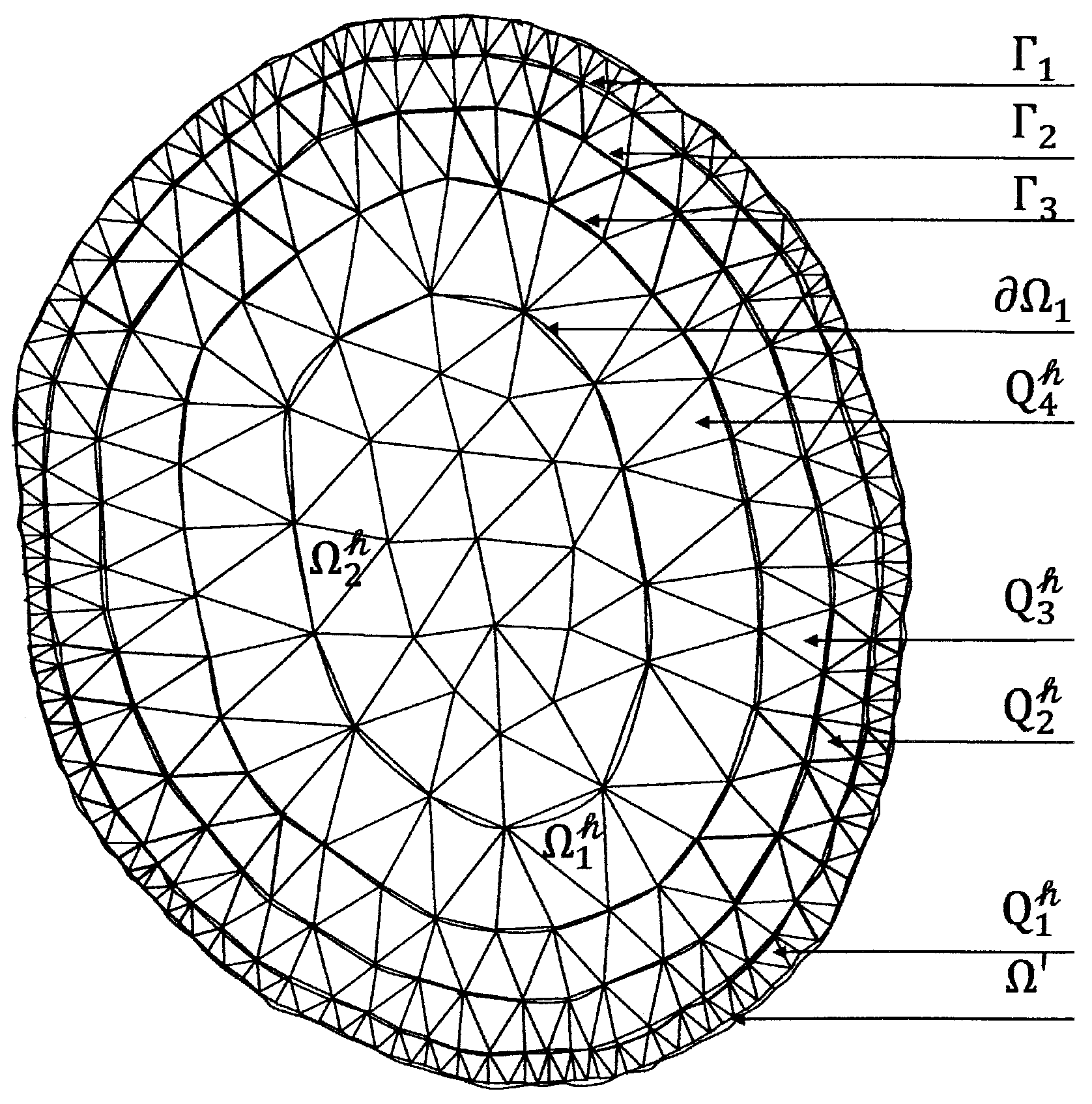
The finite element method for finding an approximate generalized solution to the Dirichlet problem (10) was constructed in [9]. Here we briefly describe the construction of the scheme FEM the first step of which is triangulation $T_h$ of the domain $\Omega$ (see, for example, Figure 1).

Figure 1. The triangulation $T_h$ of the domain $\Omega$ [9].

Assuming that ${\delta }_{\Omega }$ is the diameter of the circle inscribed in $\Omega$, and the width b of boundary strip ${\Omega }_1$ satisfies the inequality $b<\frac{{\delta }_{\Omega }}{2}$, we draw the curves ${\Gamma }_j$ at distance $b{\left(\frac{j}{n}\right)}^r$, $j=0,\dots ,n$, to the boundary $\partial \Omega$. (Here ${\Gamma }_0=\partial \Omega ,r$ denotes the exponent of compression and $r>1$). In this case, the domain $\Omega$ is divided by the line ${\Gamma }_n$ into two subdomains ${\Omega }_1$ and ${\Omega }_2=\Omega \backslash {\Omega }_1$. (Here ${\Gamma }_n=\partial {\Omega }_1$).

Let $l_j,j=0,\dots ,n$, denotes the length of the curve ${\Gamma }_j$. We fix $M_j,j=0,\dots ,n$, equidistant points on each curve ${\Gamma }_j$ and call them grid nodes. Number $M_j=\left[l_j/\left(b\left({\left(\frac{j}{n}\right)}^r-{\left(\frac{j-1}{n}\right)}^r\right)\right)\right]+1,j=1,\dots ,n,M_0=2M_1$. (Here $\left[x\right]$ denotes the integer part of x).

First, the nodes of the curve ${\Gamma }_j(j=0,\dots ,n)$ are connected by the broken line. Then, we connect each node on the curve ${\Gamma }_{j-1}$, $j=1,\dots ,n$, with the nearest nodes on the curve ${\Gamma }_j$. Thus, we triangulated the boundary strip ${\Omega }_1$ with compression of the triangles to the boundary $\partial \Omega$. We will call the set of the triangles with vertices on ${\Gamma }_{j-1}$ and ${\Gamma }_j$ a layer and denote it by $Q_j^h$. (Here h is the maximal length of the sides of the triangles in $Q_n^h$). For instance, in Figure 1 the subdomain ${\Omega }_1$ has the layers $Q_1^h,\dots ,Q_4^h$, ${\Gamma }_4=\partial {\Omega }_1$ and ${\Omega }_1^h={\bigcup }_{j=1}^4{Q}_j^h$.

We now perform a quasi-uniform triangulation of the subdomain ${\Omega }_2$. Note that the sides of triangles from ${\Omega }_2$ can not be greater than h and the vertices coincide on the boundary $\partial {\Omega }_1$ for triangles from ${\Omega }_1$ and ${\Omega }_2$.

As a result, we have the triangulation $T_h$ of the domain $\Omega$ so that:

(a)

${\displaystyle {\Omega }^h=\bigcup _{i=1}^N{K}_i}$, $\left\{K\right\}=\{K_1,\dots ,K_N\}$, where $K_i$ is a closed triangle and is called a finite element. Let ${\Omega }_2^h={\Omega }^h\backslash {\Omega }_1^h$.

(b)

${\Omega }^{{}^{\prime }}=\overline{\Omega }\backslash {\Omega }^h$ is the set of segments cut off from $\Omega$ by triangles K with vertices on the boundary $\partial \Omega$.

(c)

The intersection of any triangles $K_m,K_l\in K(m\ne l)$ is one common vertex or one whole side or is empty.

(d)

The smallest of the corners of the triangles K is always strictly positive.

We observe that the vertices $P_i,i=1,\dots ,N_h$ of the triangles are the nodes of the triangulation.

We now define the finite element space $V^h$ by

$$V^h=\left\{\begin{array}{cc}\hfill & v\mathrm{is}\mathrm{linear}\mathrm{on}\mathrm{each}{K}_i\in K,\hfill \\ v:\hfill & v\mathrm{vanishes}\mathrm{on}\overline{\Omega }\backslash {\Omega }^h\hfill \\ \hfill & \mathrm{and}v\mathrm{is}\mathrm{continious}\mathrm{in}\Omega ,\hfill \end{array}\right.$$

we concider the following discrete problem: find $u_h\in V^h$ such that

$$\mathrm{E}(u_h,v_h)=(\mathrm{F},v_h)\forall v_h\in V^h.$$

(14)

A function $u_h$ in $V^h$ satisfying the equality (14) is called an approximate (finite element) generalized solution of the Dirichlet problem with degeneration.

If will be found in the form

$$u_h\left(x\right)=\left\{\begin{array}{cc}{\displaystyle \sum _{i=1}^{N^{\prime }}}{a}_i{\psi }_i\left(x\right)\hfill & \mathrm{if}x\in {\Omega }^h,\hfill \\ 0\hfill & \mathrm{if}x\in \overline{\Omega }\backslash {\Omega }^h.\hfill \end{array}\right.$$

Here $N^{\prime }$ denotes the number of the internal nodes; ${\psi }_i\left(x\right)$ is a linear function over every triangle K, equals to 1 at the point $P_i$ and zero at all other nodes, $a_i=u_h\left(P_i\right)$.

Obviously that $V^h$ is a subset of ${\mathring{W}}_{2,\alpha }^1(\Omega )$. The existence and uniqueness of the approximate solution $u_h$ of the problem (14) follow by the Lax-Milgram theorem from properties of $E(u,v)$ and $(F,v)$ (see Lemma 3).

The following result states the estimate for the convergence of the finite element method.

Theorem 2

([9]).Let the coefficients of Equation (4) satisfy inequalities (6)–(9) for some $\alpha \in (-\frac{1}{2};\frac{1}{2})$ and conditions $F\in L_2,-1-2\alpha +\beta (\Omega )(\alpha <\beta <\frac{1}{2})$ and (12) are met.

Then there exists a constant $C_{11}$ independent of $u,u_h,F,h$ and such that for the triangulation $T_h$ of the domain Ω with exponent of compression $r=\frac{1}{\beta -\alpha }$ we have the convergence estimate

$$\parallel u-u_h{\parallel }_{W_{2,\alpha }^1(\Omega )}\le C_{11}h{\parallel F\parallel }_{L_2,-1-2\alpha +\beta (\Omega )}.$$

(15)

5. Error Estimate

We will obtain an apriori estimate of the convergence rate in the $L_2(\Omega )$ norm.

Taking into account the definition of the norm (1) in the space $W_{2,\alpha }^1(\Omega )$, we get from the estimate (15)

$$\parallel u-u_h{\parallel }_{L_2(\Omega )}\le C_{12}h{\parallel F\parallel }_{L_2,-1-2\alpha +\beta (\Omega )},$$

where $C_{12}>0$.

Let us show that we actually have

$$\parallel u-u_h{\parallel }_{L_2(\Omega )}=O\left(h^2\right).$$

We will use the Aubin-Nitsche idea for nonweighted spaces (see [28,29]). To do that, introduce the auxiliary problem:

$$Lw=G_h,x\in \Omega ,w{\mid }_{\partial \Omega }=0,$$

(16)

where

$$Lw=-\sum _{k,l=1}^2\frac{\partial }{\partial x_k}\left(a_{kl}\left(x\right)\frac{\partial w}{\partial x_l}\right)+a\left(x\right)w,x\in \Omega ,G_h=u-u_h.$$

Since the difference ($u-u_h$) is the element of the space $L_2(\Omega )$ and for $0<\beta -\alpha \le \frac{1}{2}$ the inequality $1+2\alpha -\beta >0$ is valid, then $G_h{\rho }^{1+2\alpha -\beta }$ belongs to the space $L_2(\Omega )$, i.e.,

$$G_h\in L_{2,-1-2\alpha +\beta }(\Omega ),\alpha <\beta <\frac{1}{2}.$$

(17)

We define a bilinear form

$$E(w,v)={\int }_{\Omega }\left(\sum _{k,l=1}^2{a}_{kl}\frac{\partial w}{\partial x_k}\frac{\partial v}{\partial x_l}+awv\right)dx$$

and linear form

$$\left(G_h,v\right)={\int }_{\Omega }{G}_{h}vdx$$

for the problem (16).

As well as (4), the problem (16) is equivalent to the following variational problem: find $w\in {\mathring{W}}_{2,\alpha }^1(\Omega )$, such that

$$E(w,v)=(G_h,v)\forall v\in {\mathring{W}}_{2,\alpha }^1(\Omega ).$$

(18)

A function w from the space ${\mathring{W}}_{2,\alpha }^1(\Omega )$ is called generalized solution to the problem (16) if it satisfies the equality (18).

Since the bilinear form $E(w,v)$ is continuous and ${\mathring{W}}_{2,\alpha }^1(\Omega )$—elliptical, and the linear form ($G_h,v$) is continuous on ${\mathring{W}}_{2,\alpha }^1(\Omega )$, the existence and uniqueness of a generalized solution of the problem (16) follow from Lax-Milgram theorem (see [3]).

Let us note that if $G_h\in L_{2,-1-2\alpha +\beta }(\Omega ),\alpha <\beta <\frac{1}{2}$, (i.e. ${\rho }^{1+2\alpha -\beta }{G}_h\in L_2(\Omega )$) and the condition (12) holds, then according to Theorem 1, w belongs to the space ${\mathring{W}}_{2,\beta -1}^2(\Omega )$ and the estimate

$${\parallel w\parallel }_{W_{2,\beta -1}^2(\Omega )}\le C_{13}{\parallel {\rho }^{1+2\alpha -\beta }{G}_h\parallel }_{L_2(\Omega )}$$

(19)

is valid.

A function $w_h$ in the space $V^h\subset {\mathring{W}}_{2,\alpha }^1(\Omega )$ satisfying the equality

$$E(w_h,v_h)=(G_h,v_h)\forall v_h\in V^h$$

is called an approximate (finite element) generalized solution to the auxiliary problem (16).

Similar to $u_h$, the function $w_h$ exists and is unique.

Taking into account (19), Theorem 2 implies the statement.

Lemma 4.

Let the coefficients of the Equation (16) satisfy inequalities (6)–(9) for some $\alpha \in \left(-\frac{1}{2};\frac{1}{2}\right),{\rho }^{1+2\alpha -\beta }{G}_h\in L_2(\Omega )$ and condition (12) is met.

Then there exists a constant $C_{14}$ not depending on $w,w_h,G_h$ and h such that the convergence estimate

$$\parallel w-w_h{\parallel }_{W_{2,\alpha }^1(\Omega )}\le C_{14}h{\parallel {\rho }^{1+2\alpha -\beta }{G}_h\parallel }_{L_2(\Omega )}$$

(20)

holds for the triangulation $T_h$ of the domain Ω with an exponent of compression $r=\frac{1}{\beta -\alpha }$.

Now we will establish the estimate of the convergence rate in the norm of the space $L_2(\Omega )$.

Theorem 3.

Let the conditions of Theorem 2 be satisfied. Then there exists a positive constant $C_{15}$ independent of $u,u_h,F$ and h such that the following convergence estimate holds:

$$\parallel u-u_h{\parallel }_{L_2(\Omega )}\le C_{15}{h}^2{\parallel F\parallel }_{L_{2,-1-2\alpha +\beta }(\Omega )}.$$

(21)

Proof. 

Taking into account that ($u-u_h$) belongs to the space ${\mathring{W}}_{2,\alpha }^1(\Omega )$ we have from the equality (18)

$$E(w,u-u_h)=(G_h,u-u_h).$$

Concidering that $G_h=u-u_h$ and using the equality

$$E(u-u_h,v_h)=0\forall v_h\in V^h,$$

with $v_h=w_h$, we get

$$(u-u_h,u-u_h)=E(w,u-u_h)-E(w_h,u-u_h)=E(w-w_h,u-u_h).$$

Due to the continuity on ${\mathring{W}}_{2,\alpha }^1(\Omega )$ of the bilinear form we have

$$\parallel u-u_h{\parallel }_{L_2(\Omega )}^2\le C_{16}\parallel u-u_h{\parallel }_{W_{2,\alpha }^1(\Omega )}{\parallel w-w_h\parallel }_{W_{2,\alpha }^1(\Omega )}.$$

Using the estimates (15) and (20), we obtain

$$\parallel u-u_h{\parallel }_{L_2(\Omega )}^2\le C_{17}{h}^2{\parallel F\parallel }_{L_{2,-1-2\alpha +\beta }(\Omega )}{\parallel {\rho }^{1+2\alpha -\beta }{G}_h\parallel }_{L_2(\Omega )}\le$$

$$\le C_{17}{h}^2\left(\underset{x\in \Omega }{max}{\rho }^{1+2\alpha -\beta }\left(x\right)\right){\parallel F\parallel }_{L_2,-1-2\alpha +\beta (\Omega )}{\parallel G_h\parallel }_{L_2(\Omega )}.$$

Since ${\parallel G_h\parallel }_{L_2(\Omega )}={\parallel u-u_h\parallel }_{L_2(\Omega )}$ then from the last inequality we establish the estimate (21). □

6. Numerical Experiments

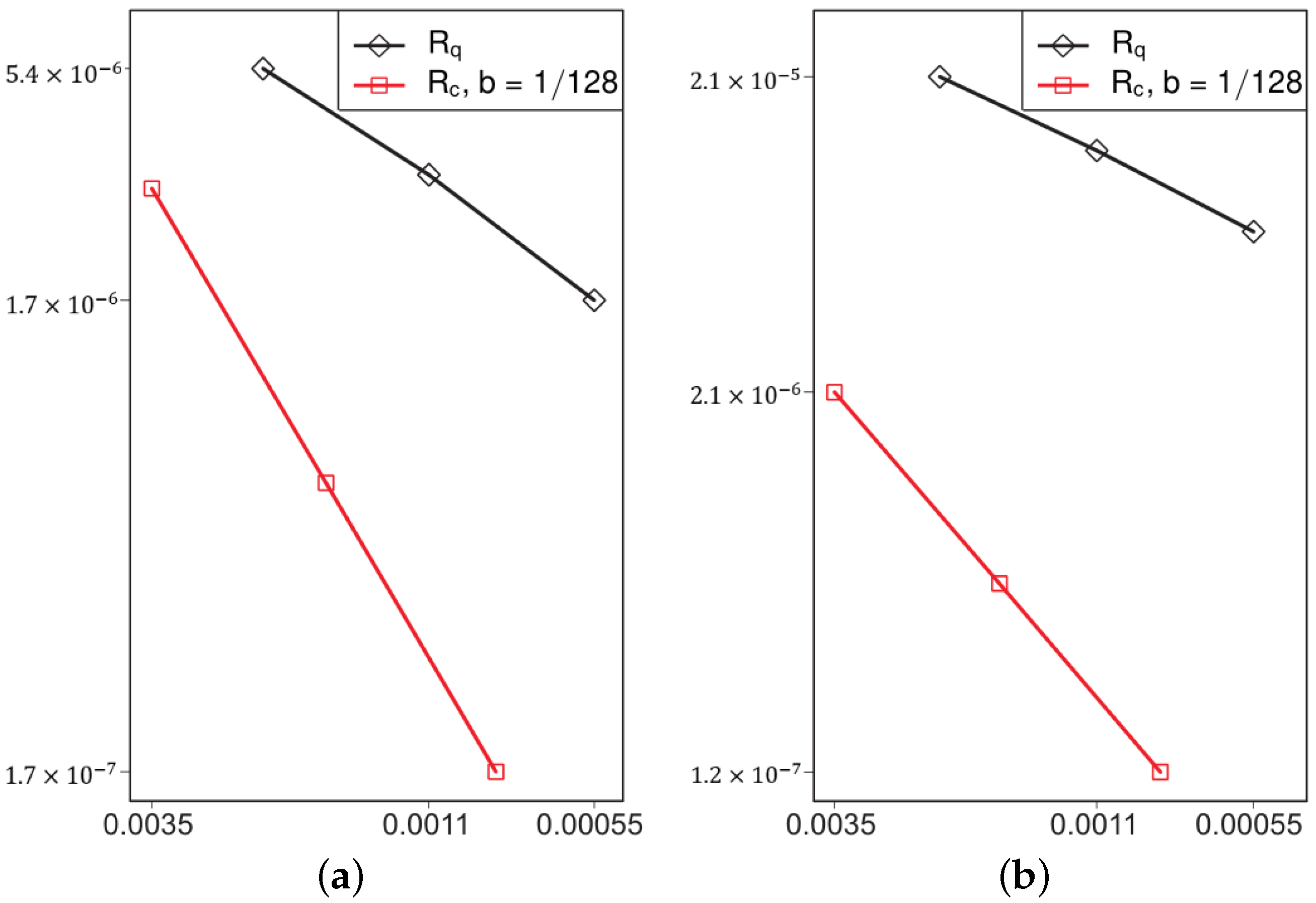
In this section, we demonstrate the validity of the convergence rate estimate (21) by the examples of test calculations of model problems. We compare the errors in the Lebesgue space norm for approximate solutions calculated by the finite element method on a quasi-uniform mesh ($R_q$) and a mesh with compression ($R_c$).

Let $\Omega$ be a circle of unit radius and with center at the point ($2;2$) (Figure 2), while the coefficients and the right side of Equation (4) are given as follows:

$$a_{11}\left(x\right)=a_{22}\left(x\right)={\rho }^{-2\alpha }\left(x\right),a\left(x\right)=1,$$

$$F\left(x\right)=-4(1+\beta -l)\left((\beta -2\alpha -l){\rho }^{\beta -2\alpha -l-1}\left(x\right)(1-\rho \left(x\right))-{\rho }^{\beta -2\alpha -l}\left(x\right)\right)+$$

$$+{\rho }^{1+\beta -l}\left(x\right),$$

where $\rho \left(x\right)=1-{(x_1-2)}^2-{(x_2-2)}^2,\alpha \in \left(-\frac{1}{2};\frac{1}{2}\right),\beta \in \left(\alpha ;\frac{1}{2}\right),l<\frac{1}{2}$.

Figure 2. The triangulation $T_h$ of the domain $\Omega$ for model problems.

The exact solution of this problem is $u\left(x\right)={\rho }^{1+\beta -l}\left(x\right)$.

The calculations were performed using the finite element method (see Section 3) and code [30].

Model problem 1. Let us set the parameters $\alpha =0.01, \beta =0.49, l=0.499,$ at which the coefficient and the right side of Equation (4) have the form

$$a_{11}\left(x\right)=a_{22}\left(x\right)={\rho }^{-0.02}\left(x\right),a\left(x\right)=1,$$

$$F\left(x\right)=0.114956·{\rho }^{-1.029}\left(x\right)+3.849044·{\rho }^{-0.029}\left(x\right)+{\rho }^{0.991}\left(x\right).$$

With such initial data, the exact solution of the problem is the function $u\left(x\right)={\rho }^{0.991}\left(x\right)$. The exponent of compression of the mesh is $r=2.08\left(3\right)$.

In Table 1 we present the difference between an exact and an approximate solutions in the norm of the space $L_2(\Omega )$, i.e., ${\parallel \psi \parallel }_{L_2(\Omega )}={\parallel u-u_h\parallel }_{L_2(\Omega )}$, for meshes $R_q$ and $R_c$. The parameter $\eta$ is the relation norms ${\parallel \psi \parallel }_{L_2(\Omega )}$ when the mesh parameter h is reduced two time. The parameter h decreases due to increase of the number n of the curves ${\Gamma }_j$ at a fixed value of the boundary strip $b=1/128$ for mesh $R_c$.

Table 1. The error ${\parallel \psi \parallel }_{L_2(\Omega )}$ for meshes $R_q$ and $R_c$ for Model problem 1.

Quasi-Uniform Mesh (${\mathit{R}}_{\mathit{q}}$)			Refined Mesh (${\mathit{R}}_{\mathit{c}}$), $\mathit{b}=1/128$
h	${\mathbf{\parallel }\mathbf{\psi }\mathbf{\parallel }}_{{\mathit{L}}_{\mathbf{2}}\mathbf{(}\mathbf{\Omega }\mathbf{)}}$	$\mathbf{\eta }$	$\mathit{n}$	$\mathit{h}$ in domain ${\Omega }_{\mathbf{2}}$	${\mathbf{\parallel }\mathbf{\psi }\mathbf{\parallel }}_{{\mathit{L}}_{\mathbf{2}}\mathbf{(}\mathbf{\Omega }\mathbf{)}}$	$\mathbf{\eta }$
0.0022	5.61 × 10${}^{-6}$		3	0.0035	$3.01\times {10}^{-6}$
		1.68				4.21
0.0011	$3.22\times {10}^{-6}$		8	0.00169	$7.12\times {10}^{-7}$
		1.83				4.11
0.00055	$1.74\times {10}^{-6}$		18	0.00083	$1.73\times {10}^{-7}$

Figure 3a shows change ${\parallel \psi \parallel }_{L_2(\Omega )}$ for meshes $R_q$ and $R_c$ depending on the change in parameter h.

Figure 3. Error ${\parallel \psi \parallel }_{L_2(\Omega )}$ dependence on the parameter h for meshes $R_q$ and $R_c$ for model problem 1 (a) and model problem 2 (b).

Model problem 2. Parameters $\alpha ,\beta ,l$ are chosen as follows: $\alpha =-0.49, \beta =0.01,$ $l=0.49.$ Then

$$a_{11}\left(x\right)=a_{22}\left(x\right)={\rho }^{0.98}\left(x\right),a\left(x\right)=1,$$

$$F\left(x\right)=-1.04·{\rho }^{-0.5}\left(x\right)+3.12·{\rho }^{0.5}\left(x\right)+{\rho }^{0.52}\left(x\right).$$

The exact solution of the problem is the function $u\left(x\right)={\rho }^{0.52}\left(x\right)$, the exponent of compression of the mesh is $r=2$. The results of the research of Model problem 2 are presented in Table 2 and Figure 3b.

Table 2. The error ${\parallel \psi \parallel }_{L_2(\Omega )}$ for meshes $R_q$ and $R_c$ for Model problem 2.

Quasi-Uniform Mesh (${\mathit{R}}_{\mathit{q}}$)			Refined Mesh (${\mathit{R}}_{\mathit{c}}$), $\mathit{b}=1/128$
h	${\mathbf{\parallel }\mathbf{\psi }\mathbf{\parallel }}_{{\mathit{L}}_{\mathbf{2}}\mathbf{(}\mathbf{\Omega }\mathbf{)}}$	$\mathbf{\eta }$	$\mathit{n}$	$\mathit{h}$ in domain ${\Omega }_{\mathbf{2}}$	${\mathbf{\parallel }\mathbf{\psi }\mathbf{\parallel }}_{{\mathit{L}}_{\mathbf{2}}\mathbf{(}\mathbf{\Omega }\mathbf{)}}$	$\mathbf{\eta }$
0.0022	$2.14\times {10}^{-5}$		3	0.0035	$2.07\times {10}^{-6}$
		1.72				4.14
0.0011	$1.24\times {10}^{-5}$		8	0.00169	$5.01\times {10}^{-7}$
		1.82				4.03
0.00055	$0.68\times {10}^{-5}$		18	0.00083	$1.24\times {10}^{-7}$

7. Conclusions

In this paper, we construct a finite element method for solving the Dirichlet problem for a second-order elliptic equation with degeneration on the entire twice continuously differentiable boundary of a two-dimensional domain $\Omega$. We have proved that the approximate solution of the problem (4) converges to the exact one with the rate $O\left(h^2\right)$ in the $L_2(\Omega )$ norm on meshes with the corresponding compression of nodes to the boundary. The convergence rate estimate from Theorem 3 was confirmed by test calculations for symmetrical domains.

The developed and studied finite element method schemes with mesh compression to the boundary of the domain can be used to solve problems of hydrodynamics, electromagnetism, diffusion, theory of plasticity, etc., leading to boundary value problems for elliptic equations with degeneracy on the boundary.

In the future, we plan to define an $R_{\nu }$-generalized solution (see [31,32,33]) for the Nikol’skii-Lizorkin problem. This will make it possible to achieve the convergence rate of the solution by the finite element method equal to $O\left(h^2\right)$ without compression of the mesh to the boundary. The dimension of the main matrix of the FEM system of equations will be significantly reduced and will be better structured. This will make it possible to find an approximate solution with a given accuracy faster and more economically.

References

1. Gdoutos, E.E. Engineering Applications of Fracture Mechanics. In Fracture Mechanics Criteria and Applications; Kluwer Academic Publishers: Dordrecht, The Netherlands, 1990; Volume 10. [Google Scholar]
2. Szabó, B.; Babuška, I. Finite Element Analysis; John Wiley & Sons: New York, NY, USA, 1991. [Google Scholar]
3. Ciarlet, P. The Finite Element Method for Elliptic Problems; Studies in Mathematics and Its Applications; North-Holland: Amsterdam, The Netherlands, 1978. [Google Scholar]
4. Kondrat’ev, V.A. Boundary-value problems for elliptic equations in domains with conical or angular points. Trans. Mosc. Math. Soc. 1967, 16, 227–313. [Google Scholar]
5. Mazya, V.G.; Plamenevskij, B.A. Lp-estimates of solutions of elliptic boundary value problems in domains with edges. Trans. Mosc. Math. Soc. 1980, 1, 49–97. [Google Scholar]
6. Grisvard, P. Boundary Value Problems in Non-Smooth Domains; Pitman: London, UK, 1985. [Google Scholar]
7. Dauge, M. Elliptic Boundary Value Problems on Corner Domains; Lecture Notes in Mathematics; Springer: Berlin, Germany, 1988; Volume 1341. [Google Scholar]
8. Rukavishnikov, V.A. Body of Optimal Parameters in the Weighted Finite Element Method for the Crack Problem. J. Appl. Comput. Mech. 2021, 7, 2159–2170. [Google Scholar] [CrossRef]
9. Rukavishnikov, V.A.; Rukavishnikova, E.I. Error estimate FEM for the Nikol’skij-Lizorkin problem with degeneracy. J. Comput. Appl. Math. 2022, 403, 113841. [Google Scholar] [CrossRef]
10. Moës, N.; Dolbow, J.; Belytschko, T. A finite element method for crack growth without remeshing. Int. J. Numer. Methods Eng. 1999, 46, 131–150. [Google Scholar] [CrossRef]
11. Nicaise, S.; Renard, Y.; Chahine, E. Optimal convergence analysis for the extended finite element method. Int. J. Numer. Methods Eng. 2011, 86, 528–548. [Google Scholar] [CrossRef] [Green Version]
12. Sukumar, N.; Dolbow, J.E.; Moës, N. Extended finite element method in computational fracture mechanics: A retrospective examination. Int. J. Fract. 2015, 196, 189–206. [Google Scholar] [CrossRef]
13. Zhou, X.; Chen, J.; Berto, F. XFEM based node scheme for the frictional contact crack problem. Comput. & Struct. 2020, 231, 106221. [Google Scholar] [CrossRef]
14. Rukavishnikov, V.A.; Nikolaev, S.G. On the Rν-generalized solution of the Lamé system with corner singularity. Dokl. Math. 2015, 92, 421–423. [Google Scholar] [CrossRef]
15. Rukavishnikov, V.A. Weighted FEM for Two-Dimensional Elasticity Problem with Corner Singularity. Lect. Notes Comput. Sci. Eng. 2016, 112, 411–419. [Google Scholar] [CrossRef]
16. Rukavishnikov, V.A.; Rukavishnikov, A.V. Weighted finite element method for the Stokes problem with corner singularity. J. Comput. Appl. Math. 2018, 341, 144–156. [Google Scholar] [CrossRef]
17. Rukavishnikov, V.A.; Mosolapov, A.O.; Rukavishnikova, E.I. Weighted finite element method for elasticity problem with a crack. Comput. Struct. 2021, 243, 106400. [Google Scholar] [CrossRef]
18. Rukavishnikov, V.A. On the uniqueness of the Rν-generalized solution of boundary value problems with noncoordinated degeneration of the initial data. Dokl. Math. 2001, 63, 68–70. [Google Scholar]
19. Rukavishnikov, V.A.; Kuznetsova, E.V. The Rν-generalized solution of a boundary value problem with a singularity belongs to the space W 2 , ν + β / 2 + k + 1 k + 2 ( Ω , δ ) . Differ. Equ. 2009, 45, 913–917. [Google Scholar] [CrossRef]
20. Rukavishnikov, V.A.; Rukavishnikova, E.I. Existence and uniqueness of an Rν-generalized solution of the Dirichlet problem for the Lamé system with a corner singularity. Differ. Equations 2019, 55, 832–840. [Google Scholar] [CrossRef]
21. Nikol’skij, S.M. A Variational Problem for an Equation of Elliptic Type with Degeneration on the Boundary. Proc. Steklov Inst. Math. 1981, 150, 227–254. [Google Scholar]
22. Lizorkin, P.I.; Nikol’skij, S.M. An elliptic equations with degeneracy. A variational method. Sov. Math. Dokl. 1981, 23, 237–240. [Google Scholar]
23. Lizorkin, P.I.; Nikol’skij, S.M. Elliptic equations with degeneracy. Differential properties of solutions. Sov. Math. Dokl. 1981, 23, 268–271. [Google Scholar]
24. Lizorkin, P.I.; Nikol’skij, S.M. Coercive properties of an elliptic equation with degeneracy (the case of generalized solutions). Sov. Math. Dokl. 1981, 24, 21–23. [Google Scholar]
25. Rukavishnikova, E.I. Convergence of the Finite Element Method for Boundary Value Problem with Degeneration on the Whole Boundary of the Domain. Bull. South Ural. State Univ. Ser. Comput. Math. Softw. Eng. 2019, 8, 5–26. [Google Scholar] [CrossRef]
26. Rukavishnikov, V.A.; Rukavishnikova, E.I. On the isomorphic mapping of weighted spaces by an elliptic operator with degeneration on the domain boundary. Differ. Equations 2014, 50, 345–351. [Google Scholar] [CrossRef]
27. Nikol’skij, S.M. Approximation of Functions of Several Variables and Embedding Theorems; Springer: New York, NY, USA, 1975. [Google Scholar]
28. Aubin, J.P. Behavior of the error of the approximate solutions of boundary value problems for linear elliptic operators by Galerkin’s and finite difference method. Ann. Scuola Norm. Sup. Pisa 1967, 22, 599–637. [Google Scholar]
29. Nitsche, J.A. Ein Kriterium für die quasi-optimalität des Ritzchen Verfahrens. J. Numer. Math 1968, 11, 346–348. [Google Scholar] [CrossRef]
30. Rukavishnikov, V.A.; Ryabokon, A.S.; Rukavishnikova, E.I. A program for the numerical solution of the Dirichlet problem for a second-order elliptic equation with degeration on the entire boundary of the domain. Off. Bull. Comput. Programs. Databases. Topogr. Integr. Circuits 2021, 4, 2021614960. [Google Scholar]
31. Rukavishnikov, V.A.; Rukavishnikov, A.V. New numerical method for the rotation form of the Oseen problem with corner singularity. Symmetry 2019, 11, 54. [Google Scholar] [CrossRef] [Green Version]
32. Rukavishnikov, V.A.; Rukavishnikov, A.V. On the properties of operators of the Stokes problem with corner singularity in nonsymmetric variational formulation. Mathematics 2022, 10, 889. [Google Scholar] [CrossRef]
33. Rukavishnikov, V.A.; Rukavishnikov, A.V. On the Existence and Uniqueness of an Rν-Generalized Solution to the Stokes Problem with Corner Singularity. Mathematics 2022, 10, 1752. [Google Scholar] [CrossRef]
Figure 1. The triangulation T h of the domain Ω [9].
Symmetry 14 01276 g001
Figure 2. The triangulation T h of the domain Ω for model problems.
Symmetry 14 01276 g002
Figure 3. Error ψ L 2 ( Ω ) dependence on the parameter h for meshes R q and R c for model problem 1 (a) and model problem 2 (b).
Symmetry 14 01276 g003