
Distributed Integrated Synthetic Adaptive Multi-Objective Reactive Power Optimization

Abstract
:1. Introduction
- A new optimization method (called ISAMOPSO) is proposed based on the MOPSO.
- The proposed ISAMOPSO’s performance is evaluated by testing the selected benchmark functions.
- The active power loss, voltage deviation, and reactive power compensation cost are taken as the optimization objectives, and the multi-objective reactive power optimization mathematical model of the distribution network of a distributed generation is established.
- The new proposed ISAMOPSO approach is applied to solve the reactive power optimization in the distribution networks with DG.
2. Multi-Objective Reactive Power Optimization Model
2.1. Objective Function
2.1.1. Active Power Loss
2.1.2. Voltage Deviation
2.1.3. Reactive Power Compensation Cost
2.2. Constraint Condition
2.2.1. Equality Constraint
2.2.2. Inequality Constraint
3. ISAMOPSO Algorithm
3.1. The Basic Principle of the PSO Algorithm
3.2. Introducing Random Black Hole Strategy
3.3. Adaptive Adjustment of Inertia Weight and Learning Factor
3.4. The Diverse Selection of Leader Particles
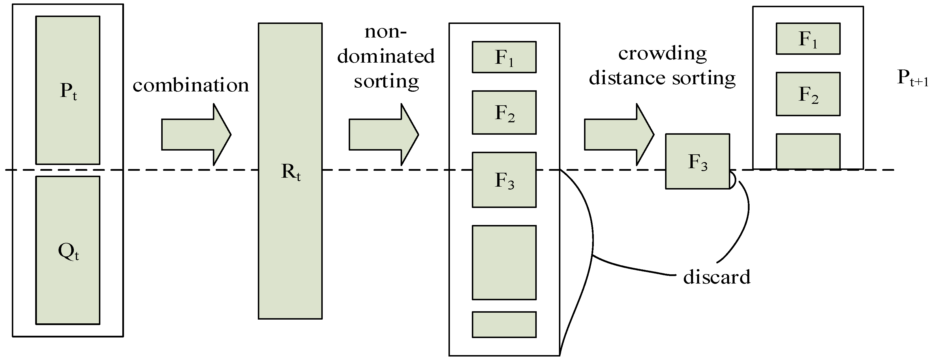
3.5. Cyclic Elimination Strategy of Crowding Distance
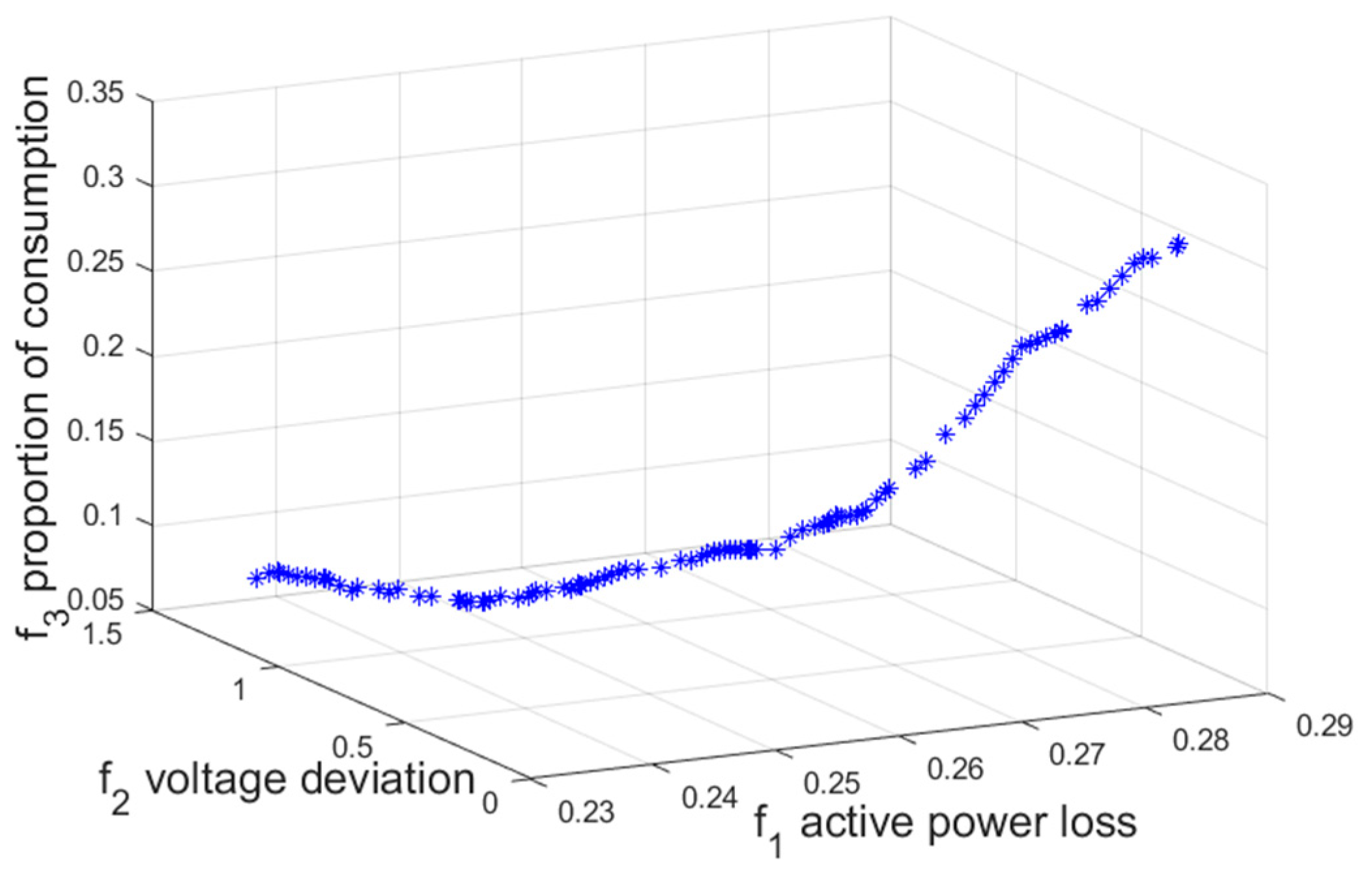
3.6. ISAMOPSO Algorithm Performance Verification and Analysis
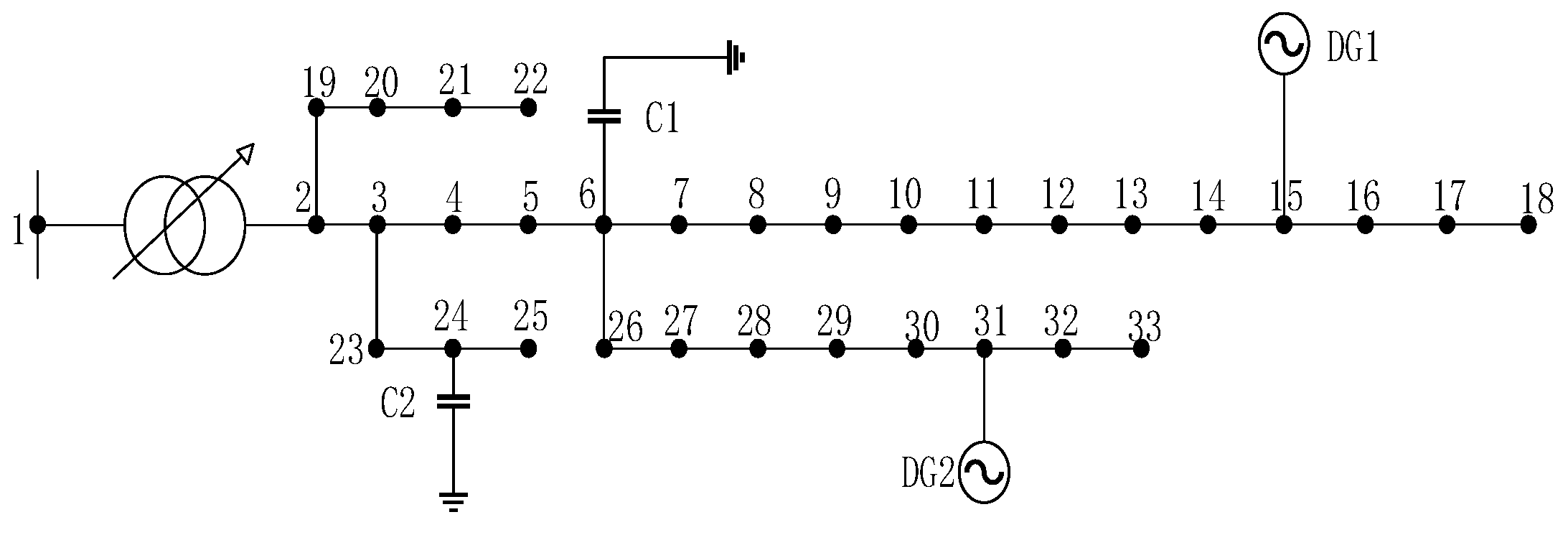
4. Applied ISAMOPSO for Reactive Power Optimization
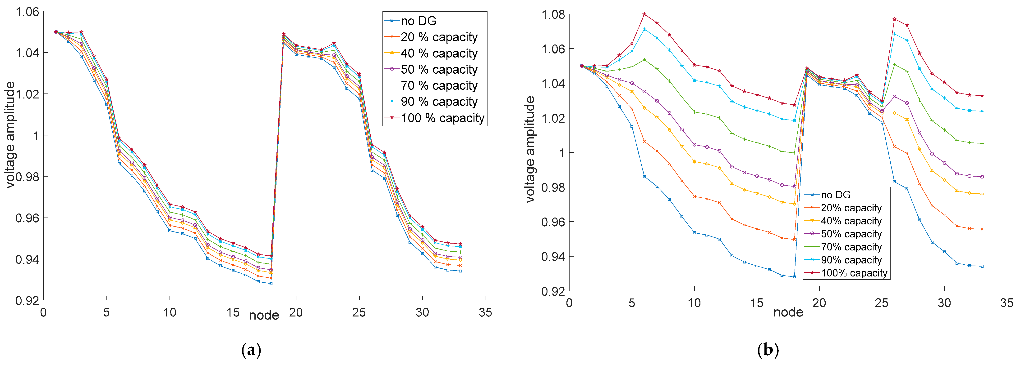
4.1. Influence of Distributed Generation on Distribution Network
4.1.1. Influence of Distributed Generation Capacity on Distribution Network
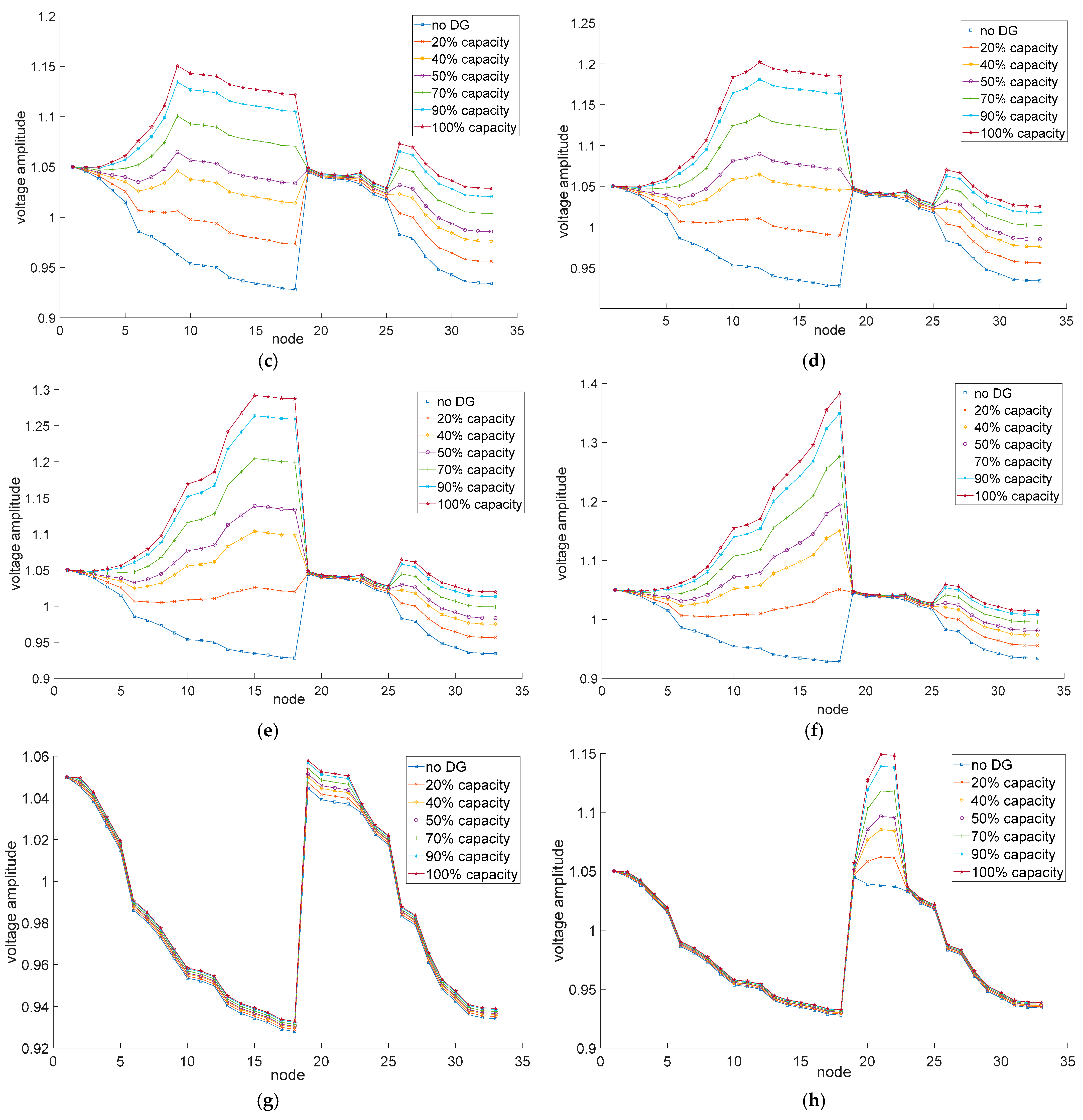
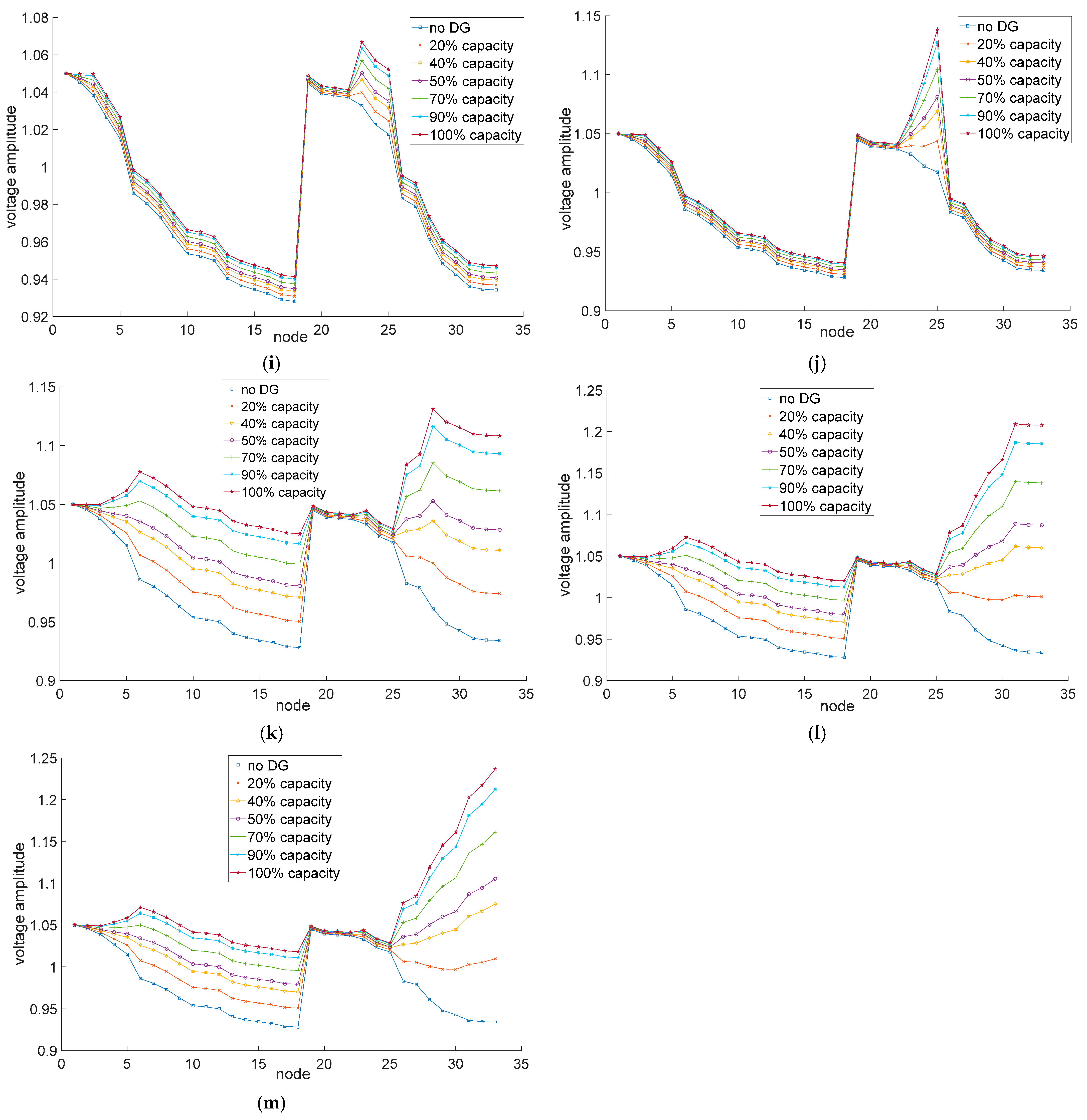
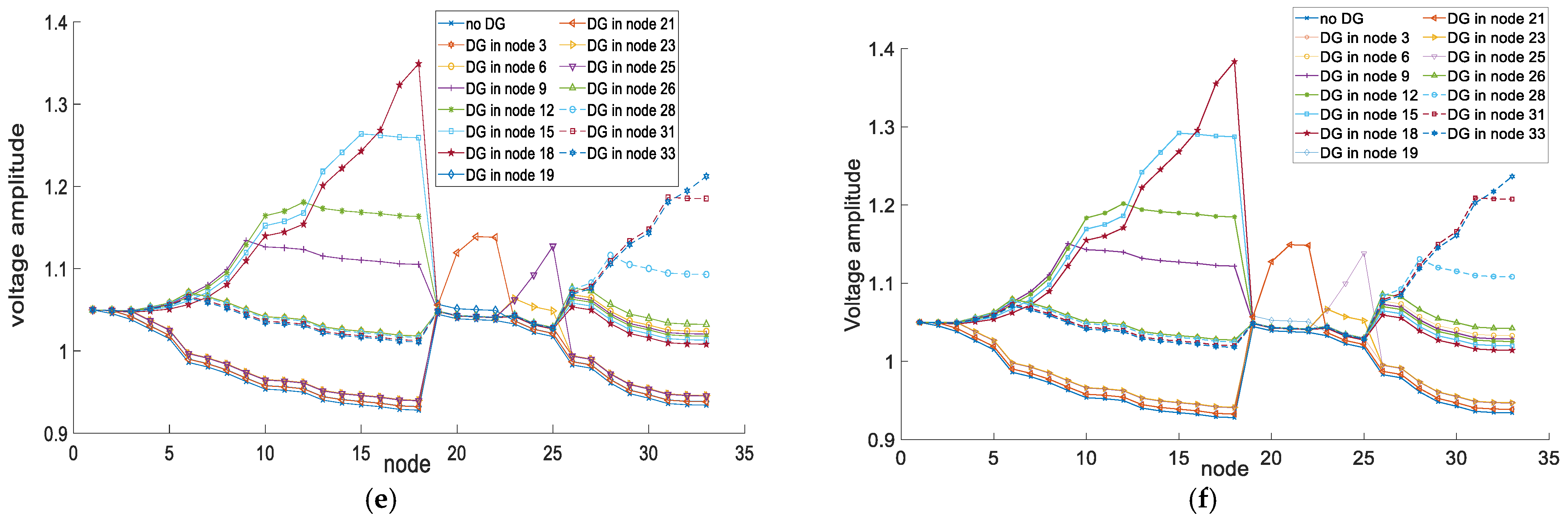
4.1.2. Influence of Distributed Generation Position on Distribution Network
4.2. Multi-Objective Reactive Power Optimization Solution Process
- Step 1: Read the system data, set the population size and the maximum iteration number and the related parameters of the improvement strategy, and initialize the population , personal best and global best .
- Step 2: Update the personal best and leader for each particle. Carry out power flow computation and obtain the objective function values of each particle. The non-dominated solutions of the population are confirmed according to the non-dominated ranking strategy, and the positions of the next generation of particles and the individual optimal positions are updated according to Equation (13).
- Step 3: Generate off-spring population according to Equations (11) and (13) based on the current velocity and position of each particle in , and then combine and together and obtain population whose size is .
- Step 4: Identify the non-dominated solutions from , and store them in .
- Step 5: Generate the particle population for the next iteration and the evaluation criterion Formula (17) for the leader particles.
- Step 6: Based on the state of velocity in the population, determine whether it constitutes a perturbation condition, and adjust the population again.
- Step 7: Determine whether the maximum number of iterations is reached; if so, proceed to the next step; otherwise, go to Step 3 for the next iteration.
- Step 8: Output the non-dominated solutions as the final Pareto-optimal solutions.
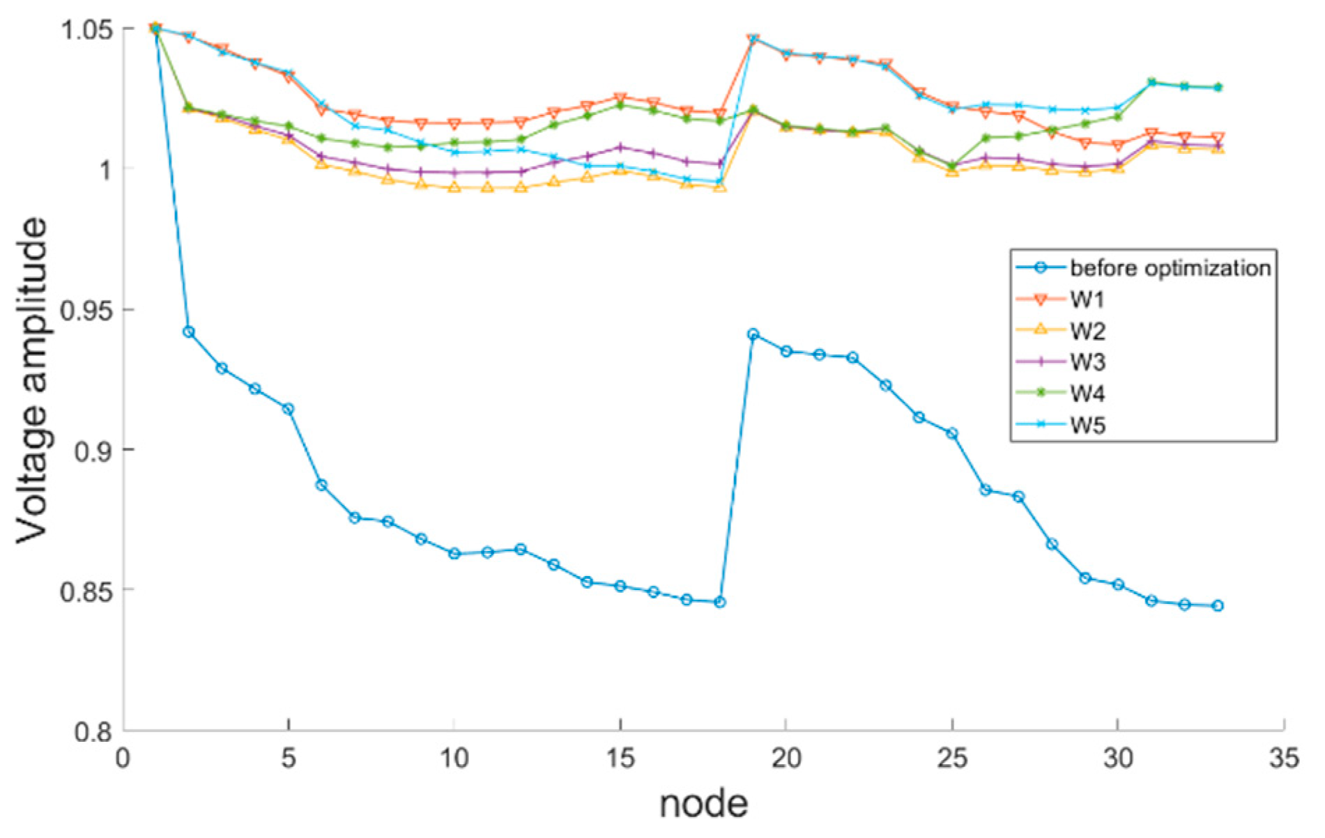
4.3. Analysis and Discussion Results
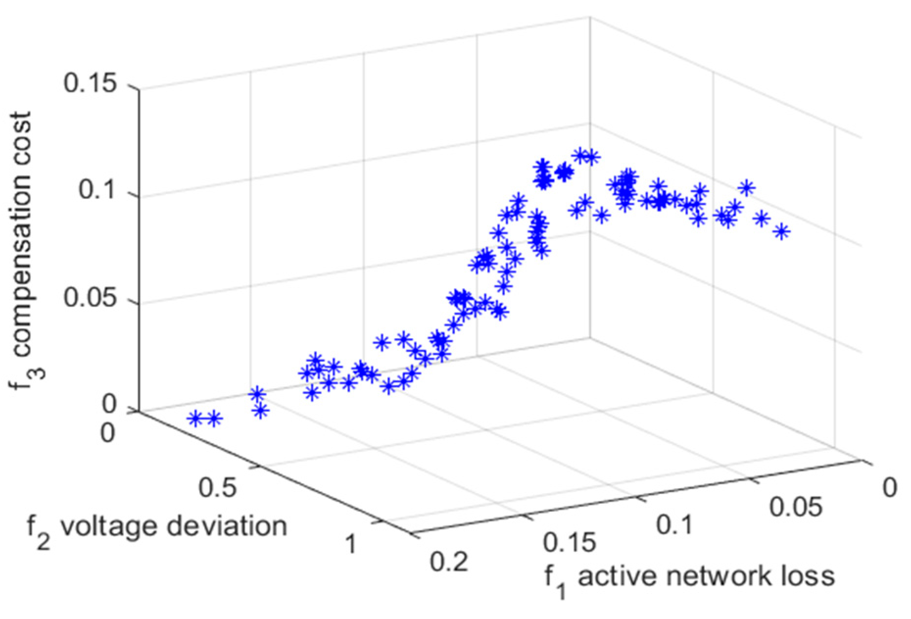
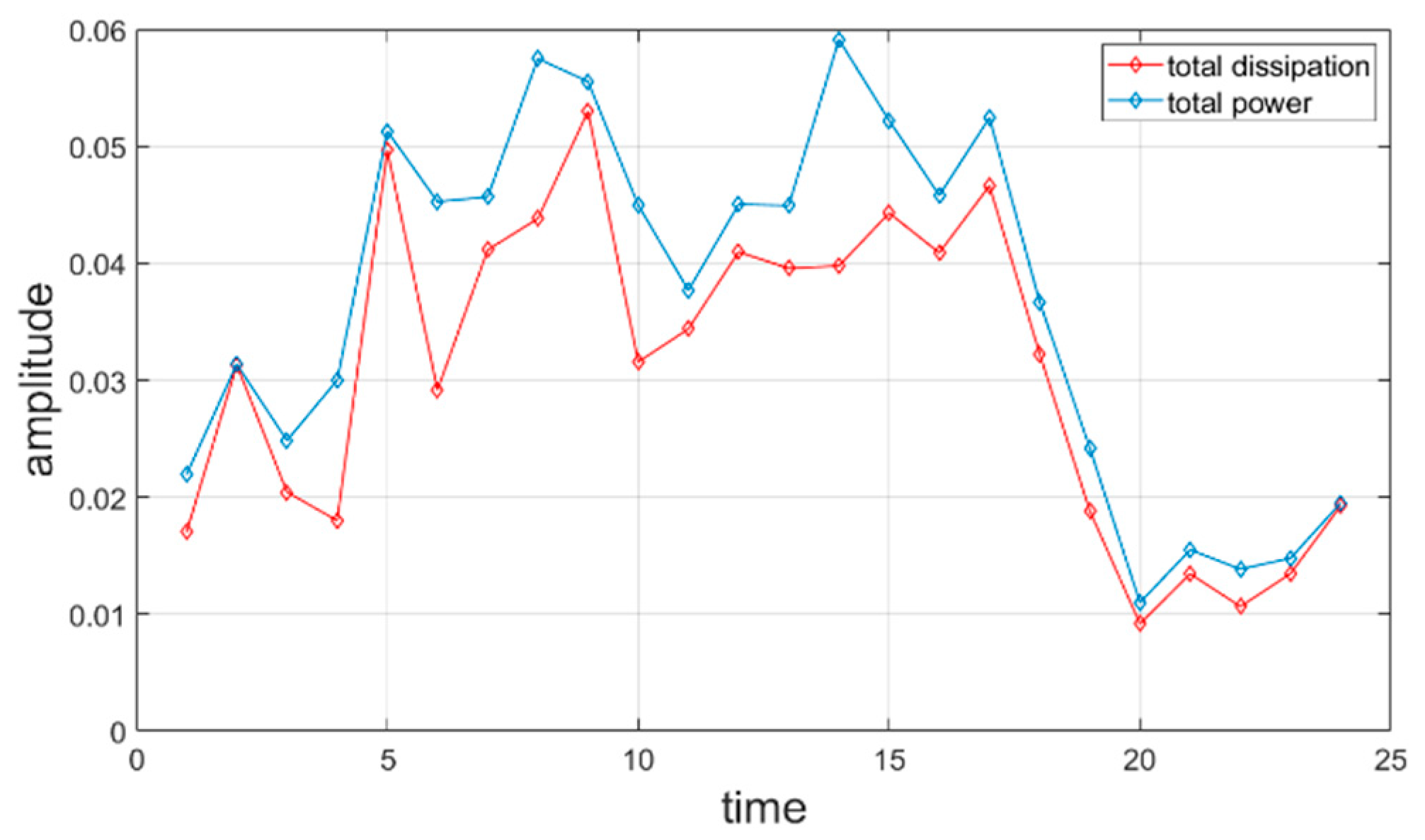
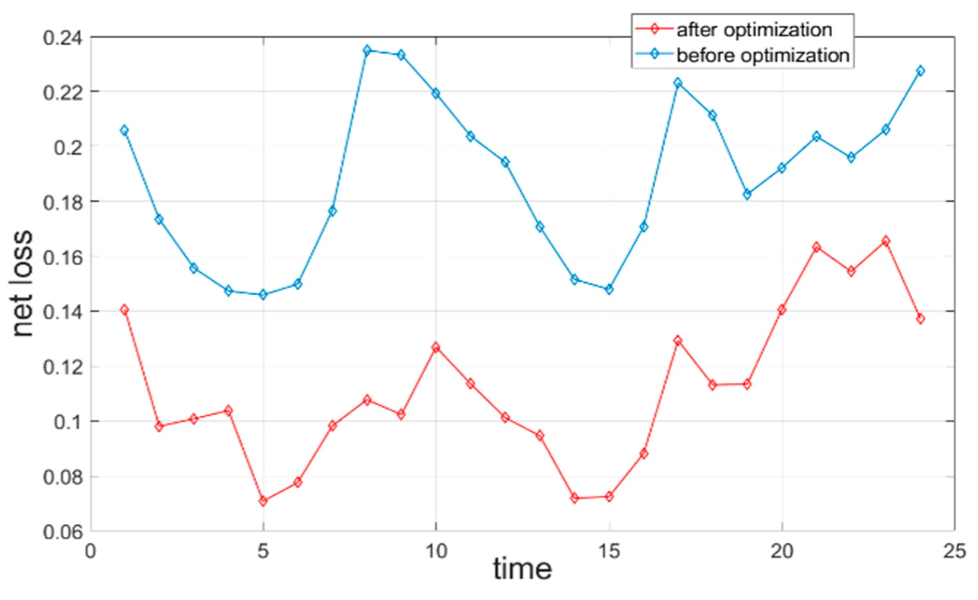
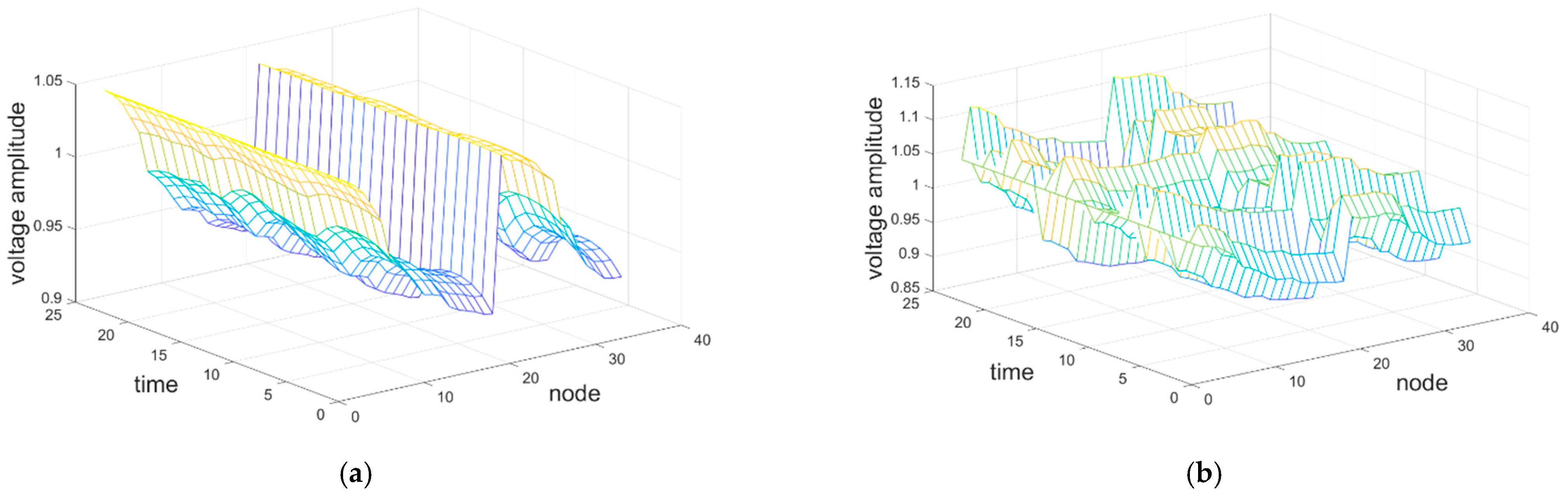
4.3.1. Static Reactive Power Optimization
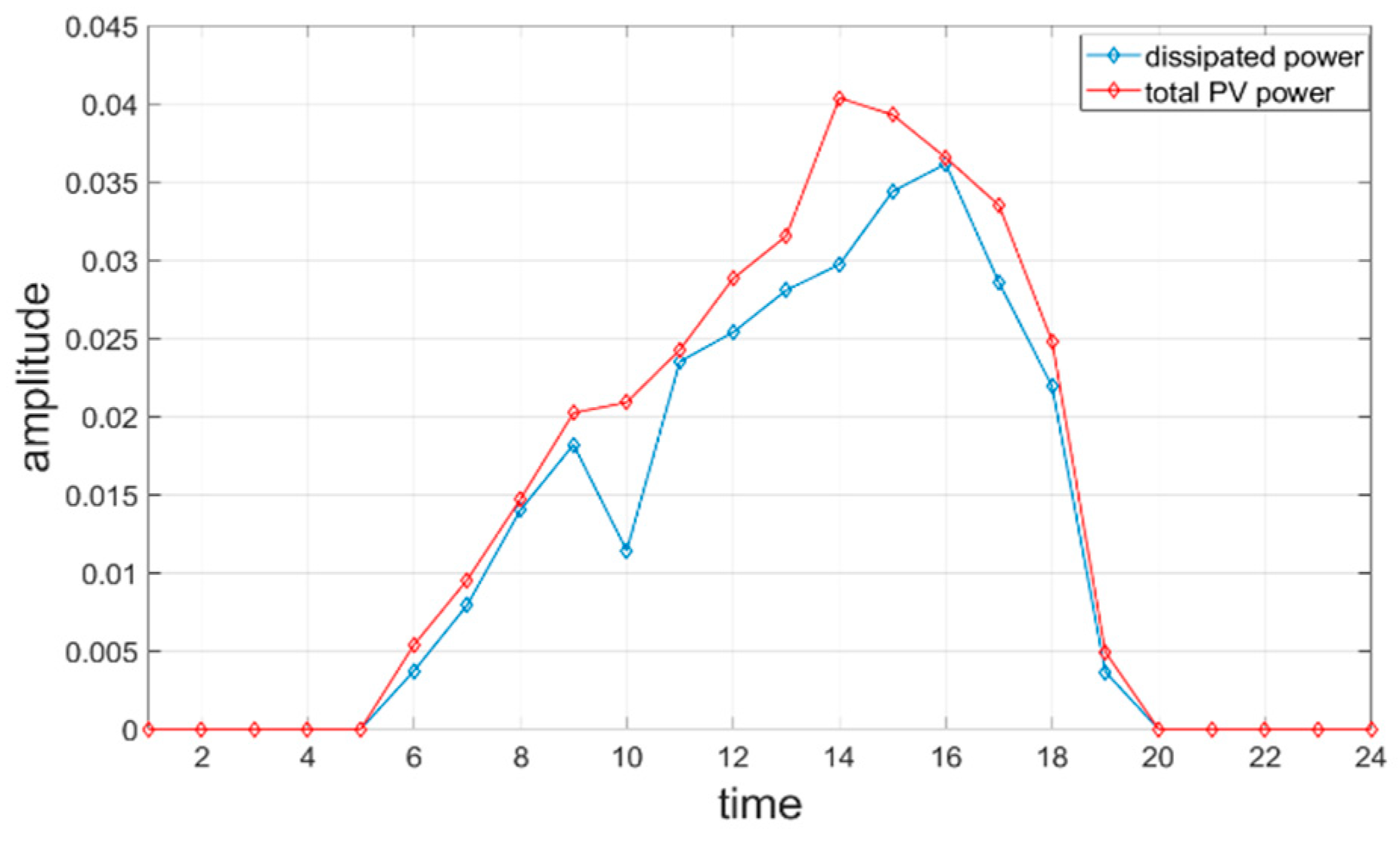
4.3.2. Dynamic Reactive Power Optimization
5. Conclusions
Author Contributions
Funding
Institutional Review Board Statement
Informed Consent Statement
Data Availability Statement
Conflicts of Interest
References
- Diahovchenko, I.; Viacheslav, Z. Optimal composition of alternative energy sources to minimize power losses and maximize profits in a distribution power network. In Proceedings of the 2020 IEEE 7th International Conference on Energy Smart Systems (ESS), Kyiv, Ukraine, 12–14 May 2020; pp. 247–252. [Google Scholar] [CrossRef]
- Ma, W.; Wang, W.; Chen, Z.; Wu, X.; Hu, R.; Tang, F.; Zhang, W. Voltage regulation methods for active distribution networks considering the reactive power optimization of substations. Appl. Energy 2021, 284, 116347. [Google Scholar] [CrossRef]
- Wang, Z.; Liu, H.; Li, J. Reactive Power Planning in Distribution Network Considering the Consumption Capacity of Distributed Generation. In Proceedings of the 2020 5th Asia Conference on Power and Electrical Engineering (ACPEE), Chengdu, China, 4–7 June 2020; pp. 1122–1128. [Google Scholar] [CrossRef]
- Side, D.O.; Picioroaga, I.I.; Tudose, A.M.; Bulac, C.; Tristiu, I. Multi-Objective Particle Swarm optimization Applied on the Optimal Reactive Power Dispatch in Electrical Distribution Systems. In Proceedings of the 2020 International Conference and Exposition on Electrical And Power Engineering (EPE), Iasi, Romania, 22–23 October 2020; pp. 413–418. [Google Scholar] [CrossRef]
- Cheng, X.; Chen, X.; Fan, Y.; Liu, Y.; Li, S.; Zhao, Q. Research on Reactive Power Optimization Control Strategy of Distribution Network with Photovoltaic Generation. In Proceedings of the 2019 Chinese Automation Congress (CAC), Hangzhou, China, 22–24 November 2019; pp. 4026–4030. [Google Scholar] [CrossRef]
- Bi, H. The significance and current situation of reactive power optimization. AIP Conf. Proc. 2019, 2122, 020025. [Google Scholar] [CrossRef]
- Chen, S.; Li, P.; Ji, H.; Yu, H.; Yan, J.; Wu, J.; Wang, C. Operational flexibility of active distribution networks with the potential from data centers. Appl. Energy 2021, 293, 116935. [Google Scholar] [CrossRef]
- Liu, J.; Lu, Y.; Lv, G.; Du, J. Research on Access Point and Capacity Optimization of Distributed Generation in Distribution Power Grid. In Proceedings of the 2021 China International Conference on Electricity Distribution (CICED), Shanghai, China, 7–9 April 2021; pp. 718–721. [Google Scholar] [CrossRef]
- Tonkoski, R.; Lopes, L.A.C.; El-Fouly, T.H.M. Coordinated Active Power Curtailment of Grid Connected PV Inverters for Overvoltage Prevention. IEEE Trans. Sustain. Energy 2021, 2, 139–147. [Google Scholar] [CrossRef]
- Siyuan, C.; Suwen, Z. Research on Reactive Power Optimization Algorithm of Power System Based on Improved Genetic Algorithm. In Proceedings of the 2017 International Conference on Industrial Informatics—Computing Technology, Intelligent Technology, Industrial Information Integration (ICIICII), Wuhan, China, 2–3 December 2017; pp. 21–24. [Google Scholar] [CrossRef]
- Liu, B.; Shi, L.; Yao, Z. Multi-objective optimal reactive power dispatch for distribution network considering pv generation uncertainty. In Proceedings of the 10th Renewable Power Generation Conference (RPG 2021), Online, 14–15 October 2021; pp. 503–509. [Google Scholar] [CrossRef]
- Soldevilla, F.R.C.; Huerta, F.A.C. Minimization of Losses in Power Systems by Reactive Power Dispatch using Particle Swarm Optimization. In Proceedings of the 2019 54th International Universities Power Engineering Conference (UPEC), Bucharest, Romania, 3–6 September 2019; pp. 1–5. [Google Scholar] [CrossRef]
- Srikanth, V.; Natarajan, V.; Jegajothi, B.; Arumugam, S.S.L.D.; Nageswari, D. Fruit fly Optimization with Deep Learning Based Reactive Power Optimization Model for Distributed Systems. In Proceedings of the 2022 International Conference on Electronics and Renewable Systems (ICEARS), Tuticorin, India, 16–18 March 2022; pp. 319–324. [Google Scholar] [CrossRef]
- Ali, M.H.; Kamel, S.; Hassan, M.H.; Tostado-Véliz, M.; Zawbaa, H.M. An improved wild horse optimization algorithm for reliability based optimal DG planning of radial distribution networks. Energy Rep. 2022, 8, 582–604. [Google Scholar] [CrossRef]
- Lian, L. Reactive power optimization based on adaptive multi-objective optimization artificial immune algorithm. Ain Shams Eng. J. 2022, 13, 101677. [Google Scholar] [CrossRef]
- Yuan, Z.; Dou, X.; Wang, L.; Dong, Y. Reactive Power Optimization of Distribution Network Based on BP Neural Network and Intelligent Scene Matching. In Proceedings of the 2021 IEEE Sustainable Power and Energy Conference (iSPEC), Nanjing, China, 23–25 December 2021; pp. 3048–3054. [Google Scholar] [CrossRef]
- Mendes, A.; Boland, N.; Guiney, P.; Riveros, C. (N-1) contingency planning in radial distribution networks using genetic algorithms. In Proceedings of the 2010 IEEE/PES Transmission and Distribution Conference and Exposition: Latin America (T&D-LA), Sao Paulo, Brazil, 8–10 November 2010; pp. 290–297. [Google Scholar] [CrossRef]
- Hui, Q.; Teng, Y.; Zuo, H.; Chen, Z. Reactive power multi-objective optimization for multi-terminal AC/DC interconnected power systems under wind power fluctuation. CSEE J. Power Energy Syst. 2020, 6, 630–637. [Google Scholar] [CrossRef]
- Bo, S.; Yujie, C.; Xiang, Z.; Yelin, W.; Ning, L. Multi-objective reactive power optimization in power system based on improved PSO-OSA algorithm. In Proceedings of the 2019 14th IEEE Conference on Industrial Electronics and Applications (ICIEA), Xi’an, China, 19–21 June 2019; pp. 1514–1519. [Google Scholar] [CrossRef]
- Zhang, C.; Chen, M.; Luo, C. A multi-objective optimization method for power system reactive power dispatch. In Proceedings of the 2010 8th World Congress on Intelligent Control and Automation, Jinan, China, 7–9 July 2010; pp. 6–10. [Google Scholar] [CrossRef]
- Dhifaoui, C.; Guesmi, T.; Welhazi, Y.; Abdallah, H.H. Application of multi-objective PSO algorithm for static reactive power dispatch. In Proceedings of the 2014 5th International Renewable Energy Congress (IREC), Hammamet, Tunisia, 25–27 March 2014; pp. 1–6. [Google Scholar] [CrossRef]
- Zhang, Z.; Wang, X. Optimal Reactive Optimization of Distribution Network with Wind Turbines Based on Improved NSGA-II. In Proceedings of the 2018 China International Conference on Electricity Distribution (CICED), Tianjin, China, 17–19 September 2018; pp. 2056–2060. [Google Scholar] [CrossRef]
- Li, S.; He, Y.; Zhou, Y.; Hu, Y. A New Reactive Power optimization Method For Distribution Network with High Participation of Renewable Distributed Generation. In Proceedings of the 2020 IEEE 4th Conference on Energy Internet and Energy System Integration (EI2), Wuhan, China, 30 October–1 November 2020; pp. 1298–1302. [Google Scholar] [CrossRef]
- Zhang, J.; Liu, K.; Tan, Y.; He, X. Random black hole particle swarm optimization and its application. In Proceedings of the 2008 International Conference on Neural Networks and Signal Processing, Nanjing, China, 7–11 June 2008; pp. 359–365. [Google Scholar] [CrossRef]
- Deb, K.; Pratap, A.; Agarwal, S.; Meyarivan, T. A fast and elitist multiobjective genetic algorithm: NSGA-II. IEEE Trans. Evol. Comput. 2002, 6, 182–197. [Google Scholar] [CrossRef] [Green Version]
- Coello, C.A.C.; Pulido, G.T.; Lechuga, M.S. Handling multiple objectives with particle swarm optimization. IEEE Trans. Evol. Comput. 2004, 8, 256–279. [Google Scholar] [CrossRef]
- Nebro, A.J.; Durillo, J.J.; Garcia-Nieto, J.; Coello, C.A.C.; Luna, F.; Alba, E. SMPSO: A new PSO-based metaheuristic for multi-objective optimization. In Proceedings of the 2009 IEEE Symposium on Computational Intelligence in Multi-Criteria Decision-Making(MCDM), Nashville, TN, USA, 30 March–2 April 2009; pp. 66–73. [Google Scholar] [CrossRef]
- Baran, M.E.; Wu, F.F. Network reconfiguration in distribution systems for loss reduction and load balancing. IEEE Trans. Power Deliv. 1989, 4, 1401–1407. [Google Scholar] [CrossRef]
- Cheng, S.; Chen, M.-Y. Multi-objective reactive power optimization strategy for distribution system with penetration of distributed generation. Int. J. Electr. Power Energy Syst. 2014, 62, 221–228. [Google Scholar] [CrossRef]


| Test Function | Index | Algorithm | |||
|---|---|---|---|---|---|
| NSGAII | MOPSO | SMPSO | ISAMOPSO | ||
| DTLZ1 | Mean | 2.6664 × 10⁻² | 3.1767 × 10⁻² | 3.0328 × 10⁻² | 2.6595 × 10⁻² |
| Std | 1.28 × 10⁻³ | 1.75 × 10⁻² | 1.20 × 10⁻² | 1.09 × 10⁻³ | |
| DTLZ2 | Mean | 6.8392 × 10⁻² | 7.7528 × 10⁻² | 6.6816 × 10⁻² | 6.3912 × 10⁻² |
| Std | 3.38 × 10⁻³ | 8.42 × 10⁻³ | 2.30 × 10⁻³ | 1.79 × 10⁻³ | |
| DTLZ3 | Mean | 6.8458 × 10⁻² | 1.2056 × 10⁻¹ | 6.8460 × 10⁻² | 9.9426 × 10⁻² |
| Std | 2.19 × 10⁻³ | 7.13 × 10⁻² | 2.63 × 10⁻³ | 4.33 × 10⁻² | |
| DTLZ4 | Mean | 6.6723 × 10⁻² | 1.7982 × 10⁻¹ | 1.1460 × 10⁻¹ | 1.5361 × 10⁻¹ |
| Std | 3.02 × 10⁻³ | 1.15 × 10⁻¹ | 1.06 × 10⁻¹ | 1.64 × 10⁻² | |
| DTLZ5 | Mean | 5.7555 × 10⁻³ | 7.7760 × 10⁻³ | 5.3310 × 10⁻³ | 4.8635 × 10⁻³ |
| Std | 3.61 × 10⁻⁴ | 6.66 × 10⁻⁴ | 4.20 × 10⁻⁴ | 1.35 × 10⁻⁴ | |
| DTLZ6 | Mean | 5.7767 × 10⁻³ | 8.5702 × 10⁻³ | 5.3689 × 10⁻³ | 4.6755 × 10⁻³ |
| Std | 2.82 × 10⁻⁴ | 9.20 × 10⁻⁴ | 2.09 × 10⁻⁴ | 9.00 × 10⁻⁵ | |
| DTLZ7 | Mean | 7.9676 × 10⁻² | 1.0997 × 10⁻¹ | 1.0327 × 10⁻¹ | 8.2313 × 10⁻² |
| Std | 6.02 × 10⁻³ | 9.98 × 10⁻² | 3.81 × 10⁻² | 6.18 × 10⁻³ | |
| Function | NSGAⅡ | MOPSO | SMPSO | ISAMOPSO |
|---|---|---|---|---|
| DTLZ1 | 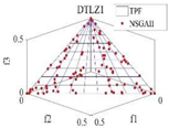 |  |  | 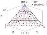 |
| DTLZ2 | 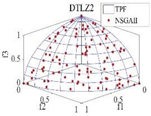 | 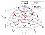 | 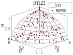 |  |
| DTLZ3 | 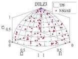 | 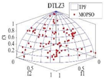 | 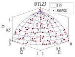 |  |
| DTLZ4 |  |  | 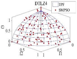 | 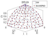 |
| DTLZ5 |  | 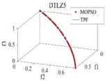 |  |  |
| DTLZ6 | 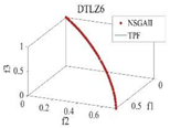 | 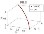 |  | 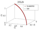 |
| DTLZ7 | 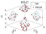 | 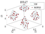 |  | 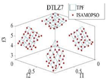 |
| Test Function | Index | Algorithm | |||
|---|---|---|---|---|---|
| NSGAII | MOPSO | SMPSO | ISAMOPSO | ||
| DTLZ1 | Mean | 8.2429 × 10⁻¹ | 7.9694 × 10⁻¹ | 8.1700 × 10⁻¹ | 8.1891 × 10⁻¹ |
| Std | 3.74 × 10⁻³ | 4.61 × 10⁻² | 5.11 × 10⁻³ | 3.13 × 10⁻² | |
| DTLZ2 | Mean | 5.3293 × 10⁻¹ | 5.0980 × 10⁻¹ | 5.3286 × 10⁻¹ | 5.3832 × 10⁻¹ |
| Std | 5.53 × 10⁻³ | 1.29 × 10⁻² | 3.90 × 10⁻³ | 3.56 × 10⁻³ | |
| DTLZ3 | Mean | 5.0795 × 10⁻¹ | 4.6962 × 10⁻¹ | 5.2880 × 10⁻¹ | 5.3488 × 10⁻¹ |
| Std | 5.30 × 10⁻² | 6.38 × 10⁻² | 6.18 × 10⁻³ | 4.64 × 10⁻³ | |
| DTLZ4 | Mean | 5.4192 × 10⁻¹ | 4.9007 × 10⁻¹ | 5.2322 × 10⁻¹ | 5.2573 × 10⁻¹ |
| Std | 3.29 × 10⁻³ | 4.11 × 10⁻² | 3.85 × 10⁻² | 6.46 × 10⁻³ | |
| DTLZ5 | Mean | 1.9930 × 10⁻¹ | 1.9691 × 10⁻¹ | 1.9944 × 10⁻¹ | 1.9965 × 10⁻¹ |
| Std | 1.70 × 10⁻⁴ | 2.61 × 10⁻³ | 2.09 × 10⁻⁴ | 1.25 × 10⁻⁴ | |
| DTLZ6 | Mean | 1.9958 × 10⁻¹ | 1.9781 × 10⁻¹ | 1.9962 × 10⁻¹ | 2.0015 × 10⁻¹ |
| Std | 1.30 × 10⁻⁴ | 4.58 × 10⁻⁴ | 1.74 × 10⁻⁴ | 3.57 × 10⁻⁵ | |
| DTLZ7 | Mean | 2.7128 × 10⁻¹ | 2.6964 × 10⁻¹ | 2.6817 × 10⁻¹ | 2.7167 × 10⁻¹ |
| Std | 1.68 × 10⁻³ | 1.17 × 10⁻² | 2.67 × 10⁻³ | 2.57 × 10⁻³ | |
| Node | 0 | 20% | 40% | 50% | 70% | 90% | 100% |
|---|---|---|---|---|---|---|---|
| 3 | 0.0293 | 0.0228 | 0.022 | 0.0216 | 0.0211 | 0.0208 | 0.0207 |
| 6 | 0.0239 | 0.0159 | 0.011 | 0.0097 | 0.0089 | 0.0104 | 0.012 |
| 9 | 0.0239 | 0.0141 | 0.0107 | 0.011 | 0.0148 | 0.0225 | 0.0276 |
| 12 | 0.0239 | 0.0134 | 0.0118 | 0.0135 | 0.021 | 0.0331 | 0.0405 |
| 15 | 0.0239 | 0.0134 | 0.015 | 0.0189 | 0.0315 | 0.0491 | 0.0595 |
| 18 | 0.0239 | 0.0147 | 0.0198 | 0.0258 | 0.043 | 0.0655 | 0.0785 |
| 19 | 0.0239 | 0.0232 | 0.0229 | 0.0229 | 0.0231 | 0.0237 | 0.0241 |
| 21 | 0.0239 | 0.0237 | 0.0264 | 0.0286 | 0.035 | 0.0434 | 0.0484 |
| 23 | 0.0239 | 0.0224 | 0.0217 | 0.0217 | 0.0223 | 0.0236 | 0.0246 |
| 25 | 0.0239 | 0.0216 | 0.0226 | 0.0243 | 0.0296 | 0.0373 | 0.042 |
| 26 | 0.0239 | 0.0155 | 0.0107 | 0.0094 | 0.009 | 0.0112 | 0.0132 |
| 28 | 0.0239 | 0.0135 | 0.009 | 0.0087 | 0.0111 | 0.0173 | 0.0216 |
| 31 | 0.0239 | 0.0118 | 0.0095 | 0.011 | 0.0185 | 0.0306 | 0.0382 |
| 33 | 0.0239 | 0.0121 | 0.0108 | 0.0131 | 0.022 | 0.0359 | 0.0444 |
| Result | DG1 (Mvar) | DG2 (Mvar) | C1 (Mvar) | C2 (Mvar) | K (pu) | (MW) | (million) | |
|---|---|---|---|---|---|---|---|---|
| W1 | 0.0335 | 0.2965 | 0.15 | 0.15 | 0.975 | 0.0645 | 0.1581 | 0.0594 |
| W2 | 0.1325 | 0.3214 | 0.15 | 0.15 | 0.975 | 0.0663 | 0.1595 | 0.0569 |
| W3 | 0.1618 | 0.2933 | 0.3 | 0.45 | 0.975 | 0.0512 | 0.1287 | 0.0701 |
| W4 | 0.3187 | 0.3396 | 0.45 | 0.75 | 1 | 0.0547 | 0.2741 | 0.0421 |
| W5 | 0.3571 | 0.4163 | 0.45 | 0.3 | 1 | 0.0582 | 0.2803 | 0.0486 |
| Comparison Object | Before Optimization | NSGA-II | ISAMOPSO |
|---|---|---|---|
| (MW) | 0.1885 | 0.0728 | 0.0645 |
| 1.0435 | 0.1945 | 0.1581 | |
| (million) | - | 0.0637 | 0.0594 |
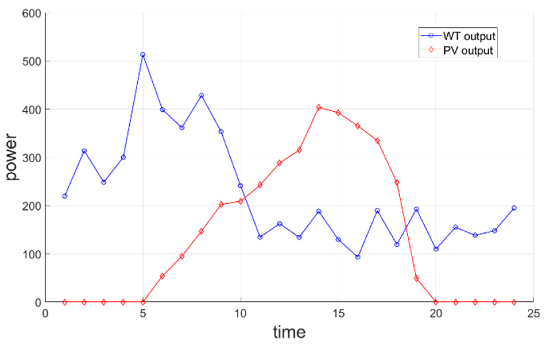
| Time | Light Intensity (W/m2) | Temperature (℃) | Wind Speed (m/s) | PV Output (kW) | WT Output (kW) | Time | Light Intensity (W/m2) | Temperature (℃) | Wind Speed (m/s) | PV Output (kW) | WT Output (kW) |
|---|---|---|---|---|---|---|---|---|---|---|---|
| 0 | 0 | 17.33 | 7.15 | 0 | 219.4 | 12 | 494.44 | 27.46 | 5.90 | 287.9 | 134.3 |
| 1 | 0 | 17.29 | 8.32 | 0 | 313.6 | 13 | 619.44 | 30.10 | 6.72 | 315.1 | 188.1 |
| 2 | 0 | 17.10 | 7.53 | 0 | 248.4 | 14 | 605.56 | 29.26 | 5.82 | 403.4 | 129.5 |
| 3 | 0 | 16.73 | 8.16 | 0 | 299.9 | 15 | 565.56 | 29.18 | 5.18 | 392.7 | 93.01 |
| 4 | 0 | 16.32 | 10.37 | 0 | 513 | 16 | 522.22 | 28.35 | 6.74 | 365.2 | 189.8 |
| 5 | 91.67 | 16.06 | 9.25 | 0 | 399 | 17 | 394.44 | 26.30 | 5.65 | 334.8 | 119.2 |
| 6 | 161.11 | 16.11 | 8.86 | 53.78 | 361.6 | 18 | 81.67 | 23.93 | 6.78 | 247.9 | 192.6 |
| 7 | 245.56 | 16.66 | 9.55 | 95.25 | 428.3 | 19 | 0 | 21.55 | 5.48 | 49.25 | 109.8 |
| 8 | 333.33 | 17.90 | 8.77 | 146.8 | 353.4 | 20 | 0 | 19.50 | 6.22 | 0 | 154.9 |
| 9 | 341.67 | 19.91 | 7.43 | 202.1 | 241 | 21 | 0 | 18.03 | 5.96 | 0 | 138.3 |
| 10 | 391.11 | 22.42 | 5.90 | 208.8 | 134.5 | 22 | 0 | 17.09 | 6.11 | 0 | 147.7 |
| 11 | 457.22 | 25.05 | 6.34 | 242.4 | 162.4 | 23 | 0 | 16.52 | 6.81 | 0 | 194.9 |
Publisher’s Note: MDPI stays neutral with regard to jurisdictional claims in published maps and institutional affiliations. |
© 2022 by the authors. Licensee MDPI, Basel, Switzerland. This article is an open access article distributed under the terms and conditions of the Creative Commons Attribution (CC BY) license (https://creativecommons.org/licenses/by/4.0/).
Share and Cite
Song, J.; Lu, C.; Ma, Q.; Zhou, H.; Yue, Q.; Zhu, Q.; Zhao, Y.; Fan, Y.; Huang, Q. Distributed Integrated Synthetic Adaptive Multi-Objective Reactive Power Optimization. Symmetry 2022, 14, 1275. https://doi.org/10.3390/sym14061275
Song J, Lu C, Ma Q, Zhou H, Yue Q, Zhu Q, Zhao Y, Fan Y, Huang Q. Distributed Integrated Synthetic Adaptive Multi-Objective Reactive Power Optimization. Symmetry. 2022; 14(6):1275. https://doi.org/10.3390/sym14061275
Chicago/Turabian StyleSong, Jiayin, Chao Lu, Qiang Ma, Hongwei Zhou, Qi Yue, Qinglin Zhu, Yue Zhao, Yiming Fan, and Qiqi Huang. 2022. "Distributed Integrated Synthetic Adaptive Multi-Objective Reactive Power Optimization" Symmetry 14, no. 6: 1275. https://doi.org/10.3390/sym14061275
APA StyleSong, J., Lu, C., Ma, Q., Zhou, H., Yue, Q., Zhu, Q., Zhao, Y., Fan, Y., & Huang, Q. (2022). Distributed Integrated Synthetic Adaptive Multi-Objective Reactive Power Optimization. Symmetry, 14(6), 1275. https://doi.org/10.3390/sym14061275