A Subgradient-Type Extrapolation Cyclic Method for Solving an Equilibrium Problem over the Common Fixed-Point Sets

Abstract

In this paper, we consider the solving of an equilibrium problem over the common fixed set of cutter mappings in a real Hilbert space. To this end, we present a subgradient-type extrapolation cyclic method. The proposed method is generated based on the ideas of a subgradient method and an extrapolated cyclic cutter method. We prove a strong convergence of the method provided that some suitable assumptions of step-size sequences are assumed. We finally show the numerical behavior of the proposed method.

1. Introduction

Let $\mathcal{H}$ be a real Hilbert space with inner product $⟨·,·⟩$ and its induced norm $\parallel ·\parallel$. In this paper, we present an iterative method to the equilibrium problem over the intersection of fixed-point set:

Problem 1 (BEP).

Let $T_i:\mathcal{H}\to \mathcal{H}$, $i=1,2,\dots ,m$, be cutters with ${\displaystyle \bigcap _{i=1}^m}Fix{T}_i\ne \varnothing$, and let $f:\mathcal{H}\times \mathcal{H}\to \mathbb{R}$ be a bifunction satisfying $f(x,x)=0$ for all $x\in \mathcal{H}$. Then, our objective is to find a point $\overline{u}\in \bigcap _{i=1}^{m}Fix{T}_i$ such that

$$f(\overline{u},y)\ge 0\mathrm{for}\mathrm{all}y\in \bigcap _{i=1}^{m}Fix{T}_i,$$

where $Fix{T}_i:=\{x\in \mathcal{H}:T_{i}x=x\}$ denotes the set of fixed points of $T_i$.

The equilibrium problem, which was first introduced by Fan [1], includes many problems as particular cases, for example, the fixed-point problem, the variational inequality, the optimization problem, the saddle point problem, the Nash equilibrium problem in non-cooperative games, and others; see, for instance, [2,3,4,5] and references therein.

The equilibrium problems over the fixed-point set have been considered in many articles; see, for instance, [6,7,8,9,10] and references therein. The computational algorithms for solving these kinds of problems have been studied and developed by using the idea of the methods for equilibrium problems and the iterative schemes for fixed-point problems. In particular, Iiduka and Yamada [6] considered the equilibrium problems over the fixed-point set of a firmly nonexpansive mapping and presented a subgradient-type method for solving the considered problems. They showed the convergence of their method and applied the method to the Nash equilibrium problems. After that, the equilibrium problems over the common fixed-point of nonexpansive mappings were considered by Duc and Muu in [7]. They proposed the splitting algorithm, which was updated based on the idea of the classical gradient method and the Krasnosel’skii–Mann method and presented the strong convergence of the presented algorithm. Recently, Thuy and Hai [8] considered the bilevel equilibrium problems and proposed the projected subgradient algorithm to solve the considered problem. They exhibited the strong convergence of the proposed method and applied it to the equilibrium problems over the fixed-point set of a nonexpansive mapping. We notice that the aforementioned literature is considered in the case of the equilibrium problems over the fixed-point set of nonexpansive mappings.

Let us focus on the constrained set of BEP. Now, let $T_i:\mathcal{H}\to \mathcal{H}$, $i=1,2,\dots ,m$, be cutter operators. The common fixed-point problem is to find a point

$$x^{*}\in \bigcap _{i=1}^{m}Fix{T}_i\ne \varnothing$$

The well-known methods of finding a point that belongs to the intersection of fixed-point sets are initially motivated by the cyclic projection method, which was introduced by Kaczmarz [11]. After that, the convergence of cyclic projection-type methods are investigated in several directions and their convergence results are guaranteed under the operators’ assumptions, such as cutters or nonexpansive operators, see [12,13,14,15,16] and references therein. In particular, Bauschke and Combettes [17] proposed the cyclic cutter method and showed a weak convergence of the proposed method. In [18], Cegielski and Censor presented the extrapolated cyclic cutter method, which is an acceleration of the cyclic cutter method by imposing an appropriate step-size function to the method. Indeed, let $T_i:\mathcal{H}\to \mathcal{H}$, $i=1,2,\dots ,m$, be cutters with ${\displaystyle \bigcap _{i=1}^m}Fix{T}_i\ne \varnothing$, we define the step-size function $\sigma :\mathcal{H}\to (0,\infty )$ as follows:

$$\sigma \left(x\right):=\left\{\begin{array}{cc}{\displaystyle \frac{{\sum }_{i=1}^m⟨Tx-S_{i-1}x,S_{i}x-S_{i-1}x⟩}{{\parallel Tx-x\parallel }^2},}\hfill & \mathrm{for}x\notin \bigcap _{i=1}^{m}Fix{T}_i,\hfill \\ 1,\hfill & \mathrm{otherwise},\hfill \end{array}\right.$$

(1)

where the operator T, $S_0$ and $S_i,i=1,2,\dots ,m$ are defined as

$$\begin{array}{c}\hfill T:=T_m{T}_{m-1}\cdots T_1, S_0: = Id, \mathrm{and} S_i: = T_i{T}_{i-1}\cdots T_1.\end{array}$$

(2)

It was shown that the extrapolated cyclic cutter method weakly converges provided that the cutter operators $T_i$ satisfied the demi-closedness principle for all $i=1,2,\dots ,m$. Note that, for some practical problem, the value of the extrapolation function may be huge, which lead to some numerical instabilities. To keep away from these instabilities, Cegielski and Nimana [19] proposed the modified extrapolated subgradient projection method for solving the convex feasibility problem, which is a particular situation of common fixed-point problem, and established the convergence of the proposed method as well as demonstrated the performance of the method by the numerical results. After that, the authors in [20] also utilized the idea of the extrapolated cyclic cutter method for dealing with the variational inequality problem with common fixed-point constraints. It can be noted that from [19,20], the iterative methods with extrapolated cyclic cutter terms achieve not only some numerical superiorities to utilizing the classical cyclic cutter scheme but also guarantee the boundedness of the generated sequence, see [20] for further discussions.

In this paper, we propose an iterative algorithm called the Subgradient-type extrapolation cyclic method for solving the equilibrium problems over the intersection of fixed-point sets of cutter operators. The proposed algorithm can be considered as a combination of the subgradient iterative scheme for equilibrium problems in [8] and the extrapolated cyclic cutter method for the intersection of fixed-point sets of cutter operators in [18]. Using the cutter operators and assumptions, we investigate the convergence of the presented algorithm. Moreover, we also present a numerical result of our presented method to illustrate the efficiency of the method.

This paper is organized as follows. In Section 2, we recall some definitions and tools which are needed for our convergence work. In Section 3, we present the subgradient-type extrapolation cyclic method for finding the solution of BEP. We subsequently present the convergence result in this section. In Section 4, the efficacy of the subgradient-type extrapolation cyclic method is illustrated by numerical experiments of the solving equilibrium problem governed by the positive definite symmetric matrices over the common fixed-point set. Finally, we give some concluding remarks in Section 5.

2. Preliminaries

In section, we collect some basic definitions, properties, and useful tools for our work. The readers can consult the books [16,21] for more details.

We denote by $Id$ the identity operator on a real Hilbert space $\mathcal{H}$. For a sequence ${\left\{x^n\right\}}_{n=1}^{\infty }$, the strong and weak convergences of a sequence ${\left\{x^n\right\}}_{n=1}^{\infty }$ to a point $x\in \mathcal{H}$ are defined by the expression $x^n\to x$ and $x^n\rightharpoonup x$, respectively.

In what follows, we recall some definitions and properties of the operator that will be referred to in our analysis.

Definition 1

([16]). Let $T:\mathcal{H}\to \mathcal{H}$ be an operator having a fixed point. The operator T is called

(i)

quasi-nonexpansive, if

$$\parallel Tx-z\parallel \le \parallel x-z\parallel ,$$

for all $x\in \mathcal{H}$ and $z\in FixT,$

(ii)

η-strongly quasi-nonexpansive, if there exists $\eta \ge 0$,

$$\parallel Tx-z{\parallel }^2\le {\parallel x-z\parallel }^2-\eta {\parallel Tx-x\parallel }^2,$$

for all $x\in \mathcal{H}$ and $z\in FixT$,

(iii)

cutter, if

$$⟨x-Tx,z-Tx⟩\le 0,$$

for all $x\in \mathcal{H}$ and $z\in FixT.$

Lemma 1

[16] (Remark 2.1.31 and Theorem 2.1.39). Let $T:\mathcal{H}\to \mathcal{H}$ be an operator having a fixed point. Then the following statements are equivalent:

(i)

T is cutter.

(i)

$⟨Tx-x,z-x⟩\ge \parallel Tx-x{\parallel }^2$ for all $x\in \mathcal{H}$ and for all $z\in FixT$.

(ii)

T is 1-strongly quasi-nonexpansive.

Definition 2

[16] (Definition 3.2.6). Let $T:\mathcal{H}\to \mathcal{H}$ be an operator having a fixed point. The operator T is said to satisfy the demi-closedness (DC) principle if for every sequence $\left\{x^n\right\}\subset \mathcal{H}$, $x^n\rightharpoonup u\in \mathcal{H}$ and $\parallel T{x}^n-x^n\parallel \to 0$, we have $u\in FixT$.

Definition 3

[16] (Definition 2.1.2). Let $T:\mathcal{H}\to \mathcal{H}$ be an operator and $\lambda \in [0,2]$ be given. We define the relaxation of the operator T by

$$T_{\lambda }:=(1-\lambda )Id+\lambda T,$$

and we call λ a relaxation parameter.

Next, we recall the definition of a generalization of relaxation of an operator.

Definition 4

[16] (Definition 2.4.1). Let $T:\mathcal{H}\to \mathcal{H}$ be an operator, $\lambda \in [0,2]$ and $\sigma :\mathcal{H}\to (0,\infty )$. We define the operator $T_{\sigma ,\lambda }:\mathcal{H}\to \mathcal{H}$ by

$$T_{\sigma ,\lambda }x:=x+\lambda \sigma \left(x\right)(Tx-x).$$

This operator T is called a generalized relaxation of the operator T, the value λ is called a relaxation parameter and the function σ is called a step-size function. The operator $T_{\sigma ,\lambda }$ is called an extrapolation of $T_{\lambda }$ if the function $\sigma \left(x\right)\ge 1$ for every $x\in \mathcal{H}$.

We notice that, if $\sigma \left(x\right)=1$, for every $x\in \mathcal{H}$, then $T_{\sigma ,\lambda }=T_{\lambda }$. Note that $T_{\sigma }: =T_{\sigma ,1}$. Then, for every $x\in \mathcal{H}$, the following relations hold

$$\begin{array}{c}\hfill T_{\sigma ,\lambda }x-x=\lambda \sigma \left(x\right)(Tx-x)=\lambda (T_{\sigma }x-x),\end{array}$$

(3)

and for any $\lambda \ne 0$, we have

$$Fix{T}_{\sigma ,\lambda }=Fix{T}_{\sigma }=FixT.$$

Next, we provide an important lemma of the step-size function for proving the convergence result.

Lemma 2

[16] (Section 4.10). Let $T_i:\mathcal{H}\to \mathcal{H},i=1,2,\dots ,m,$ be cutters with ${\displaystyle \bigcap _{i=1}^m}Fix{T}_i\ne \varnothing$ and denote the operator T, $S_0$ and $S_i,i=1,2,\dots ,m$ as in (2). Let the function $\sigma :\mathcal{H}\to (0,\infty )$ be given by (1). Then the following statements are true:

(i)

For every $x\notin FixT$, it is true that

$$\sigma \left(x\right)\ge \frac{\frac{1}{2}{\sum }_{i=1}^m\parallel S_{i}x-S_{i-1}x{\parallel }^2}{\parallel Tx-x{\parallel }^2}\ge \frac{1}{2m}.$$

(ii)

The operator $T_{\sigma }$ is a cutter.

Now, we recall a notion and some properties of a diagonal subdifferential which will be used in this work.

A function $h:\mathcal{H}\to \mathbb{R}$ is said to be subdifferentiable at $x^0\in \mathcal{H}$ if there exists a vector $w\in \mathcal{H}$ such that

$$h\left(x\right)\ge h\left(x^0\right)+⟨w,x-x^0⟩,\forall x\in \mathcal{H}.$$

The vector w is called a subgradient of the function h at $x^0$. The collection of all such vectors constitute the subdifferential of h at $x^0$ and is denoted by $\partial h\left(x^0\right).$

Let $f:\mathcal{H}\times \mathcal{H}\to \mathbb{R}$ be a bifunction which is convex in the second argument, that is, the function $f(x,·):\mathcal{H}\to \mathbb{R}$ is convex at x, for all $x\in \mathcal{H}.$ Then, the set of all subgradient of $f(x,·)$ at x is called the diagonal subdifferential and is denoted by ${\partial }_{2}f(x,x):=\partial f(x,·)\left(x\right)$. The reader can find the notion of the diagonal subdifferential in [22], for more detail.

We end this section by recalling some technical lemmas that are important tools in proving our convergence result.

Lemma 3

[23] (Lemma 3.1). Let ${\left\{a_n\right\}}_{n=1}^{\infty }$ and ${\left\{b_n\right\}}_{n=1}^{\infty }$ be sequences of nonnegative real numbers such that

$$a_{n+1}\le a_n+b_n.$$

If $\sum _{n=1}^{\infty }{b}_n<\infty$, then $\underset{n\to \infty }{lim}{a}_n$ exists.

Lemma 4

[24] (Lemma 3.1). Let ${\left\{a_n\right\}}_{n=1}^{\infty }$ be a sequence of real numbers such that there exists a subsequence ${\left\{a_{n_j}\right\}}_{j=1}^{\infty }$ of ${\left\{a_n\right\}}_{n=1}^{\infty }$ with $a_{n_j}<a_{n_{j+1}}$ for all $j\in \mathbb{N}$. If, for all $n\ge n_0$, we define

$$\nu \left(n\right)=max\left\{k\in [n_0,n]:a_k<a_{k+1}\right\},$$

then the following hold:

(i)

${\left\{\nu \left(n\right)\right\}}_{n\ge n_0}$ is non-decreasing.

(ii)

$\underset{n\to \infty }{lim}\nu \left(n\right)=\infty$.

(iii)

$a_{\nu \left(n\right)}\le a_{\nu \left(n\right)+1}$ and $a_n\le a_{\nu \left(n\right)+1}$ for every $n\ge n_0$.

3. Algorithm and Its Convergence Result

In this section, we firstly propose the subgradient-type extrapolation cyclic method for solving BEP. Subsequently, we present useful lemmas and prove the main convergence theorem.

Remark 1.

(i)

When the number $m=1$ and $\sigma \left(x^n\right)=1$, Algorithm 1 becomes Algorithm 2 considered in [8]. Moreover, it is worth noting that the class of operator considered in this work is different from [8]. In fact, we consider the cutter property of $T_i$, whereas the nonexpansiveness of T is assumed in [8].

(ii)

If the function $f(·,·)=0$, Algorithm 1 is reduced to

$$x^{n+1}=x^n-\frac{{\lambda }_n}{{\eta }_n}\sigma \left(x^n\right)(x^n-T{x}^n),$$

where ${\eta }_n=max\{\mu ,\parallel d^n\parallel \}$ for all $n\ge 1$. In the case when ${\eta }_n=1$ for all $n\ge 1$, this scheme is related to the extrapolated cyclic cutter proposed by [18]. Moreover, this scheme is also related to the work of Cegielski and Nimana [19] for solving a convex feasibility problem when the operator $T_m$ is omitted in their paper.

The following assumption relating to the convergence of Algorithm 1 is assumed throughout this work.

Algorithm 1: Subgradient-type extrapolation cyclic method

Initialization: Given the positive real sequences ${\left\{{\alpha }_n\right\}}_{n=1}^{\infty }$ and ${\left\{{\lambda }_n\right\}}_{n=1}^{\infty }$. Choose $\mu \in (0,+\infty )$ and $x^1\in \mathcal{H}$ arbitrarily. Step 1. For given $x^n\in \mathcal{H}$, compute the step size as $$\sigma \left(x^n\right):=\left\{\begin{array}{cc}{\displaystyle \frac{{\sum }_{i=1}^m⟨T{x}^n-S_{i-1}{x}^n,S_i{x}^n-S_{i-1}{x}^n⟩}{\parallel T{x}^n-x^n{\parallel }^2},}\hfill & \mathrm{for}{x}^n\notin {\displaystyle \bigcap _{i=1}^m}Fix{T}_i,\hfill \\ 1,\hfill & \mathrm{otherwise}.\hfill \end{array}\right.$$ Step 2. Update the next iterate $x^{n+1}$ as $$\begin{array}{ccc}\hfill d^n& : =& \sigma \left(x^n\right)(x^n-T{x}^n)+{\alpha }_n{w}^n;\mathrm{where}{w}^n\in {\partial }_{2}f(x^n,x^n),\hfill \\ \hfill {\eta }_n& : =& max\{\mu ,\parallel d^n\parallel \},\hfill \\ \hfill x^{n+1}& : =& x^n-\frac{{\lambda }_n}{{\eta }_n}{d}^n.\hfill \end{array}$$ Put $n: =n+1$ and go to Step 1.

Assumption A1.

Assume that

(A1)

The bifunction f is ρ-strongly monotone on $\mathcal{H}$, that is, there exists a constant $\rho >0$ satisfying

$$f(x,y)+f(y,x)\le -\rho {\parallel x-y\parallel }^2,\forall x,y\in \mathcal{H}.$$

(A2)

For each $x\in \mathcal{H}$, the function $f(x,·)$ is convex, subdifferentiable and lower semicontinuous on $\mathcal{H}$.

(A3)

The function $x\mapsto {\partial }_{2}f(x,x)$ is bounded on a bounded subset of $\mathcal{H}$.

(A4)

The sequences ${\left\{{\lambda }_n\right\}}_{n=1}^{\infty }$ and ${\left\{{\alpha }_n\right\}}_{n=1}^{\infty }$ satisfy ${\displaystyle \sum _{n=1}^{\infty }}{\lambda }_n=\infty$, ${\displaystyle \sum _{n=1}^{\infty }}{\lambda }_n^2<\infty$, ${\displaystyle \sum _{n=1}^{\infty }}{\alpha }_n{\lambda }_n=\infty$, and $\underset{n\to \infty }{lim}{\alpha }_n=0$.

Remark 2.

(i)

If the whole space $\mathcal{H}$ is finite dimensional, the assumption that, for all $x\in \mathcal{H}$, the function $f(x,·)$ is subdifferentiable and weakly lower semicontinuous in (A2) can be omitted. This is because, in the finite dimensional setting, the convexity implies the continuity of a function.

(ii)

The convexity of the function $f(x,·)$ implies that the lower semicontinuity is equivalent to the weak lower semicontinuity of the function $f(x,·)$ for all $x\in \mathcal{H}$.

(iii)

If the whole space $\mathcal{H}$ is finite dimensional, by invoking the assumption (A2), we have the diagonal subdifferential ${\partial }_{2}f(x^n,x^n):=\partial f(x^n,·)\left(x^n\right)$ is nonempty for all $n\in \mathbb{N}$. Moreover, in this case, the assumption (A3) can be omitted, see [21] (Proposition 16.20).

(iv)

An example of the corresponding step-size sequences in (A4) is the positive real sequences ${\left\{{\alpha }_n\right\}}_{n=1}^{\infty }$ and ${\left\{{\lambda }_n\right\}}_{n=1}^{\infty }$ given by

$${\alpha }_n: =\frac{\alpha }{{(n+1)}^a}\mathrm{and}{\lambda }_n: =\frac{\lambda }{{(n+1)}^b},$$

where $\alpha ,\lambda >0$ and $a,b>0$ with $b>0.5$ and $a+b\le 1$. In fact, since $0<a+b\le 1$ and $b>0.5$, we have $0.5<b<1$ and then ${\sum }_{n=1}^{\infty }{\lambda }_n={\sum }_{n=1}^{\infty }\frac{\lambda }{{(n+1)}^b}>\lambda {\sum }_{n=1}^{\infty }\frac{1}{(n+1)}=\infty$. Furthermore, since $1<2b<2$, we have ${\sum }_{n=1}^{\infty }{\lambda }_n^2={\sum }_{n=1}^{\infty }\frac{{\lambda }^2}{{(n+1)}^{2b}}<\infty$. We note that ${\sum }_{n=1}^{\infty }{\alpha }_n{\lambda }_n={\sum }_{n=1}^{\infty }\frac{\alpha }{{(n+1)}^a}\frac{\lambda }{{(n+1)}^b}=\alpha \lambda {\sum }_{n=1}^{\infty }\frac{1}{{(n+1)}^{a+b}}=\infty$. Moreover, we have that $\underset{n\to \infty }{lim}{\alpha }_n=\underset{n\to \infty }{lim}\frac{\alpha }{{(n+1)}^a}=0$.

The following lemma states the important relation of the generated iterates.

Lemma 5.

Let ${\left\{x^n\right\}}_{n=1}^{\infty }$ be the sequence generated by Algorithm 1. Then, for every $n\in \mathbb{N}$ and $u\in {\bigcap }_{i=1}^{m}Fix{T}_i$, it holds that

$${\parallel x^{n+1}-u\parallel }^2\le {\parallel x^n-u\parallel }^2-\frac{{\lambda }_n}{4m{\eta }_n}\sum _{i=1}^m\parallel S_i{x}^n-S_{i-1}{x}^n{\parallel }^2-\frac{2{\alpha }_n{\lambda }_n}{{\eta }_n}⟨x^n-u,w^n⟩+{\lambda }_n^2.$$

Proof. 

Let $n\in \mathbb{N}$ be fixed. Now, let us note that

$$\begin{array}{cc}\hfill {\parallel x^{n+1}-u\parallel }^2& ={∥x^n-\frac{{\lambda }_n}{{\eta }_n}{d}^n-u∥}^2\hfill \\ \hfill & ={\parallel x^n-u\parallel }^2-\frac{2{\lambda }_n}{{\eta }_n}⟨x^n-u,d^n⟩+{\left(\frac{{\lambda }_n}{{\eta }_n}\parallel d^n\parallel \right)}^2\hfill \\ \hfill & ={\parallel x^n-u\parallel }^2-\frac{2{\lambda }_n}{{\eta }_n}⟨x^n-u,\sigma \left(x^n\right)(x^n-T{x}^n)+{\alpha }_n{w}^n⟩+{\left(\frac{{\lambda }_n}{{\eta }_n}\parallel d^n\parallel \right)}^2\hfill \\ \hfill & ={\parallel x^n-u\parallel }^2-\frac{2{\lambda }_n}{{\eta }_n}⟨x^n-u,\sigma \left(x^n\right)(x^n-T{x}^n)⟩-\frac{2{\alpha }_n{\lambda }_n}{{\eta }_n}⟨x^n-u,w^n⟩+{\left(\frac{{\lambda }_n}{{\eta }_n}\parallel d^n\parallel \right)}^2.\hfill \end{array}$$

By using the properties of $T_{\sigma }$ in (3), Lemma 1 and Lemma 2, we note that

$$\begin{array}{cc}\hfill {\parallel x^{n+1}-u\parallel }^2=& {\parallel x^n-u\parallel }^2-\frac{2{\lambda }_n}{{\eta }_n}⟨u-x^n,T_{\sigma }{x}^n-x^n⟩-\frac{2{\alpha }_n{\lambda }_n}{{\eta }_n}⟨x^n-u,w^n⟩+{\left(\frac{{\lambda }_n}{{\eta }_n}\parallel d^n\parallel \right)}^2\hfill \\ \hfill \le & {\parallel x^n-u\parallel }^2-\frac{2{\lambda }_n}{{\eta }_n}{\parallel T_{\sigma }{x}^n-x^n\parallel }^2-\frac{2{\alpha }_n{\lambda }_n}{{\eta }_n}⟨x^n-u,w^n⟩+{\left(\frac{{\lambda }_n}{{\eta }_n}\parallel d^n\parallel \right)}^2\hfill \\ \hfill =& {\parallel x^n-u\parallel }^2-\frac{2{\lambda }_n}{{\eta }_n}{\sigma }^2\left(x^n\right){\parallel T{x}^n-x^n\parallel }^2-\frac{2{\alpha }_n{\lambda }_n}{{\eta }_n}⟨x^n-u,w^n⟩+{\left(\frac{{\lambda }_n}{{\eta }_n}\parallel d^n\parallel \right)}^2\hfill \\ \hfill \le & {\parallel x^n-u\parallel }^2-\frac{{\lambda }_n}{2{\eta }_n}\frac{{\left({\displaystyle \sum _{i=1}^m}\parallel S_i{x}^n-S_{i-1}{x}^n{\parallel }^2\right)}^2}{\parallel T{x}^n-x^n{\parallel }^2}-\frac{2{\alpha }_n{\lambda }_n}{{\eta }_n}⟨x^n-u,w^n⟩+{\left(\frac{{\lambda }_n}{{\eta }_n}\parallel d^n\parallel \right)}^2\hfill \\ \hfill \le & {\parallel x^n-u\parallel }^2-\frac{{\lambda }_n}{4m{\eta }_n}\sum _{i=1}^m\parallel S_i{x}^n-S_{i-1}{x}^n{\parallel }^2-\frac{2{\alpha }_n{\lambda }_n}{{\eta }_n}⟨x^n-u,w^n⟩+{\left(\frac{{\lambda }_n}{{\eta }_n}\parallel d^n\parallel \right)}^2.\hfill \end{array}$$

Finally, by utilizing the fact that ${\eta }_n\ge \parallel d^n\parallel$, we obtain

$$\begin{array}{cc}\hfill {\parallel x^{n+1}-u\parallel }^2\le & {\parallel x^n-u\parallel }^2-\frac{{\lambda }_n}{4m{\eta }_n}\sum _{i=1}^m\parallel S_i{x}^n-S_{i-1}{x}^n{\parallel }^2-\frac{2{\alpha }_n{\lambda }_n}{{\eta }_n}⟨x^n-u,w^n⟩+{\lambda }_n^2,\hfill \end{array}$$

as desired. □

The following lemma guarantees the boundedness of the constructed sequence ${\left\{x^n\right\}}_{n=1}^{\infty }$.

Lemma 6.

The sequence ${\left\{x^n\right\}}_{n=1}^{\infty }$ generated by Algorithm 1 is bounded.

Proof. 

Let $n\in \mathbb{N}$ and $u\in {\displaystyle \bigcap _{i=1}^m}Fix{T}_i$ be fixed. Let us notice that

$$\frac{{\lambda }_n}{4m{\eta }_n}\sum _{i=1}^m\parallel S_i{x}^n-S_{i-1}{x}^n{\parallel }^2\ge 0,$$

which together with Lemma 5 yields

$$\begin{array}{c}\hfill {\parallel x^{n+1}-u\parallel }^2\le {\parallel x^n-u\parallel }^2-\frac{2{\alpha }_n{\lambda }_n}{{\eta }_n}⟨x^n-u,w^n⟩+{\lambda }_n^2.\end{array}$$

(4)

Now, we set $A_n:={\parallel x^n-u\parallel }^2-{\displaystyle \sum _{j=1}^{n-1}}{\lambda }_j^2$ for all $n\in \mathbb{N}$. Thus, the relation (4) can be rewritten as

$$\begin{array}{c}\hfill A_{n+1}-A_n+\frac{2{\alpha }_n{\lambda }_n}{{\eta }_n}⟨x^n-u,w^n⟩\le 0.\end{array}$$

(5)

To show that the sequence ${\left\{x^n\right\}}_{n=1}^{\infty }$ is bounded, we will consider the proof in two cases:

Case I: Suppose that there exists $n_0\in \mathbb{N}$ such that the sequence ${\left\{A_n\right\}}_{n=1}^{\infty }$ is nonincreasing for all $n\ge n_0$. Then, we obtain that ${\parallel x^n-u\parallel }^2-{\displaystyle \sum _{j=1}^{n-1}}{\lambda }_j^2\le A_{n_0}$ for all $n\ge n_0$, which means that the sequence ${\left\{\parallel x^n-u\parallel \right\}}_{n=1}^{\infty }$ is bounded and, subsequently, ${\left\{x^n\right\}}_{n=1}^{\infty }$ is also a bounded sequence.

Case II: Suppose that there exists a subsequence ${\left\{A_{n_k}\right\}}_{k=1}^{\infty }$ of ${\left\{A_n\right\}}_{n=1}^{\infty }$ such that $A_{n_k}<A_{n_k+1}$ for all $k\in \mathbb{N}$, and let ${\left\{\nu \left(n\right)\right\}}_{n=1}^{\infty }$ be given in Lemma 4. This yields, for every $n\ge n_0$, that

$$\begin{array}{c}\hfill A_{\nu \left(n\right)}\le A_{\nu \left(n\right)+1}\end{array}$$

(6)

and

$$\begin{array}{c}\hfill A_n\le A_{\nu \left(n\right)+1}.\end{array}$$

(7)

Invoking the relation (6) in the inequaluty (5) and the positivity of the sequences ${\left\{{\alpha }_n\right\}}_{n=1}^{\infty }$, ${\left\{{\lambda }_n\right\}}_{n=1}^{\infty }$ and ${\left\{{\eta }_n\right\}}_{n=1}^{\infty }$, we obtain that

$$\begin{array}{c}\hfill ⟨x^{\nu \left(n\right)}-u,w^{\nu \left(n\right)}⟩\le 0.\end{array}$$

(8)

On the other hand, by using the definition of $w^{\nu \left(n\right)}\in {\partial }_{2}f(x^{\nu \left(n\right)},x^{\nu \left(n\right)})$ and the fact that $f(x^{\nu \left(n\right)},x^{\nu \left(n\right)})=0$, we get

$$\begin{array}{c}\hfill ⟨u-x^{\nu \left(n\right)},w^{\nu \left(n\right)}⟩\le f(x^{\nu \left(n\right)},u)-f(x^{\nu \left(n\right)},x^{\nu \left(n\right)})=f(x^{\nu \left(n\right)},u).\end{array}$$

This together with the inequality (8) yields that

$$f(x^{\nu \left(n\right)},u)\ge 0.$$

Now, it follows from the $\rho$-strong monotonicity of f that

$$\begin{array}{c}\hfill \rho {\parallel x^{\nu \left(n\right)}-u\parallel }^2\le -f(x^{\nu \left(n\right)},u)-f(u,x^{\nu \left(n\right)})\le -f(u,x^{\nu \left(n\right)}).\end{array}$$

(9)

On the other hand, for a fixed $\widehat{u}\in {\partial }_{2}f(u,u)$, we have

$$\begin{array}{c}\hfill -f(u,x^{\nu \left(n\right)})\le ⟨-\widehat{u},x^{\nu \left(n\right)}-u⟩,\end{array}$$

which together with the inequality (9) implies that

$$\begin{array}{c}\hfill \rho {\parallel x^{\nu \left(n\right)}-u\parallel }^2\le ⟨-\widehat{u},x^{\nu \left(n\right)}-u⟩\le \parallel \widehat{u}\parallel \parallel x^{\nu \left(n\right)}-u\parallel ,\end{array}$$

and so

$$\begin{array}{c}\hfill \parallel x^{\nu \left(n\right)}-u\parallel \le {\rho }^{-1}\parallel \widehat{u}\parallel .\end{array}$$

This means that the sequence ${\left\{\parallel x^{\nu \left(n\right)}-u\parallel \right\}}_{n=1}^{\infty }$ is bounded. Now, since

$$A_{\nu \left(n\right)+1}={\parallel x^{\nu (n+1)}-u\parallel }^2-\sum _{j=1}^{\nu \left(n\right)}{\lambda }_j^2\le {\parallel x^{\nu (n+1)}-u\parallel }^2,$$

it follows that ${\left\{A_{\nu \left(n\right)+1}\right\}}_{n=1}^{\infty }$ is bounded above. Thus, by using (7), we get that ${\left\{A_n\right\}}_{n=1}^{\infty }$ is bounded and hence ${\left\{x^n\right\}}_{n=1}^{\infty }$ is also bounded. This completes the proof. □

The following lemma provides some important boundedness properties of the sequences ${\left\{d^n\right\}}_{n=1}^{\infty }$ and ${\left\{{\eta }_n\right\}}_{n=1}^{\infty }$.

Lemma 7.

The sequences ${\left\{d^n\right\}}_{n=1}^{\infty }$ and ${\left\{{\eta }_n\right\}}_{n=1}^{\infty }$ are bounded.

Proof. 

Let $n\in \mathbb{N}$ and $u\in {\displaystyle \bigcap _{i=1}^m}Fix{T}_i$ be fixed. Now, let note that

$$\begin{array}{ccc}\hfill \parallel d^n\parallel & =& \parallel \sigma \left(x^n\right)(x^n-T{x}^n)+{\alpha }_n{w}^n\parallel \hfill \\ & \le & \parallel T_{\sigma }{x}^n-x^n\parallel +{\alpha }_n\parallel w^n\parallel \hfill \\ & \le & \parallel T_{\sigma }{x}^n-u\parallel +\parallel x^n-u\parallel +{\alpha }_n\parallel w^n\parallel \hfill \\ & \le & 2\parallel x^n-u\parallel +{\alpha }_n\parallel w^n\parallel ,\hfill \end{array}$$

where the first inequality holds true by (3) and the last one holds true by the fact that $T_{\sigma }$ is a cutter and consequently a quasi-nonexpansive operator.

As $w^n\in {\partial }_{2}f(x^n,x^n)$, we have from Assumption (A3) and the boundedness of ${\left\{x_n\right\}}_{n=1}^{\infty }$ that the sequence ${\left\{w_n\right\}}_{n=1}^{\infty }$ is bounded which implies the sequence ${\left\{d^n\right\}}_{n=1}^{\infty }$ is also bounded. Consequently, from the definition of the sequence ${\left\{{\eta }_n\right\}}_{n=1}^{\infty }$, it can be seen that ${\left\{{\eta }_n\right\}}_{n=1}^{\infty }$ is also bounded. □

Now, we are in a position to present our main theorem.

Theorem 1.

Let ${\left\{x^n\right\}}_{n=1}^{\infty }$ be the sequence generated by Algorithm 1. Suppose that Assumption A1 is satisfied and the operators $T_i$, $i=1,2,\dots ,m$, satisfy the DC principle. Then the sequence ${\left\{x^n\right\}}_{n=1}^{\infty }$ converges strongly to the unique solution $x^{*}$ ofBEP.

Proof. 

Let $x^{*}$ be the unique solution of BEP. Firstly, we note from Lemma 5 with replacing $u=x^{*}$ that

$$\begin{array}{ccc}\hfill {\parallel x^{n+1}-x^{*}\parallel }^2& +& \sum _{j=1}^n\frac{{\lambda }_j}{8m{\eta }_j}\sum _{i=1}^m\parallel S_i{x}^j-S_{i-1}{x}^j{\parallel }^2-\sum _{j=1}^n{\lambda }_j^2\hfill \\ \hfill & \le & {\parallel x^n-x^{*}\parallel }^2+\sum _{j=1}^{n-1}\frac{{\lambda }_j}{8m{\eta }_j}\sum _{i=1}^m\parallel S_i{x}^j-S_{i-1}{x}^j{\parallel }^2-\sum _{j=1}^{n-1}{\lambda }_j^2\hfill \\ \hfill & & -\frac{{\lambda }_n}{8m{\eta }_n}\sum _{i=1}^m\parallel S_i{x}^n-S_{i-1}{x}^n{\parallel }^2-\frac{2{\alpha }_n{\lambda }_n}{{\eta }_n}⟨x^n-x^{*},w^n⟩.\hfill \end{array}$$

(10)

For simplicity, we denote ${\mathsf{\Gamma }}_n: ={\parallel x^n-x^{*}\parallel }^2+{\displaystyle \sum _{j=1}^{n-1}}\frac{{\lambda }_j}{4m{\eta }_j}{\displaystyle \sum _{i=1}^m}\parallel S_i{x}^j-S_{i-1}{x}^j{\parallel }^2-{\displaystyle \sum _{j=1}^{n-1}}{\lambda }_j^2$ for all $n\ge 2$. Then the inequality (10) is nothing else than

$$\begin{array}{c}\hfill {\mathsf{\Gamma }}_{n+1}\le {\mathsf{\Gamma }}_n-\frac{{\lambda }_n}{8m{\eta }_n}\sum _{i=1}^m\parallel S_i{x}^n-S_{i-1}{x}^n{\parallel }^2-\frac{2{\alpha }_n{\lambda }_n}{{\eta }_n}⟨x^n-x^{*},w^n⟩.\end{array}$$

(11)

To obtain the strong convergence of the generated sequence, we investigate the proof in two cases based on the behavior of the sequence ${\left\{{\mathsf{\Gamma }}_n\right\}}_{n=1}^{\infty }$.

Case I: Suppose that there is $n_0\in \mathbb{N}$ such that ${\mathsf{\Gamma }}_{n+1}\le {\mathsf{\Gamma }}_n$ for every $n\ge n_0$. Thus, by using the definition of ${\mathsf{\Gamma }}_n$, we note that

$$\begin{array}{c}\hfill {\parallel x^{n+1}-x^{*}\parallel }^2\le {\parallel x^n-x^{*}\parallel }^2-\frac{{\lambda }_n}{8m{\eta }_n}\sum _{i=1}^m\parallel S_i{x}^n-S_{i-1}{x}^n{\parallel }^2+{\lambda }_n^2.\end{array}$$

By utilizing Lemma 3 and the fact that ${\displaystyle \sum _{n=1}^{\infty }}{\lambda }_n^2<\infty$, we obtain that the sequence ${\left\{\parallel x^n-x^{*}\parallel \right\}}_{n=1}^{\infty }$ is convergent and

$$\sum _{n=1}^{\infty }\frac{{\lambda }_n}{8m{\eta }_n}\sum _{i=1}^m\parallel S_i{x}^n-S_{i-1}{x}^n{\parallel }^2<\infty .$$

Now, as ${\displaystyle \sum _{n=1}^{\infty }}{\lambda }_n=\infty$, we get that

$$\underset{n\to \infty }{lim}\frac{1}{{\eta }_n}\sum _{i=1}^m\parallel S_i{x}^n-S_{i-1}{x}^n{\parallel }^2=0.$$

As the sequence ${\left\{{\eta }_n\right\}}_{n=1}^{\infty }$ is bounded, we have that, for all $i=1,2,\dots ,m$,

$$\begin{array}{c}\hfill \underset{n\to \infty }{lim}\parallel S_i{x}^n-S_{i-1}{x}^n\parallel =0.\end{array}$$

(12)

On the other hand, we note from Lemma 5 and the fact that $\frac{{\lambda }_n}{4m{\eta }_n}{\displaystyle \sum _{i=1}^m}\parallel S_i{x}^n-S_{i-1}{x}^n{\parallel }^2\ge 0$, for all $n\in \mathbb{N}$, that

$$\begin{array}{c}\hfill \frac{2{\alpha }_n{\lambda }_n}{{\eta }_n}⟨x^n-x^{*},w^n⟩\le {\parallel x^n-x^{*}\parallel }^2-{\parallel x^{n+1}-x^{*}\parallel }^2+{\lambda }_n^2.\end{array}$$

By summing up this relation and the condition that ${\displaystyle \sum _{n=1}^{\infty }}{\lambda }_n^2<\infty$, we obtain

$$\begin{array}{c}\hfill \sum _{n=1}^{\infty }\frac{2{\alpha }_n{\lambda }_n}{{\eta }_n}⟨x^n-x^{*},w^n⟩<\infty .\end{array}$$

(13)

Now, since the sequence ${\left\{{\eta }_n\right\}}_{n=1}^{\infty }$ is bounded, there is a real number $M\ge 0$ such that ${\eta }_n\le M$ for all $n\in \mathbb{N}$. This together with the assumption ${\displaystyle \sum _{n=1}^{\infty }}{\alpha }_n{\lambda }_n=\infty$ implies that

$$\begin{array}{c}\hfill \sum _{n=1}^{\infty }\frac{{\alpha }_n{\lambda }_n}{{\eta }_n}\ge \sum _{n=1}^{\infty }\frac{{\alpha }_n{\lambda }_n}{M}=\infty .\end{array}$$

(14)

Next, we show that $\underset{n\to \infty }{lim\; inf}⟨x^n-x^{*},w^n⟩\le 0.$ Suppose to the contrary that there exist $n_0\in \mathbb{N}$ and $\delta >0$ such that $⟨x^n-x^{*},w^n⟩\ge \delta$ for all $n\ge n_0$. Then,

$$\begin{array}{c}\hfill \infty =\delta \sum _{n=n_0}^{\infty }\frac{2{\alpha }_n{\lambda }_n}{M}\le \delta \sum _{n=n_0}^{\infty }\frac{2{\alpha }_n{\lambda }_n}{{\eta }_n}\le \sum _{n=n_0}^{\infty }\frac{2{\alpha }_n{\lambda }_n}{{\eta }_n}⟨x^n-x^{*},w^n⟩<\infty ,\end{array}$$

which leads to a contradiction. Thus, we obtain

$$\begin{array}{c}\hfill \underset{n\to \infty }{lim\; inf}⟨x^n-x^{*},w^n⟩\le 0.\end{array}$$

(15)

From the $\rho$-strongly monotonicity of f, it follows that

$$\begin{array}{c}\hfill \rho {\parallel x^n-x^{*}\parallel }^2\le -f(x^n,x^{*})-f(x^{*},x^n)\le ⟨x^n-x^{*},w^n⟩-f(x^{*},x^n).\end{array}$$

Then,

$$\begin{array}{c}\hfill \rho {\parallel x^n-x^{*}\parallel }^2+f(x^{*},x^n)\le ⟨x^n-x^{*},w^n⟩.\end{array}$$

By taking the inferior limit, we have

$$\begin{array}{cc}\hfill \rho \underset{n\to \infty }{lim\; inf}{\parallel x^n-x^{*}\parallel }^2+\underset{n\to \infty }{lim\; inf}f(x^{*},x^n)& \le \underset{n\to \infty }{lim\; inf}(\rho {\parallel x^n-x^{*}\parallel }^2+f(x^{*},x^n))\hfill \\ \hfill & \le \underset{n\to \infty }{lim\; inf}⟨x^n-x^{*},w^n⟩.\hfill \end{array}$$

Combining this and the inequality (15), we have

$$\begin{array}{c}\hfill \underset{n\to \infty }{lim\; inf}{\parallel x^n-x^{*}\parallel }^2\le -{\rho }^{-1}\underset{n\to \infty }{lim\; inf}f(x^{*},x^n).\end{array}$$

(16)

Since the sequence ${\left\{x^n\right\}}_{n=1}^{\infty }$ is bounded, there exist a weakly cluster point $z\in \mathcal{H}$ and a subsequence ${\left\{x^{n_k}\right\}}_{k=1}^{\infty }$ of ${\left\{x^n\right\}}_{n=1}^{\infty }$ such that $x^{n_k}\rightharpoonup z\in \mathcal{H}$. We note from (12) that

$$\underset{k\to \infty }{lim}\parallel (T_1-Id)x^{n_k}\parallel =\underset{k\to \infty }{lim}\parallel S_1{x}^{n_k}-S_0{x}^{n_k}\parallel =0.$$

Thus, by using the DC principle of $T_1$, we have that $z\in Fix{T}_1.$ Furthermore, since $x^{n_k}\rightharpoonup z$ and it holds that

$$\underset{k\to \infty }{lim}\parallel (T_1{x}^{n_k}-T_{1}z)-(x^{n_k}-z)\parallel =0,$$

which imply that $T_1{x}^{n_k}\rightharpoonup z.$ Moreover, we note that

$$\underset{k\to \infty }{lim}\parallel (T_2-Id)T_1{x}^{n_k}\parallel =\underset{k\to \infty }{lim}\parallel S_2{x}^{n_k}-S_1{x}^{n_k}\parallel =0.$$

By utilizing the DC principle of $T_2$, we have $z\in Fix{T}_2.$

By processing the similar argument as above, we acquire that $z\in Fix{T}_i$ for all $i=1,2,\dots ,m,$ and hence $z\in {\bigcap }_{i=1}^{m}Fix{T}_i$.

In virtue of the weak lower semicontinuity of $f(x^{*},·)$, we obtain

$$\begin{array}{c}\hfill \underset{n\to \infty }{lim\; inf}f(x^{*},x^n)=\underset{k\to \infty }{lim}f(x^{*},x^{n_k})=\underset{k\to \infty }{lim\; inf}f(x^{*},x^{n_k})\ge f(x^{*},z)\ge 0.\end{array}$$

(17)

Combining the inequality (16) and (17), we have $\underset{n\to \infty }{lim\; inf}\parallel x^n-x^{*}\parallel =0.$ From the existence of $\underset{n\to \infty }{lim}\parallel x^n-x^{*}\parallel$, we can conclude that

$$\underset{n\to \infty }{lim}\parallel x^n-x^{*}\parallel =0.$$

Case II: Suppose that there exists a subsequence ${\left\{{\mathsf{\Gamma }}_{n_k}\right\}}_{k=1}^{\infty }$ of ${\left\{{\mathsf{\Gamma }}_n\right\}}_{n=1}^{\infty }$ such that ${\mathsf{\Gamma }}_{n_k}<{\mathsf{\Gamma }}_{n_{k+1}}$ for all $k\in \mathbb{N}$. By Lemma 4, there exists a sequence of indices ${\left\{\nu \left(n\right)\right\}}_{n=1}^{\infty }$ such that, for all $n\ge n_0$,

$${\mathsf{\Gamma }}_{\nu \left(n\right)}\le {\mathsf{\Gamma }}_{\nu \left(n\right)+1},$$

(18)

and

$${\mathsf{\Gamma }}_n\le {\mathsf{\Gamma }}_{\nu \left(n\right)+1}.$$

(19)

By using the inequalities (11) and (18), we have

$$\begin{array}{c}\hfill 0\le {\mathsf{\Gamma }}_{\nu \left(n\right)+1}-{\mathsf{\Gamma }}_{\nu \left(n\right)}\le -\frac{{\lambda }_{\nu \left(n\right)}}{4m{\eta }_{\nu \left(n\right)}}\sum _{i=1}^m\parallel S_i{x}^{\nu \left(n\right)}-S_{i-1}{x}^{\nu \left(n\right)}{\parallel }^2-\frac{2{\alpha }_{\nu \left(n\right)}{\lambda }_{\nu \left(n\right)}}{{\eta }_{\nu \left(n\right)}}⟨x^{\nu \left(n\right)}-x^{*},w^{\nu \left(n\right)}⟩.\end{array}$$

Then,

$$\begin{array}{c}\hfill \sum _{i=1}^m\parallel S_i{x}^{\nu \left(n\right)}-S_{i-1}{x}^{\nu \left(n\right)}{\parallel }^2\le -8m{\alpha }_{\nu \left(n\right)}⟨x^{\nu \left(n\right)}-x^{*},w^{\nu \left(n\right)}⟩.\end{array}$$

(20)

By using the definition of $w^{\nu \left(n\right)}\in {\partial }_{2}f(x^{\nu \left(n\right)},x^{\nu \left(n\right)})$ and the fact that $f(x^{\nu \left(n\right)},x^{\nu \left(n\right)})=0$, we get

$$\begin{array}{c}\hfill ⟨x^{*}-x^{\nu \left(n\right)},w^{\nu \left(n\right)}⟩\le f(x^{\nu \left(n\right)},x^{*})-f(x^{\nu \left(n\right)},x^{\nu \left(n\right)})=f(x^{\nu \left(n\right)},x^{*}),\end{array}$$

(21)

which implies that

$$\begin{array}{c}\hfill \sum _{i=1}^m\parallel S_i{x}^{\nu \left(n\right)}-S_{i-1}{x}^{\nu \left(n\right)}{\parallel }^2\le 8m{\alpha }_{\nu \left(n\right)}f(x^{\nu \left(n\right)},x^{*}).\end{array}$$

Now, using the $\rho$-strongly monotonicity of f that

$$\begin{array}{c}\hfill f(x^{\nu \left(n\right)},x^{*})\le -\rho {\parallel x^{\nu \left(n\right)}-x^{*}\parallel }^2-f(x^{*},x^{\nu \left(n\right)}),\end{array}$$

and for a fixed $w^{*}\in {\partial }_{2}f(x^{*},x^{*})$ such that

$$\begin{array}{c}\hfill -f(x^{*},x^{\nu \left(n\right)})\le ⟨-w^{*},x^{\nu \left(n\right)}-x^{*}⟩,\end{array}$$

we obtain

$$\begin{array}{c}\hfill \sum _{i=1}^m\parallel S_i{x}^{\nu \left(n\right)}-S_{i-1}{x}^{\nu \left(n\right)}{\parallel }^2\le -8m{\alpha }_{\nu \left(n\right)}\rho {\parallel x^{\nu \left(n\right)}-x^{*}\parallel }^2-8m{\alpha }_{\nu \left(n\right)}⟨w^{*},x^{\nu \left(n\right)}-x^{*}⟩.\end{array}$$

By using the boundedness of $\left\{x^n\right\}$ and $\underset{n\to \infty }{lim}{\alpha }_n=0$, we obtain

$$\begin{array}{c}\hfill \underset{n\to \infty }{lim}\sum _{i=1}^m\parallel S_i{x}^{\nu \left(n\right)}-S_{i-1}{x}^{\nu \left(n\right)}{\parallel }^2=0.\end{array}$$

This implies that

$$\begin{array}{c}\hfill \underset{n\to \infty }{lim}\parallel S_i{x}^{\nu \left(n\right)}-S_{i-1}{x}^{\nu \left(n\right)}{\parallel }^2=0.\end{array}$$

(22)

On the other hand, by using the $\rho$-strongly monotonicity of f and the inequality (21), we have

$$\begin{array}{c}\hfill \rho {\parallel x^{\nu \left(n\right)}-x^{*}\parallel }^2\le -f(x^{\nu \left(n\right)},x^{*})-f(x^{*},x^{\nu \left(n\right)})\le ⟨x^{\nu \left(n\right)}-x^{*},w^{\nu \left(n\right)}⟩-f(x^{*},x^{\nu \left(n\right)}).\end{array}$$

By means of the fact that ${\displaystyle \sum _{i=1}^m}\parallel S_i{x}^{\nu \left(n\right)}-S_{i-1}{x}^{\nu \left(n\right)}{\parallel }^2\ge 0$ in (20), it follows that

$$\begin{array}{c}\hfill ⟨x^{\nu \left(n\right)}-x^{*},w^{\nu \left(n\right)}⟩\le 0.\end{array}$$

Combining this and the above inequality, we obtain

$$\begin{array}{c}\hfill {\parallel x^{\nu \left(n\right)}-x^{*}\parallel }^2\le -{\rho }^{-1}f(x^{*},x^{\nu \left(n\right)}).\end{array}$$

By taking the superior limit, we have

$$\begin{array}{c}\hfill \underset{n\to \infty }{lim\; sup}{\parallel x^{\nu \left(n\right)}-x^{*}\parallel }^2\le -{\rho }^{-1}\underset{n\to \infty }{lim\; sup}f(x^{*},x^{\nu \left(n\right)}).\end{array}$$

(23)

As the sequence ${\left\{x^{\nu \left(n\right)}\right\}}_{n=1}^{\infty }$ is bounded, there exist a weakly cluster point $z\in \mathcal{H}$ and a subsequence ${\left\{x^{\nu \left(n_k\right)}\right\}}_{k=1}^{\infty }$ of ${\left\{x^{\nu \left(n\right)}\right\}}_{n=1}^{\infty }$ such that $x^{\nu \left(n_k\right)}\rightharpoonup z\in \mathcal{H}$. By following the argument as used in Case I together with the fact (22) and the DC principle of each $T_i$, we obtain that, for any subsequence ${\left\{x^{\nu \left(n_k\right)}\right\}}_{k=1}^{\infty }$ of ${\left\{x^{\nu \left(n\right)}\right\}}_{n=1}^{\infty }$, $x^{\nu \left(n_k\right)}\rightharpoonup z\in {\bigcap }_{i=1}^{m}Fix{T}_i$.

By using the weak lower semicontinuity of $f(x^{*},·)$, we obtain

$$\begin{array}{c}\hfill \underset{k\to \infty }{lim}f(x^{*},x^{\nu \left(n_k\right)})=\underset{k\to \infty }{lim\; inf}f(x^{*},x^{\nu \left(n_k\right)})\ge f(x^{*},z)\ge 0.\end{array}$$

It follows from the inequality (23) that

$$\begin{array}{c}\hfill \underset{n\to \infty }{lim\; sup}{\parallel x^{\nu \left(n\right)}-x^{*}\parallel }^2\le -{\rho }^{-1}\underset{n\to \infty }{lim\; sup}f(x^{*},x^{\nu \left(n\right)})\le 0.\end{array}$$

Then, we obtain

$$\begin{array}{c}\hfill \underset{n\to \infty }{lim}{\parallel x^{\nu \left(n\right)}-x^{*}\parallel }^2=0.\end{array}$$

(24)

Note that from the definition of $x^{\nu \left(n\right)+1}$ and using the fact that ${\eta }_{\nu \left(n\right)}\ge \parallel d^{\nu \left(n\right)}\parallel$, we have

$$\begin{array}{c}\hfill \parallel x^{\nu \left(n\right)+1}-x^{\nu \left(n\right)}\parallel =\parallel x^{\nu \left(n\right)}+\frac{{\lambda }_{\nu \left(n\right)}}{{\eta }_{\nu \left(n\right)}}{d}^{\nu \left(n\right)}-x^{\nu \left(n\right)}\parallel =\frac{{\lambda }_{\nu \left(n\right)}}{{\eta }_{\nu \left(n\right)}}\parallel d^{\nu \left(n\right)}\parallel \le {\lambda }_{\nu \left(n\right)}.\end{array}$$

Combining this and using the triangle inequality, we have

$$\begin{array}{cc}\hfill \parallel x^{\nu \left(n\right)+1}-x^{*}\parallel & \le \parallel x^{\nu \left(n\right)+1}-x^{\nu \left(n\right)}\parallel +\parallel x^{\nu \left(n\right)}-x^{*}\parallel \hfill \\ \hfill & \le {\lambda }_{\nu \left(n\right)}+\parallel x^{\nu \left(n\right)}-x^{*}\parallel .\hfill \end{array}$$

By using the inequality (24) and the fact that $\underset{n\to \infty }{lim}{\lambda }_n=0$, we obtain

$$\begin{array}{c}\hfill \underset{n\to \infty }{lim}\parallel x^{\nu \left(n\right)+1}-x^{*}\parallel =0.\end{array}$$

(25)

Next, using the inequality (19) and the fact that $\nu \left(n\right)\le n$, we have

$$\begin{array}{cc}\hfill {\parallel x^n-x^{*}\parallel }^2\le & {\parallel x^{\nu \left(n\right)+1}-x^{*}\parallel }^2-\sum _{j=1}^{n-1}\frac{{\lambda }_j}{4m{\eta }_j}\sum _{i=1}^m\parallel S_i{x}^j-S_{i-1}{x}^j{\parallel }^2\hfill \\ \hfill & +\sum _{j=1}^{\nu \left(n\right)}\frac{{\lambda }_j}{4m{\eta }_j}\sum _{i=1}^m\parallel S_i{x}^j-S_{i-1}{x}^j{\parallel }^2+\sum _{j=1}^{n-1}{\lambda }_j^2-\sum _{j=1}^{\nu \left(n\right)}{\lambda }_j^2\hfill \\ \hfill \le & {\parallel x^{\nu \left(n\right)+1}-x^{*}\parallel }^2-\sum _{j=\nu \left(n\right)}^n\frac{{\lambda }_j}{4m{\eta }_j}\sum _{i=1}^m\parallel S_i{x}^j-S_{i-1}{x}^j{\parallel }^2+\sum _{j=\nu \left(n\right)}^n{\lambda }_j^2\hfill \\ \hfill \le & {\parallel x^{\nu \left(n\right)+1}-x^{*}\parallel }^2+\sum _{j=\nu \left(n\right)}^n{\lambda }_j^2.\hfill \end{array}$$

(26)

Finally, by using the inequality (25), and the fact ${lim}_{n\to \infty }{\displaystyle \sum _{j=\nu \left(n\right)}^n}{\lambda }_j^2=0$, we obtain

$$\underset{n\to \infty }{lim}{\parallel x^n-x^{*}\parallel }^2=0.$$

This completes the proof. □

Remark 3.

The DC principle assumption, which is assumed in the Theorem 1 holds true when the operators $T_i$, $i=1,\dots ,m$, are nonexpansive. Actually, the metric projection onto closed convex sets and the subgradient projections of a continuous convex function, which is Lipschitz continuous on every bounded subset also satisfy the DC principle, see [16] further details.

Remark 4.

It can be noted that the convergence result obtained in Theorem 1 holds true without any boundedness assumption of the generated sequence as in the previous works, for instance [20]. This underlines the convergence improvements accomplished in this work.

4. A Numerical Example

In this section, we present a numerical example for solving the equilibrium problem over a finite number of half-space constraints. Let $A,B$ be $n\times n$ matrices, $c_i\in {\mathbb{R}}^n$, and $d_i\ge 0$ be given for all $i=1,2,\dots ,m$, we consider the following equilibrium problem: find a point $\overline{u}\in {\displaystyle \bigcap _{i=1}^m}Fix{T}_i$ such that

$$\begin{array}{c}\hfill ⟨A\overline{u}+By,y-\overline{u}⟩\ge 0\mathrm{for}\mathrm{all}y\in \bigcap _{i=1}^{m}Fix{T}_i,\end{array}$$

(27)

where the constrained set is

$$Fix{T}_i=C_i:=\{x\in {\mathbb{R}}^n:⟨c_i,x⟩\le d_i\},i=1,2,\dots ,m.$$

We consider the operator $T_i$ in two cases. In the first case, we put $T_i$ to be the subgradient projection defined by

$$\begin{array}{c}\hfill P_{g_i}\left(x\right)=\left\{\begin{array}{cc}x-\frac{g_i\left(x\right)}{\parallel \nabla g_i{\left(x\right)\parallel }^2}\nabla g_i\left(x\right)\hfill & \mathrm{if}{g}_i\left(x\right)\ne 0,\hfill \\ x\hfill & \mathrm{otherwise},\hfill \end{array}\right.\end{array}$$

where $g_i\left(x\right)=\frac{1}{2}\mathrm{dist}{(x,C_i)}^2$ with the distance function is given by $\mathrm{dist}(x,C_i): ={inf}_{z\in C_i}\parallel z-x\parallel$. In the second case, we put $T_i: =P_{C_i}$, the metric projection onto $C_i$, for all $i=1,2,\dots ,m$. Note that it is known that the operators $P_{g_i}$ and $P_{C_i}$ are cutters and satisfy the DC principle with $\mathrm{Fix}{T}_i=C_i$. We consider positive definite symmetric matrices A and B defined by $B: =N^{\top }N+n{I}_n$, $A: =B+M^{\top }M+n{I}_n$, where the $n\times n$ matrices $N,M$ are randomly generated in $(0,1)$, and $I_n$ is the identity $n\times n$ matrix. Note that the bifunction $f(x,y): =⟨Ax+By,y-x⟩$ is strongly monotone on $\mathcal{H}$, and for fixed $x\in \mathcal{H}$, we have $f(x,·)$ is convex on $\mathcal{H}$. Moreover, we note that the diagonal subdifferential ${\partial }_{2}f(x,x)=\left\{(A+B)x\right\}$, and we also know that the function $x\mapsto {\partial }_{2}f(x,x)$ is bounded on a bounded subset of $\mathcal{H}$. These mean that the assumptions (A1)–(A3) are now satisfied. In this case, the problem (27) is the particular case of Problem 1 so that the sequence generated by Algorithm 1 can be applied to solve the problem.

We consider behavior of the sequence ${\left\{x^n\right\}}_{n=1}^{\infty }$ generated by Algorithm 1 for various positive real sequences ${\left\{{\alpha }_n\right\}}_{n=1}^{\infty }$ and ${\left\{{\lambda }_n\right\}}_{n=1}^{\infty }$ in the forms of Remark 3. We choose $\mu =1$, and generate a vector $c_i$ in ${\mathbb{R}}^n$ by uniformly distributed random generating between $(0,1)$ and a scalar $d_i=0$, for all $i=1,2,\dots ,m$. We choose the starting point of Algorithm 1 to be a vector whose coordinates are one. We terminate Algorithm 1 by the stopping criterions

$$\frac{\parallel x^{n+1}-x^n\parallel }{\parallel x^n\parallel +1}\le \epsilon .$$

In the first experiment, we fix the parameters $a=0.40,b=0.60$ and $\epsilon ={10}^{-6}$. We perform 10 independent tests for any collections of parameters $\alpha =0.10,0.20,0.30,0.40$, and $0.50$ and $\lambda =0.10,0.20,0.30,0.40,0.50,0.60,0.70,0.80$, and $0.90$ when utilizing the operator $T_i: =P_{g_i}$ and $T_i: =P_{C_i}$ and the results are presented respectively in Table 1 and Table 2, where the average number of iterations and the average computational runtime for any collection of $\alpha$ and $\lambda$ are presented.

Table 1. Influence of parameters $\alpha$ and $\lambda$ when using the subgradient projection operator $T_i=P_{g_i}$ where $a=0.40$ and $b=0.60$.

$\mathit{\lambda }$	$\mathit{\alpha }=0.10$		$\mathit{\alpha }=0.20$		$\mathit{\alpha }=0.30$		$\mathit{\alpha }=0.40$		$\mathit{\alpha }=0.50$
	Iter	Time	Iter	Time	Iter	Time	Iter	Time	Iter	Time
0.10	642	0.14	394	0.06	531	0.08	682	0.11	842	0.13
0.20	434	0.07	714	0.10	1013	0.16	1327	0.20	1644	0.25
0.30	594	0.09	1037	0.17	1492	0.23	1964	0.28	2439	0.37
0.40	754	0.11	1351	0.26	1970	0.29	2598	0.39	3223	0.48
0.50	914	0.14	1674	0.25	2443	0.36	3228	0.54	4013	0.60
0.60	1075	0.19	1987	0.33	2919	0.43	3861	0.65	4805	0.77
0.70	1232	0.18	2300	0.35	3396	0.51	4489	0.68	5571	0.84
0.80	1393	0.23	2618	0.40	3869	0.58	5119	0.77	6362	0.93
0.90	1550	0.23	2928	0.44	4342	0.64	5735	0.85	7157	1.05

Table 2. Influence of parameters $\alpha$ and $\lambda$ when using the metric projection $T_i=P_{C_i}$ where $a=0.40$ and $b=0.60$.

$\mathit{\lambda }$	$\mathit{\alpha }=0.10$		$\mathit{\alpha }=0.20$		$\mathit{\alpha }=0.30$		$\mathit{\alpha }=0.40$		$\mathit{\alpha }=0.50$
	Iter	Time	Iter	Time	Iter	Time	Iter	Time	Iter	Time
0.10	640	0.16	412	0.06	553	0.07	698	0.09	846	0.13
0.20	458	0.07	735	0.09	1033	0.12	1335	0.17	1644	0.24
0.30	617	0.08	1056	0.13	1510	0.18	1967	0.23	2440	0.49
0.40	775	0.10	1371	0.17	1984	0.23	2599	0.30	3230	0.52
0.50	936	0.11	1686	0.21	2454	0.29	3225	0.39	4030	0.49
0.60	1091	0.16	2003	0.25	2923	0.35	3851	0.47	4802	0.59
0.70	1252	0.15	2315	0.30	3390	0.41	4493	0.56	5588	0.67
0.80	1407	0.17	2634	0.32	3868	0.48	5117	0.62	6364	0.79
0.90	1568	0.21	2951	0.37	4332	0.52	5751	0.70	7148	0.86

In Table 1, we presented the number of iterations (k) (Iter), the computational time (Time) in seconds when the stopping criteria of Algorithm 1 was met. Note that the larger $\lambda \in [0.20,0.90]$ requires a larger number of iterations and computational runtime. Furthermore, the best choice of the involved parameters for both cases is $\alpha =0.20$ and $\lambda =0.10$.

In a similar fashion with Table 1, we also presented in Table 2 the number of iterations (k) (Iter), the computational time (Time) in seconds, when the stopping criterions of Algorithm 1 when using the operator $T_i=P_{C_i}$ was met. The experimented results are in the same direction with Table 1 where the best choice of the involved parameters for both cases is $\alpha =0.20$ and $\lambda =0.10$.

In the next experiment, we consider the influence of parameters a and b by fixing the best parameters $\alpha =0.20,\lambda =0.10$ and $\epsilon ={10}^{-6}$. We performed 10 independent tests for any collections of parameters $a=0.10$, $0.15$, $0.20$, $0.25$, $0.30$, $0.35$ to $0.40$ and $b=0.55$, $0.60$, $0.65$, $0.70$, $0.75$, $0.80$, $0.85$, and $0.90$ when utilizing the operator $T_i: =P_{g_i}$ and $T_i: =P_{C_i}$ and the results of the average number of iterations and the average computational runtime for any collection of a and b are presented in Table 3 and Table 4, respectively. We omit the combinations that do not satisfy the assumption in Theorem 1 and label it by -.

Table 3. Influence of parameters a and b when using the subgradient projection $T_i=P_{g_i}$ where $\alpha =0.20$ and $\lambda =0.10$.

b	$\mathit{a}=0.10$		$\mathit{a}=0.15$		$\mathit{a}=0.20$		$\mathit{a}=0.25$		$\mathit{a}=0.30$		$\mathit{a}=0.35$		$\mathit{a}=0.40$
	Iter	Time	Iter	Time	Iter	Time	Iter	Time	Iter	Time	Iter	Time	Iter	Time
0.55	6968	1.08	3759	0.59	2216	0.33	1396	0.22	932	0.14	663	0.10	505	0.09
0.60	3765	0.58	2209	0.33	1391	0.21	929	0.15	649	0.10	489	0.08	394	0.06
0.65	2200	0.35	1391	0.22	926	0.14	649	0.10	473	0.07	450	0.07	-	-
0.70	1387	0.22	924	0.15	648	0.10	534	0.09	619	0.10	-	-	-	-
0.75	923	0.16	726	0.14	844	0.15	1055	0.17	-	-	-	-	-	-
0.80	1405	0.25	1649	0.27	2101	0.34	-	-	-	-	-	-	-	-
0.85	4000	0.67	5199	0.85	-	-	-	-	-	-	-	-	-	-
0.90	18640	3.03	-	-	-	-	-	-	-	-	-	-	-	-

Table 4. Influence of parameters a and b when using the metric projection $T_i=P_{C_i}$ where $\alpha =0.20$ and $\lambda =0.10$.

b	$\mathit{a}=0.10$		$\mathit{a}=0.15$		$\mathit{a}=0.20$		$\mathit{a}=0.25$		$\mathit{a}=0.30$		$\mathit{a}=0.35$		$\mathit{a}=0.40$
	Iter	Time	Iter	Time	Iter	Time	Iter	Time	Iter	Time	Iter	Time	Iter	Time
0.55	6962	0.85	3769	0.48	2212	0.27	1395	0.17	941	0.14	682	0.09	526	0.07
0.60	3770	0.46	2207	0.33	1386	0.17	928	0.11	667	0.09	509	0.07	412	0.06
0.65	2206	0.31	1390	0.17	929	0.12	649	0.09	491	0.06	450	0.06	-	-
0.70	1382	0.19	924	0.12	649	0.10	534	0.08	619	0.09	-	-	-	-
0.75	923	0.13	726	0.10	842	0.12	1060	0.15	-	-	-	-	-	-
0.80	1405	0.19	1649	0.23	2099	0.30	-	-	-	-	-	-	-	-
0.85	4014	0.55	5200	0.70	-	-	-	-	-	-	-	-	-	-
0.90	18636	2.55	-	-	-	-	-	-	-	-	-	-	-	-

In Table 3, we see that the numbers of iterations as well as computational running time decrease when the value a increases. The the best result is obtained for the combination of $a=0.40$ and $b=0.60$.

In the same direction as the results in Table 3, it can be seen from Table 4 that the numbers of iterations and the computational running time is decreases when the values a grow up. The the best result is acquired for the combination of $a=0.40$ and $b=0.60$.

From these all above experiment, we observe that the choice of corresponding parameters $\alpha =0.20$, $\lambda =0.10$, $a=0.40$ and $b=0.60$ yields the best performance of both considered cases.

In the next experiment, we consider the behavior of Algorithm 1 for various values n and m by fixing the corresponding parameters as the above best choice. We also terminate Algorithm 1 when the error tolerance $\epsilon ={10}^{-6}$ was met, and the results are presented in Table 5.

Table 5. Comparisons between the using of the subgradient projection $T_i=P_{g_i}$ and the metric projection $T_i=P_{C_i}$ for different sizes of n and m.

n	m	${\mathit{T}}_{\mathit{i}}:={\mathit{P}}_{{\mathit{g}}_{\mathit{i}}}$		${\mathit{T}}_{\mathit{i}}:={\mathit{P}}_{{\mathit{C}}_{\mathit{i}}}$
		Iter	Time	Iter	Time
200	100	393	0.15	412	0.21
	200	394	0.25	411	0.35
	300	392	0.36	413	0.50
	400	396	0.51	411	0.53
	500	393	0.56	413	0.62
	1000	392	1.03	411	1.16
300	100	780	0.37	810	0.34
	200	781	0.56	810	0.54
	300	780	0.78	810	0.79
	400	781	1.10	810	1.09
	500	781	1.20	809	1.22
	1000	781	2.21	809	2.14
400	100	1317	1.16	1353	0.97
	200	1319	1.72	1354	1.59
	300	1318	2.19	1354	2.11
	400	1320	2.65	1356	2.57
	500	1318	2.95	1354	2.96
	1000	1318	5.23	1354	5.34
500	100	2009	2.51	2046	2.25
	200	2008	3.63	2047	3.36
	300	2007	4.38	2048	4.34
	400	2008	5.24	2047	5.19
	500	2009	5.91	2046	5.95
	1000	2007	9.70	2046	10.30
1000	100	7755	33.31	7751	32.04
	200	7749	38.88	7749	37.39
	300	7750	43.94	7747	44.26
	400	7749	49.75	7748	48.42
	500	7750	55.72	7752	53.64
	1000	7747	81.83	7751	80.63

It is observed from Table 5 that for the values $n=200,300,400$, and 500, the using of the subgradient projection is more efficient than using the metric projection in the sense that the first one requires less computation than the second one in the average number of iterations for all values m. In the case of $n=1000$, we observe that there is no difference on these two cases. One notable behavior is that for each value n, we observe that even if the value m increases, the average numbers of iterations are almost the same, whereas the average computational runtime is increasing.

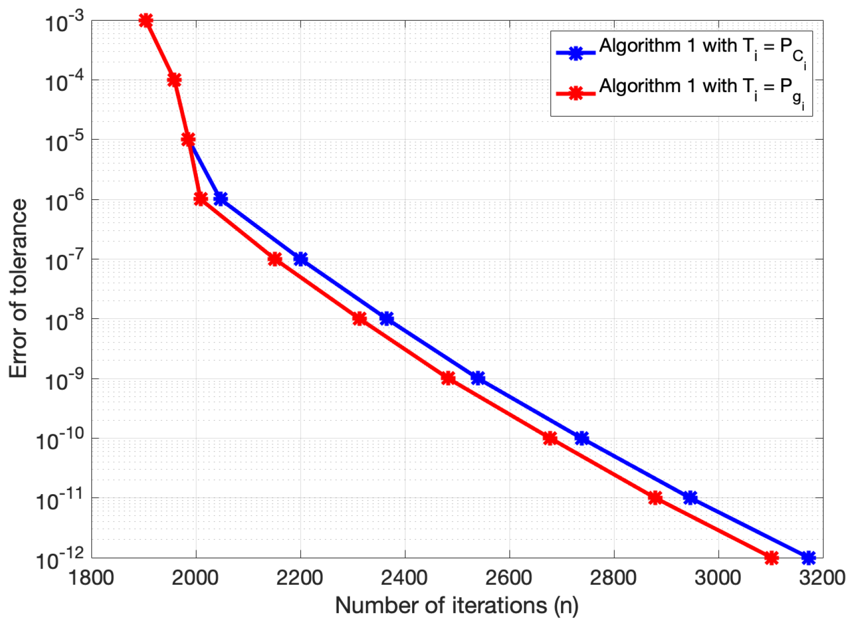
Finally, we present the comparison of the use of the subgradient projection and the metric projection for various optimality tolerances $\epsilon$. We set $n=500$ and $m=50$ and choose the corresponding parameters in the same manner as above, the average numbers of iterations with respect to the optimality tolerances are presented in Figure 1.

Figure 1. Comparison between the using of the subgradient projection $T_i=P_{g_i}$ and the metric projection $T_i=P_{C_i}$ with different errors of tolerance.

The plots in Figure 1 show that using the subgradient projection is more efficient than the metric projection for all the optimality tolerances. This emphasizes the superiority of using the subgradient projection when performing Algorithm 1.

5. Conclusions

In this work, we consider the solving of the bilevel equilibrium problem governed by a strongly monotone bifunction over the intersection of fixed-point sets of cutter operators. We associated with it the so-called subgradient-type extrapolation cyclic method. We present that the generated sequence generated by the proposed method converges to the unique solution to the problem. Our numerical experiment showed that using appropriate operators can yield a better convergence behavior to the proposed method.

It can be seen that the proposed subgradient-type extrapolation cyclic method (Algorithm 1) allows us to compute the operator $T_i,i=1,\dots ,m$, sequentially. The main advantage of our method is that the computing machine is not necessary to store information while computing. Notwithstanding, the nature of the cyclic method, it is well-known that to compute $S_i,$, the cyclic method needs to have the estimate $S_{i-1}$ in hand. This means that there has a waiting process while performing the method. In this case, one may consider the simultaneous extrapolation method [25] when dealing with the common fixed-point constrained of BEP.