Pattern Formation and Aggregation in Ensembles of Solitons in Quasi One-Dimensional Electronic Systems

Abstract

Broken symmetries of quasi one-dimensional electronic systems give rise to microscopic solitons taking roles of carriers of the charge or spin. The double degeneracy gives rise to solitons as kinks of the scalar order parameter A; the continuous degeneracy for the complex order parameter $Aexp\left(i\theta \right)$ gives rise to phase vortices, amplitudes solitons, and their combinations. These degrees of freedom can be controlled or accessed independently via either the spin polarization or the charge doping. The long-range ordering in dimensions above one imposes super-long-range confinement forces upon the solitons, leading to a sequence of phase transitions in their ensembles. The higher-temperature T transition enforces the confinement of solitons into topologically bound complexes: pairs of kinks or the amplitude solitons dressed by exotic half-integer vortices. At a second lower T transition, the solitons aggregate into rods of bi-kinks or into walls of amplitude solitons terminated by rings of half-integer vortices. With lowering T, the walls multiply, passing sequentially across the sample. Here, we summarize results of a numerical modeling for different symmetries, for charged and neutral soliton, in two and three dimensions. The efficient Monte Carlo algorithm, preserving the number of solitons, was employed which substantially facilitates the calculations, allowing to extend them to the three-dimensional case and to include the long-range Coulomb interactions.

1. Introduction: Confinement and Phase Transitions in Ensembles of Solitons

Strongly correlated electronic systems are prone to spontaneous symmetry breaking which brings about a manifold of degenerate ground states. Such degeneracy makes possible the existence of topologically non-trivial configurations connecting different states (see [1] for a latest review). These include, for example, domain walls and stripes, dislocations and vortex lines, as well as their complex aggregates. In two- and three-dimensional systems such objects are still macroscopic. However, in one-dimensional (1D) systems they become truly microscopic objects carrying energy, charge, and other quantum numbers of a single-electron scale. It appears, frequently, that such microscopic quasi-particles, called solitons, become the lowest energy excitations and take over the role of conventional electrons, e.g., in transport or optical properties (see [2,3] for short reviews). Since the solitons possess such non-zero quantum numbers as charge or spin, their stable ensembles can be controllably created and/or observed by the usual means, such as scanning tunneling microscopy. Such collective systems typically experience a sequence of phase transitions, accompanied by the formation of structures at an increasing scale: from individual solitons, via their microscopic complexes and growing aggregates to macroscopic domain walls and stripes.

The popular notion of “topological solitons” is a shortening for “topologically nontrivial solitons” which still needs precision such as “topologically stable …” or “topologically protected …”. The “topological stability” is based on conservation of “topological charges” and the related “irreducibility of trajectories” connecting different states of a systems, see reviews [4,5]. Following only the minimal feature of a spanning trajectory, with no respect to its reducibility, we shall imply a broader while less precise definition of a “topologically nontrivial soliton” as a local configuration exploring a manifold of degenerate ground state connecting different equivalent ones. The configurations may not be topologically stable, thus allowing for their transmutations with trivial electronic excitations. Such solitons appear or are preserved because they are energetically preferable and/or because the total electric charge or spin, which these solitons carry on, are monitored externally.

A major puzzle, as well as the inspiration, is that experimentally the solitons were observed or looked for within the low-temperature phases with a long-range order. The commonly unattended obstacle is the effect of the confinement of solitons (see [2] and refs. therein). Commuting between degenerate minima at only one chain would lead to a loss of the interchain ordering energy proportional to $\left|x\right|$—the distance along the chain till the next soliton or a boundary. This energy dominates at long distances even if it can be unimportant locally for a weak interchain interaction.

These interactions can appear already in some specific $1D$ systems where the ground state degeneracy is not exact, so the soliton connects the true and the false vacuums losing the confinement energy. The effect of confinement is omnipresent at higher dimensions where the interchain interactions, which are responsible for establishing the long-range $2D$ or $3D$ ordering, lift the degeneracy locally. In cases of discrete symmetries (when solitons are the amplitude kinks as in the $Z_2$ case of the dimerization) the solitons are bound in topologically trivial pairs with an option for a subsequent phase transition to form cross-sample domain walls [6,7,8]. Much richer are the cases of continuous symmetries: the phase degeneracy in superconductors and incommensurate charge density waves (ICDW), the directional degeneracy in spin-isotropic antiferromagnets, and both phase and spin degeneracy in spin density waves (SDW). Here, the gapless mode can cure the interruption from the amplitude kink which allows for individual solitons to enter the low-temperature phases with long-range ordered states. The solitons adapt by forming topologically bound combined complexes with half-integer vortices of gapless modes: $\pi$-rotons [2,3]. For cases of repulsing and attracting electronic interactions correspondingly, that results in spin- or charge-roton configurations with charge- or spin-amplitude solitons localized in the core. Beyond the quasi-1D electronic systems, the interference of different types of topological defects has been noticed already in the theory of superfluid phases in surface layers of ${\mathrm{He}}_3$ [9,10] and recently in doped antiferromagnets [11].

In this short review, we shall summarize and update our recent, largely numerical, studies on statistical ensembles of solitons [12,13], see also [14]. We refer to these publications for a broad review of experimental motivation and for a wider citations of the theoretical literature, while here we shall be concerned with only major theoretical aspects. Section 2 will be devoted to solitons in systems with a discrete double degeneracy. Separate sections will describe cases of neutral and charged solitons, modeling in $D=2$ and $D=3$ dimensions, slow a cooling and a quench. Section 3 will be devoted to a richer system with a combined amplitude-phase degeneracy, with numerical results shown for $D=2$, prone to combined topological defects with half-integer vorticity. Section 4 will be devoted to discussions and conclusions.

2. Discrete Symmetry: Solitons in Doubly-Degenerate Systems

In this chapter we shall address the case of a discrete symmetry breaking, particularly the double degeneracy, which is a very common phenomenon of a dimerization of bonds (the family of Peierls-like transitions) and/or of sites (the family of transitions with charge ordering or disproportionation). The alternation of spontaneously different sites or bonds allows for disruptive defects which passing changes the sign of the order parameter $A\to -A$, hence a soliton with a nickname the “kink”. In relevant electronic systems the soliton forms a potential wall possessing the bound “mid-gap” state which is allowed to capture one or two electrons, giving rise to oppositely charged spinless and/or neutral (or sometimes also charged) spin-carrying solitons. In a 1D-system or at high-temperature (T) disordered phase at a higher dimension (D), the randomly distributed solitons break the long range correlation at a length of the order of a mean distance among the kinks. Commonly, the on-chain interactions among solitons are short range (falling exponentially) repulsive. There are special cases of a highly degenerate energy landscape with a coalescence of different ground states, when the interaction among solitons becomes long ranged, decaying only as power laws (see [15] and refs. therein). Still, this is a weak effect in comparison with non-decaying confinement forces produced by interchain interactions which we shall study below.

At $D>1$ with lowering T, the interchain correlation of kinks enters the game drastically. Figure 1a,b shows that the energy of interchain interactions increases with growing separation between two solitons both on the same chain or on neighboring chains. Hence, there are two tendencies: either towards the formation of intra-chain bound pairs of solitons (which we shall call bi-solitons or bi-kinks), or towards inter-chain aggregation of solitons into the kink walls. As a result of these competing trends, the system goes through two phase transitions: the intra-chain pairing of solitons at a higher $T=T_1$, see Figure 1c,d, and the inter-chain aggregation of pairs at a lower $T=T_2$, see Figure 1e,f. The upper $T_1$ is the transition temperature where the long range is established for the order parameter: $⟨A⟩\ne 0$ at $T<T_1$, while for solitons it is the onset of their pairwise confinement. For a three-dimensional system, $T_2$ is a specific phase transition point; below this temperature there appear domain wall planes, which pass through the entire cross section of the sample. For a two-dimensional system, this is not a phase transition, but rather a crossover: with lowering the temperature below $T_2$, finite bi-solitonic rods (pieces of paired domain walls) gradually grow in the transverse direction. For finite systems, as in our numerical simulations, there exists a sample-dependent temperature $T_F$, at which the first wall crosses the entire sample even in a two-dimensional system.

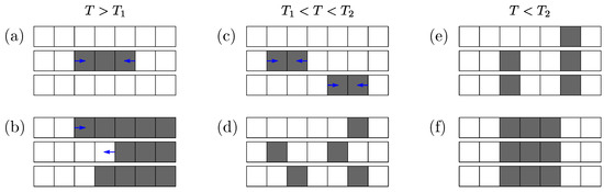
Figure 1. Schemes of interactions and aggregations of solitons for a three-chain fragment. White and gray squares correspond to different signs of the order parameter, their boundaries in the direction of chains correspond to solitons; blue arrows show forces acting upon them. At $T>T_1$, the kinks exist as separate objects, but they already experience a long-range attraction that links them into pairs on the same chain (a) or into walls across the chains (b). At $T_1>T>T_2$, the solitons are bound forming an ensemble of bisolitons (c). The lengths of bisolitons are large and fluctuate at $T_1>T>J_{\perp }$ (c). The bisolitonic pairs are tight at $J_{\perp }>T>T_2$ (d). At $T<T_2$, the bisolitons aggregate into growing bisolitonic walls (e) and then, reaching the sample boundaries, they split into isolated walls of kinks (f).

This qualitative picture is supported by an exact solution available for a $2D$ system of neutral solitons with some qualitative extensions to the $3D$ case [6]. The case of electrically charged solitons has been addressed in [7,8], but the numerical studies [7] suffered with a restrictive constraint: the bi-kink pairs were not allowed to jump between the chains. Following the approach of [12], here we shall present the results of unrestricted numerical modeling performed for the challenging case of a $3D$ system, both for neutral and charged ensembles of solitons.

2.1. Mapping to the Constrained Ising Model

The doubly-degenerate system can be mapped [6] upon the Ising model for spin variables $S_{n,\alpha }=\pm 1$ defined upon the discretized (with a distance $a_{\left|\right|}$) sites n of chains $\alpha$. The local density of kinks ${\rho }_{n,\alpha }$ can be expressed as

$${\rho }_{n,\alpha }=(1-S_{n,\alpha }{S}_{n+1,\alpha })/2,⟨{\rho }_{n,\alpha }⟩=\nu =N/V,$$

where $\nu$ is the mean concentration of solitons per site, N is their total number, $V=L\times H^{D-1}$ is the system volume with $L,H$ being the sizes along and transverse the chains. The mean density $\nu$ of solitons can be controlled by their chemical potential $\mu$, then the Gibbs energy ${\tilde{H}}_0$ for the grand canonical ensemble of solitons becomes

$${\tilde{H}}_0=H_0+(E_s-\mu )N=-J_{\perp }\sum _{⟨\alpha ,\beta ⟩n}{S}_{n,\alpha }{S}_{n,\beta }-J_{\left|\right|}\sum _{\alpha ,n}(S_{n,\alpha }{S}_{n+1,\alpha }-1),$$

(1)

where the transverse spin-coupling constant $J_{\perp }$ comes from the given energy of interchain interactions while the longitudinal one $J_{\left|\right|}=(\mu -E_s)/2$, where $E_s$ is the energy paid to create the defect, is variable together with $\mu$.

For electrically charged solitons we must add also [7,8] the Coulomb energy $H_C$:

$$\tilde{H}={\tilde{H}}_0+H_C,H_C=\frac{e^2}{2ϵ}\sum _{n,m;\alpha ,\beta }\frac{({\rho }_{n,\alpha }-\nu )({\rho }_{m,\beta }-\nu )}{|{\mathbf{r}}_{n,\alpha }-{\mathbf{r}}_{m,\beta }|},$$

(2)

where e is the electron charge and $ϵ$ is the dielectric constant.

In the resulting anisotropic Ising model (1), only the interchain coupling constant $J_{\perp }$ has a physical nature and remains fixed, while the intrachain coupling constant $J_{\left|\right|}$ is determined by the chemical potential of solitons. Controlling $\mu$, a grand canonical ensemble of solitons in D dimensions can be mapped to the D-dimensional Ising model, whereas the canonical ensemble can be mapped to a stack of non-interacting $(D-1)$-dimensional Ising models with a global constraint $⟨{\rho }_{n,\alpha }⟩=\nu$. The latter case of controlling the concentration $\nu$ corresponds to our physical situation of interest, where the source of the most interesting behavior comes from inverting the self-consistency condition $\nu (\mu ,T)$ to $\mu (\nu ,T)$, which means moving along a special line in the parameter space of the Ising model {$J_{\left|\right|},J_{{}_{\perp }},T$}. Alternatively, it is possible to construct a numerical procedure [12], which allows us to implement the constraint explicitly by preserving the total number of solitons. In this case, we work directly with the canonical ensemble and taking advantage of working with $(D-1)$-dimensional systems in which only physical interchain interaction is present.

2.2. Summary for the Effective Ising Model for a Neutral System

Recall the picture of equilibrium states for a neutral system (Figure 1). As the temperature decreases at a given concentration $\nu$ of solitons, the system goes through a sequence of two phase transitions (at $T=T_1$, $T_2$) and a crossover between them (at $T\approx J_{\perp }$). These temperatures are governed by three energy scales: $J_{\perp }$ as the local energy of interchain ordering, larger $T_1\propto J_{\perp }/\nu$ as the nonlocal energy of soliton confinement, and the smaller $T_2\propto J_{\perp }/ln(1/\nu )$ as characteristic energy of the transverse aggregation of solitons.

I. $T_1\propto J_{\perp }/\nu$. For the Ising order parameter $⟨S⟩$, this is simply the temperature $T_1=T_c$ of the second-order phase transition to a state with its non-zero mean at $T<T_c$. However, for an ensemble of solitons, this is a confinement–deconfinement phase transition. It occurs when the temperature drops below the average interchain interaction $Fl$, where $l=a_{\left|\right|}/\nu$ is the mean distance between solitons. At $T<T_1$, individual solitons become confined into loose intra-chain pairs; at the lower $T\sim J_{\perp }$, the pairs evolve into tightly bound “bisolitons”.

II. $T_2\propto J_{\perp }/ln(1/\nu )<J_{\perp }$. This is the temperature of solitons’ transverse aggregation, when the first domain walls crossing the entire sample emerge. Since, at $T=T_2$, we have $J_{\left|\right|}\left(T_2\right)=0$, the effective dimensionality of the system D is reduced by 1. With aggregation of bisolitons into the domain walls, the confinement energy is gained due to the proper ordering between neighboring chains. With that, the entropy is lost, and this balance sets the temperature $T_2$.

The bisolitonic pairs still coexist with walls below $T_2$, but as the temperature decreases further, the pairs disappear, giving material for building new domain walls. The basic intuition for ordered systems (e.g., Ising model) tells us that at low T the system remains in a simple form of a single ordered domain, diluted by rare spin-flips—tightly-bound bisolitons with an energy of $2N{J}_{\perp }$. However, with our constraints, the picture is different. The self-consistent concentration of bi-kinks is

$${\nu }_{bk}\approx exp\left(-\frac{4J_{\left|\right|}+2N{J}_{\perp }}{T}\right),$$

(3)

where N is the number of nearest chains. Since the concentration is fixed at ${\nu }_{bk}=\nu /2$, then the decrease in temperature must be compensated by the decrease in $J_{\left|\right|}$, which nevertheless must remain non-negative $J_{\left|\right|}\ge 0$. Hence, a new soliton storage reservoir must be opened, with $J_{\left|\right|}$ remaining equal to zero when T decreases below $T_2\left(\nu \right)$ such that $\nu =2exp(-2N{J}_{\perp }/T_2)$, i.e.,

$$T_2\approx \frac{2N{J}_{\perp }}{ln(2/\nu )}.$$

(4)

This reservoir is a system of stripes (lines in $2D$ or planes in $3D$) that cross the entire sample, dividing it into domains of alternating magnetization. In three-dimensional systems, below $T_2$ the transverse layers do not interact and $J_{\left|\right|}$ stays at zero value, hence $T_2$ must be indeed a sharp phase transition. In two-dimensional systems, $T_2$ is only a crossover for nucleation of growing rods of finite length. In $2D$, only for a finite sample of a width H, the rods grow through its entire cross-section at a temperature $T_F\approx 4J_{\perp }/ln(H/2\nu )$.

2.3. Numerical Approach for Ensembles of Amplitude Solitons

In this section, we review our numerical Monte Carlo (MC) results for $2D$ and $3D$ cases of neutral and charged solitons [12]. As we pointed out above, in the numerical simulations it is more efficient to preserve a fixed number of solitons, while for analytical calculations it is more favorable to use self-consistent $J_{\left|\right|}(T,\nu )$ approach, which was more convenient for the qualitative analysis and the access to exact solutions in $D=2$ [6]. We will work in the canonical ensemble representation, keeping fixed only the total number of solitons, while allowing to exchange them between the chains (in contrast to the more restrictive condition of fixing their number at the individual chains used in ref. [7]). For charged solitons, it is also necessary to consider the long-range Coulomb interactions, which is always a difficult task, especially in our case of pattern-prone system, where locally non-compensated charges appear at growing scales.

2.3.1. Neutral Solitons

We start with the basic case of the ensemble of neutral solitons. Figure 2 presents typical patterns of formation and reproduction of domain walls and discs (paired walls). At higher temperatures ($T=2.1J_{\perp }>T_2$, Figure 2a) the system is in an ordered state diluted by a gas of bisolitons. With the formation of the first pair of domain walls (at $T=2.0J_{\perp }\approx T_2$, Figure 2b), the concentration of non-condensed solitons drops, further decreasing gradually to cure the voids in already existing bisolitonic walls which then diverge and form two solitonic ones, giving rise to a domain of inverted spins between them. Then, the concentration of noncondensed solitons drops abruptly again with the formation of the another bisolitonic wall ($T=1.6J_{\perp }<T_2$, Figure 2c).

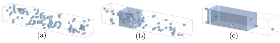
Figure 2. Formation of domain walls in a system of neutral solitons with the size $50\times 8\times 8$ and the solitons’ concentration $\nu =0.08$. (a) $T=2.1J_{\perp }$—no walls; (b) $T=2.0J_{\perp }$—two soliton walls; (c) $T=1.6J_{\perp }$—four soliton walls.

Interestingly, the second bisolitonic wall emerges in the vicinity of the first soliton wall. Presumably, this is because the motion of bisolitons intending to build the second wall is forbidden in the direction of the existing wall, which halves the probability of their escape, and thus facilitates the aggregation of the incipient second pair of walls.

2.3.2. Charged Solitons

Next, we address the case of electrically charged solions, focusing on the most interesting regime of intermediate values $J_{\perp }/H^2\ll V_C\ll J_{\perp }$ of the Coulomb parameter $V_C=e^2/ϵa_{\perp }$ ($a_{\perp }$ is the interchain distance). Now, $V_C$ is locally sufficiently weak, that it does not prevent the binding of kinks into bi-kinks; but even more than that—it does not prevent the initial aggregation of bi-kinks at neighboring chains into small disks. However, CI plays an important role for the large-scale structures, e.g., for large disks and domain walls, because for $V_C\gg J_{\perp }/H^2$ the formation of a wall planes is energetically unfavorable.

Thus, in contrast to the neutral solitons and weak CI cases, we do not observe a sharp transition of wall formation for intermediate values of the Coulomb parameter. We still observe finite bi-walls, possessing now the void defects. As the temperature approaches zero, these defects can merge, cutting the wall along one of the transverse directions (Figure 3a). At higher values of the Coulomb parameter, no plane walls are formed at all, but filamentous stripes emerge instead, which are infinite along one of the transverse directions and finite along the other one (Figure 3b).

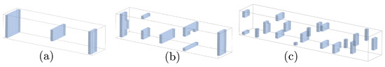
Figure 3. Disintegration of domain walls as the CI increases. Modeling for a system with a size $50\times 8\times 8$ at $\nu =0.08$ and $T=0.1J_{\perp }$ for different values of the Coulomb parameter: (a) $V_C=0.02J_{\perp }$, (b) $V_C=0.1J_{\perp }$, (c) $V_C=0.3J_{\perp }$.

Formation of lines rather than planes demonstrates the extreme sensitivity of CIs to the pattern geometry. A charged plane wall would create a constant electric field $E=4\pi e/\left(ϵa_{\perp }^2\right)$ in the chains’ x direction, whose repulsive force $eE$ would oppose directly the attractive confinement force $F=2Z{J}_{\perp }$ overpassing it at the intermediate CI, hence no stable planes could exist. However, forming the stripes (in one transverse y direction) at the expense of the part of the confinement energy (lost in the other transverse direction z), the system generates a decreasing electric field $E\propto 1/\sqrt{x^2+z^2}$ which falls below the confinement force at sufficiently large distances, hence preserving the partial aggregation. We expect that for an infinite system these structures will further disintegrate into finite pieces. For an even higher value of the Coulomb parameter, the formation of stripes becomes also energetically unfavorable even for a finite system, and we observe only disks of bi-kinks (Figure 3c). For an even stronger Coulomb interaction $V_C\gtrsim J_{\perp }$, the transverse disks shrink to the minimum size of one bi-kink which form a Wigner “liquid”, then the crystal, and finally a crystal of solitons. The latter state is the universal limit of any system of dilute point charges.

3. Pattern Formation in Ensembles of Phase-Amplitude Solitons for a Complex Order Parameter

In this chapter, we construct and study the coarse-grained model of XY–Ising type, which describes the local and the long-range orderings under the created and then monitored mean concentration of solitons. We shall demonstrate an evolution of ensembles of solitons via a sequence of phase transitions or crossovers. At $T<T_1$ the interchain correlations settle in, and dilute amplitude solitons are dressed by half-integer vortex rings (vortex-antivortex (VA) pairs in $D=2$). Upon further cooling towards a lower $T_2$, the solitons start to aggregate in the transverse direction forming domain walls terminated by the half-VA pairs. The terminating half-vortices at neighboring walls interact by pseudo-Coulomb forces. Attraction and subsequent annihilation of vortices of opposite signs belonging to neighboring walls favors the gluing of walls, either sequentially, elongating their lengths, or parallelly forming bisolitonic rods. Both scenarios will be visualized in our modeling. At $T<T_2$ in $D=3$, or at a size-dependent temperature $T_F\sim T_2$ at $D=2$, the solitonic walls grow across the whole sample and finally the regular “stripe phase” sets in.

3.1. Solitons in Quasi-1D Systems with Combined Amplitude and Phase Degeneracies

Most important cases of degenerate ground states in electronic systems (superconductivity, incommensurate CDWs) invoke a complex order parameter $\mathcal{O}=Aexp\left(i\theta \right)$. Almost commonly, the amplitude A is assumed to be positive $A>0$ being associated with a “superfluid” or “collective” densities $A={\rho }_s,{\rho }_c$ known also as the “phase rigidity”. With respect to the flexible phase $\theta$ which variations give rise to observable collective currents, sound waves and vortices, the amplitude is considered to be only weakly perturbed, except for its enforced vanishing at cores of phase vortices. However, the microscopic insight at quasi-1D electronic systems (see [2,3]) shows that actually A is an independent local degree of freedom which should not be positively defined and, moreover, the alternations of its sign are related to monitored quantum numbers.

Recall briefly some most basic facts on solitons in spin-singlet ground states of electronic systems: ICDWs and quasi-1D superconductors (see refs. in [2,3]). The ICDW is a weak crystal $Acos(2K_{f}x+\theta )$ of the electronic density and atomic displacements with the order parameter is ${\mathcal{O}}_{ICDW}=Aexp\left(i\theta \right)$. The singlet pair can be broken into spin $1/2$ components, but instead of expectedly liberated electron–hole pair at the gap rims $\pm \Delta$, there will be spin-carrying “amplitude solitons” (AS)—nodes of the order parameter distributed over the length $\xi \sim 1/\Delta$. The total energy of the soliton is $E_s\approx 2\Delta /3<\Delta$ making it energetically favorable with respect to the energy $\Delta$ of the undressed unpaired electron which now is trapped at the mid-gap state associated with the amplitude soliton. This electron brings the spin $1/2$, but its charge is compensated to zero by the local dilatation in the occupied manifold of singlet vacuum states. That makes the AS a CDW realization of the “spinon”, with a direct generalization to a superconductor [16] where the AS appears as the node line in the so called Fulde–Ferrel–Larkin–Ovchinnikov (FFLO) phase in spin-polarized superconductors (see [3] and refs. therein).

The amplitude soliton $A(x=-\infty )\Rightarrow -A(x=+\infty )$ performs the sign change of the order parameter $\mathcal{O}$ at an arbitrary phase $\theta =const$. As a non-trivial topological object (the order parameter ${\mathcal{O}}_{cdw}\left(x\right)=A\left(x\right)exp\left(i\theta \left(x\right)\right)$ does not map onto itself), the pure AS (with $\theta \left(x\right)=const$) is prohibited in $D>1$ environment. At higher space (or space-time for instantons) dimensions D, the requirement always appears that the order parameter is mapped onto itself. Even having a lower energy in comparison with the band electron, the purely amplitude soliton cannot be created dynamically already in the $D=1$ space dimension, and it is not allowed even stationary at $D>1$. The conflict is resolved recalling the combined symmetry: the amplitude kink $A\Rightarrow -A$ accompanied by the half-integer $\theta \Rightarrow \theta \pm \pi$ vortex of the phase rotation, for which the factor $exp\left(i\theta \right(x\left)\right)$ compensates for the amplitude sign change. The resulting kink–roton complex allows for several interpretations in applications to ICDW or superconductors: $2D$ view is a pair of $\pi$-vortices sharing the common core which accommodates one unpaired spin which stabilizes the state; $3D$ view is a ring of a half-integer vortex ring which center confines the spin; at any $D>1$ this is a nucleus of the melted FFLO phase in the spin-polarized superconductors or its CDW analogue, see [3]. In repulsive electronic systems, basically the SDW and the doped antiferromagnetic state, the situation is mirror symmetrical: the amplitude node carries the electronic charge $\pm e$ while the wings of half-integer vortices provide a distributed spin $1/2$, see [2,3].

3.2. The Effective Model and the Qualitative Phase Diagram

A discrete description of a quasi-1D system with both the amplitude A and the phase $\theta$ degrees of freedom can be based upon the energy functional

$$H=-C\sum _{r}cos({\theta }_r-{\theta }_{r+\widehat{x}})-J_{\perp }\sum _r{s}_r{s}_{r+\widehat{y}}cos({\theta }_r-{\theta }_{r+\widehat{y}})-J_{\left|\right|}\sum _r{s}_r{s}_{r+\widehat{x}}.$$

(5)

Here, the Ising variable $s_r=\pm 1$ corresponds to the normalized amplitude of the complex order parameter and the angle ${\theta }_r$ corresponds to its phase; r runs over sites of a lattice including the chains’ direction $\widehat{x}$ and the interchain vector $\widehat{y}$. The last term with $J_{\left|\right|}=(\mu -E_s)/2$ fixes the chemical potential $\mu$ of amplitude solitons, similarly to the $Z_2$ symmetry case of the previous chapter.

The Hamiltonian (5) describes two interfering subsystems: an Ising model which interchain coupling is modulated by phase distortions, and the XY model which interchain rigidity is interrupted by defects of the spin ordering. It is conceptually close to the Korshunov’s $2\theta$ model [9,10] and the coupled XY–Ising model [17,18]. The Hamiltonian (5) is invariant under a semi-local gauge transformation of simultaneous flipping of all Ising spins and all XY vectors within any given chain y independently: $s_r\to -s_r,{\theta }_r\to {\theta }_r+\pi$. That implies vanishing of macroscopical averages and the interchain correlations of Ising and XY fields separately: $⟨s_r⟩=0$, $⟨exp\left(i{\theta }_r\right)⟩=0$. Still, a combined variable—the physical order parameter ${\Delta }_r=s_r{e}^{i{\theta }_r}$—possesses the correlation functions and can acquire a nontrivial average.

Similarly to the case of the $Z_2$ symmetry, we expect two successive phase transitions at $T_1$ and $T_2$. The long range ordering is established at $T_1$, so that only at $T>T_1$ the amplitude solitons exist in their pure form at uncorrelated chains. For the $3D$ system, the upper transition temperature $T_1$ of the $Z_2$ case is generalized as a critical temperature $T_c$ which character will change along the line $T_c\left(\nu \right)$, see Figure 4. The line can be determined within the mean-field approximation with the expansion in powers of the order parameter $\eta$:

$$⟨s_{r}cos\left({\theta }_r\right)⟩=\eta ,\mathrm{while}⟨s_r⟩=0,⟨cos\left({\theta }_r\right)⟩=0.$$

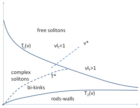
Figure 4. Phase diagram of a $3D$ system in temperature vs solitons’ concentration coordinates in the regime of weak interchain coupling. Notations are explained in the text.

At $T>T_1$, $\eta =0$; the interchain interactions can be neglected so that only intra-chain correlations are present:

$$⟨s_{00}{s}_{0x}cos\left({\theta }_{00}\right)cos\left({\theta }_{0x}\right)⟩\Rightarrow ⟨s_{00}{s}_{0x}⟩⟨cos\left({\theta }_{00}\right)cos\left({\theta }_{0x}\right)⟩=exp(-\nu |x|-|x|/l_T),l_T\sim C/T,$$

where $l_T$ is the phase correlation length in the 1D regime. The mean-field Hamiltonian

$$H=-C\sum _{r}cos({\theta }_r-{\theta }_{r+\widehat{x}})-J_{\perp }\eta \sum _r{s}_{r}cos\left({\theta }_r\right)-J_{\left|\right|}\sum _r{s}_r{s}_{r+\widehat{x}}$$

gives rise to the self-consistent equation which, in the first order in $\eta$, reads

$$\begin{array}{cc}\hfill \eta & =\eta N{J}_{\perp }\sum _x⟨s_{00}{s}_{0x}cos\left({\theta }_{00}\right)cos\left({\theta }_{0x}\right)⟩,\eta \ne 0\mathrm{if}:\hfill \\ \hfill 1& =N{J}_{\perp }/T_c\sum _{x}exp(-\nu |x|-|x|/l_T)=\frac{2N{J}_{\perp }/T_c}{\nu +T_c/C}\hfill \end{array}$$

(6)

where N is the number of nearest interacting chains. Equation (6) gives the dependence $T_c\left(\nu \right)$ via the equation $2N{J}_{\perp }/T_c-T_c/C=\nu$. There are two regimes:

$$\begin{array}{cc}\hfill T_c& \approx N{J}_{\perp }/\nu \mathrm{at}\nu >{\nu }^{\ast }=T_c/C\approx \sqrt{2N{J}_{\perp }/C}\hfill \\ \hfill T_c& \approx \sqrt{N{J}_{\perp }C}\mathrm{at}\nu <{\nu }^{\ast },max\left(T_c\right)=T_{c0}=\sqrt{2N{J}_{\perp }C}\mathrm{at}\nu =0\hfill \end{array}$$

(7)

with a crossover at $\nu ={\nu }^{\ast }$. The first line in Equation (7) implies a weak interchain coupling: $J_{\perp }\ll C$ when ${\nu }^{\ast }\ll 1$; otherwise, for a strong coupling $J_{\perp }\gg C$, only the regime of the second line takes place with a nearly constant $T_c\left(\nu \right)$. At $\nu >{\nu }^{\ast }$ the distance $1/\nu$ among solitons is shorter than the phase correlation length $l_T$, then the phase transition follows the $Z_2$ case scenario of pairwise binding of solitons; $T_c$ generalizes the $T_1$ transition temperature. At $\nu <{\nu }^{\ast }$ (hence for any allowed $\nu <1$ if ${\nu }^{\ast }>1$) the solitons are rare over the phase correlation length $l_T$ and the phase transition follows the XY regime of the phase ordering while isolated solitons are dressed, at $T<T_c$, by half-integer vortex rings.

Below $T_c$, there is a competition between the two forms of adaptation of solitons to the confinement. Because of the exchange of constituting particles, the chemical potentials are equilibrated. Then, the concentrations of bi-kinks and solitonic complexes are given as

$${\nu }_{bk}=exp\left(\beta (2\mu -2E_s-2N{J}_{\perp })\right),{\nu }_s=exp\left(\beta (\mu -E_s-E_V)\right),2{\nu }_{bk}+{\nu }_s=\nu ,$$

where $N{J}_{\perp }$ is the interchain energy paid over the bi-kink, $E_V\mathsf{\propto }{T}_{c0}$ is the energy of the vorticity accompanying the soliton. We can easily conclude that the total concentration is dominated by solitons, $\nu \approx {\nu }_s$, if: (a) at any $\nu ,T$ in the strong coupling case when $N{J}_{\perp }\gg E_V$ and (b) in the weak coupling case $N{J}_{\perp }\ll E_V$ at sufficiently high $T>T^{\ast }=2(E_V-N{J}_{\perp })/ln(1/\nu )$. Neglecting the minor ${\nu }_{bk}$, the condition $\mu -E_s=0$ determines the phase transition of aggregation of solitons into the domain walls as $\nu =exp\left(-E_V/T_2\right)$, $T_2=E_V/ln(1/\nu )$. This estimation works indeed for the strong coupling case. For the weak coupling, such a defined temperature $T_2$ is below the crossover, $T_2<T^{\ast }$, where actually the concentration is dominated by the bi-kinks. Hence, with cooling below $T_c$, the ensemble of combined solitons evolves to the ensemble of bi-kinks while passing through the crossover $T^{\ast }$. Then, the bisolitonic mechanism of aggregation into double-wall rods takes place below the temperature estimated as $T_2^{\prime }=N{J}_{\perp }/ln(1/\nu )$, analogously to the $Z_2$ case.

In the dimension $D=2$, the above estimations of $T^{\ast },T_2$ for the bi-kinks regime are valid except for the fact that $T_2^{\prime }$ becomes a crossover where the rods start to grow, rather than a sharp transition. Still, the solitonic mechanism of the strong coupling keeps the sharp transition. This nontrivial difference comes from long range pseudo-Coulomb interactions of half-integer vortices terminating a finite segment of aggregated solitons. We can explain that by extending simple arguments which have been proved for the case of the discrete symmetry by comparison with the exact solution available at $D=2$ [6]. In the next section we shall illustrate them by means of the numerical modeling.

Consider a thermodynamically equilibrium system of transverse segments of solitonic walls of variable lengths l. Because of exchange of solitons among the rods, their chemical potentials are $\mu \left(l\right)=\mu l$. In $D=2$, their energies $E\left(l\right)$ can be estimated as:

$$E\left(l\right)=E_{s}l+2E_c+\frac{1}{2}\pi E_{V}lnl.$$

(8)

Here, $E_s$ is the core energy of the amplitude soliton; $2E_c\sim J_{\perp }$ is the local energy of termination points and the last term is the pseudo-Coulomb interaction between terminating half-integer vortices. The distribution of walls over their lengths $n\left(l\right)=exp\left(\left(\mu \right(l)-E(l\left)\right)/T\right)$ yields the total concentration of solitons as

$$\nu =\sum _{l=1}^{\infty }ln\left(l\right)=exp\left(-\frac{2E_c}{T}\right)\sum _{l=1}^{\infty }{l}^{1-\alpha }{e}^{-ml},m=\frac{(E_s-\mu )}{T}\ge 0,\alpha =\frac{\pi E_V}{2T}.$$

(9)

Recall the situation of the $Z_2$ case, where the expression (8) holds with $E_V=0$, hence $\alpha =0$ in (9). As $T\to 0$, the factor $exp(-2E_c/T)\to 0$, so to keep $\nu$ fixed, the sum in (9) needs to diverge at $m\to 0$ which would happen at $\alpha <2$. That holds indeed for the $Z_2$ case with $\alpha =0$, then $\nu \mathsf{\propto }exp\left(-2E_c/T\right)/m^2$ which yields the characteristic rod length growing with T as

$$l\mathsf{\propto }\frac{1}{m}\mathsf{\propto }\nu exp\left(E_c/T\right).$$

For the system with the vorticity when $E_V\ne 0$, the $m\to 0$ divergence requires that $T>\pi E_V/4\simeq T_{c0}$. However, we are in the region well below $T_{c0}$ where $\alpha >2$, then the sum in (9) is bounded from above being convergent even at $m=0$. Therefore, the ensemble of finite wall segments cannot further accommodate all the solitons, with the rest of them being stored in a reservoir played by domain walls crossing the sample. The temperature of this condensation is given by Equation (9) at $m=0$ which yields $T_2\approx 2E_c/ln(1/\nu )$. Figure 4 shows the expected phase diagram of the system for the simpler case of the strong interchain coupling.

The $2D$ case is special because of a particular role of thermally activated vortices leading to a famous physics of the Berezinskii–Kosterlitz–Thouless (BKT) transition, see [19,20]. Here, our consideration is complicated by several factors. Phase fluctuations are essential even in the low T region, destroying the long range order while leaving the power law correlations. Vanishing of the order parameter at all temperatures leaves the mean field approximation for the upper transition at $T_c\left(\nu \right)$ (6) and (7) to be valid only locally. The thermally activated conventional integer vortices are abundant at high T, playing a leading role in the phase transition. These properties are well established for the pure XY model, which corresponds to our model in the limit $\nu =0$.

In the $2D$ case, the coexistence of integer and half-integer vortices and their relation to spin arrangements can be made explicit by the following procedure. Using the Villain approximation [21], we can find the “pseudo-Coulomb gas” representation of the statistical sum Z originated by the Hamiltonian (5):

$$\begin{array}{cc}\hfill Z& =\sum _{\left\{m_R\right\}}\sum _{\left\{s_r\right\}}exp\left(\pi \beta T_{c0}\sum _{R\ne R^{\prime }}(m_R+{\nu }_R)ln\frac{|\mathbf{R}-{\mathbf{R}}^{\prime }|}{a}(m_{R^{\prime }}+{\nu }_{R^{\prime }})\right.\hfill \end{array}$$

$$\begin{array}{cc}\hfill & \left.+({\pi }^2\beta T_{c0}/2)\sum _R{(m_R+{\nu }_R)}^2+\beta J_{\left|\right|}\sum _r{s}_r{s}_{r+\widehat{x}}\right)\hfill \end{array}$$

(10)

$$\begin{array}{cc}\hfill {\nu }_R& =\frac{1}{4}(s_{r+\widehat{x}}{s}_{r+\widehat{x}+\widehat{y}}-s_r{s}_{r+\widehat{y}})=\{0,\pm 1/2\}\hfill \end{array}$$

(11)

Here, the indices r and R run over sites of the original lattice and the dual one correspondingly; the summation goes over all integer values of $m_R$ and all configurations of spins $s_r=\pm 1$. The vortex “charge” (the vorticity) $m_R+{\nu }_R$ can acquire, unusually, a half-integer value; moreover, it becomes dependent on the local configuration of spins. Apart from the conventional long-range pseudo-Coulomb energy associated with all vortices, there is an additional local Ising term $\sim J_{\left|\right|}$. The anomalous contribution to the vorticity ${\nu }_R$, see Equation (11), at a site R emerges for particular configurations of spins $s_r$ in the surrounding placket r: with three spins up and one down, or vice versa, see Figure 5. Such a configuration appears only as a termination of a transverse line of kinks: $s_r{s}_{r+\widehat{x}}=-1$ (the orange lines in Figure 5a and Figure 6), leading to the linearly growing, as $\left|y\right|J_{\left|\right|}$, of the $\sim J_{\left|\right|}$ term in (10). Thus, the longitudinal spin-coupling term with $J_{\left|\right|}\ne 0$ leads to confinement of half-vortex pairs, situated at the ends of transverse solitonic walls, preventing formation of single half-vortices.

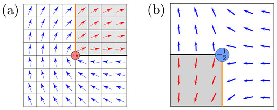
Figure 5. A half-vortex (a)—drawn schematically (after [13]), and a half-antivortex (b)-extracted from simulations of Figure 8. Here and in the following figures: arrows show XY degree of freedom, white/gray shading shows the Ising degree of freedom, the orange vertical (transverse to chains) thick line shows the array of amplitude solitons, the black horizontal (along the chains) thick line shows a string attached to a half-vortex—the line of transverse $\pi$-jumps in the phase $\theta$, the disks denote the cores of half-integer (anti)vortices. The orange line is a uniquely defined physical object: the $J_{\left|\right|}$ energy-costing spin mismatches. The black line is gauge dependent, lacking a physical singularity, with no energy cost.

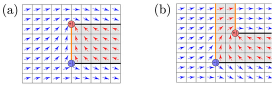
Figure 6. Half-integer vortex-antivortex pairs. (a) $T>T_2$, the pair structure is dominated by the linear confinement potential, solitonic walls (orange) are finite. (b) $T<T_2$, the pair structure is dominated by $2D$ Coulomb log-potential, solitonic walls grow to infinity. (After [13]).

At the special value $J_{\left|\right|}=0$, the Hamiltonian (10) gives rise to a BKT type physics of half-vortices with the associated BKT transition of unbinding of their pairs at $T=T_{BKT}^{half}=T_{BKT}/4$. The point $J_{\left|\right|}=0$ can be realized, in principle, experimentally by coupling to an electronic bath with an appropriate tuning of the voltage difference. For a closed system, the limit $J_{\left|\right|}\to 0$ is realized when the chemical potential of amplitude solitons is trapped at $E_s$, which happens below the temperature of the solitonic walls formation.

The opposite limit $\beta J_{\left|\right|}\to \infty$ means that $(\mu -E_s)/T\to -\infty$, i.e., the vanishing concentration of solitons. In this limit, the half-vortices are strongly confined by the energy-costly spin strings. The game is dominated by conventional thermally activated integer vortices which drive the conventional BKT type transition at $T=T_{BKT}\approx 0.9C$ between the high-temperature disordered phase and the low-temperature phase with algebraically decaying correlations.

For intermediate $J_{\left|\right|}$ we expect a crossover between regimes with domination of either integer or half-integer vortices.

The outlined phase diagram was confirmed via a numerical modeling by calculating macroscopic averages and their anomalies at phase transitions [12,13], and by displaying local pattern formations which examples we shall show below.

3.3. Pattern Formation from Numerical Simulations

In this section, we describe the pattern formation in relation to the phase diagram. First, recall the terminology. An amplitude soliton (or just a kink for brevity) is an interruption of the Ising order along the chains’ (x) direction, i.e., the soliton is present when $s_r{s}_{r+\widehat{x}}=-1$. A solitonic wall (or a line of kinks in $D=2$) is the aggregation of solitons transversely to the chains. (In the $3D$ case, the wall becomes a solitonic disk.) A domain wall appears when a solitonic wall grows across the whole transverse section of the sample. A bisoliton consists of two kinks at the minimal in-chain distance a between them; it is a reversed spin $s_r$ in the otherwise ordered part of the chain. A rod in $2D$ is an aggregation of bisolitons arranged transversally to the chains. Analogous configurations in $3D$ are called “bisolitonic disks”. When such discs grow transversially and reach the boundaries of the system, we obtain bisolitonic domain walls.

We model the cooling behavior of a system described by the Hamiltonian (5) using the Metropolis Monte Carlo method. The numerical algorithm preserves the number of amplitude solitons (so the term $J_{\left|\right|}{\sum }_r{s}_r{s}_{r+\widehat{x}}=const$) which substantially simplifies the analysis. There are no restrictions upon the phase degree of freedom ${\theta }_r$.

Figure 7 shows a configuration with four solitons which are dressed by the phase adjustments $\theta \to \theta +\pi$, restoring the interchain order. Here, we observe two neutral half-VA pairs (outer ones) and also two charged half-VV and half-AA pairs (inner ones). The presence of such configurations with combined phase-amplitude topological defects grows with the increasing $J_{\perp }$. Sharper versions of such combined defects can be also found in a great number in Figure 8.

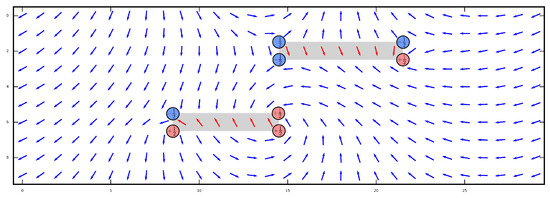
Figure 7. Configurations with four solitons for a system $10\times 30$ with $J_{\perp }=0.25C$, which was rapidly quenched down to $T\ll C$. Red and blue disks denote half-integer vortices and antivortices.

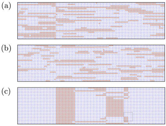
Figure 8. Configurations upon cooling for a system $25\times 100$ with a strong interchain coupling $J_{\perp }=4C$. (a) $T=0.31C$, (b) $T=0.30C$, and (c) $T=0.01C$. From (a) to (b) we see that the transverse rod of solitons grows across the whole sample towards formation of macroscopic domains in (c). The box in (c) shows the half-antivortex, presented in Figure 5.

3.3.1. Quasi-Equilibrium Cooling

We begin with the strong interchain coupling: $J_{\perp }=4C$. Cooling the system down starting from high temperatures, first we observe only short transverse solitonic walls (Figure 8a). At a temperature $T_2\approx 0.3C$ we observe a sudden change: one of the walls starts to grow until it reaches the borders of the sample (Figure 8b). With a further cooling, more solitonic walls appear (Figure 8c) until the material for their building—free solitons—is exhausted. All the domain walls are installed through the growth of solitonic walls.

For a weak interchain coupling $J_{\perp }=0.25C$, the walls formation is similar to the previously studied $Z_2$ case of the pure Ising model. The aggregation proceeds via proliferation of bisolitonic rods which do not need to be terminated by vortices (Figure 9).

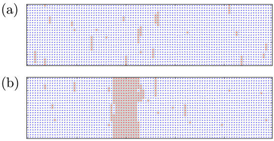
Figure 9. Configurations upon cooling for a weak interchain coupling $J_{\perp }=0.25C$. (a) $T=0.33C$, (b) $T=0.32C$.

3.3.2. Quench versus Cooling: Two Regimes of Aggregation

In this section, we simulate a sudden quench from high to low temperatures $T<T_2$. This scenario is relevant to modern experiments on phase transitions induced by optical or electrical pulses, particularly in CDWs and other electronic crystals, see the discussion and references in [14]. We shall demonstrate that even for the case of weak interchain coupling the setting of domain walls is dominated by the mechanism of aggregation of soliton–vortex complexes.

Figure 10 shows configuration of a system with a weak interchain coupling $J_{\perp }=C/4$ after a sudden quench from a high temperature $T>T_2$ to the low temperature $T=0.25C<T_2$. We observe the domain wall created by the solitonic mechanism, even if for the quasi-equilibrium slow cooling at the weak coupling the growth was dominated by the bisolitonic mechanism. When the solitonic wall initially starts to grow, half-vortices with opposite charges (vorticities) are created at its ends. These charges attract smaller solitonic rods via pseudo-Coulomb interaction mediated by the XY subsystem, promoting the further growth of the solitonic walls. The energy gain from merging of two walls is $\sim Clnl$, so the growth process is self-accelerating and for finite samples the solitonic walls can even grow across the whole sample. On the contrary, the growth of bisolitonic rods goes via attaching of new bisolitons at the ends—similar to the case of the $Z_2$ symmetry, which is a much slower random walk process. At the same time, longer solitonic rods become low-mobile, therefore their recombination to bisolitonic rods is kinetically suppressed.

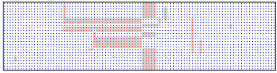
Figure 10. Configuration of the system after sudden quench from $T>T_2$ to $T=0.25C<T_2$ (for a system $25\times 100$ with $J_{\perp }=C/4$).

4. Conclusions

Solitons have returned to the agenda of studies of correlated electronic systems as their cooperative states can be created and studied in experiments on optical pumping and field effect doping. In this review, we have outlined results of the numerical and the qualitative analyses of phase transitions in ensembles of solitons. The numerical simulation of large-scale pattern formation in the full $3D$ system, including true Coulomb forces and for the combined discrete-continuous symmetry, was a challenging goal. The success came from using an efficient Monte Carlo algorithm which steps preserve the total number of solitons while allowing for their on-chain number variations. We have studied two of the most common cases:

I. The double degeneracy of the ground state which is found experimentally in electronic systems with a spontaneous dimerizations of bonds or charges. The solitons appear as kinks in the field of a scalar order parameter. In comparison with earlier studies [7], here we employed a more advanced numerical technique [12] which allowed us to model the pattern formation in D = 3, including the true Coulomb effects. Results of the modeling can be qualitatively summarized as following. The systems of solitons shows a sequence of phase transformations:

i.

The confinement transition at $T_1$, below which individual solitons are bound into on-chain pairs. It is followed by progressive aggregation of bisolitons into transverse disk-like or rod-like formations;

ii.

At a lower critical temperature $T_2$, the second phase transition (a crossover in $D=2$) occurs: the bisolitonic disks cross the entire sample and disintegrate into solitonic domain walls;

iii.

For electrically charged solitons, even locally small Coulomb interactions can nevertheless affect the $T_2$ transition where macroscopic patterns are created. A large scale structure, such as a domain wall, gives rise to a high long-range electric field withstanding the confinement forces. That erases the gain of the confinement energy reached by the wall formation, resulting in fragmenting macroscopic patterns which give rise to long-range electric field.

II. The combined degeneracy with respect to both the amplitude and the phase of the order parameter. The motivation of presented studies was to notice that most common types of symmetry breaking (superconductivity, spin density waves, antiferromagnetic Mott state, incommensurate charge density waves) in quasi-one-dimensional electronic systems possess a combined manifold of degenerate states. Beyond the standard continuous XY-type degeneracy with respect to the phase $\theta$ degree of freedom, there is also an Ising-type discrete degeneracy with respect to the sign of the amplitude A of the order parameter $Aexp\left(i\theta \right)$. These two degrees of freedom can be controlled or accessed independently via either the spin polarization or the charge doping. The degeneracies give rise to two coexisting types of topologically nontrivial configurations: phase vortices or amplitude kinks – the solitons. Being decoupled at the 1D level of isolated chains, at higher D the two degrees of freedom experience confinement which binds together kinks and half-integer vortices. These combined amplitude-phase solitons are the lowest-energy excitations of either spin or charge taking that role from conventional electrons. The case of the combined symmetry also shows a sequence of two phase transitions. At the higher $T_1$ the (quasi in D = 2) long-range order of the XY type sets in, leading to the confinement which dresses the kinks by half-integer vortices. At the lower $T_2$ the liquid of combined solitons starts to structure by aggregating the solitons into walls growing across the sample. That proceeds via either solitonic domain walls or bisolitonic rods. The growing solitonic walls are formed by transversely correlated amplitude kinks; termination points of walls of finite lengths must be accomplished by half-integer vortices. Attractions of vortices from different walls may force the walls to glue together forming a topologically trivial bisolitonic rod. For non-equilibrium processes, such as supercooling by a sudden quench, the solitonic-wall scenario can be strongly promoted because the growing solitonic wall has uncompensated half-vortex “charges” at the ends. They attract mobile smaller rods, while the slow process of gluing of low-mobile long solitonic walls into bisolitonic rods can be kinetically suppressed.

References

- Manton, N.; Sutcliffe, P. Topological Solitons; Cambridge University Press: Cambridge, UK, 2004. [Google Scholar]
- Brazovskii, S. New Routes to Solitons in Quasi One-Dimensional Conductors. Solid State Sci. 2008, 10, 1786–1789. [Google Scholar] [CrossRef] [Green Version]
- Brazovskii, S. Microscopic solitons in correlated electronic systems: Theory versus experiment. Advances in Theoretical Physics: Landau Memorial Conference. AIP Conf. Proc. 2009, 1134, 74. [Google Scholar]
- Mineev, V.P. Topologically Stable Dedects and Solitons in Ordered Media; Harwood Academic Publishers: Harwood, MD, USA, 1998. [Google Scholar]
- Mermin, N.D. The topological theory of defects in ordered media. Rev. Mod. Phys. 1979, 51, 591. [Google Scholar] [CrossRef]
- Bohr, T.; Brazovskii, S. Soliton statistics for a system of weakly bound chains: Mapping to the Ising model. J. Phys. C Solid State Phys. 1983, 16, 1189. [Google Scholar] [CrossRef]
- Teber, S.; Stojkovic, B.P.; Brazovskii, S.; Bishop, A.R. Statistics of charged solitons and formation of stripes. J. Phys. Condens. Matter 2001, 13, 4015. [Google Scholar] [CrossRef]
- Teber, S. Statistical properties of charged interfaces. J. Phys. Condens. Matter. 2002, 14, 7811. [Google Scholar] [CrossRef]
- Korshunov, S.E. Possible splitting of a phase transition in a 2D XY model. JETP Lett. 1985, 41, 263. [Google Scholar]
- Korshunov, S.E. Phase diagram of the modified XY model. J. Phys. C Solid State Phys. 1986, 19, 4427. [Google Scholar] [CrossRef]
- Grudst, F.; Pollet, L. Z2 parton phases in the mixed-dimensional t − Jz model. Phys. Rev. Lett. 2020, 125, 256401. [Google Scholar]
- Karpov, P.; Brazovskii, S. Phase transitions in ensembles of solitons induced by an optical pumping or a strong electric field. Phys. Rev. B 2016, 94, 125108. [Google Scholar] [CrossRef] [Green Version]
- Karpov, P.; Brazovskii, S. Phase transitions and pattern formation in ensembles of phase-amplitude solitons in quasi-one-dimensional electronic systems. Phys. Rev. E 2019, 99, 022114. [Google Scholar] [CrossRef] [PubMed] [Green Version]
- Karpov, P.; Brazovskii, S. Modeling of networks and globules of charged domain walls observed in pump and pulse induced states. NPJ Sci. Rep. 2018, 8, 4043. [Google Scholar] [CrossRef] [PubMed] [Green Version]
- Christov, I.C.; Decker, R.J.; Demirkaya, A.; Gani, V.A.; Kevrekidis, P.G.; Radomskiy, R.V. Long-range interactions of kinks. Phys. Rev. D 2019, 99, 016010. [Google Scholar] [CrossRef] [Green Version]
- Kwon, H.-J.; Yakovenko, V.M. Spontaneous formation of a π soliton in a superconducting wire with an odd number of electrons. Phys. Rev. Lett. 2002, 89, 017002. [Google Scholar] [CrossRef] [PubMed] [Green Version]
- Granto, E.; Kosterlitz, J.M.; Lee, J.; Nightingale, M.P. Phase transitions in coupled XY-Ising systems. Phys. Rev. B 1991, 66, 1090. [Google Scholar]
- Lee, J.; Granto, E.; Kosterlitz, J.M. Nonuniversal critical behavior and first-order transitions in a coupled XY-Ising model. Phys. Rev. B 1991, 44, 4819. [Google Scholar] [CrossRef] [PubMed] [Green Version]
- Jose, J.V. 40 Years of Berezinskii–Kosterlitz–Thouless Theory; World Scientific: Singapore, 2013. [Google Scholar]
- Kosterlitz, J.M. Kosterlitz–Thouless physics: A review of key issues. Rep. Prog. Phys. 2016, 79, 026001. [Google Scholar] [CrossRef] [PubMed]
- Villain, J. Theory of one- and two-dimensional magnets with an easy magnetization plane. J. Phys. 1975, 36, 581. [Google Scholar] [CrossRef]
Publisher’s Note: MDPI stays neutral with regard to jurisdictional claims in published maps and institutional affiliations. |
© 2022 by the authors. Licensee MDPI, Basel, Switzerland. This article is an open access article distributed under the terms and conditions of the Creative Commons Attribution (CC BY) license (https://creativecommons.org/licenses/by/4.0/).