Abstract
The No-wait Flowshop Scheduling Problem (NWFSP) has always been a research hotspot because of its importance in various industries. This paper uses a matheuristic approach that combines exact and heuristic algorithms to solve it with the objective to minimize the makespan. Firstly, according to the symmetry characteristics in NWFSP, a local search method is designed, where the first job and the last job in the symmetrical position remain unchanged, and then, a three-level neighborhood division method and the corresponding rapid evaluation method at each level are given. The two proposed heuristic algorithms are built on them, which can effectively avoid al-ready searched areas, so as to quickly obtain the local optimal solutions, and even directly obtain the optimal solutions for small-scale instances. Secondly, using the equivalence of this problem and the Asymmetric Traveling Salesman Problem (ATSP), an exact method for solving NWFSP is constructed. Importing the results of the heuristics into the model, the efficiency of the Mil-ler-Tucker-Zemlin (MTZ) model for solving small-scale NWFSP can be improved. Thirdly, the matheuristic algorithm is used to test 141 instances of the Tailard and Reeves benchmarks, and each optimal solution can be obtained within 134 s, which verifies the stability and effectiveness of the algorithm.
1. Introduction
Improving production efficiency is one of the final aims of the manufacturing industry. Production scheduling can meet that need, so it is used in manufacturing systems extensively. Considering the differences in factory conditions and job processing requirements, the scheduling problem has been divided into several kinds, such as flow shop [1,2], hybrid flow shop [3,4], job shop [5,6], open shop [7,8], and so on. The flow shop problem (FSP) claims that each job should be processed in the same order through every stage, and the hybrid flow shop refers to parallel machines at one or more stages. A job shop environment permits jobs to pass some steps or repeat them at a given machine route, and the processing order of the job in an open shop can be arbitrary. It can be concluded that the flow shop problem is the basic one, then the others can be seen as its variants. In other words, the FSP reflects some common characteristics of production scheduling problems.
In recent years, flow shop scheduling problems with constraints have become research hotspots owing to the actual technology demand. Typically, no-wait attribute, which stipulates all the jobs should be processed from the first stage to the last without any interruption, fits lots of production industries. For instance, in steel processing, maintaining the temperature is a necessary condition, so it calls for no-wait demand. Once you wait, you need more time and energy to heat to the desired temperature, or accept degradation. As early as 1971, Callahan [9] considered that the steel industry required a dependent processing and the no-wait constraint. Tang and Song [10] modeled the mill roll annealing process as a no-wait hybrid flow shop scheduling problem. Höhn and Jacobs [11] also considered continuous casting in the multistage production process a variant of no-wait flowshop scheduling. Yuan and Jing [12] explained and affirmed the importance of the no-wait flowshop problem to steel manufacturing. Similarly, Reklaits [13] pointed out that the no-wait constraint is also suitable for the chemical industry due to its instability. Hall [14] emphasized that a similar situation also occurs in plastic molding and silver-ware industries, as well as the food processing industry [15]. In addition, there are also many other practical problems that can be solved by the assistance of being modeled as no-wait scheduling problems, such as controlling health care management costs [16], developing a metro train real-time control system [17], and so on.
In this paper, the NWFSP with makespan criterion is considered because of its universality. It minimizes the maximum completion time of the jobs (), maximizing the efficiency of machine usage [18]. The problem can be described as when the symbolic notation proposed by Graham [19] is applied. The first field represents the production environment, which is a flow shop with stages. The second field shows the constraints and ““ is for “no-wait constraint”. The performance criteria occupy the third field.
The research on NWFSP began around the 1970s. Garey and Johnson [20] proved that the NWFSP is a strongly NP-hard problem when the number of machines is no less than three. At the same time, the problem was documented as NP-hard for more than two machines by Papadimitriou and Kanellakis [21]. Due to the complexity of NWFSP and the wide range of its applications, many heuristic algorithms have emerged or been tried by Bonney and Gundry [22], King and Spachis [23], Gangadharan and Rajendran [24], Laha [25], and so on, which aimed to make the solution as close as possible to the optimal within an acceptable time. In addition, exact methods [26] like branch-and-bound [27] and the column generation method [28] are widely used to obtain optimal solutions for small-scale problems. Metaheuristic algorithms, whose search mechanisms are inspired by phenomena in various fields of the real world are also active for solving NWFSP. Hall [14] and Allahverdi [29] jointly detailed the research progress of NWFSP before 2016. A typical example is the discrete particle swarm optimization algorithm [30]. In recent years, various improved or emerging metaheuristic algorithms have been used to solve the NWFSP. For example, a hybrid ant colony optimization algorithm (HACO [31]), a discrete water wave optimization algorithm (DWWO [32]), a factorial based particle swarm optimization with a population adaptation mechanism (FPAPSO [33]), a single water wave optimization (SWWO [34]), a hybrid biogeography-based optimization with variable neighborhood search (HBV [35]), a quantum-inspired cuckoo co-search (QCCS [36]) algorithm, and an improved discrete migrating birds optimization algorithm (IDMBO [37]) have also been used with good results. In 2021, Lai used the Discrete Wolf Pack Algorithm [38] to solve the NWFSP problem. Each algorithm has its own advantages, which makes it perform better than others in certain applications. In order to give full play to the advantages of each algorithm and enhance the generality of the algorithm, hyper-heuristic (HH) [39] and matheuristic [40] algorithms have appeared. The emergence of a new generation of large-scale mathematical programming optimizers such as CPLEX [41] and Gurobi [42] has greatly improved the performance of matheuristic algorithms that combine heuristic algorithms and exact algorithms. In recent years, matheuristics [43] have been widely used in scheduling problems, including NWFSP. Since NWFSP can be transformed into the ATSP [44], it is effective to incorporate more mathematical computations into its search mechanism.
Existing NWFSP researches mostly focus on designing algorithms from the perspective of instances rather than problems. The heuristic rules or the component mechanisms and parameter selections of the metaheuristics are determined by the quality of the test results, so as to balance the local search and the global search. In this way, the algorithm is dependent on the instances, and the performance of the algorithm will be different for different instances. This paper aims to explore the heuristic rules from the perspective of the problem, so that the rules show consistent effects on the instances, thereby enhancing the stability of the algorithm. Existing neighborhood structures for local search focus on insertion, swap, destruction-construction, etc., and do not divide the already searched area and the unsearched area, so the same sequence cannot avoid being tested repeatedly. Likewise, good structures are not necessarily preserved after multiple iterations. In this paper, by expanding the search domain gradually, the search process is kept in the unsearched potential areas, and the repeated calculation is reduced. The experimental results in Section 4.1 show that such a search method can also effectively preserve good structures. Exact algorithms are limited by the complexity and scale of the problem, so they are less applicable than heuristics and metaheuristics. Using heuristic rules to guide the search direction of the exact algorithm can improve the solving efficiency and increase the application scope of the exact algorithm. The experiments in Section 4.2 demonstrate that by fully exploiting the advantages of both methods, better results can be obtained than the current mainstream metaheuristic algorithms for solving NWFSP problems.
The rest of this article is organized as follows. Section 2 describes the problem of NWFSP. Section 3 proposes two heuristic algorithms for improving the solutions of NWFSP. Section 4 discusses the performance of the proposed matheuristic algorithm on two benchmarks. Section 5 summarizes the contributions of this article and provides some suggestions for future research directions.
2. No-Wait Flow Shop Scheduling Problem
Compared to FSP, NWFSP permits no interruption when a job is processed from the first stage to the last one. The details are expressed as follows.
Typically, the NWFSP includes stages, preparing for jobs to follow the same given route, where the and are determined. It also restricts only one machine at each stage, so it contains machines overall. Furthermore, the processing time of job on machine is also known and may be named as . It is natural to consider every as the element of row , column in processing time matrix . One job should be processed on only one machine at the same time and it is merely allowed to be transferred to the next stage until the current work is finished; similarly, each machine cannot deal with more than one job at any time. Here, one only considers the situation of ignoring the setup time and transfer time.
2.1. Problem Description
As we known, makespan, the complete time of the last job in a sequence, is one of the indicators that directly measures economic benefits. Let denote the minimum makespan and its expression is shown in Equation (1). The meanings of related symbols are as follows.
The job set:
The machine set:
any sequence
the set of all possible sequence
the job in the sequence
end time of job on machine i
is the delay of the job when it is arranged after job ,
the tail value of the job .
the sum of the processing times of all the jobs on the first machine
Owing to the no-wait constraint, the delay value between two adjacent jobs is constant and can be calculated by matrix . As shown in Figure 1, has been divided into three parts and can be calculated from Equation (4). Obviously, is a constant, so the change of is only affected by two parts. Then, the simplified objective function was formulated in Equation (5).
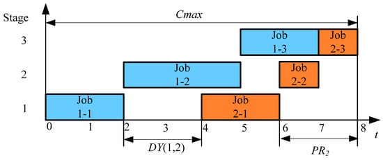
Figure 1.
The composition chart of Cmax.
2.2. Equivalent Model
Considering jobs as cities and the delay value as the distance between two cities, the NWFSP can be transformed into the ATSP. After adding virtual city/job “0”and “n + 1”, the model can be described as follows. For convenience, “0” and “n + 1” are counted as the same city, and “0” represents the starting city/job, and “n + 1” represents the ending city/job. The city/job set is .
The objective:
Subjected to:
3. The Proposed Heuristic Algorithms
The NWFSP can be transformed into the ATSP, so the path-exchange-strategy used in the Lin-Kernighan–Helsgaun (LKH) [45] algorithm is also suitable for solving NWFSP. Based on this idea, we can divide the neighborhood and construct heuristic algorithms.
3.1. Basic Neighborhood Structures
Considering the search efficiency fully, the search solution domain is initially limited to three levels, that is, Neighborhood , , . The characteristics of the three basic neighborhoods are given in Table 1. The optimum means that the solution cannot be better by exchanging areas, which are arbitrarily divided in the sequence.

Table 1.
Basic Neighborhood Features.
The neighborhood is shown in Figure 2 as an example, where and are the two area lines and the three regions are , , .
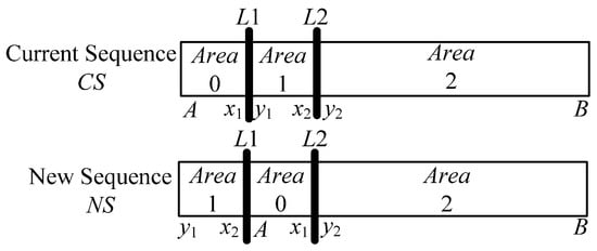
Figure 2.
An example diagram of the evolution {102} in the N2 neighborhood.
3.2. Selected Potential Sub-Neighborhoods
In order to improve the search efficiency and advance the search process in more potential sub-domains, three rules are proposed and three sub-domains are selected, namely , , and . The details are shown in Table 2. Two heuristic algorithms will be carried out along these three neighborhoods.
Table 2.
Neighborhood classification.
- Skipping consecutive area rule
Considering that the current solution sequence is almost derived from the last region-exchange operation, the combinations containing the adjacent area number pair (that is “01”, “12”, “23”, “34”) as a part do not temporarily need to test again.
- First and last job unchanged rules
From the experimental results, along the evolutionary direction, the job in last position is easier to have coincidence with the optimal solution because of being affected by values. Then is the first position. When the evolution process has advanced to a certain level, the first and last job can be fixed.
- Low-Level-neighborhood first searched rule
The lower the neighborhood level, the higher the search priority. The algorithm flow chart is shown in Figure 3. “US” is the abbreviation of “Update successfully” and “UF” is the abbreviation of “Update failed”. For ease of representation, the structure in the dashed box in Figure 3 is referred to as “PHM”.
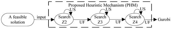
Figure 3.
The simplified search mechanism contains three neighborhoods.
3.3. Two Heuristic Algorithms
Based on the mechanism in Figure 3, it is easy to propose two heuristic algorithms according to whether the value characteristic is highlighted. The two heuristic algorithms HG1 and HG2 differ only in the first step, that is, the input feasible solutions are different. The details are shown in Figure 4. The advantage of HG1 is randomness. HG2 always takes the job with the smallest value as the final job to start the search, which is more in line with the characteristics of NWFSP and can speed up the algorithm convergence.
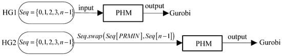
Figure 4.
Schematic diagram of the HG1 and HG2.
In order to improve the utilization of historical data and improve the efficiency of neighborhood search. According to the different characteristics of the neighborhoods of , and , corresponding search algorithms are provided one by one. They are vmcmp2, vmcmp3, and vmcmp4.
3.3.1. Local Evolutionary Algorithm in Z2
Searching the only manner {102} can improve evolution speed. Without the change of , the evaluation speed is further improved. Let the size of characterize the degree of improvement of the new sequence; the larger the value, the better the improvement.
In Figure 2, it can be seen that for the same , when and move, , , , are changed, but , remains unchanged, which can be regarded as constants. Because the first job is stored in , once the adjustment is made according to {102}, the value of the new sequence must change, and the value of will also change. As can be seen from Equation (15), in order to make full use of historical data and reduce repeated calculating, is regarded as two components. The first part and the second part are respectively represented by functions and , as shown in Equations (16) and (17).
The two-dimensional array is constructed, and the calculation result of Equation (17) is stored in the row and the column of . Such an operation can ensure that after the sequence is updated, the intermediate result only needs to recalculate part of the data. For the convenience of description, several definitions are given below.
Definition 1
(Point). Adjacent job pair makes up a point. If is a point,
is the predecessor job of
, and
is the successor job of
.
Definition 2
(Single-point Attribute (SPA)). The function value calculated by a point only or with information of a stable job. For example, function is the single-point attribute of the point
, where
is the stable job.
Definition 3
(Double-point Attribute (DPA)). The function value is calculated by two points and reflects the relationship of four related jobs. For example, function is the double-point attribute of point
and point
.
When traversing , function is associated with the attributes of job which belongs to the second point . But in essence, is still a job in . If the index number of the first job in the sequence is 0, then the index range of is (denote the index of in the sequence as , then ). Function is seen as the single-point attributes of the jobs whose index ranges from 1 to . Once is given, we can directly calculate the function . It can be seen from the characteristics of the double-point attribute that if the two points do not change, then their DPAs do not change. That is, as long as the con1 is met, the saved values in need not be updated, and the calculation speed can be increased.
The con1 is described as follows.
First, the jobs and remain in the original pair order, that is, in the sequence , and is still on the left side of .
Second, to find the value of the job and job , that is, in , x cannot be equal to or in the last operation; cannot be equal to or .
The local optimal algorithm (Algorithm 1) for is described as follows.
| Algorithm 1. vmcmp2(con1)// Search {102} only |
| Step 1. compute all the SPAs in CS, that is, all the |
| Step 2. compute all the DPAs in CS, that is, all the |
| Step 3. //Save the best positions to which provide the |
| Step 4. if |
| L1 = and L2 = |
| CS=CS ({102})//Perform operation {102} on CS to update CS |
| update (); //Recalculate all the f values |
| update (, ); // Recalculate g values that do not meet con1 |
| jump to Step 3 |
| end if |
| else// CS is the best of Z2 now |
| Stop searching in Z2 |
| end else |
3.3.2. Local Evolutionary Algorithm in Z3
Since the first job and the last job are constant, the point attribute can be used with the historical data to optimize the algorithm. Figure 5 shows the evolution form of “0213”, from which Equation (20) can be obtained.
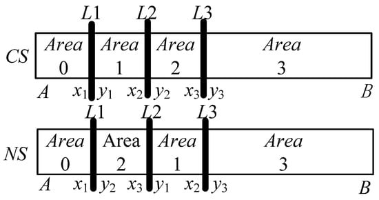
Figure 5.
The evolution graph in Z3.
Where represents the sum of the delay values of all the jobs from the job to the job in the current sequence. Equation (20) is the sum of the expressions in the three brackets, and the three sub-expressions, which can be seen as DPAs are in a rotation-symmetric relationship. Parentheses 1 and 2 can share the function . Parenthesis 3 is denoted as function .
and are considered as functions of the job numbers and the function values are saved. See Equations (21) and (22) for details.
Compute and save each value to the row, column of the two-dimensional array . Assume point1 , point2 , point3 , then Equation (20) can be replaced by Equation (23) to reduce double counting.
In contrast to the search in , there is only one combination to try, so compute all and choose the biggest improvement. If all is computed but only updated at most once, the utilization rate of historical data is too low. Then Multiple Iterations in One step (MIO) is proposed to improve this situation.
Traverse the Z3 neighborhood of CS, the specific method is to calculate by Formula 23, and save all the values greater than 0 in . In Figure 6, is a multiset that sorts the results according to its values, from largest to smallest, and itRS7 is the iterator of .
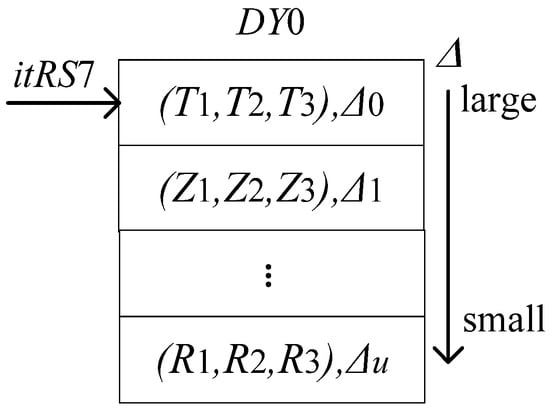
Figure 6.
Data storage manner of
.
Suppose there is a NWFSP with , and the is shown in Figure 6. As shown in Figure 7, its current solution is .
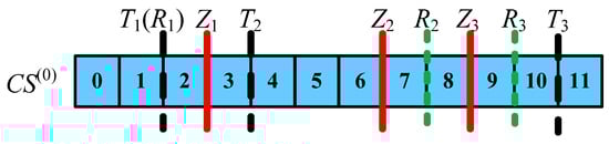
Figure 7.
Data characteristics of the 0 iteration of CS.
Take out the element pointed to by the iterator , that is .Then the evolution process can be seen in Figure 8. The indices of points (1, 2), (3, 4), (10, 11) in the sequence are respectively recorded as . In Figure 6, means .
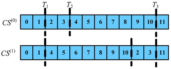
Figure 8.
One iteration by the way of (T1, T2, T3).
Because of the constant last job, the is constant too. Then the essence of every evolution manner is the change of boundary values. Combining Figure 6 and Figure 7, we can draw the conclusions of Table 3.
Table 3.
Changed Paths of Boundary Values.
It is easy to see from Table 3 that no matter how many iterations are completed, as long as the changed path of boundary values still exist, evolution in this direction will succeed.
It can be seen from Figure 9 that after two iterations, the corresponding point of cannot be found in at this time, so it cannot be evolved in this way. Next, derive the conditions con2 whose paths still exist after iterations, as shown in Table 4.
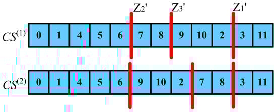
Figure 9.
Two iterations by the way of (T1, T2, T3) and (Z1, Z2, Z3).
Table 4.
Conditions for con2.
Traverse and determine whether each element meets the con2 in turn. If one is satisfied, it is applicable and the iteration can be completed directly. Therefore, is calculated only once, and there is a chance to iterate multiple times. The algorithm (Algorithm 2) vmcmp3(con2) suitable for is described as follows.
| Algorithm 2. vmcmp3(con2) |
| Step 1. Input , record Loc (j, ) and save them to vector k1, Let its jth element, k1(j) to save the location of job j in |
| Step 2. flag = 0// Set the initial value of the flag |
| Step 3. Compute and save , , then compute and save them to multiset DY0 when . |
| Step 4. if (DY0.size()! = 0) // if DY0 is not empty |
| for itRS7 = DY0.begin() to DY0.end ()-1)// Traverse DY0 by itRS7 |
| if(con2) //If con2 is met |
| CS= update (itRS7, {2013}, CS);// According the locations |
| //provided by DY0, give CS a {2013} operation |
| flag=1// Updated successfully |
| update (Loc (j, CS)); // Save the new correspondence of location //and job number |
| end if(con2) |
| end for |
| end if |
| else |
| flag=2 |
| end else |
| if flag==1 // When update successfully |
| jump to Step2 |
| end if |
| else // When update failed |
| Stop searching in Z3 |
| end else |
3.3.3. Local Evolutionary Algorithm in Z4
Experiments show that the combination {03214} has a higher hit rate. Its main feature is that the first and last jobs are not changed. The Figure 10 shows the evolution form.
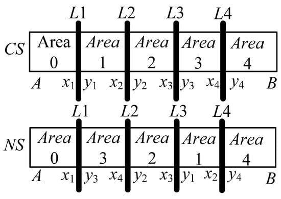
Figure 10.
Evolution graph in Z4.
Still, start with the expression of , specific as shown in Equations (24)–(26).
Similarly, using Equation (27) to uniformly calculate the two parts separated by parentheses in Equation (26) can simplify the calculation. Let be here.
Compute all the results by Equation (27) and save them in multiset .
Use two iterators, and to traverse . Then select all the elements that meet the condition of con3, and store them in multiset . See Figure 11 and Figure 12 for details.
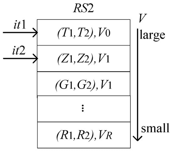
Figure 11.
Data storage diagram in RS2.
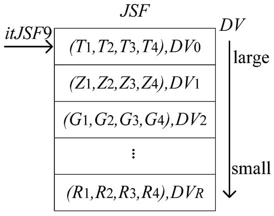
Figure 12.
Data storage diagram in JSF.
collects all successful evolution paths. Its iterator is itRS9 in Figure 12 (). Suppose the variables saved by a single element in are and , then the conditions for con3 to be established are shown in Table 5.
Table 5.
Conditions for con3.
Similarly, use MIO Strategy to construct an algorithm (Algorithm 3) to speed up the search process.
| Algorithm 3. vmcmp4(con3, con4) |
| Step 1. Input , record Loc (j, ) and save them to vector k1, Let its jth element, k1(j) to save the location of job j in |
| Step 2. flag = 0// Set the initial value of the flag |
| Step 3. for = 0 to n-4 // The union of the ranges L1 and L2 |
| for = 3 to n − 1// The union of the ranges L3 and L4 |
| cmpRS2(,)//compute the DPAs of (, , , ) and save them in RS2 |
| end for // End the inner loop |
| end for// End outer loop |
| Step 4. it1begin = RS2.begin() |
| it2begin = it1 + 1 // Assign initial values to iterators it1 and it2 |
| for it1 = it1begin to it1end |
| for it2 = it2begin to it2end // Double loop for traverse RS2 |
| if (con3(it1, it2)) //If the elements pointed to by it1 and it2 satisfy con3 |
| JSF. insert (it1, it2)//Save the evolution path provided |
| //by the elements which are pointed to by it1 and it2 in JSF |
| end if |
| end for// End the inner loop |
| end for// End outer loop |
| Step 5. if (JSF. size ()0)//If JSF is not empty, it means that can be |
| //updated in its neighborhood Z4 |
| for itJSF9 = JSF. begin () to JSF. end ()−1 //Traverse multiset JSF |
| //which is the neighborhood Z4 of |
| if (con4(itJSF9))//If the element pointed to by itJSF9 satisfies the con4 |
| CS = update (JSF9, {03214}, CS)//Update CS as specified by JSF9 |
| update (Loc (j, CS)); // Save the new correspondence of |
| //location and job number |
| flag = 1; // Assign 1 to the flag bit |
| end if |
| end for |
| end if |
| else |
| flag = 2 |
| end else |
| if flag == 1// If there is an update in this round |
| jump to Step2 |
| end if |
| else// This round of searching this in Z4 has not been updated |
| Stop searching in Z4 |
| end else |
Let the condition that satisfies MIO in Z4 be con4. If con4 in the algorithm is to be established, two conditions must be met, as shown in Table 6.
Table 6.
Conditions for con3.
3.4. Experimental Results of the Two Heuristic Algorithms
Use HG1 and HG2 to solve Tailard (TA) benchmark. Then record the calculation results in Table 7. The heuristic algorithms were coded in C++. All the experiments executed in Windows 10 on a desktop PC with an 11th Gen Intel(R) Core (TM) i7-1165G7 (2.80GHz) processor and 16.0 GB RAM. The calculation formula of RPI (Relative Percentage Increase) and are shown in Equations (28) and (29), where refers to the optimal of instance a1. refers to the result of algorithm i1 to solve the instance a1.
Table 7.
Results of HGs on Tailard Benchmark (TA).
In Table 7, HG2 has a smaller value than HG1 in all scale instances; its fluctuation range is from 0.8% to 2.58%, the maximum value of 2.58% appears on the small-scale instances (scale is 20 × 10), while its value on the largest-scale instances (500 × 20) is only 1.28%. On the whole, it performs better for large-scale instances. The average is 1.30%, and the fluctuation is not large, indicating that the algorithm has strong local search ability, and can quickly converge to a local optimal solution regardless of the scale, with stable performance.
It can be seen from Table 7 that out of 120 instances, HG1 only exceeds HG2 in 6 instances (the part in bold in the table). Therefore, for the goal of approximating the optimal value, the effect of the HG2 algorithm constructed by introducing the value is much better than that of HG1, and even HG2 directly obtains the optimum on some small-scale instances (the part in italics in the table). Taking “TA 05” as an example, its Gantt chart is shown in Figure 13. If the result of HG1 is imported into Gurobi, another set of optimal solution sequences can be obtained. This Gantt chart is shown in Figure 14. Therefore, the use of different heuristic algorithms is effective for the breadth search. The same job-blocks in the HG1 sequence and the HG2 sequence can also be considered as high-quality structures by comparing them with the optimal solution sequence. Therefore, the heuristic algorithms can easily construct multiple high-quality solutions. Arrange the jobs according to their values from small to large, take them as the last job in turn, and then perform the PHM operation.
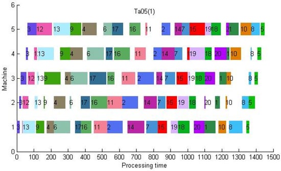
Figure 13.
The Gantt chart of TA05 by HG2 (makespan = 1449).
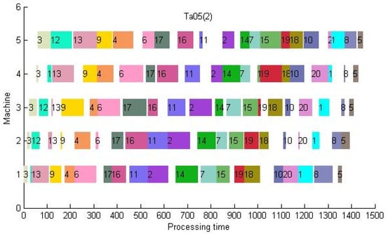
Figure 14.
The Gantt chart of TA05 by Gurobi with HG1 (makespan = 1449).
Similarly, we used HG1 and HG2 to solve Reeves (REC) benchmark. The results are recorded in Table 8.
Table 8.
Results of HGs on REC.
On this benchmark, the values obtained by HG2 are also better than that obtained by HG1. Except for REC11, HG1 does not get a better than HG2, and HG2 even gets the optimal solution on REC03. Obviously, the effect of HG2 is better than that of HG1, so HG2 was selected to participate in the calculation in subsequent studies.
4. Solving the Model with Matheuristic Algorithms
4.1. Test on Small-Scale Instances with MTZ Model
When Gurobi solves the NWFSP problem, if all constraints are added directly at the beginning of the optimization, the solution performance will be greatly reduced, for example, when the famous Miller-Tucker-Zemlin model [46] (Formulas (6)–(12), Equation (14) and Formula (30)) is used directly. However, the model has high research value [47]. We combine the heuristic algorithm to improve the efficiency.
Using Gurobi (The version is 9.1.2.) to solve this model directly, the results are shown in Table 9 and Table 10. Among them, TA02 takes a longer time, and TA37 has not completed the calculation within 36,000 s.
Table 9.
Results of MTZ model on REC (tolerance is 10−4).
Table 10.
Results of MTZ model on TA01–TA60 (tolerance is 10−4).
We select those instances (T > 7s) with longer solution times, and combine heuristics to improve efficiency. NA (not a number) indicates that the calculation has not been completed within 36,000 s.
The method of importing only the result (named as S2) of HG2 as an initial feasible solution to the optimizer is called MH2, then the solution efficiency for instances marked in italics is improved.
Since NWFSP is solved by transforming it into an ATSP problem, i.e., the solution satisfies the characteristic of a “loop”. We choose the last three jobs in S2 to join the first three jobs to form a test sequence. The test sequence is shown in Formula (31).
Using adjacent job pairs in the test sequence as constraints one by one, test the running time separately (if a single test exceeds 10s, test the next job pair or end the test). Among the results satisfying RPI = 0, select the best (the one with the shortest running time) as the improvement value and store it in the IMH2 column of Table 11. It can be seen that the speed of solving other instances in Table 11 are also improved to varying degrees (the last column in Table 11). This shows that the matheuristic method is effective.
Table 11.
Comparison Results of MH2, IMH2 and MTZ only (tolerance is 10−4).
4.2. Comparison Results of MH2 and Other Algorithms
While we used the matheuristic in the previous subsection to improve the efficiency of the MTZ model, the strategy of dynamically adding constraints using callback functions when solving large-scale instances has greater advantages. We use this strategy to solve the proposed model (Formula 6-Formula 14), also naming the mathematic algorithm that introduces HG2 as MH2. The comparison results of MH2, DWWO [32], SWWO [34], and IDMBO [37] are shown in Table 12 and Table 13.
Table 12.
Comparison Results of MH2, IDMBO, DWWO, and SWWO on TA.
Table 13.
Comparison Results of MH2, IDMBO, DWWO, and SWWO on REC.
These comparison algorithms are the main intelligent algorithms for solving NWFSP problems in recent years (2018–2020). We carefully reproduced the algorithms following the steps in the literature and set the parameters as required therein. Considering the uniformity, the condition for terminating the program was selected from the literature [34], that is, the upper limit of the running time is n × m × 90/2. Each algorithm takes five independent runs for each instance, according to [37]. Calculate with Equations (32)–(34) and fill in Table 12 and Table 13 with the results. All algorithms are programmed in C++ (Visual studio 2019) and run on the same desktop PC with an 11th Gen Intel(R) Core (TM) i7-1165G7 (2.80GHz) processor and 16.0 GB RAM.
The minimum and average values of five independent runs of algorithm i1 on instance a1 are denoted as and . , , and represent the arithmetic mean of , , and Time of the same scale, respectively, and represents the result of the ctth running of the algorithm i1 on the instance a1.
Table 12 shows the test results of the four algorithms on the Tailard benchmark, in which the first column records the averages of the optimal values for instances of the same size. The proposed matheuristic algorithm MH2 achieves the optimal solutions in all instances. Even for the largest instances (500 × 20), the average running time is 112.82 s. The running time of a single instance with a scale of less than or equal to 200 is short, ranging from tens of milliseconds to a dozen seconds. Therefore, the algorithm is efficient and feasible. MH2 does not contain random parameters, so the SD value is always 0, and the algorithm is stable.
It can be seen from column that when the job size of the Tailard benchmark is greater than or equal to 50, the three metaheuristic algorithms cannot obtain an optimal solution within n × m × 90/2, even if they are run 5 times independently. As the job size increases, the difference between the output value and the optimal solution also increases. In the case of SWWO [34], which has the best comprehensive ability among the three metaheuristics, when the scale is 200 × 20, the difference between the average output solution and the average optimum is about 200 (19788.4 × 1.00%). The metaheuristic algorithm needs more running time to get a better solution, and its convergence speed is not as fast as MH2.
Table 13 shows the results of the four algorithms for solving the small-scale benchmark Reeves, where the first column records the optimal values of the instances. The operating efficiency of the MH2 algorithm is the highest, and the optimal value of any REC instance can be obtained within 1 s. The second is the SWWO algorithm [34], which can find the optimal solution except REC39 and REC41.
In summary, when n < 30, the difference between the four algorithms is not big, and the optimal solutions can basically be found. When n = 50, the search ability of the two swarm intelligence algorithms, IDMBO [37] and DWWO [32], are not as good as that of the adaptive algorithm SWWO [34]. SWWO [34] has the ability to find the optimal solution for an instance of size n = 75 in 67.5 s. To a certain extent, it verifies the NWFSP, which is more suitable for a search mechanism with more local search than global search. Comparing Table 7, it can be seen that when the scale is increased to 200 × 10 and 500 × 20, the of the heuristic algorithm HG2 is 0.92% and 1.28% respectively, that is, the search performance also exceeds the other three intelligent algorithms. This shows that it is feasible to perform a local search with the job with the smallest value in the job set as the end job.
4.3. Results and Discussion
- This study determined the optimal solutions for 141 instances on the Tailard and Reeves benchmarks. Further analysis based on the optimal solutions can verify the validity of the proposed heuristic rule. The final job of the optimal solution is often the job with a smaller value.
Step 1. Arrange the jobs according to their values from small to large. The corresponding rank with the smallest value is 0.
Step 2. Record the Final Job Ranking (FJR) of each optimal sequence. See Table 14 for details.
Table 14.
The FJR of TA.
It can be seen from Table 14 that the FJR values of the instances are distributed between 0 and 30, and the case of “” accounts for 55%, as shown in Figure 15.
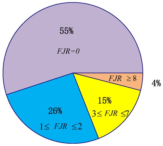
Figure 15.
The PPRK value distribution ratio chart.
- The heuristic algorithm can effectively guide the optimization direction of the optimizer and improve the solution rate of complex models. Making full use of the advantages of both can not only find more optimal solutions, but also expand the application range of exact algorithms and obtain high-quality solutions that cannot be obtained by metaheuristic algorithms. Two different optimal sequences are obtained on REC05, REC09, TA01, TA03, TA05, TA21, TA32, TA33, TA34, TA35, TA41, TA42, TA44, TA45 and TA46, respectively.
5. Conclusions and Future Work
5.1. Conclusions
This paper studied the characteristics of NWFSP and verified that the value is an important indicator of a job. Taking the job with the smaller value as the final job has a higher probability of obtaining the optimal solution.
Along the evolutionary direction of HG1 and HG2, different optimal values can be obtained. This shows that HG1 and HG2 as initial solutions have good dispersion. The rule and , , neighborhoods are also fit to be components of intelligent algorithms.
If the job with the smallest value is placed in the last position, and then the neighborhood search is expanded step by step (search , , in turn), the iterative results are often consistent with the optimal solutions in the first few and last few jobs. Bringing these into the optimizer increases the model solution rate.
Experiments show that the optimal values of the two benchmarks (REC and TA) can be obtained by using the Matheuristic MH2 method within an acceptable time (the running time of a single instance with a scale of 500 × 20 is less than 134 s). This shows that the algorithm is feasible.
5.2. Future Work
- Considering the computing power of personal laptops, this paper only studies the three-level neighborhood division method, and initially realizes the idea of gradually expanding the search domain of NWFSP. However, for large-scale instances, the coverage of the three-level neighborhood is not enough, so the effect has a certain dependence on the initial value. In the future, more levels of neighborhood division methods and corresponding neighborhood search methods can be further studied to improve the stability of the algorithm.
- The scope of application of the proposed rules and neighborhood partitioning strategies can be generalized in the future, and they can be embedded in the framework of metaheuristic algorithms to solve NWFSP. In the past, heuristic algorithms were mostly used to construct high-quality solutions, but the rules proposed in this paper satisfy the conditions of participating in all stages. The interaction method between heuristic rules driven by problem features and metaheuristics with the advantage of generality can be further studied to improve the ability of metaheuristics to solve NWFSP.
- In real production, distributed requirements are becoming more and more extensive.
Since the matheuristic solves the NWFSP problem well, it can also be studied to solve the Distributed No-wait Flowshop Scheduling Problem (DNWFSP). On the one hand, it is possible to study the method of building a simplified model of DNWFSP based on the existing NWFSP model; on the other hand, how to use the obtained heuristic rules to guide the optimization direction of the optimizer, improve the speed of solving large-scale instances and expand the application range of exact algorithms is also a future research direction.
Author Contributions
Software, Y.G.; validation, Y.G.; writing—original draft preparation, Y.G. and Z.W.; writing—review and editing, Z.W.; supervision, L.G. and X.L.; project administration, L.G. and X.L.; funding acquisition, L.G. All authors have read and agreed to the published version of the manuscript.
Funding
This research received no external funding.
Institutional Review Board Statement
Not applicable.
Informed Consent Statement
Not applicable.
Data Availability Statement
The study did not report any data.
Conflicts of Interest
The authors declare no conflict of interest.
References
- Arik, O.A. Genetic algorithm application for permutation flow shop scheduling problems. Gazi Univ. J. Sci. 2022, 35, 92–111. [Google Scholar] [CrossRef]
- Red, S.F. An effective new heuristic algorithm for solving permutation flow shop scheduling problem. Trans. Comb. 2022, 11, 15–27. [Google Scholar]
- Li, W.M.; Han, D.; Gao, L.; Li, X.Y.; Li, Y. Integrated production and transportation scheduling method in hybrid flow shop. Chin. J. Mech. Eng. 2022, 35, 12. [Google Scholar] [CrossRef]
- Jemmali, M.; Hidri, L.; Alourani, A. Two-stage hybrid flowshop scheduling problem with independent setup times. Int. J. Simul. Model. 2022, 21, 5–16. [Google Scholar] [CrossRef]
- Zhang, J.; Ding, G.F.; Zou, Y.S.; Qin, S.F.; Fu, J.L. Review of job shop scheduling research and its new perspectives under industry 4.0. J. Intell. Manuf. 2019, 30, 1809–1830. [Google Scholar] [CrossRef]
- Sun, Y.; Pan, J.S.; Hu, P.; Chu, S.C. Enhanced equilibrium optimizer algorithm applied in job shop scheduling problem. J. Intell. Manuf. 2022. Available online: https://www.webofscience.com/wos/alldb/full-record/WOS:000739739300001 (accessed on 1 January 2022). [CrossRef]
- Aghighi, S.; Niaki, S.T.A.; Mehdizadeh, E.; Najafi, A.A. Open-shop production scheduling with reverse flows. Comput. Ind. Eng. 2021, 153, 107077. [Google Scholar] [CrossRef]
- Ozolins, A. Dynamic programming approach for solving the open shop problem. Cent. Europ. J. Oper. Res. 2021, 29, 291–306. [Google Scholar] [CrossRef]
- Callahan, J.R. The Nothing Hot Delay Problems in the Production of Steel. Ph.D. Dissertation, Department of Mechanical & Industrial Engineering, Toronto University, Toronto, ON, Canada, 1971. [Google Scholar]
- Tang, J.F.; Song, J.W. Discrete particle swarm optimisation combined with no-wait algorithm in stages for scheduling mill roller annealing process. Int. J. Comput. Integr. Manuf. 2010, 23, 979–991. [Google Scholar] [CrossRef]
- Höhn, W.; Jacobs, T.; Megow, N. On Eulerian extensions and their application to no-wait flowshop scheduling. J. Sched. 2012, 15, 295–309. [Google Scholar] [CrossRef]
- Yuan, H.W.; Jing, Y.W.; Huang, J.P.; Ren, T. Optimal research and numerical simulation for scheduling No-Wait Flow Shop in steel production. J. Appl. Math. 2013, 2013, 498282. [Google Scholar] [CrossRef]
- Reklaitis, G.V. Review of scheduling of process operations. AIChE Symp. Ser. 1982, 78, 119–133. [Google Scholar]
- Hall, N.G.; Sriskandarajah, C. A survey of machine scheduling problems with blocking and no-wait in process. Oper. Res. 1996, 44, 510–525. [Google Scholar] [CrossRef]
- Babor, M.; Senge, J.; Rosell, C.M.; Rodrigo, D.; Hitzmann, B. Optimization of No-Wait Flowshop Scheduling Problem in Bakery Production with Modified PSO, NEH and SA. Processes 2021, 9, 2044. [Google Scholar] [CrossRef]
- Hsu, V.N.; de Matta, R.; Lee, C.Y. Scheduling patients in an ambulatory surgical center. Nav. Res. Logist. 2003, 50, 218–238. [Google Scholar] [CrossRef]
- Mannino, C.; Mascis, A. Optimal real-time traffic control in metro stations. Oper. Res. 2009, 57, 1026–1039. [Google Scholar] [CrossRef]
- Tomazella, C.P.; Nagano, M.S. A comprehensive review of Branch-and-Bound algorithms: Guidelines and directions for further research on the flowshop scheduling problem. Expert Syst. Appl. 2020, 158, 113556. [Google Scholar] [CrossRef]
- Graham, R.; Lawler, E.; Lenstra, J.; Kan, A. Optimization and approximation in deterministic sequencing and scheduling: A survey. Ann. Math. 1979, 5, 287–326. [Google Scholar]
- Garey, M.R.; Johnson, D.S. Computers and Intractability: A guide to the Theory of NP-Completeness; W.H. Freeman and Company: New York, NY, USA, 1979. [Google Scholar]
- Papadimitriou, C.H.; Kanellakis, P.C. Flowshop scheduling with limited temporary storage. J. ACM 1980, 27, 533–549. [Google Scholar] [CrossRef] [Green Version]
- Bonney, M.C.; Gundry, S.W. Solutions to the constrained flowshop sequencing problem. J. Oper. Res. Soc. 1976, 27, 869–883. [Google Scholar] [CrossRef]
- King, J.R.; Spachis, A.S. Heuristics for flowshop scheduling. Int. J. Prod. Res. 1980, 18, 343–357. [Google Scholar] [CrossRef]
- Gangadharan, R.; Rajendran, C. Heuristic algorithms for scheduling in the no-wait flowshop. Int. J. Prod. Econ. 1993, 32, 285–290. [Google Scholar] [CrossRef]
- Laha, D.; Chakraborty, U.K. A constructive heuristic for minimizing makespan in no-wait flow shop scheduling. Int. J. Adv. Manuf. Technol. 2009, 41, 97–109. [Google Scholar] [CrossRef]
- Ying, K.C.; Lu, C.C.; Lin, S.W. Improved exact methods for solving no-wait flowshop scheduling problems with due date constraints. IEEE Access 2018, 6, 30702–30713. [Google Scholar] [CrossRef]
- Land, A.H.; Doig, A.G. An automatic method of solving discrete programming problems. Econometrica 1960, 28, 497–520. [Google Scholar] [CrossRef]
- Pei, Z.; Zhang, X.F.; Zheng, L.; Wan, M.Z. A column generation-based approach for proportionate flexible two-stage no-wait job shop scheduling. Int. J. Prod. Res. 2020, 58, 487–508. [Google Scholar] [CrossRef]
- Allahverdi, A. A survey of scheduling problems with no-wait in process. Eur. J. Oper. Res. 2016, 255, 665–686. [Google Scholar] [CrossRef]
- Pan, Q.K.; Wang, L.; Tasgetiren, M.F.; Zhao, B.H. A hybrid discrete particle swarm optimization algorithm for the no-wait flow shop scheduling problem with makespan criterion. Int. J. Adv. Manuf. Technol. 2008, 38, 337–347. [Google Scholar] [CrossRef]
- Engin, O.; Guclu, A. A new hybrid ant colony optimization algorithm for solving the no-wait flow shop scheduling problems. Appl. Soft. Comput. 2018, 72, 166–176. [Google Scholar] [CrossRef]
- Zhao, F.Q.; Liu, H.; Zhang, Y.; Ma, W.M.; Zhang, C. A discrete water wave optimization algorithm for no-wait flow shop scheduling problem. Expert Syst. Appl. 2018, 91, 347–363. [Google Scholar] [CrossRef]
- Zhao, F.Q.; Qin, S.; Yang, G.Q.; Ma, W.M.; Zhang, C.; Song, H.B. A factorial based particle swarm optimization with a population adaptation mechanism for the no-wait flow shop scheduling problem with the makespan objective. Expert Syst. Appl. 2019, 126, 41–53. [Google Scholar] [CrossRef]
- Zhao, F.Q.; Zhang, L.X.; Liu, H.; Zhang, Y.; Ma, W.M.; Zhang, C.; Song, H.B. An improved water wave optimization algorithm with the single wave mechanism for the no-wait flow-shop scheduling problem. Eng. Optimiz. 2019, 51, 1727–1742. [Google Scholar] [CrossRef]
- Zhao, F.Q.; Qin, S.; Zhang, Y.; Ma, W.M.; Zhang, C.; Song, H.B. A hybrid biogeography-based optimization with variable neighborhood search mechanism for no-wait flow shop scheduling problem. Expert Syst. Appl. 2019, 126, 321–339. [Google Scholar] [CrossRef]
- Zhu, H.H.; Qi, X.M.; Chen, F.L.; He, X.; Chen, L.F.; Zhang, Z.Y. Quantum-inspired cuckoo co-search algorithm for no-wait flow shop scheduling. Appl. Intell. 2019, 49, 791–803. [Google Scholar] [CrossRef]
- Zhang, S.J.; Gu, X.S.; Zhou, F.N. An improved discrete migrating birds optimization algorithm for the no-wait flow shop scheduling problem. IEEE Access 2020, 8, 99380–99392. [Google Scholar] [CrossRef]
- Lai, R.S.; Gao, B.; Lin, W.G. Solving no-wait flow shop scheduling problem based on discrete wolf pack algorithm. Sci. Program. 2021, 2021, 4731012. [Google Scholar] [CrossRef]
- Burke, E.K.; Kendall, G.; Soubeiga, E. A tabu-search hyperheuristic for timetabling and rostering. J. Heuristics 2003, 9, 451–470. [Google Scholar] [CrossRef]
- Della Croce, F.; Salassa, F. A variable neighborhood search based matheuristic for nurse rostering problems. Ann. Oper. Res. 2014, 218, 185–199. [Google Scholar] [CrossRef]
- Kramer, R.; Subramanian, A.; Vidal, T.; Cabral, L.D.F. A matheuristic approach for the Pollution-Routing Problem. Eur. J. Oper. Res. 2015, 243, 523–539. [Google Scholar] [CrossRef] [Green Version]
- Hong, J.; Moon, K.; Lee, K.; Lee, K.; Pinedo, M.L. An iterated greedy matheuristic for scheduling in steelmaking-continuous casting process. Int. J. Prod. Res. 2021, 60, 623–643. [Google Scholar] [CrossRef]
- Lin, S.W.; Ying, K.C. Optimization of makespan for no-wait flowshop scheduling problems using efficient matheuristics. Omega-Int. J. Manag. Sci. 2016, 64, 115–125. [Google Scholar] [CrossRef]
- Bagchi, T.P.; Gupta, J.N.; Sriskandarajah, C. A review of TSP based approaches for flowshop scheduling. Eur. J. Oper. Res. 2006, 169, 816–854. [Google Scholar] [CrossRef]
- Helsgaun, K. An effective implementation of the Lin-Kernighan traveling salesman heuristic. Eur. J. Oper. Res. 2000, 126, 106–130. [Google Scholar] [CrossRef] [Green Version]
- Gouveia, L.; Pires, J.M. The asymmetric travelling salesman problem and a reformulation of the Miller-Tucker-Zemlin constraints. Eur. J. Oper. Res. 1999, 112, 134–146. [Google Scholar] [CrossRef]
- Campuzano, G.; Obreque, C.; Aguayo, M.M. Accelerating the Miller-Tucker-Zemlin model for the asymmetric traveling salesman problem. Expert Syst. Appl. 2020, 148, 113229. [Google Scholar] [CrossRef]
Publisher’s Note: MDPI stays neutral with regard to jurisdictional claims in published maps and institutional affiliations. |
© 2022 by the authors. Licensee MDPI, Basel, Switzerland. This article is an open access article distributed under the terms and conditions of the Creative Commons Attribution (CC BY) license (https://creativecommons.org/licenses/by/4.0/).