Khalil New Generalized Weibull Distribution Based on Ranked Samples: Estimation, Mathematical Properties, and Application to COVID-19 Data

Abstract

In this paper, a five-parameter distribution, Khalil’s new generalized Weibull distribution, is defined and studied in detail. Some mathematical and statistical functions are studied. The effects of shape parameters on skewness and kurtosis are studied. Extensions for density and distribution functions are provided. Estimation of the intended model parameters based on ranked samples is investigated. The behavior of the maximum likelihood estimators is examined using a Monte Carlo simulation. In order to predict unique symmetric and asymmetric patterns and illustrate the applicability and potential of the intended distribution, a COVID-19 dataset is analyzed. The goodness-of-fit results of the new generalized Weibull model of Khalil are compared with some other models. Finally, we make some concluding remarks.

1. Introduction

In order to achieve the goals that the researcher has set for his or her research, the researcher must collect data and information about that research. Since some data may be difficult to obtain or unacceptable due to cost, labor, and time constraints, he must choose the sampling method that will guarantee that he will achieve the research objectives with the least amount of time and expense—or, in many practical cases, it is not possible to obtain true measurements of the variables of interest, which is expensive and therefore a waste of time. To solve these problems, it is necessary to use a sampling method that ensures that time, effort, and cost are reduced in obtaining data.

The Ranked Set Sampling (RSS) method was proposed by McIntyre [1] as an inexpensive and effective method for estimating pasture yield. Although the RSS method is not parametric, many authors have used it to estimate parameters for many distributions and have demonstrated that its estimates are more effective than estimates based on simple random sampling and the same sample size. More detailed information can be found in [2,3,4,5]. Therefore, the aim of this work was to estimate the parameters of the Khalil new generalized Family-Weibull Distribution (KHGWD) considering ordered groups.

We now briefly introduce the RSS strategy used in the supplements. Consider an absolutely continuous random variable $\chi$ with the cumulative distribution function (CDF) and the probability density function (PDF). Then, a simple random sample of size n derived from the random variable $\chi$ is denoted by $\chi =\{{\chi }_{i:n},i=1,\dots ,n\}$. Suppose further that a random sample of size $n^2$ is selected and randomly divided into n groups of equal size. Then, RSS is observed according to the following pattern:

(1)	$\underline{{\chi }_{(1:n)1}}$	${\chi }_{(2:n)1}$	…	${\chi }_{(n:n)1}$	→	${\chi }_{1,1}={\chi }_{(1:n)1}$
(2)	${\chi }_{(1:n)2}$	$\underline{{\chi }_{(2:n)2}}$	…	${\chi }_{(n:n)2}$	→	${\chi }_{2,2}={\chi }_{(2:n)2}$
.	$.$	$.$		$.$		$.$
.	$.$	$.$		$.$		$.$
.	$.$	$.$		$.$		$.$
(n)	${\chi }_{(1:n)n}$	${\chi }_{(2:n)n}$	…	$\underline{{\chi }_{(n:n)r}}$	→	${\chi }_{n,n}={\chi }_{(n:n)n}$

The RSS vector of observations is given by ${\chi }_{j,i},i=1,\dots ,n,j=1,\dots ,n$, where ${\chi }_{j,i}$ is the statistic of order ith in the group jth based on a given simple random sample of size n. Then, as is well known, the PDF of ${\chi }_{j,i}$ is

$$\begin{array}{c}\hfill f_{j,i}\left(x\right)=\frac{n!}{(i-1)!(n-i)!}f\left(x\right){\left(F\left(x\right)\right)}^{i-1}{\left(1-F\left(x\right)\right)}^{n-i},j,i=1,\dots ,n.\end{array}$$

(1)

For more details, see Arnold et al. [6].

Next, Najma et al. [7] proposes a new method to extend the family of lifetime distributions. The method is called Khalil new generalized family of distributions. For any baseline CDF $G\left(x\right)$ and a PDF $g\left(x\right)$, the CDF and the PDF of the new generalized family of Khalil distributions are respectively given by

$$\begin{array}{c}\hfill F(x;\alpha ,\beta )=\frac{e^{-\alpha G{\left(x\right)}^{\beta }}-1}{e^{-\alpha }-1},x\in \mathbb{R};\alpha ,\beta >0,\end{array}$$

(2)

and

$$\begin{array}{c}\hfill f(x;\alpha ,\beta )=\frac{\alpha \beta e^{-G{\left(x\right)}^{\beta }\alpha }g\left(x\right)G{\left(x\right)}^{\beta -1}}{1-e^{-\alpha }},x\in \mathbb{R};\alpha ,\beta >0,\end{array}$$

(3)

where $\alpha$ and $\beta$ are the scale and shape parameters, respectively.

In 1939, Swedish scientist Waloddi Weibull established the Weibull distribution in a study of the breaking strength of instruments. The Weibull distribution is one of the most commonly used failure models. The Weibull distribution is used to simulate many probabilistic applications; this is due to its unique symmetric and asymmetric patterns. The distribution has several desirable properties, acceptable physical interpretations, and the ability to fit the failure rates of various systems, whether those rates are high, low, or constant.

Let X be a random variable (R.V.) that follows the Weibull distribution with three parameters $(\lambda ,\mu ,\nu )$, then its CDF, denoted by $G(x;\lambda ,\mu ,\nu ),$ is given by

$$\begin{array}{c}\hfill G(x;\lambda ,\mu ,\nu )=1-e^{-{\left(\frac{x-\nu }{\mu }\right)}^{\lambda }},x\ge \nu ;\lambda ,\mu ,\nu >0.\end{array}$$

(4)

Here, $\nu >0$ is the location parameter, $x\ge \nu$, $\lambda >0$, and $\mu >0$ are the shape and the scale parameter, respectively. The corresponding PDF, denoted by $g(x;\lambda ,\mu ,\nu ),$ is given by

$$\begin{array}{c}\hfill g(x;\lambda ,\mu ,\nu )=\frac{\lambda }{\mu }{\left(\frac{x-\nu }{\mu }\right)}^{\lambda -1}{e}^{-{\left(\frac{x-\nu }{\mu }\right)}^{\lambda }},x\ge \nu ;\lambda ,\mu ,\nu >0.\end{array}$$

(5)

2. The Khalil New Generalized Family-Weibull Distribution (KHGWD)

Take $G\left(x\right)$ and $g\left(x\right)$ in Equations (2) and (3) as $G(x;\lambda ,\mu ,\nu )$ of Equation (4) and $g(x;\lambda ,\mu ,\nu )$ of Equation (5), respectively. The CDF and the PDF of KHGWD are respectively given by

$$\begin{array}{c}\hfill F(x;\alpha ,\beta ,\lambda ,\mu ,\nu )=\frac{1-e^{-\alpha {\left(1-e^{-{\left(\frac{x-\nu }{\mu }\right)}^{\lambda }}\right)}^{\beta }}}{1-e^{-\alpha }},\end{array}$$

(6)

and

$$\begin{array}{c}\hfill f(x;\alpha ,\beta ,\lambda ,\mu ,\nu )=\frac{\alpha \beta \lambda {\left(\frac{x-\nu }{\mu }\right)}^{\lambda -1}{\left(1-e^{-{\left(\frac{x-\nu }{\mu }\right)}^{\lambda }}\right)}^{\beta -1}{e}^{-{\left(\frac{x-\nu }{\mu }\right)}^{\lambda }-\alpha {\left(1-e^{-{\left(\frac{x-\nu }{\mu }\right)}^{\lambda }}\right)}^{\beta }}}{\mu \left(1-e^{-\alpha }\right)},\end{array}$$

(7)

where $x\ge \nu$, $\alpha >0$, and $\mu >0$ are two scale parameters, $\beta >0$ and $\lambda >0$ are two shape parameters, and $\nu >0$ is a location parameter.

The survival function and hazard rate function of time t via KHGWD are, respectively, given be

$$\begin{array}{c}\hfill S(t;\alpha ,\beta ,\lambda ,\mu ,\nu )=1-\frac{1-e^{-\alpha {\left(1-e^{-{\left(\frac{t-\nu }{\mu }\right)}^{\lambda }}\right)}^{\beta }}}{1-e^{-\alpha }},\end{array}$$

(8)

and

$$\begin{array}{c}\hfill H(t;\alpha ,\beta ,\lambda ,\mu ,\nu )=\frac{\alpha \beta \lambda {\left(\frac{t-\nu }{\mu }\right)}^{\lambda -1}{\left(1-e^{-{\left(\frac{t-\nu }{\mu }\right)}^{\lambda }}\right)}^{\beta -1}{e}^{-{\left(\frac{t-\nu }{\mu }\right)}^{\lambda }-\alpha {\left(1-e^{-{\left(\frac{t-\nu }{\mu }\right)}^{\lambda }}\right)}^{\beta }}}{\mu \left(1-e^{-\alpha }\right)\left(1-\frac{1-e^{-\alpha {\left(1-e^{-{\left(\frac{t-\nu }{\mu }\right)}^{\lambda }}\right)}^{\beta }}}{1-e^{-\alpha }}\right)}.\end{array}$$

(9)

In what follows, an R.V. X with the KHGWD (7) is denoted by $X\sim \mathrm{KHGWD}(\alpha ,\beta ,\lambda ,\mu ,\nu )$. Figure 1, Figure 2 and Figure 3 show various survival functions (SF), PDF, and hazard rate functions (HRF) for the $\mathrm{KHGWD}(\alpha ,\beta ,\lambda ,\mu$$,\nu )$. The right panel for KHGWD(1.10, 2.80, 0.50, 1.40, 0.20), KHGWD(0.30, 0.80, 0.60, 2.90, 0.12), KHGWD(9.02, 6.90, 0.50, 1.90, 0.20), KHGWD(1.2, 3.90, 0.65, 0.90, 0.20), and KHGWD(0.20, 3.90, 0.30, 1.10, 0.01), while the left panel for KHGWD(5.10, 0.50, 6.50, 1.40, 1.20) and KHGWD(0.10, 0.50, 6.50, 1.40, 1.20), KHGWD(5.10, 0.80, 6.50, 1.40, 1.20), KHGWD(5.10, 0.50, 2.80, 1.40, 1.20), and KHGWD(5.10, 0.50, 6.50, 2.40, 1.20).

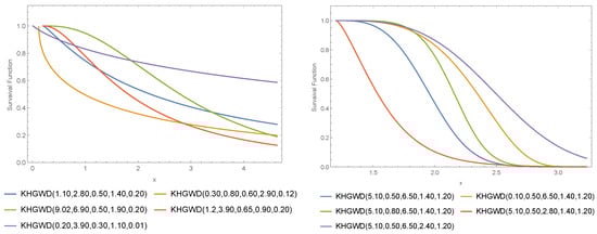
Figure 1. Different SF for the $\mathrm{KHGWD}(\alpha ,\beta ,\lambda ,\mu ,\nu )$.

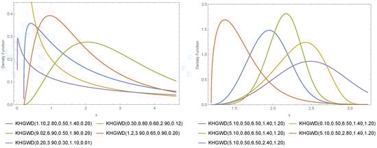
Figure 2. Different PDF for the $\mathrm{KHGWD}(\alpha ,\beta ,\lambda ,\mu ,\nu )$.

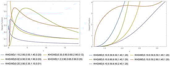
Figure 3. Different HRF for the $\mathrm{KHGWD}(\alpha ,\beta ,\lambda ,\mu ,\nu )$.

The model is sometimes very flexible. It seems to approach the bell curve with some torsion, as seen in the right panel of Figure 2. At other times, it seems to have strong tails, as seen in the left panel of Figure 2, which depends on the particular values of the parameters. The left panel of Figure 2 also shows that the proposed model has heavy tails when the parameters are increased. Based on the behavior of the proposed model shown in Figure 2, it is a good candidate for modeling semi-normal data (right part) and data with heavy tails (left part) in various financial, industrial, medical, and global epidemiological applications which have the same behavior. However, from the plots in Figure 3, it is clear that the KHGWD has unimodal and increasing failure rate functions. The unimodal and increasing failure rate functions are another superiority of the proposed model along with the heavy-tailed behavior. Therefore, the proposed model is suitable for modeling COVID-19.

3. Mathematical Properties

This section is devoted to deriving some mathematical properties of the $\mathrm{KHGWD}(\alpha ,\beta ,\lambda ,\mu ,\nu )$.

3.1. Quantile Function

To generate random variables by Monte Carlo simulation, the quantile function of the distribution is required. Assuming $p\sim Uniform(0,1)$, we solved the following equation for the quantile function $\Lambda \left(p\right)$:

$$\begin{array}{c}\hfill p=\frac{1-e^{-\alpha {\left(F(\Lambda \left(p\right))\right)}^{\beta }}}{1-e^{-\alpha }}.\end{array}$$

(10)

Letting $y=F(\Lambda (p\left)\right)$, we have

$$\begin{array}{c}\hfill p=\frac{1-e^{-\alpha {\left(y\right)}^{\beta }}}{1-e^{-\alpha }}.\end{array}$$

(11)

By solving for y, we have

$$\begin{array}{c}\hfill F(\Lambda \left(p\right))={\left(-\frac{log\left[1-p\left(1-e^{-\alpha }\right)\right]}{\alpha }\right)}^{\frac{1}{\beta }}.\end{array}$$

(12)

Thus,

$$\begin{array}{c}\hfill \Lambda \left(p\right)=F^{-1}\{{\left(-\frac{log\left[1-p\left(1-e^{-\alpha }\right)\right]}{\alpha }\right)}^{\frac{1}{\beta }}\},\end{array}$$

(13)

where $F^{-1}$ is the quantile of the baseline distribution $\mathrm{KHGWD}(\alpha ,\beta ,\lambda ,\mu ,\nu )$. Inverting $F\left(x\right)=p$ in (6), we can write

$$\begin{array}{c}\hfill {\Lambda }_{\mathrm{KHGWD}}(x,\alpha ,\beta ,\lambda ,\mu ,\nu )=\nu +\mu {\left(-log\left[1-{\left(-\frac{log\left[1-\left(1-e^{-\alpha }\right)x\right]}{\alpha }\right)}^{\frac{1}{\beta }}\right]\right)}^{\frac{1}{\lambda }}.\end{array}$$

(14)

By setting x as a uniform R.V. in the unit interval (0, 1), we can also use (14) for simulating $\mathrm{KHGWD}(\alpha ,\beta ,\lambda ,\mu ,\nu )$ R.V.s. Figure 4 plots different quantile functions for the $\mathrm{KHGWD}(\alpha ,\beta ,\lambda ,\mu ,\nu )$, and particularly for (1) $\beta =2.3;\lambda =0.2,\mu =0.2,\nu =3.2.$ (2) $\alpha =4.3$, $\lambda =0.2,\mu =0.2,\nu =3.2.$ (3) $\alpha =4.3,\beta =0.3,\mu =0.2,\nu =3.2$. (4) $\alpha =4.3,\beta =0.3,$$\lambda =0.2,\nu =3.2.$ (5) $\alpha =0.3,\beta =0.3,\lambda =1.2,\mu =0.2$, respectively. Some numerical values of the quantile measure are provided in Table 1.

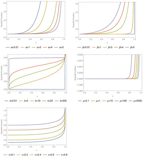
Figure 4. Different quantile functions for the $\mathrm{KHGWD}(\alpha ,\beta ,\lambda ,\mu ,\nu )$.

Table 1. Some quantile values for $\alpha =1.3,\beta =5.3,\lambda =0.2,\mu =0.2,$ and $\nu =3.2$.

x	$\mathbf{\Lambda }\left(\mathit{x}\right)$
0.1	3.30459
0.2	3.54091
0.3	3.97569
0.4	4.74677
0.5	6.13344
0.6	8.75958
0.7	14.2517
0.8	28.0657
0.9	80.4795

In addition, the effects of shape parameters on skewness and kurtosis can be determined using quantile measures. We obtain skewness and kurtosis measures of $\mathrm{KHGWD}(\alpha ,\beta ,\lambda ,\mu ,\nu )$. The skewness (SK) (see Bowley [8]) of X is given by

$$\mathrm{SK}(\alpha ,\beta ,\lambda ,\mu ,\nu )=\frac{2\Lambda \left(1/2\right)-\Lambda \left(3/4\right)-\Lambda \left(1/4\right)}{\Lambda \left(1/4\right)-\Lambda \left(3/4\right)},$$

and the Kurtosis (K) (see Moor [9]) is given by

$$\mathrm{K}(\alpha ,\beta ,\lambda ,\mu ,\nu )=\frac{\Lambda \left(1/8\right)-\Lambda \left(3/8\right)+\Lambda \left(5/8\right)-\Lambda \left(7/8\right)}{\Lambda \left(2/8\right)-\Lambda \left(6/8\right)}.$$

Figure 5 shows $\mathrm{SK}(\alpha ,\beta ,0.2,0.2,3.2)$ and $\mathrm{K}(\alpha ,\beta ,0.2,0.2,3.2)$ for different values of $\alpha$ and $\beta$. Figure 6, on the other hand, shows $\mathrm{SK}(1.3,5.3,\lambda ,\mu ,3.2)$ and $\mathrm{K}(1.3,5.3,$$\lambda ,\mu ,3.2)$ for different values of $\lambda$ and $\mu$.

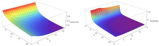
Figure 5. Plots for the $\mathrm{SK}(\alpha ,\beta ,0.2,0.2,3.2)$ and $\mathrm{K}(\alpha ,\beta ,0.2,0.2,3.2)$.

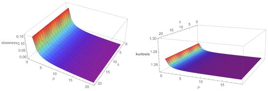
Figure 6. Plots for the $\mathrm{SK}(1.3,5.3,\lambda ,\mu ,3.2)$ and $\mathrm{K}(1.3,5.3,\lambda ,\mu ,3.2)$.

3.2. The Expansion for KHGWD Density Function

Using the general binomial and the power series expansion, we have

$$\begin{array}{ccc}\hfill {\left(1-e^{-{\left(\frac{x-\nu }{\mu }\right)}^{\lambda }}\right)}^{\beta -1}& =& \sum _{\kappa =0}^{\infty }\left(\genfrac{}{}{0pt}{}{\beta -1}{\kappa }\right){(-1)}^{\kappa }{e}^{-\kappa {\left(\frac{x-\nu }{\mu }\right)}^{\lambda }}\hfill \\ & =& \sum _{\kappa =0}^{\infty }\left(\genfrac{}{}{0pt}{}{\beta -1}{\kappa }\right){(-1)}^{\kappa }\sum _{h=0}^{\infty }\frac{{(-1)}^h}{h!}{\left(\frac{x-\nu }{\mu }\right)}^{\lambda h}.\hfill \end{array}$$

(15)

Next, we can also write

$$\begin{array}{ccc}\hfill & & e^{-{\left(\frac{x-\nu }{\mu }\right)}^{\lambda }-\alpha {\left(1-e^{-{\left(\frac{x-\nu }{\mu }\right)}^{\lambda }}\right)}^{\beta }}\hfill \\ & & =\sum _{\rho =0}^{\infty }\frac{{(-1)}^{\rho }}{\rho !}{\left({\left(\frac{x-\nu }{\mu }\right)}^{\lambda }+\alpha {\left(1-e^{-{\left(\frac{x-\nu }{\mu }\right)}^{\lambda }}\right)}^{\beta }\right)}^{\rho }\hfill \\ & & =\sum _{\rho =0}^{\infty }\frac{{(-1)}^{\rho }}{\rho !}\sum _{q=0}^{\infty }\left(\genfrac{}{}{0pt}{}{\rho }{q}\right){\left(\frac{x-\nu }{\mu }\right)}^{\lambda q}{\alpha }^{\rho -q}{\left(1-e^{-{\left(\frac{x-\nu }{\mu }\right)}^{\lambda }}\right)}^{\beta (\rho -q)},\hfill \end{array}$$

(16)

Using (15) and (16), the PDF of the expanded $\mathrm{KHGWD}(\alpha ,\beta ,\lambda ,\mu ,\nu )$ is given by

$$\begin{array}{ccc}\hfill f(x;\alpha ,\beta ,\lambda ,\mu ,\nu )& =& \frac{\alpha \beta \lambda }{\mu \left(1-e^{-\alpha }\right)}\sum _{\kappa =0}^{\infty }\left(\genfrac{}{}{0pt}{}{\beta -1}{\kappa }\right)\sum _{h=0}^{\infty }\sum _{\rho =0}^{\infty }\sum _{q=0}^{\infty }{\alpha }^{\rho -q}\hfill \\ & \times & \sum _{\tau =0}^{\infty }\sum _{\delta =0}^{\infty }{\Psi }_{\kappa ,h,\rho ,q,\tau ,\delta }{\left(\frac{x-\nu }{\mu }\right)}^{\lambda (h+q+\delta +1)-1},\hfill \end{array}$$

(17)

where

$${\Psi }_{\kappa ,h,\rho ,q,\tau ,\delta }=\left(\genfrac{}{}{0pt}{}{\rho }{q}\right)\left(\genfrac{}{}{0pt}{}{\beta (\rho -q)}{\tau }\right)\frac{{(-1)}^{\kappa +h+\rho +\tau +\delta }{\tau }^{\delta }}{h!\rho !\delta !}.$$

3.3. The Expansion for the KHGWD Distribution Function

The CDF (15) of the expanded $\mathrm{KHGWD}(\alpha ,\beta ,\lambda ,\mu ,\nu )$ can be written as

$$\begin{array}{ccc}\hfill F(x;\alpha ,\beta ,\lambda ,\mu ,\nu )& =& \left(1-\sum _{h=0}^{\infty }\frac{{(-1)}^h}{h!}{\alpha }^h{\left(1-e^{-{\left(\frac{x-\nu }{\mu }\right)}^{\lambda }}\right)}^{h\beta }\right){\left(1-e^{-\alpha }\right)}^{-1}\hfill \\ & =& \left(1-\sum _{h=0}^{\infty }{\alpha }^h\sum _{\tau =0}^{\infty }\left(\genfrac{}{}{0pt}{}{h\beta }{\tau }\right)\sum _{\rho =0}^{\infty }{\Psi }_{h,\tau ,\rho }{\left(\frac{x-\nu }{\mu }\right)}^{\lambda \rho }\right){\left(1-e^{-\alpha }\right)}^{-1},\hfill \end{array}$$

(18)

where

$${\Psi }_{h,\tau ,\rho }=\frac{{(-1)}^{h+\tau +\rho }{\tau }^{\rho }}{h!\rho !}.$$

4. Estimation of the Parameters Based on the Ranked Set Samples

Let $\{X_{j,i},i=1,\dots ,m,j=1,\dots ,r\}$ be the observed sample, where $X_{j,i}$ is the ith order statistic in the jth group. The likelihood function based on the $\mathrm{KHGWD}(\alpha ,\beta ,\lambda ,\mu ,\nu )$, is given by

$$\begin{array}{c}\hfill l={\left(\frac{m!\alpha \beta }{1-e^{-\alpha }}\right)}^{rm}\prod _{j=1}^r\prod _{i=1}^m\frac{e^{-\alpha G_{j,i}^{\beta }}{\left(\frac{e^{-\alpha G_{j,i}^{\beta }}-1}{e^{-\alpha }-1}\right)}^{i-1}{\left(1-\frac{e^{-\alpha G_{j,i}^{\beta }}-1}{e^{-\alpha }-1}\right)}^{m-i}{g}_{j,i}{G}_{j,i}^{\beta -1}}{(i-1)!(m-i)!},\end{array}$$

(19)

where $G_{j,i}=G_{j,i}(x_{j,i},\lambda ,\mu ,\nu )$ and $g_{j,i}=g_{j,i}(x_{j,i},\lambda ,\mu ,\nu )$ are the baseline CDF (6) and PDF (7), respectively. The corresponding log-likelihood function is given by

$$\begin{array}{ccc}\hfill L& =& K_1+rmlog\left[\alpha \beta \right]-nlog\left[1-e^{-\alpha }\right]-\sum _{j=1}^r\sum _{i=1}^m\alpha G_{j,i}^{\beta }\hfill \\ & +& \sum _{j=1}^r\sum _{i=1}^m(i-1)log\left[\frac{e^{-\alpha G_{j,i}^{\beta }}-1}{e^{-\alpha }-1}\right]+(m-i)log\left[1-\frac{e^{-\alpha G_{j,i}^{\beta }}-1}{e^{-\alpha }-1}\right]\hfill \\ & +& \sum _{j=1}^r\sum _{i=1}^{m}log\left[g_{j,i}\right]+(\beta -1)log\left[G_{j,i}\right],\hfill \end{array}$$

(20)

where $K_1$ is constant. The first partial derivatives of log-likelihood (20) with respect to $\alpha ,\beta ,\lambda ,\mu ,\nu$, respectively, are given by

$$\begin{array}{ccc}\frac{\partial L}{\partial \alpha }& =& n\left(\frac{1}{\alpha }-\frac{e^{-\alpha }}{1-e^{-\alpha }}\right)-\sum _{j=1}^r\sum _{i=1}^m{G}_{j,i}^{\beta }\hfill \\ & +& \sum _{j=1}^r\sum _{i=1}^m\left(\frac{(i-1)}{e^{-\alpha G_{j,i}^{\beta }}-1}-\frac{(m-i)}{e^{-\alpha }-e^{-\alpha G_{j,i}^{\beta }}}\right)\left(\frac{e^{-\alpha }\left(e^{-\alpha G_{j,i}^{\beta }}-1\right)}{\left(e^{-\alpha }-1\right)}-e^{-\alpha G_{j,i}^{\beta }}{G}_{j,i}^{\beta }\right),\hfill \end{array}$$

(21)

$$\begin{array}{ccc}\hfill \frac{\partial L}{\partial \beta }& =& \frac{n}{\beta }\hfill \\ & +& \alpha \sum _{j=1}^r\sum _{i=1}^m{G}_{j,i}^{\beta }\left(1-log\left[G_{j,i}\right]\left(1+\left(\frac{m-i}{e^{-\alpha }-e^{-\alpha G_{j,i}^{\beta }}}-\frac{i-1}{e^{-\alpha G_{j,i}^{\beta }}-1}\right)e^{-\alpha G_{j,i}^{\beta }}\right)\right),\hfill \end{array}$$

(22)

$$\begin{array}{ccc}\hfill \frac{\partial L}{\partial \lambda }& =& \sum _{j=1}^r\sum _{i=1}^m\frac{g_{j,i}^{\left(\lambda \right)}}{g_{j,i}}+G_{j,i}^{\left(\lambda \right)}\left(\frac{\beta -1}{G_{j,i}}-\alpha \beta G_{j,i}^{\beta -1}\right)\hfill \\ & -& \alpha \beta \sum _{j=1}^r\sum _{i=1}^m{G}_{j,i}^{\beta -1}{G}_{j,i}^{\left(\lambda \right)}{e}^{-\alpha G_{j,i}^{\beta }}\left(\frac{i-1}{e^{-\alpha G_{j,i}^{\beta }}-1}+\frac{m-i}{e^{-\alpha }-e^{-\alpha G_{j,i}^{\beta }}}\right),\hfill \end{array}$$

(23)

$$\begin{array}{ccc}\hfill \frac{\partial L}{\partial \mu }& =& \sum _{j=1}^r\sum _{i=1}^m\frac{g_{j,i}^{\left(\mu \right)}}{g_{j,i}}+G_{j,i}^{\left(\mu \right)}\left(\frac{\beta -1}{G_{j,i}}-\alpha \beta G_{j,i}^{\beta -1}\right)\hfill \\ & -& \alpha \beta \sum _{j=1}^r\sum _{i=1}^m{G}_{j,i}^{\beta -1}{G}_{j,i}^{\left(\mu \right)}{e}^{-\alpha G_{j,i}^{\beta }}\left(\frac{i-1}{e^{-\alpha G_{j,i}^{\beta }}-1}+\frac{m-i}{e^{-\alpha }-e^{-\alpha G_{j,i}^{\beta }}}\right),\hfill \end{array}$$

(24)

and

$$\begin{array}{ccc}\hfill \frac{\partial L}{\partial \nu }& =& \sum _{j=1}^r\sum _{i=1}^m\frac{g_{j,i}^{\left(\nu \right)}}{g_{j,i}}+G_{j,i}^{\left(\nu \right)}\left(\frac{\beta -1}{G_{j,i}}-\alpha \beta G_{j,i}^{\beta -1}\right)\hfill \\ & -& \alpha \beta \sum _{j=1}^r\sum _{i=1}^m{G}_{j,i}^{\beta -1}{G}_{j,i}^{\left(\nu \right)}{e}^{-\alpha G_{j,i}^{\beta }}\left(\frac{i-1}{e^{-\alpha G_{j,i}^{\beta }}-1}+\frac{m-i}{e^{-\alpha }-e^{-\alpha G_{j,i}^{\beta }}}\right),\hfill \end{array}$$

(25)

where

$$\begin{array}{ccc}\hfill G_{j,i}^{\left(\lambda \right)}& =& \frac{\partial G_{j,i}}{\partial \lambda }={\left(\frac{x_{j,i}-\nu }{\mu }\right)}^{\lambda }{e}^{-{\left(\frac{x_{j,i}-\nu }{\mu }\right)}^{\lambda }}log\left[\frac{x_{j,i}-\nu }{\mu }\right],\hfill \end{array}$$

(26)

$$\begin{array}{ccc}\hfill G_{j,i}^{\left(\mu \right)}& =& \frac{\partial G_{j,i}}{\partial \mu }=-\frac{\lambda }{\mu }{\left(\frac{x_{j,i}-\nu }{\mu }\right)}^{\lambda }{e}^{-{\left(\frac{x_{j,i}-\nu }{\mu }\right)}^{\lambda }},\hfill \end{array}$$

(27)

$$\begin{array}{ccc}\hfill G_{j,i}^{\left(\nu \right)}& =& \frac{\partial G_{j,i}}{\partial \nu }=-\frac{\lambda }{\mu }{\left(\frac{x_{j,i}-\nu }{\mu }\right)}^{\lambda -1}{e}^{-{\left(\frac{x_{j,i}-\nu }{\mu }\right)}^{\lambda }},\hfill \end{array}$$

(28)

$$\begin{array}{ccc}\hfill g_{j,i}^{\left(\lambda \right)}& =& \frac{\partial g_{j,i}}{\partial \lambda }=\mu {\left(\frac{x_{j,i}-\nu }{\mu }\right)}^{\lambda -1}\left(-1+\lambda log\left[\frac{x_{j,i}-\nu }{\mu }\right]\left({\left(\frac{x_{j,i}-\nu }{\mu }\right)}^{\lambda }-1\right)\right)e^{-{\left(\frac{x_{j,i}-\nu }{\mu }\right)}^{\lambda }},\hfill \end{array}$$

(29)

$$\begin{array}{ccc}\hfill g_{j,i}^{\left(\mu \right)}& =& \frac{\partial g_{j,i}}{\partial \mu }=-{\left(\frac{\lambda }{\mu }\right)}^2{\left(\frac{x_{j,i}-\nu }{\mu }\right)}^{\lambda -1}\left({\left(\frac{x_{j,i}-\nu }{\mu }\right)}^{\lambda }-1\right)e^{-{\left(\frac{x_{j,i}-\nu }{\mu }\right)}^{\lambda }},\hfill \end{array}$$

(30)

and

$$\begin{array}{ccc}\hfill g_{j,i}^{\left(\nu \right)}& =& \frac{\partial g_{j,i}}{\partial \nu }=\lambda {\mu }^2{\left(\frac{x_{j,i}-\nu }{\mu }\right)}^{\lambda -2}\left(1+\lambda \left({\left(\frac{x_{j,i}-\nu }{\mu }\right)}^{\lambda }-1\right)\right)e^{-{\left(\frac{x_{j,i}-\nu }{\mu }\right)}^{\lambda }}.\hfill \end{array}$$

(31)

The maximum likelihood estimators ${\widehat{\alpha }}_{ML},{\widehat{\beta }}_{ML},{\widehat{\lambda }}_{ML},{\widehat{\mu }}_{ML},$ and ${\widehat{\nu }}_{ML}$ of the KHGWD parameters are the solutions of the nonlinear Equations (21)–(25) for $r=m=n$. Characteristically, they can be solved by fixed-point iteration methods or the Newtonian approach.

5. Monte Carlo Simulation Study

This section is concerned with evaluating the performance of the maximum likelihood estimators of $\mathrm{KHGWD}(\alpha ,\beta ,\lambda ,\mu ,\nu )$ through a Monte Carlo simulation study. The R program through the optimum function can used to compute the simulation and application results. The Weibull location parameter $\nu$ was set to zero to simplify the calculations.

The simulation of the KHGWD model is performed for two parameter sets:

• Set 1: $\alpha =3.2,\beta =1.5,\lambda =3.8,\mu =2.1,\nu =0.$
• Set 2: $\alpha =4.3,\beta =1.6,\lambda =3.5,\mu =1.8,\nu =0.$

The simulation study is performed as follows.

• Random samples of sizes $n=25,100,225,400,625,900$ are generated from KHGWD and are randomly divided into r groups of equal size m, where $r=m=5,10,15,20,25,$ and 30, respectively.
• The model parameters have been estimated via the maximum likelihood method.
• Five-thousand repetitions are made to calculate these estimators’ biases, absolute biases, and mean square errors (MSEs).
• The formulas for obtaining the estimate, biases, and MSEs are given respectively, by

  $$\widehat{\alpha }=\frac{1}{5000}\sum _{i=1}^{5000}{\widehat{\alpha }}_i,$$

  $$\mathrm{Bias}\left(\widehat{\alpha }\right)=\frac{1}{5000}\sum _{i=1}^{5000}\left({\widehat{\alpha }}_i-\alpha \right),$$

  and

  $$\mathrm{MSE}\left(\widehat{\alpha }\right)=\frac{1}{5000}\sum _{i=1}^{5000}{\left({\widehat{\alpha }}_i-\alpha \right)}^2,$$

  respectively.
• Step (4) is also repeated for the parameters $\beta ,\lambda ,$ and $\mu$.

The simulation results of the KHGWD for Set 1 and Set 2 are presented in Table 2 and Table 3, respectively. Figure 7 and Figure 8 displays graphically the results provided in Table 2 and Table 3, respectively.

Table 2. Simulation results of the KHGWD for Set 1.

n	$\widehat{\mathit{\alpha }}$	$\widehat{\mathit{\beta }}$	$\widehat{\mathit{\lambda }}$	$\widehat{\mathit{\mu }}$
	2.07	2.551	4.044	1.805
25	4.087	4.598	2.946	0.255
	−1.13	1.051	0.244	−0.295
	2.586	2.104	3.787	1.917
100	3.3	2.076	1.692	0.165
	−0.614	0.604	−0.013	−0.183
	2.838	1.9	3.675	1.973
225	2.949	1.01	1.019	0.12
	−0.361	0.4	−0.124	−0.127
	2.988	1.792	3.645	2.007
400	2.523	0.54	0.681	0.089
	−0.212	0.292	−0.155	−0.093
	3.053	1.722	3.645	2.028
625	2.199	0.317	0.469	0.069
	−0.147	0.222	−0.155	−0.072
	3.115	1.702	3.64	2.04
900	2.053	0.271	0.397	0.061
	−0.085	0.202	−0.16	−0.06

The first, second, and third rows represent the estimate, MSE, and Bias, respectively.

Table 3. Simulation results of the KHGWD for Set 2.

n	$\widehat{\mathit{\alpha }}$	$\widehat{\mathit{\beta }}$	$\widehat{\mathit{\lambda }}$	$\widehat{\mathit{\mu }}$
	3.476	2.514	4.396	1.609
25	6.169	4.551	5.554	0.26
	−0.824	0.914	0.895	−0.1907
	3.182	2.182	3.799	1.606
100	4.908	2.272	2.602	0.155
	−1.118	0.582	0.299	−0.194
	3.511	1.941	3.614	1.663
225	3.812	1.072	1.324	0.095
	−0.789	0.341	0.114	−0.137
	3.712	1.844	3.512	1.693
400	3.257	0.578	0.768	0.066
	−0.588	0.244	0.012	−0.107
	3.883	1.799	3.453	1.716
625	2.644	0.361	0.471	0.047
	−0.417	0.199	−0.047	−0.084
	4.054	1.765	3.443	1.737
900	2.274	0.27	0.386	0.035
	−0.246	0.165	−0.057	−0.063

The first, second, and third rows represent the estimate, MSE, and Bias, respectively.

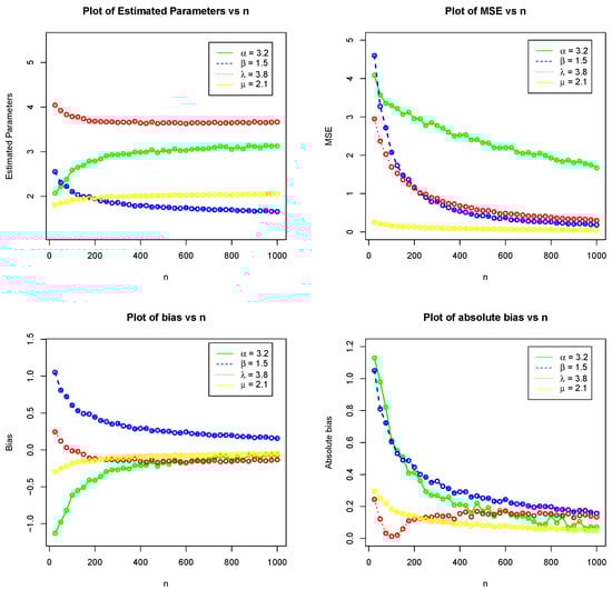
Figure 7. Plot of the simulation results of the KHGWD for Set 1.

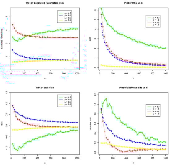
Figure 8. Plot of the simulation results of the KHGWD for Set 2.

Figure 7 and Figure 8 illustrate the simulation results for the above measures. These plots show that increasing the sample size n leads to a reduction in the estimated biases. In addition, increasing the sample size n leads to a decrease in the estimated MSEs, which approaches zero as n increases. These results demonstrate both the efficiency and consistency properties of the MLEs.

6. COVID-19 Data

The COVID-19 dataset of Hong and Li [10] is considered an application of the KHGWD model and is randomly divided into seven groups of similar seven observations. Table 4 shows the descriptive statistics of the proposed COVID-19 data. The boxplot and Q-Q plot are shown in Figure 9. By performing the maximum likelihood estimators of $\mathrm{KHGWD}(\alpha ,\beta ,\lambda ,\mu ,\nu )$ by Monte Carlo simulation study for $\nu =0$, the estimated parameters are $\widehat{\alpha }=2.4222994$, $\widehat{\beta }=0.1311977,\widehat{\lambda }=5.3593414$, and $\widehat{\mu }=20.1015298$. Figure 10: Plots of the fitted PDF of KHGWD and CDF. Figure 11: PP plot and Kaplan–Meier survival function of KHGWD.

Table 4. Descriptive statistics of the COVID-19 data.

Min.	1st Qu.	Median	Mean	3rd Qu.	Max
0.054	0.704	3.079	4.787	6.743	20.083

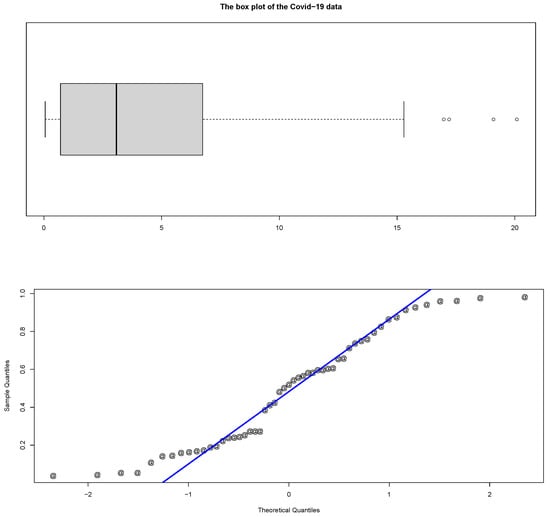
Figure 9. The boxplot and Q-Q plot of the COVID-19 data.

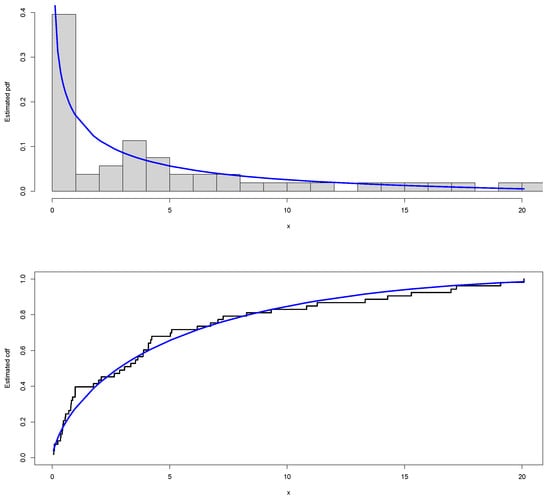
Figure 10. The fitted PDF and CDF of the KHGWD.

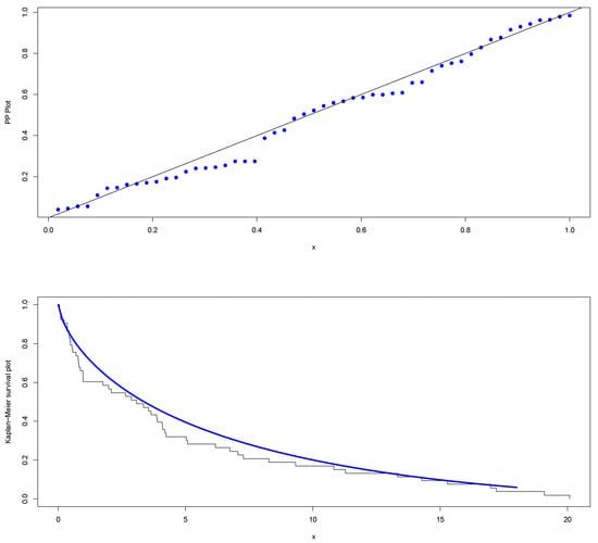
Figure 11. The PP plot and the Kaplan–Meier survival function of the KHGWD.

Table 5 compares the KHGWD based on one-sample Kolmogorov–Smirnov test. The goodness-of-fit results of the KHGWD model are compared with some other models, including the Khalil generalized exponential distribution (KHGEXP), the Khalil generalized gamma distribution (KHGGamma), and Weibull distribution. The distribution functions of these competitive distributions are given by

Table 5. Relative quality of the KHGWD vs. competing models.

Model	p-Value
KHGWD	0.4347
KHGEXP	0.3776
KHGGamma	0.4056
Weibull	0.3776

(1) KHGEXP distribution:

$$\begin{array}{c}\hfill F(x;\alpha ,\beta ,\mu )=\frac{1-e^{-\alpha {\left(1-e^{-\left(\frac{x}{\mu }\right)}\right)}^{\beta }}}{1-e^{-\alpha }},x\ge 0,\alpha ,\beta ,\mu >0.\end{array}$$

(32)

(2) KHGGamma distribution:

$$\begin{array}{c}\hfill F(x;\alpha ,\beta ,\lambda ,\mu )=\frac{e^{-\alpha {\left(\frac{1}{\Gamma \lambda }\gamma (\lambda ,\mu x)\right)}^{\beta }}-1}{e^{-\alpha }-1},x\ge 0,\alpha ,\beta ,\lambda ,\mu >0,\end{array}$$

(33)

where $\gamma (\lambda ,\mu x)$ is the lower incomplete gamma function.

(3) Weibull distribution:

$$\begin{array}{c}\hfill F(x;\lambda ,\mu )=1-e^{-{\left(\frac{x}{\mu }\right)}^{\lambda }},x\ge 0;\lambda ,\mu >0.\end{array}$$

(34)

Based on the results presented in Table 5, we see that KHGWD is a good competitor among the competing models for modeling the COVID-19 data.

7. Conclusions

We introduced the new generalized Weibull distribution of Khalil with five parameters. The model has a high degree of flexibility to fit the appropriate data. The model is unimodal, has a strong tail-heavy behavior, and exhibits increasing failure rate functions. We have studied some mathematical and statistical functions and the effects of shape parameters on skewness and kurtosis. We have provided density and distribution functions in an extended form. Based on ranked samples, the maximum likelihood estimators for the intended model parameters and a Monte Carlo simulation study are provided. A COVID-19 dataset is analyzed to illustrate the applicability and potential of the intended distribution. The biases and mean square errors decrease as the sample size increases. It is clear that the proposed model fits the estimated PDF and CDF plots well. The COVID-19 dataset has a strong deflection that is skewed to the right in the boxplot. The proposed model fits the Kaplan–Meier survival plot very well. The new generalized Weibull distribution of Khalil, based on the Kolmogorov–Smirnov one-sample test, provides a better fit than other competing models. The results show that the model is considered ideal for modeling COVID-19.

References

- McIntyre, G.A. A method for unbiased selective sampling, using ranked sets. Aust. J. Agric. Res. 1952, 3, 385–390. [Google Scholar] [CrossRef]
- Frey, J. A note on Fisher information and imperfect ranked-set sampling. Commun. Stat.-Theory Methods 2014, 43, 2726–2733. [Google Scholar] [CrossRef]
- Park, S.; Lim, J. On the effect of imperfect ranking on the amount of Fisher information in ranked set samples. Commun. Stat.-Theory Methods 2012, 413, 3608–3620. [Google Scholar] [CrossRef]
- Chen, Z.; Bai, Z.; Sinha, B. Ranked Set Sampling: Theory and Applications; Springer: New York, NY, USA, 2013. [Google Scholar]
- Tahmasebi, S.; Longobardi, M.; Kazemi, M.R.; Alizadeh, M. Cumulative Tsallis entropy for maximum ranked set sampling with unequal samples. Phys. A Stat. Mech. Appl. 2020, 556, 124763. [Google Scholar] [CrossRef]
- Arnold, B.C.; Balakrishnan, N.; Nagaraja, H.N. A First Course in Order Statistics; John Wiley & Sons: New York, NY, USA, 1992. [Google Scholar]
- Najma, S.; Alamgir, K.; Wali, K.; Habib, S.; Pijitra, J.; Thammarat, P. A Novel Generalized Family of Distributions for Engineering and Life Sciences Data Applications. Math. Probl. Eng. 2021, 2021, 9949999. [Google Scholar]
- Bowley, A.L. Elements of Statistics, 4th ed.; Charles Scribner’s Sons: New York, NY, USA, 1920. [Google Scholar]
- Moors, J.J.A. The meaning of kurtosis: Darlington re-examined. Am. Stat. 1986, 40, 283–284. [Google Scholar]
- Hong, H.G.; Li, Y. Estimation of time-varying reproduction numbers underlying epidemiological processes: A new statistical tool for the COVID-19 pandemic. PLoS ONE 2020, 15, e0236464. [Google Scholar] [CrossRef] [PubMed]
Publisher’s Note: MDPI stays neutral with regard to jurisdictional claims in published maps and institutional affiliations. |
© 2022 by the authors. Licensee MDPI, Basel, Switzerland. This article is an open access article distributed under the terms and conditions of the Creative Commons Attribution (CC BY) license (https://creativecommons.org/licenses/by/4.0/).