
Perceptual Hash of Neural Networks


Abstract
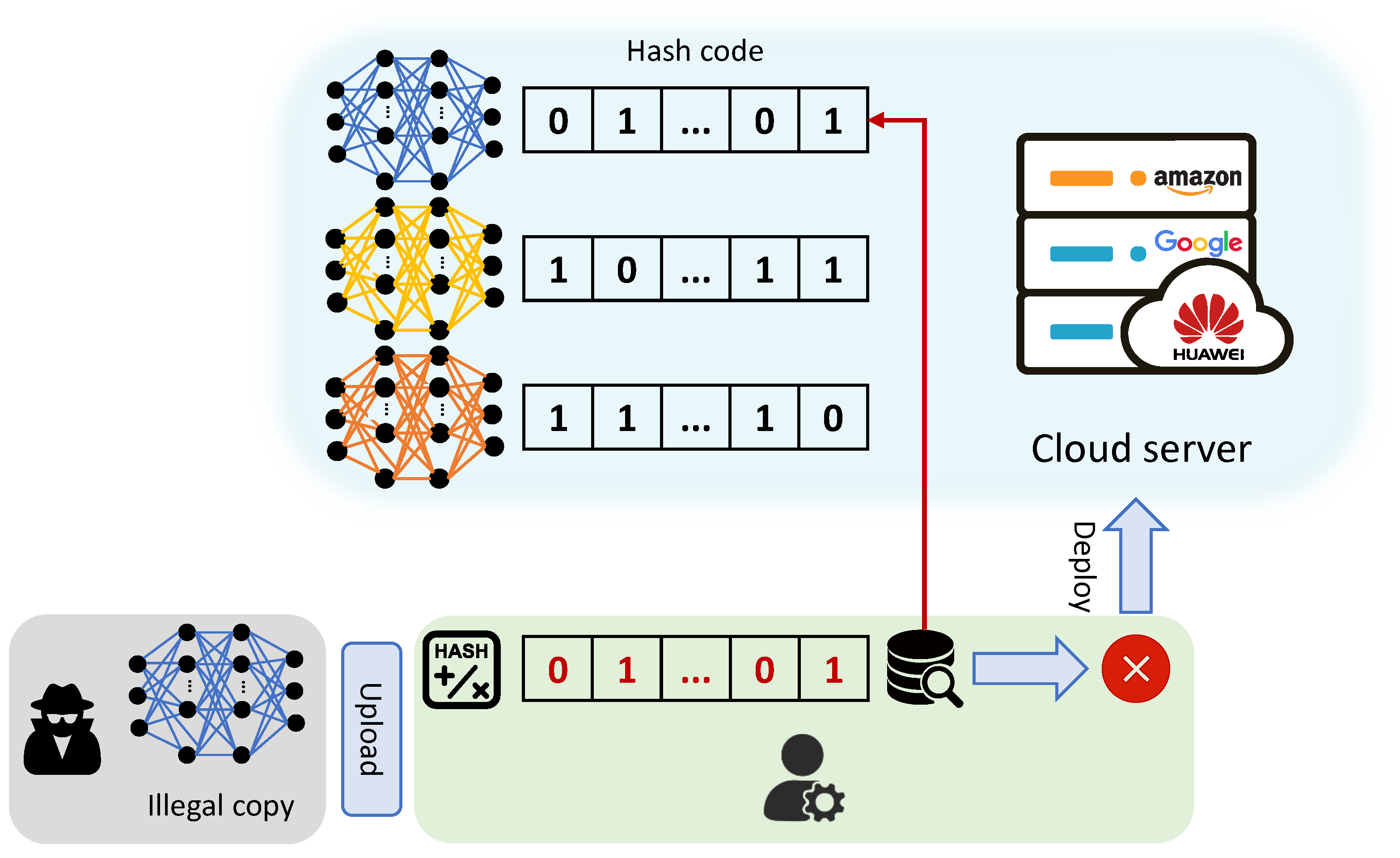
:1. Introduction
- We propose a new idea of generating perceptual hash for neural networks, which can be used in model protection;
- The proposed deep hashing scheme based on neural graph work is capable of all kinds of deep learning frameworks;
- The proposed method is effective that has a good retrieval performance.
2. Related Works
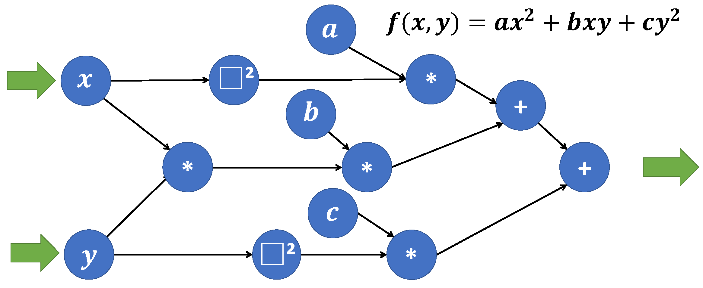
2.1. Computational Graph
2.2. Deep Image Hashing
2.3. Graph Hashing
3. Deep Neural Network Hashing
3.1. Problem Definition
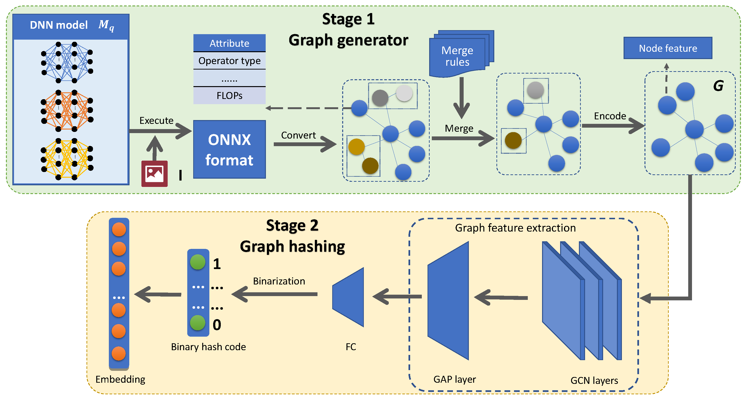
3.2. Stage 1: Graph Generator
3.2.1. ONNX Operation
3.2.2. Merge Operation
3.2.3. Node Feature Embedding
3.3. Stage 2: Graph Hashing
3.4. Objective Loss Function
4. Experiments
4.1. Implementation Details
4.1.1. Network Architecture
4.1.2. Training Parameters
4.1.3. Dataset
4.1.4. Evaluation Metrics
4.2. Comparison with State-of-the-Art Methods
4.2.1. Methods in Comparison
4.2.2. Results
4.3. Ablation Analysis
4.3.1. The Role of Merge Operation
4.3.2. Effect of the Classification Loss and the Quantization Loss
5. Conclusions
Author Contributions
Funding
Institutional Review Board Statement
Informed Consent Statement
Data Availability Statement
Acknowledgments
Conflicts of Interest
References
- LeCun, Y.; Bengio, Y.; Hinton, G. Deep learning. Nature 2015, 521, 436–444. [Google Scholar] [CrossRef] [PubMed]
- Goodfellow, I.; Bengio, Y.; Courville, A. Deep Learning; MIT Press: Cambridge, MA, USA, 2016. [Google Scholar]
- Voulodimos, A.; Doulamis, N.; Doulamis, A.; Protopapadakis, E. Deep learning for computer vision: A brief review. Comput. Intell. Neurosci. 2018, 2018, 7068349. [Google Scholar] [CrossRef] [PubMed]
- Hemanth, D.J.; Estrela, V.V. Deep Learning for Image Processing Applications; IOS Press: Amsterdam, The Netherlands, 2017; Volume 31. [Google Scholar]
- Young, T.; Hazarika, D.; Poria, S.; Cambria, E. Recent trends in deep learning based natural language processing. IEEE Comput. Intell. Mag. 2018, 13, 55–75. [Google Scholar] [CrossRef]
- Purwins, H.; Li, B.; Virtanen, T.; Schlüter, J.; Chang, S.Y.; Sainath, T. Deep learning for audio signal processing. IEEE J. Sel. Top. Signal Process. 2019, 13, 206–219. [Google Scholar] [CrossRef] [Green Version]
- Lee, H.; Pham, P.; Largman, Y.; Ng, A. Unsupervised feature learning for audio classification using convolutional deep belief networks. Adv. Neural Inf. Process. Syst. 2009, 22, 1096–1104. [Google Scholar]
- Sundararajan, K.; Woodard, D.L. Deep learning for biometrics: A survey. ACM Comput. Surv. 2018, 51, 1–34. [Google Scholar] [CrossRef]
- Hinton, G.; Vinyals, O.; Dean, J. Distilling the Knowledge in a Neural Network. Comput. Sci. 2015, 14, 38–39. [Google Scholar]
- Zhou, J.; Cui, G.; Zhang, Z.; Yang, C.; Liu, Z.; Wang, L.; Li, C.; Sun, M. Graph neural networks: A review of methods and applications. arXiv 2018, arXiv:1812.08434. [Google Scholar] [CrossRef]
- Kantorovich, L.V. On a mathematical symbolism convenient for performing machine calculations. Dokl. Akad. Nauk SSSR 1957, 113, 738–741. [Google Scholar]
- Bauer, F.L. Computational graphs and rounding error. SIAM J. Numer. Anal. 1974, 11, 87–96. [Google Scholar] [CrossRef]
- Xia, R.; Pan, Y.; Lai, H.; Liu, C.; Yan, S. Supervised Hashing for Image Retrieval via Image Representation Learning. In Proceedings of the AAAI Conference on Artificial Intelligence, Québec City, QC, Canada, 27–31 July 2014; Volume 28. [Google Scholar]
- Li, W.J.; Wang, S.; Kang, W.C. Feature learning based deep supervised hashing with pairwise labels. arXiv 2015, arXiv:1511.03855. [Google Scholar]
- Cao, Z.; Long, M.; Wang, J.; Yu, P.S. Hashnet: Deep learning to hash by continuation. In Proceedings of the IEEE International Conference on Computer Vision, Venice, Italy, 22–29 October 2017; pp. 5608–5617. [Google Scholar]
- Lai, H.; Pan, Y.; Liu, Y.; Yan, S. Simultaneous feature learning and hash coding with deep neural networks. In Proceedings of the IEEE Conference on Computer Vision and Pattern Recognition, Boston, MA, USA, 7–12 June 2015; pp. 3270–3278. [Google Scholar]
- Erin Liong, V.; Lu, J.; Wang, G.; Moulin, P.; Zhou, J. Deep hashing for compact binary codes learning. In Proceedings of the IEEE Conference on Computer Vision and Pattern Recognition, Boston, MA, USA, 7–12 June 2015; pp. 2475–2483. [Google Scholar]
- Yang, H.F.; Lin, K.; Chen, C.S. Supervised learning of semantics-preserving hash via deep convolutional neural networks. IEEE Trans. Pattern Anal. Mach. Intell. 2017, 40, 437–451. [Google Scholar] [CrossRef] [PubMed] [Green Version]
- Hamaguchi, T.; Oiwa, H.; Shimbo, M.; Matsumoto, Y. Knowledge Transfer for Out-of-Knowledge-Base Entities: A Graph Neural Network Approach. arXiv 2017, arXiv:1706.05674. [Google Scholar]
- Battaglia, P.W.; Pascanu, R.; Lai, M.; Rezende, D.; Kavukcuoglu, K. Interaction Networks for Learning about Objects, Relations and Physics; Curran Associates Inc.: Red Hook, NY, USA, 2016. [Google Scholar]
- Hamilton, W.L.; Ying, R.; Leskovec, J. Inductive Representation Learning on Large Graphs. arXiv 2017, arXiv:1706.02216. [Google Scholar]
- Kipf, T.N.; Welling, M. Semi-supervised classification with graph convolutional networks. arXiv 2016, arXiv:1609.02907. [Google Scholar]
- Lee, J.B.; Rossi, R.; Kong, X. Graph classification using structural attention. In Proceedings of the 24th ACM SIGKDD International Conference on Knowledge Discovery &Data Mining, London, UK, 19–23 August 2018; pp. 1666–1674. [Google Scholar]
- Thekumparampil, K.K.; Wang, C.; Oh, S.; Li, L.J. Attention-based graph neural network for semi-supervised learning. arXiv 2018, arXiv:1803.03735. [Google Scholar]
- Veličković, P.; Cucurull, G.; Casanova, A.; Romero, A.; Lio, P.; Bengio, Y. Graph attention networks. arXiv 2017, arXiv:1710.10903. [Google Scholar]
- Bai, Y.; Ding, H.; Qiao, Y.; Marinovic, A.; Gu, K.; Chen, T.; Sun, Y.; Wang, W. Unsupervised inductive graph-level representation learning via graph-graph proximity. arXiv 2019, arXiv:1904.01098. [Google Scholar]
- Li, Y.; Gu, C.; Dullien, T.; Vinyals, O.; Kohli, P. Graph matching networks for learning the similarity of graph structured objects. arXiv 2019, arXiv:1904.12787. [Google Scholar]
- Bai, Y.; Ding, H.; Bian, S.; Chen, T.; Sun, Y.; Wang, W. Simgnn: A neural network approach to fast graph similarity computation. In Proceedings of the Twelfth ACM International Conference on Web Search and Data Mining, Melbourne, Australia, 11–15 February 2019; pp. 384–392. [Google Scholar]
- Ying, Z.; You, J.; Morris, C.; Ren, X.; Hamilton, W.; Leskovec, J. Hierarchical graph representation learning with differentiable pooling. In Proceedings of the 32nd International Conference on Neural Information Processing Systems, Montreal, QC, Canada, 3–8 December 2018; pp. 4800–4810. [Google Scholar]
- Bai, Y.; Ding, H.; Gu, K.; Sun, Y.; Wang, W. Learning-Based Efficient Graph Similarity Computation via Multi-Scale Convolutional Set Matching. In Proceedings of the AAAI, New York, NY, USA, 7–12 February 2020; pp. 3219–3226. [Google Scholar]
- Qin, Z.; Bai, Y.; Sun, Y. GHashing: Semantic Graph Hashing for Approximate Similarity Search in Graph Databases. In Proceedings of the 26th ACM SIGKDD International Conference on Knowledge Discovery &Data Mining, Virtual Event, CA, USA, 6–10 July 2020; pp. 2062–2072. [Google Scholar]
- Paszke, A.; Gross, S.; Massa, F.; Lerer, A.; Bradbury, J.; Chanan, G.; Killeen, T.; Lin, Z.; Gimelshein, N.; Antiga, L.; et al. Pytorch: An imperative style, high-performance deep learning library. In Proceedings of the 33rd International Conference on Neural Information Processing Systems, Vancouver, BC, Canada, 8–14 December 2019; pp. 8026–8037. [Google Scholar]
- Onnx: Open Neural Network Exchange. 2019. Available online: https://github.com/onnx/onnx (accessed on 10 April 2022).
- Gao, X.; Xiao, B.; Tao, D.; Li, X. A survey of graph edit distance. Pattern Anal. Appl. 2010, 13, 113–129. [Google Scholar] [CrossRef]


| # | Category | Model Name in PyTorch |
|---|---|---|
| 1 | VGG | vgg 11, 13, 16 |
| 2 | Resnet | resnet 18, 34, 101 |
| 3 | mnaset | mnasnet 0_75, 1_0, 1_3 |
| 4 | DenseNet | densenet 121, 161, 201 |
| 5 | SqueezeNet | squeezenet 1_0, 1_1, v2_x0_5 |
| 6 | ShuffleNet | shufflenet v2_x0_5, v2_x1_5, v2_x2_0 |
| 7 | AlexNet | alexnet |
| 8 | Inception | inception_v3 |
| 9 | MobileNet | mobilenet_v2 |
| 10 | GoogLeNet | GoogLeNet |
| Methods | Metrics | Raw Data | Merged Data | ||||
|---|---|---|---|---|---|---|---|
| 16 Bits | 32 Bits | 64 Bits | 16 Bits | 32 Bits | 64 Bits | ||
| GHashing [31] | Recall | 0.559 | 0.565 | 0.707 | 0.559 | 0.74 | 0.719 |
| Precision | 0.67 | 0.692 | 0.828 | 0.758 | 0.889 | 0.861 | |
| score | 0.586 | 0.601 | 0.731 | 0.648 | 0.776 | 0.753 | |
| HNN-Net w/o | Recall | 0.519 | 0.522 | 0.677 | 0.648 | 0.721 | 0.727 |
| Precision | 0.675 | 0.624 | 0.83 | 0.805 | 0.88 | 0.867 | |
| score | 0.574 | 0.544 | 0.72 | 0.692 | 0.764 | 0.759 | |
| HNN-Net | Recall | 0.351 | 0.714 | 0.762 | 0.333 | 0.762 | 0.762 |
| Precision | 0.475 | 0.881 | 0.905 | 0.452 | 0.905 | 0.905 | |
| score | 0.4 | 0.762 | 0.794 | 0.375 | 0.794 | 0.794 | |
Publisher’s Note: MDPI stays neutral with regard to jurisdictional claims in published maps and institutional affiliations. |
© 2022 by the authors. Licensee MDPI, Basel, Switzerland. This article is an open access article distributed under the terms and conditions of the Creative Commons Attribution (CC BY) license (https://creativecommons.org/licenses/by/4.0/).
Share and Cite
Zhu, Z.; Zhou, H.; Xing, S.; Qian, Z.; Li, S.; Zhang, X. Perceptual Hash of Neural Networks. Symmetry 2022, 14, 810. https://doi.org/10.3390/sym14040810
Zhu Z, Zhou H, Xing S, Qian Z, Li S, Zhang X. Perceptual Hash of Neural Networks. Symmetry. 2022; 14(4):810. https://doi.org/10.3390/sym14040810
Chicago/Turabian StyleZhu, Zhiying, Hang Zhou, Siyuan Xing, Zhenxing Qian, Sheng Li, and Xinpeng Zhang. 2022. "Perceptual Hash of Neural Networks" Symmetry 14, no. 4: 810. https://doi.org/10.3390/sym14040810
APA StyleZhu, Z., Zhou, H., Xing, S., Qian, Z., Li, S., & Zhang, X. (2022). Perceptual Hash of Neural Networks. Symmetry, 14(4), 810. https://doi.org/10.3390/sym14040810