Abstract
Optimization of logistics processes and activities in the function of supply-chain sustainability is a great challenge for logistics companies. It is necessary to rationalize processes in accordance with the strict requirements of the market, while respecting aspects of sustainability, which is not an easy task. Multicriteria decision making can be a tool that contributes to the optimization of logistics processes in terms of making the right decisions and evaluating different strategies in different logistics subsystems. In this paper, we considered the warehousing system as one of the most important logistics subsystems in a company. Conditions and the possibility of implementing barcode technology in order to optimize warehousing processes were evaluated. We formed a strengths, weaknesses, opportunities, and threats (SWOT) matrix consisting of a total of 27 elements. In order to determine the weights of all factors at the first level of decision making and its indicators at the second level of the decision making hierarchy, an original model was developed. This model involved the creation of a novel grey full-consistency method (FUCOM-G) and integration with a SWOT analysis. Since it was a matter of group decision making, we developed a novel grey Hamy aggregator that, by adequately treating uncertainties and ambiguities, contributed to making more precise decisions. The original grey FUCOM-SWOT model based on the grey Hamy aggregator represents a contribution to the entire field of decision making and optimization of logistics processes. Based on the applied model, the obtained results showed that Weaknesses, as part of the SWOT matrix, are currently the most dominant indicators, and that the implementation of barcode technology in a warehousing system is justified.
1. Introduction
A logistics network, according to Stević et al. [1], implies the connection of adequate infrastructure, logistics centers, material goods, and processes, and is an irreplaceable factor in the success of a global supply chain. A warehousing system in an entire logistics network is a very important element. According to Pupavac [2], a warehousing system is like a human heart in a body, which collects raw and other materials, finished products, and/or goods from different sources, and distributes them to different destinations where there is a demand for them. Accordingly, it can be stated that the “delivery service” starts in the warehouse. According to the literature, when warehouse productivity decreases, negative effects are felt within the entire logistics network.
As one of the subsystems in which it is possible to perform rationalization, the warehouse, which is a special subsystem of logistics along with transport, represents the greatest source of logistics costs. Therefore, potential points for savings in these subsystems are constantly being sought. In relation to their former static function, today’s warehouses represent a dynamic system in which the movement of goods is dominant; so, in this paper, special emphasis is given to the optimization of processes in the warehousing system.
On the other hand, modern information technologies play a very important role in achieving set strategic goals by speeding up and facilitating the conduct of all logistics processes and activities. An important factor in optimizing warehousing processes is good organization, and an important aspect of the optimization and acceleration of warehousing processes is the introduction of barcode technology in warehouses. The application of barcode technology has revolutionized the logistics approach to production and distribution. Without the application of barcode technology, many complex jobs would be practically difficult to accomplish. Business advantages provided by barcode technologies are numerous, and some of them include: shortening the time to complete tasks related to receiving/dispatching activities, eliminating the possibility of human errors when working in the warehouse, contributing to accurate information transfer, and shortening the time of replenishment.
This paper presents a novel grey FUCOM-SWOT model based on the application of grey numbers (GNs). The G-FUCOM-SWOT model enables the use of uncertainties from a data set. Unlike fuzzy theory, which is most frequently used to show uncertainties in logistics processes [3], this model uses uncertainties contained in data to define ambiguities.
In addition to the general advantages of the G-FUCOM-SWOT model, the GN-based approach has the following advantages over existing models:
(1) Instead of various additional/external parameters, the model uses only the uncertainties contained in data;
(2) The G-FUCOM-SWOT approach enables the exploitation of uncertainties and subjectivity in a real environment in a group decision-making process without first defining the limits of uncertainty;
(3) By applying the G-FUCOM model to determine the weighting coefficients of criteria, real values are obtained in accordance with the uncertainties present in data;
(4) The GN-based approach provides a more objective approach to group decision making without subjective predefined limits of uncertainty.
This study had several goals. The first goal was to define a novel multi-criteria approach that was a useful tool for adequate treatment of subjectivity and uncertainties in group and individual decision making. The second goal was to develop an original decision-making support model that was a response to the need for academic research models to evaluate logistics processes to respond to a greater extent to practical and realistic environmental conditions. The third goal was to popularize the idea of grey numbers (GNs) through their application in decision making in real business and economic systems. Finally, the fourth goal was to enrich the methodology for evaluating processes and strategies to optimize logistics systems through a new approach in treating uncertainties.
In addition to introductory considerations, the structure of this paper includes six other sections. Section 2 presents an analysis of the literature that considered the application of multicriteria models in the optimization of logistics processes. Section 3 provides the theoretical settings of GNs and arithmetic operations that use GNs. Section 4 presents the original grey Hamy mathematical aggregator, while Section 5 presents the FUCOM-G algorithm. In Section 6, testing of the presented grey FUCOM-SWOT model at the Natron-Hayat Company is outlined. Finally, Section 7 presents our conclusions and guidelines for future research. The symbols used in this paper, their notations, and their respective values are provided in Appendix A.
2. Literature Review
In order to assess and improve processes in logistics companies, it is necessary to know and analyze the internal and expert factors that affect the company’s performance [4]. The simplest method for the analysis of an environment is the SWOT analysis. The basic idea of a SWOT analysis, according to Rauch [5], is to identify the internal strengths and weaknesses, as well as the external threats and opportunities, of a company.
In general, considering internal strengths and weaknesses and external threats and opportunities has always been one of the most stressful tasks for any organization [6,7]. In this regard, although many organizations around the world today use a number of indicators to determine how successful they are, very few organizations use the most appropriate factors to assess their own performances. Kurttila et al. [8] developed a hybrid method by utilizing the analytic hierarchy process (AHP) in a SWOT analysis to eliminate the weaknesses in the measurement and evaluation steps of the SWOT analysis. AHP enables decision makers to assign a relative priority to each factor through a pairwise comparison [9,10,11,12,13,14,15]. Using such models, elements of the SWOT analysis can be quantified, and therefore can lead to a more realistic and effective decision than standalone SWOT or AHP [16,17]. This method has been used in various fields of study [18,19,20].
In addition to these studies, a limited number of studies have used AHP in combination with a SWOT analysis to consider further strategies for the development of logistics companies. Thus, Pamučar et al. [21] used the SWOT-FAHP approach to define a strategy for the development of integrated transport at a construction company. Safa Azaat and Matloub [22] used the SWOT-AHP model to analyze strategies for implementing barcode technology to improve supply chains at medical companies, while Alharthi et al. [23] applied the same model in the pharmaceutical industry. Nathnail et al. [24] used the analytic hierarchy process (AHP) to assess the significance of each criterion in measuring the performance of two terminals. Stoilova and Kunchev [25] used the DEMATEL method to analyze the importance of and the relationship between the criteria for assessing intermodal transport. A number of other models have been used to assess and compare key elements of logistics processes [26,27,28,29,30].
In addition to the presented models of multicriteria decision making (MCDM) in the analysis of the processes of logistics companies, other methods of strategic management were used in combination with MCDM [31]; e.g., the benchmarking technique, which is very useful for assessing the impact of various factors, such as services, safety, environmental, cost, and profit indicators [32,33,34]. Thus, Jeon et al. [35] considered the application of a weighted-sum model (WSM) in selecting sustainable transport plans based on a sustainability index. In their paper, Bueno Cadena and Vassallo Magro [36] presented a new methodology for assigning weighting coefficients to sustainability criteria in transport projects.
There have been a number of studies that considered the application of uncertainty theories in multicriteria models to improve processes at logistics companies [37,38,39,40,41,42].
In complex real-life scenarios, there may be a need to model a hierarchical structure, as well as a need to prioritize various factors. This is a challenging and still insufficiently considered issue in the field of transport [43]. Thus, logistics companies need to explore the relationships between their different capabilities [44]. Therefore, managers of logistics companies should attempt to answer several questions, such as how to determine the internal and external factors that influence a company’s logistics processes, and how to build a hierarchical relationship to identify impacts between those factors [45]. In such cases, MCDM methods in combination with strategic management models offer practical solutions. However, designing an MCDM framework for evaluating internal/external factors is a complex process with many uncertainties, and is still being worked out in order to improve the area considered in this paper [46].
Accordingly, in order to face the aforementioned challenges, it was necessary to develop a model to identify the internal strengths and weaknesses and the external threats and opportunities of logistics companies and determine their relationships. It was from this need that the aim of this study arose, which was to provide a comprehensive decision-making model that identified the key internal/external factors of the company and assessed the relationships between these factors from the perspective of logistics managers using MCDM models. To achieve this goal, the main research question of this study was: How do we form a decision-making model that implements key internal/external factors of the company and allows the prioritizing these factors while taking into account their inter-relationships? To solve this problem, this study proposed a SWOT-FUCOM-G model by analyzing the dependence between factors and providing a suggestion for their priorities. The implementation of a grey approach in MCDM models, which are applied in the field of logistics, has received very limited attention. In the observed literature, no studies considered the integration of a grey approach in the SWOT-FUCOM hybrid model, not only in the field of logistics companies, but also in the MCDM literature in general. The grey SWOT-FUCOM model is a new comprehensive model for strategic decision making that allows the management of logistics companies to identify key internal/external factors, even in conditions in which there are inaccuracies and uncertainties in the data.
3. Preliminaries
IGNs represent the elements and the special case of grey numbers. They are of great importance in the evaluation of information data. In this section, the preliminaries of grey sets and numbers are introduced first, and then the operations and aggregating operators follow.
3.1. Grey Set Theory
Grey theory [47] represents one of the latest mathematical theories based on the concept of the grey set. This method is used to effectively solve uncertainty problems with discrete data and incomplete information. Some basic definitions of the grey system, grey set, and grey number are given below.
3.2. Grey Number and Its Extension
A grey number is defined as an uncertain number within a certain interval or a general set. The interval grey number is labeled with ⊗ϒ∈[aϒ, bϒ], (aϒ ≤ bϒ) representation, and has upper and lower boundaries, such as a number of grey numbers. One of the important concepts used in transferring the grey number to a real number is the whitening weight function, which is a quantitative method used to describe the interval grey number ⊗ϒ in comparison to different values of the preference degree in the range of [aϒ, bϒ]. The set ϒ, as a number set, can be the aggregation of a set of continuous intervals, a set of discrete values, or a mixture of both continuous intervals and discrete values. In particular, if the value set is represented by just one continuous set with upper and lower boundaries, the corresponding grey number is defined as an interval grey number.
Definition 1
([48]). A grey number, denoted as ⊗ϒ, is defined as a number with an unknown exact value, but the range within which the value lies is known. The interval grey number is a grey number with known upper,
, and the lower,
, limits, but the unknown distribution information for
is defined as:
Definition 2
([48]). The length of the grey number is the distance between the bounds of an interval grey number; i.e., . When the length of an interval grey number increases and the upper and lower limit tend toward infinity,and, then the interval grey number tends toward the so-called black number. In contrast to this, when the length decreases, then the interval grey number tends to become a white number. Finally, when the upper and the lower limits are equal,, such an interval grey number becomes a white (crisp) number.
Definition 3
([49]). The whitened value of an interval grey number () is a crisp number with possible values lying between the upper and the lower limits of the interval grey number, . For the given interval grey number, , the corresponding whitened value, , is determined as , where refers to the whitening coefficient and is in the interval . For the special case, when , the whitened value becomes the mean of the interval grey number, .
Example 1.
Assume thatis the given interval grey number and, then the whitened value,, can be evaluated as.
4. Grey Hamy Mean Operators and Their Operations
In order to develop an adequate algorithm for reasoning and uncertainty processing, numerous authors have used uncertainty theories [50,51,52,53,54,55,56]. One of the adequate theories for processing uncertainty is the grey theory; therefore, in the next part, we present the Hamy operator in a grey environment.
Definition 4
([57]). Assume that represents a set of non-negative real numbers and a parameter, then HM is defined as:
The following section presents the specifics of HM operators with grey numbers.
Definition 5.
Assume thatandare two GNs, then the GNHM operator is defined as follows:
whereincludes all k-tuple combinations of, represents a binomial coefficient, and.
Theorem 1.
Let; represent a set of GNs in R. The aggregated values of rough numbers from a set R can be determined using Equation (3) and then the following equation:
A proof of Theorem 1 is presented in Appendix B.
5. Grey Full-Consistency Method (FUCOM-G)
The FUCOM algorithm enables an objective calculation of the criterion weights due to the small number of criterion comparisons and the application of complete mathematical transitivity [57]. The algorithm of the traditional FUCOM methodology is presented in Figure 1.
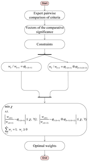
Figure 1.
FUCOM algorithm.
The proposed modification of FUCOM in the grey environment (G-FUCOM) allowed the processing of expert preferences despite doubts and lack of information when assessing the significance of the criteria. In the next section, the algorithm of the G-FUCOM methodology is presented, and is graphically shown in Figure 2.
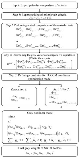
Figure 2.
G-FUCOM methodology.
Step 1. Under the assumption that there are m experts in the observed research and n criteria from the predefined set of evaluation criteria , every expert ranks the criteria by their significance. Ranks of criteria are presented by experts in the descending order (k presents the rank of the observed criterion, ).
Step 2. Perform mutual comparisons of the ranked criteria. The comparison is performed in relation to the first-ranked (the most important) criterion. That way, the importance of the criteria for each expert and for all the criteria ranked in Step 1 are obtained. The importance of the criteria is expressed by experts in grey numbers,. When defining the importance of a criterion, if an expert cannot precisely determine the value of the importance of the criterion, then the expert e defines the upper () and lower limit () of the importance interval. The length of the grey number interval, , expresses the amount of uncertainty that prevails when assessing the importance of the criteria. As the interval increases, the uncertainty in the estimate increases. If there is no uncertainty, then ; i.e., the grey number becomes a white (crisp) number. Thus, for each criterion, we gain the following importance:
Based on the obtained importance of criteria by applying Equation (6), the grey comparative equation (, , where k represents the rank of criteria, ) of the evaluation criteria, is determined:
The obtained vectors of comparative importance of the evaluation criteria are calculated by using Equation (7):
where represents the importance (advantage) of the criterion ranked as compared to the criterion ranked as . The vectors of comparative importance of the evaluation criteria are defined for every expert separately (,,…,,…, , ).
Step 3. Determine the grey vectors of comparative importance (CI) for the experts. Based on the CI vectors of the experts’ answers, , we form vectors of the aggregated sequences of experts, :
where represents grey sequences. For a sequence , we obtain CI vectors ,,…,,…, , for each expert. By applying Equation (9), we obtain the average grey sequence of the CI vectors. We thus obtain the averaged grey CI vector of average responses, :
Step 4. Calculation of the final values of grey weight coefficients of the evaluation criteria . The final values of weight coefficients should meet two conditions:
(1) The relation of weight coefficients should be the same as the CI between the observed criteria (), which is defined in Step 3, and meets the condition:
(2) In addition to the mentioned condition, the final values of weight coefficients should meet the condition that :
The nonlinear model for determining weight coefficients can be defined as follows:
where is the grey weight coefficient of a criterion.
By solving the model in (12), the final values of the evaluation criteria, , and the deviation from full consistency, (DFC) , are obtained.
6. Multicriteria Optimization of Logistics Processes: Grey SWOT-FUCOM Model
The implementation of the grey SWOT-FUCOM model was carried out in two phases. In the first phase, the analysis of the current situation was performed, and the advantages of the future system (barcode system) were investigated by applying the SWOT analysis, which allowed us to gain insight into the advantages/disadvantages of the existing way of organizing the process in the company’s warehousing system, as well as a new way of organizing the process by applying barcode technology. In the second phase, the evaluation and ranking of the SWOT matrix elements were performed using the grey FUCOM model and the grey Hamy operator.
The grey SWOT-FUCOM model was tested in the technical material warehouse and receiving warehouse of the Natron-Hayat Company in Bosnia and Herzegovina. The technical material warehouse is part of Natron-Hayat, and represents an important logistics element for the company. Therefore, the optimization of logistics processes in the warehouse was crucial to accelerating the process of removing goods from the warehouse. One way to optimize the process was to introduce barcode technology into the warehouse.
6.1. SWOT Analysis
A SWOT analysis is an efficient tool for understanding and making decisions in a variety of situations in the work of a company or organization. The following section presents the criteria for the SWOT analysis of the observed technical material warehouse at Natron-Hayat.
Strength refers to an inner quality; i.e., the capabilities of a company. Strengths should be sought in areas in which a particular company stands out from its competitors and in which it succeeds. These can include: quality and competitiveness, reputation, market share, customers, professional and motivated personnel, good organization and management, technical equipment, valuable and useful assets, profitability, liquidity, creditworthiness, and/or geographical location. In this part of the SWOT analysis, the strengths of the company in the receiving warehouse and technical material warehouse were determined, and are shown in Figure 3.
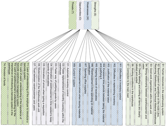
Figure 3.
SWOT factors.
Weaknesses also relate to internal characteristics; i.e., the capabilities of a company. Weaknesses can all be listed according to the strengths, as they refer to a lack of certain strengths, such as a bad image, unprofessional and unmotivated personnel, a lack of necessary assets and money (weak balance sheet), or a lack of creditors. During work, certain weaknesses in a system can be identified that could be eliminated by introducing a barcode system. Weaknesses in the functioning of the warehouses are presented in Figure 3.
Opportunities are immanent in any business. They originate from the environment in which the company operates or intends to operate. However, this analysis included only those opportunities that the company, with its current strengths and weaknesses, can, or could in some circumstances, realize. In order for an opportunity to be realized, the engagement of the company is necessary, along with the necessary strengths. The opportunities provided in the technical material warehouse by introducing barcode technology are presented in Figure 3.
Unlike opportunities, a company’s threats usually cannot be influenced, so a company needs to be prepared for them in time. Threats can be numerous, but they all relate to declining revenues, rising costs, and falling profits, and jeopardize the company’s survival. Threats that can occur when implementing a barcode system are presented in Figure 3.
6.2. FUCOM-G: Evaluation of SWOT Factors
This section presents the application of the FUCOM-G approach to determine the weights of the SWOT factors. Three experts who evaluated the SWOT factors participated in the research. The experts were employed in the company’s warehousing system in managerial positions, and they were familiar with the issues being studied. The evaluation of the SWOT factors was carried out using a nine-point grey scale: equal importance = [1.0,1.5]; pretty low importance = [1.5,2.5]; low importance = [2.5,3.5], slightly low importance = [3.5,4.5], essential importance = [4.5,5.5], slightly strong importance = [5.5,6.5], very strong importance = [6.5,7.5], exceedingly high importance = [7.5,8.5], and absolute importance = [8.5,9.5]. Since we performed a hierarchical division of the SWOT factors into two levels in the SWOT analysis, the FUCOM-G model was applied separately to each of the levels. Thus, for the first level, the S, W, O, and T factors were evaluated; i.e., one FUCOM-G model was formed. For the second level, the FUCOM-G model was applied to each of the groups of S, W, O, and T subfactors. So, for the second level, a total of four FUCOM-G models were defined. The procedure for defining the FUCOM-G model for both levels of the SWOT analysis is explained further elsewhere in this paper.
6.2.1. Level I of the SWOT Matrix: Defining the Weights of the Main Dimensions
Step 1. Ranking criteria. In the first step, the experts performed the ranking of criteria according to the following: E1: ; E2: ; and E3: .
Step 2. Determining the importance of SWOT factors. In the second step, the experts performed a pairwise comparison of the previously ranked factors (Step 1). The comparisons were made in relation to the first-ranked factor, and on the basis of a nine-point grey scale. The importance of the SWOT factors were determined for each expert individually, and are presented below:
Based on the obtained importance of criteria by applying Equation (6), the grey comparative importance, , of the evaluation criteria and vectors of comparative importance, , were determined. Based on the obtained significance of the factors, the comparative significance of the criteria for the first expert was calculated as:
In the same way, the vectors of the comparative importance of the SWOT factors for other experts were obtained as: ; ; ; ; ; and .
Thus, we obtained the vectors of comparative importance of the SWOT factors:
Step 3. Determine the average grey vectors of comparative importance (CI) for the experts. In order to obtain the aggregated interval grey CI vectors of the experts’ answers, , we used a grey-number HM operator. Thus, based on (Step 2) and Equation (4), we obtained an element, , in the aggregated interval grey CI () vector as follows.
Based on the presented values of and assuming that , at the position , the following value is aggregated:
Thus, we obtained the aggregate value In the same way, the aggregation of other elements of the aggregated interval grey CI () vectors was performed:
Step 4. The final grey values of the weighting coefficients must satisfy two conditions:
(1) The final grey values of the weighting coefficients should satisfy condition (10); i.e., that:
(2) In addition to condition (10), the final value of the weighting coefficients should satisfy condition (11):
By applying Equation (12), a model for determining the optimal values of grey weighting coefficients was defined:
By solving this model, we obtained the final values of the grey weighting coefficients: , , , and ; and a deviation from complete consistency .
Based on the obtained values for the weighting coefficients, we concluded that the most important element of the main dimensions of the SWOT analysis was the weaknesses. The reason for this was that the weaknesses were the basic problem in the work at the technical material warehouse, and needed to be improved by introducing barcode technology.
6.2.2. Level II of the SWOT Matrix: Defining the Weights of S, W, O, and T Factors
Step 1. Ranking criteria. The experts performed the ranking of criteria according to the following:
(a) Strength factors: E1: S3>S2>S1=S4>S5=S6>S7; E2: S3>S2=S1>S4>S5>S6>S7; and E3: S3>S2>S1>S4=S5>S6>S7;
(b) Weakness factors: E1: C3=C4>C5>C2=C1>C6=C8>C7>C9, E2: C3>C4>C5>C2=C1>C6>C8=C7=C9 and E3: C3=C4=C5>C2=C1>C6=C8>C7>C9;
(c) Opportunity factors: E1: C4=C3>C2>C1>C5=C7>C6, E2: C4>C3>C2>C1>C5=C7>C6 and E3: C4=C3>C2=C1>C5>C7=C6;
(d) Threat factors: E1: C4>C1>C3>C2, E2: C4>C1>C3>C2 and E3: C4>C1>C3>C2.
Step 2. Determine the importance of S, W, O, and T factors. In the second step, the experts performed a pairwise comparison of previously ranked factors (Step 1). The importance of the S, W, O, and T factors were determined for each expert individually, and are presented below:
Based on the obtained importance of criteria by applying Equation (6), we determined the grey comparative importance, , of the S, W, O, and T factors; and the vectors of comparative importance: , , , and :
Step 3. Determine the average grey vectors of comparative importance (CI) for the experts. For obtaining the aggregated interval grey CI vectors of the experts’ answers—, , , and —we used a grey-number HM operator. Thus, we obtained the aggregate values of the CI vectors:
Step 4. The final grey values of the weighting coefficients , , and should satisfy conditions (10) and (11), which were an integral part of the model (12).
By solving the presented models, the optimal values of the grey weighting coefficients were obtained, and are shown in Table 1.

Table 1.
Optimal values of weighting coefficients of S, W, O, and T factors.
Grey weighting coefficients of both hierarchical levels of the SWOT-FUCOM model, including global and local rank factors, are shown in Table 2 and Figure 4.
Table 2.
Global and local weight values of SWOT factors.
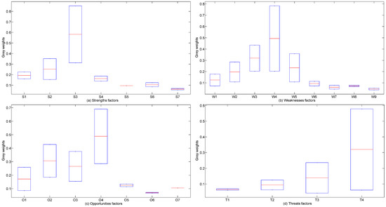
Figure 4.
Local weight values of SWOT factors.
Based on the results shown in Table 2, for the local rank, we concluded that the most important element of the strength (S) dimension was good work organization within the work unit. In the S dimension, seven elements were identified, the third of which was the most important, and implied good work organization within the work unit. This was the result of the company’s investment in human resources to provide support for its employees’ education and training. In addition, the company had a large number of young personnel who were willing and able to work in teams and be further trained. The relationships between warehouse workers and users and the labeling of all items were less-important elements of this dimension. The least important elements were the working conditions in the warehouse and the connection to the main road.
In order to confirm the obtained results, a comparison with the crisp FUCOM methodology was performed. The results in Figure 4 show that there were minor discrepancies between the results of the G-FUCOM and the crisp FUCOM methodologies.
However, such deviations were expected, as the G-FUCOM algorithm handled interval values that contained certainties and uncertainties in the information, while the crisp FUCOM algorithm ignored such information. After comparing the presented results (Figure 5a–d), we concluded that by applying both methodologies, the same priority of factors within the considered cluster was maintained (S, W, O, and T). Based on the presented results, we concluded that the results of the G-FUCOM algorithm were confirmed, and that the defined significance of the factors was credible.
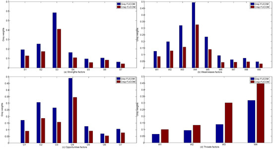
Figure 5.
Comparisons of the results of the G-FUCOM and crisp FUCOM methodologies.
The most important elements of the weakness (W) dimension were: the problem with the method of justifying the material taken, and the excessive time periods between taking the material and justifying it. The final values of W3 and W4 were approximate: W3 = [0.064,0.251] and W4 = [0.064,0.452]. The problem with the method of justifying the material taken occurred due to the diversity of the assortment in the warehouse and the similarities of the names of the items, and, due to that, errors occurred. These mistakes were made by the users who took the material from the warehouse, and subsequently justified it through the system. This was especially visible in cases of a longer period of time between taking the material and justifying it, as it happened that the user did not immediately justify the material. The reason for this was the excessive volume of work in both production and maintenance of the plant, so users offered their justifications subsequent to taking the material.
In addition to strengths and weaknesses, the most important elements of the opportunity (O) dimension were: the elimination of errors when typing requisitions and a faster way of justifying the use of goods by users. The final values for O4 and O3 were: O4 = [0.073,0.202] and O3 = [0.040,0.110]. For the O4 element, the introduction of the barcode system eliminated the occurrence of errors when typing purchase orders, since the warehouse worker immediately provided the purchase order when issuing materials. On the other hand, the barcode system was incomparably faster, as it worked on the principle of automatic reading of the code and automatic creation of the purchase order by the warehouse worker for the material issued.
After the calculation, it was concluded that the most important element of the threat (T) dimension was the provision of funds. The final value for T4 = [0.011,0.153]. In the introduction of this technology, it was necessary to allocate certain financial resources that were needed for the purchase of equipment, education of warehouse workers, printing barcodes, installing additional software, etc.
At the level of global rank, the most important element was the good work organization within the work unit. Within the global rank, the final value for this element was S3 = [0.079,0.227]. Good organization was closely related to the strength of the work unit, and was present at the time. The performance of this organization could be further improved by introducing barcode technology. Realistic indicators of the functioning of the company’s current warehousing system were obtained through research and application of an integrated model that included the FUCOM-G method of multicriteria decision making and a SWOT analysis. When applying the methods of MCDM, it is possible to select adequate strategies, rationalize certain logistics and other processes, and make adequate decisions that have an impact on the performance of companies or their subsystems.
7. Conclusions
The proposed model presented in the paper was an integration of the grey FUCOM and SWOT methods, in which the SWOT analysis was used to identify the S, W, O, and T factors of a logistics company, and grey FUCOM was used to calculate the weight values of the SWOT matrix factors. The model was verified through a case study of the logistics company Natron-Hayat in Bosnia and Herzegovina. The SWOT-FUCOM-G model was implemented through an analysis of the implementation of barcode technology in the Natron-Hayat warehousing system. In order to obtain the most realistic indicators, we formed a SWOT matrix with a total of 27 elements that were evaluated. The conducted research had dual contributions that were reflected in both scientific and practical aspects.
One of the greatest contributions of this paper was enriching the methodology of multicriteria decision making by introducing a new model that involved the integration of a SWOT matrix and the FUCOM method in a grey environment. Additionally, as a special contribution, it was necessary to include a novel grey Hammy aggregator (GHA), which provided objective aggregation of expert decisions. The implementation of the GHA enabled better recognition of inaccuracies and subjectivity that occurred during group decision making. The development of these models contributed to the improvement of the MCDM literature. The proposed models allowed the evaluation of elements despite the inaccuracies and lack of quantitative information in a decision-making process. The third contribution of the paper was the improvement of the methodology for evaluating logistics processes, since the application of this or a similar approach in the field of logistics had not been considered previously.
If the contributions are observed from a practical aspect, we can emphasize that the evaluation of the conditions for the application of barcode technology in this part of the company provided an adequate basis for increasing the efficiency of its logistics operations. Increasing its efficiency also enabled an increase in the efficiency of the entire supply chain, in which a large number of users participate when considering the volume of company’s operations.
After conducting the SWOT analysis presented in this paper, a number of shortcomings that occurred in the current work at the company were pointed out. By introducing barcode technology at the company, the flow of materials to end users increased. This sped up the implementation of customer service.
As the barcode is one of the most common technologies for marking items, it allows unambiguous identification of items and speeds up their flow. In addition, the introduction of barcode technology could lead to a reduction in the level of errors when working in the warehouse. The transition from the old system to the barcode system can be achieved through positive effects, and this was proven through the integrated model in this paper.
The one of limitations of the developed approach was the complex mathematical process for computing criteria weights. The increase in the number of input parameters in the research further complicated the application of this approach. Such a limitation can be eliminated by creating a software solution that is user-oriented and that allows a wider application of the presented approach for solving problems in practice. Through the computation in this study, the authors developed a software solution based on the application of MATLAB and Microsoft Excel software packages.
By using this approach, it is possible to easily evaluate logistics processes that have a significant impact on the efficiency of an entire supply chain. The SWOT-FUCOM-G model, with minor modifications, can also be used to analyze other business processes. It is also applicable in evaluation processes in other areas such as human-resource management [58], marketing [59], and railway lines [60], and it may be particularly suitable for manufacturing companies [61]. The flexibility of the model is reflected in the possibility of integrating other methods of multicriteria decision making that will enable the evaluation of proposed strategies and the selection of the optimum one, which will certainly be considered in future research. In addition, further research related to this paper can refer to the application of other theories of uncertainty in the proposed model.
Author Contributions
Conceptualization, D.P. and Ž.S.; methodology, D.P., Ž.S. and V.L.; validation, S.J., V.P. and D.P.; formal analysis, Ž.S.; investigation, Ž.S.; writing—review and editing, D.P., Ž.S., V.L., S.J. and V.P.; supervision, D.P. and Ž.S. All authors have read and agreed to the published version of the manuscript.
Funding
This research received no external funding.
Institutional Review Board Statement
Not applicable.
Informed Consent Statement
Not applicable.
Data Availability Statement
Not applicable.
Acknowledgments
The authors wish to acknowledge the support received from the College of Applied Technical Sciences Niš.
Conflicts of Interest
The authors declare no conflict of interest.
Appendix A
The symbols used in this paper, their notations, and their respective values are provided in Table A1 for clarity.
Table A1.
Symbols and semantics.
Table A1.
Symbols and semantics.
| Symbol | Meaning |
|---|---|
| Hamy operator | |
| Grey number Hamy operator | |
| Grey number | |
| m | Number of experts |
| Set of criteria | |
| Importance of criterion j on kth rank | |
| Grey comparative importance of criteria on kth rank determined by eth expert | |
| Vector of comparative importance determined by eth expert | |
| Grey weight coefficients of criteria | |
| A deviation from full consistency | |
| Sj | Strength factors |
| Wj | Weaknesses factors |
| Oj | Opportunities factors |
| Tj | Threats factors |
Appendix B
Proof.
Based on the operations with RN:
In addition, since:
then represents GN, so Theorem 1 has been proved. □
References
- Stević, Ž.; Stjepanović, Ž.; Božičković, Z.; Das, D.K.; Stanujkić, D. Assessment of Conditions for Implementing Information Technology in a Warehouse System: A Novel Fuzzy Piprecia Method. Symmetry 2018, 10, 586. [Google Scholar] [CrossRef] [Green Version]
- Pupavac, D. Warehouse Logistics Management. Bus. Logist. Mod. Manag. 2012, 12, 87–98. [Google Scholar]
- Stević, Ž.; Vasiljević, M.; Puška, A.; Tanackov, I.; Junevičius, R.; Vesković, S. Evaluation Of Suppliers under Uncertainty: A Multiphase Approach Based on Fuzzy Ahp and Fuzzy Edas. Transport 2019, 34, 52–66. [Google Scholar] [CrossRef] [Green Version]
- Kosanke, L.; Schultz, M. Key Performance Indicators for Performance-Based Airport Management from the perspective of airport operations. In Proceedings of the CATO, Delft, The Netherlands, 20–23 July 2015. [Google Scholar]
- Rauch, P. SWOT analyses and SWOT strategy formulation for forest owner cooperations in Austria. Eur. J. For. Res. 2007, 126, 413–420. [Google Scholar] [CrossRef]
- Chae, B. Developing key performance indicators for supply chain: An industry perspective. Supply Chain Manag. Int. J. 2009, 14, 422–428. [Google Scholar] [CrossRef]
- Đalić, I.; Stević, Ž.; Ateljević, J.; Turskis, Z.; Zavadskas, E.K.; Mardani, A. A Novel Integrated Mcdm-Swot-Tows Model for The Strategic Decision Analysis In Transportation Company. Facta Univ. Ser. Mech. Eng. 2021, 19, 401–422. [Google Scholar] [CrossRef]
- Kurttila, M.; Pesonen, M.; Kangas, J.; Kajanus, M. Utilizing the analytic hierarchy process AHP in SWOT analysis—A hybrid method and its application to a forest-certification case. For. Policy Econ. 2000, 1, 41–52. [Google Scholar] [CrossRef]
- Chang, H.-H.; Huang, W.-C. Application of a quantification SWOT analytical method. Math. Comput. Model. 2006, 43, 158–169. [Google Scholar] [CrossRef]
- Ananda, J.; Herath, G. The use of Analytic Hierarchy Process to incorporate stakeholder preferences into regional forest planning. For. Policy Econ. 2003, 5, 13–26. [Google Scholar] [CrossRef]
- Moslem, S.; Farooq, D.; Ghorbanzadeh, O.; Blaschke, T. Application of the AHP-BWM Model for Evaluating Driver Behavior Factors Related to Road Safety: A Case Study for Budapest. Symmetry 2020, 12, 243. [Google Scholar] [CrossRef] [Green Version]
- Moslem, S.; Çelikbilek, Y. An integrated grey AHP-MOORA model for ameliorating public transport service quality. Eur. Transp. Res. Rev. 2020, 12, 68. [Google Scholar] [CrossRef]
- Duleba, S.; Çelikbilek, Y.; Moslem, S.; Esztergár-Kiss, D. Application of grey analytic hierarchy process to estimate mode choice alternatives: A case study from Budapest. Transp. Res. Interdiscip. Perspect. 2022, 13, 100560. [Google Scholar] [CrossRef]
- Gündoğdu, F.K.; Duleba, S.; Moslem, S.; Aydın, S. Evaluating public transport service quality using picture fuzzy analytic hierarchy process and linear assignment model. Appl. Soft Comput. 2021, 100, 106920. [Google Scholar] [CrossRef]
- Ho, W. Integrated analytic hierarchy process and its applications–A literature review. Eur. J. Oper. Res. 2008, 186, 211–228. [Google Scholar] [CrossRef]
- Leskinen, L.A.; Leskinen, P.; Kurttila, M.; Kangas, J.; Kajanus, M. Adapting modern strategic decision support tools in the participatory strategy process—A case study of a forest research station. For. Policy Econ. 2006, 8, 267–278. [Google Scholar] [CrossRef]
- Taleai, M.; Mansourian, A.; Sharifi, A. Surveying general prospects and challenges of GIS implementation in developing countries: A SWOT–AHP approach. J. Geogr. Syst. 2009, 11, 291–310. [Google Scholar] [CrossRef]
- Masozera, M.K.; Alavalapati, J.R.R.; Jacobson, S.K.; Shresta, R.K. Assessing the suitability of community-based management for the Nyungwe Forest Reserve, Rwanda. For. Policy Econ. 2006, 8, 206–216. [Google Scholar] [CrossRef]
- Stewart, R.A.; Mohamed, S.; Daet, R. Strategic implementation of IT/IS projects in construction: A case study. Autom. Constr. 2002, 11, 681–694. [Google Scholar] [CrossRef] [Green Version]
- Shresthaa, R.K.; Alavalapati, R.R.; Kalmbacher, R.S. Exploring the potential for silvopasture adoption in South-Central Florida: An application of SWOT–AHP method. Agric. Syst. 2004, 81, 185–199. [Google Scholar] [CrossRef]
- Pamučar, D.; Ćirović, G.; Sekulović, D. Development of an integrated transport system in distribution centres: A FA’WOT analysis. Teh. Vjesn. 2015, 22, 649–658. [Google Scholar] [CrossRef] [Green Version]
- Al Mustafa, S.A.; Khan, M.; Hussain, M. Implementing Barcode Medication Administration Systems in Public Sector Medical Units. Int. J. Decis. Support Syst. Technol. 2018, 10, 23–39. [Google Scholar] [CrossRef] [Green Version]
- Alharthi, H.; Sultana, N.; Al-Amoudi, A.; Basudan, A. An Analytic Hierarchy Process-based Method to Rank the Critical Success Factors of Implementing a Pharmacy Barcode System. Perspect. Health Inf. Manag. 2015, 12, 1g. [Google Scholar]
- Nathnail, E.; Gogas, M.; Adamos, G. Urban Freight Terminals: A Sustainability Cross-case Analysis. Transp. Res. Procedia 2016, 16, 394–402. [Google Scholar] [CrossRef] [Green Version]
- Stoilova, S.; Kunchev, L. Study of criteria for evaluation of transportation with intermodal transport. In Proceedings of the 16th International Scientific Conference Engineering for Rural Development, Jelgava, Latvia, 24–26 May 2017; pp. 349–357. [Google Scholar]
- Carlucci, D. Evaluating and selecting key performance indicators: An ANP-based model. Meas. Bus. Excel. 2010, 14, 66–76. [Google Scholar] [CrossRef]
- Alvandi, M.; Fazli, S.; Yazdani, L.; Aghaee, M. An Integrated MCDM Method in Ranking BSC Perspectives and key Performance Indicators (KPIs). Manag. Sci. Lett. 2012, 2, 995–1004. [Google Scholar] [CrossRef]
- Mladenovic, G.; Vajdic, N.; Wündsch, B.; Salaj, A.T. Use of key performance indicators for PPP transport projects to meet stakeholders’ performance objectives. Built Environ. Proj. Asset Manag. 2013, 3, 228–249. [Google Scholar] [CrossRef]
- Podgórski, D. Measuring operational performance of OSH management system–A demonstration of AHP-based selection of leading key performance indicators. Saf. Sci. 2015, 73, 146–166. [Google Scholar] [CrossRef] [Green Version]
- Sénquiz-Díaz, C. The Effect of Transport and Logistics on Trade Facilitation and Trade: A PLS-SEM Approach. Economics 2021, 9, 11–24. [Google Scholar] [CrossRef]
- Durmić, E.; Stević, Ž.; Chatterjee, P.; Vasiljević, M.; Tomašević, M. Sustainable supplier selection using combined FUCOM–Rough SAW model. Rep. Mech. Eng. 2020, 1, 34–43. [Google Scholar] [CrossRef]
- Solakivi, T.; Ojala, L.; Laari, S.; Lorentz, H.; Toyli, J.; Malmsten, J.; Viherlehto, N. Finland State of Logistics 2014; University of Turku: Turku, Finland, 2015. [Google Scholar]
- Roy, J.; Chatterjee, K.; Bandhopadhyay, A.; Kar, S. Evaluation and selection of Medical Tourism sites: A rough AHP based MABAC approach. arXiv 2016, arXiv:1606.08962. [Google Scholar]
- Chattopadhyay, R.; Das, P.P.; Chakraborty, S. Development of a Rough-MABAC-DoE-based Metamodel for Supplier Selection in an Iron and Steel Industry. Oper. Res. Eng. Sci. Theory Appl. 2022. [Google Scholar] [CrossRef]
- Jeon, C.M.; Amekudzi, A.A.; Guensler, R.L. Evaluating Plan Alternatives for Transportation System Sustainability: Atlanta Metropolitan Region. Int. J. Sustain. Transp. 2010, 4, 227–247. [Google Scholar] [CrossRef]
- Cadena, P.C.B.; Magro, J.M.V. Setting the Weights of Sustainability Criteria for the Appraisal of Transport Projects. Transport 2015, 30, 298–306. [Google Scholar] [CrossRef] [Green Version]
- Sremac, S.; Stević, Ž.; Pamučar, D.; Arsić, M.; Matić, B. Evaluation of a Third-Party Logistics (3PL) Provider Using a Rough SWARA–WASPAS Model Based on a New Rough Dombi Agregator. Symmetry 2018, 10, 305. [Google Scholar] [CrossRef] [Green Version]
- Badi, I.; Abdulshahed, A.M.; Shetwan, A.G. A Case Study of Supplier Selection for A Steelmaking Company in Libya by Using the Combinative Distance-Based Assessment (CODAS) Model. Decis. Mak. Appl. Manag. Eng. 2018, 1, 16–33. [Google Scholar] [CrossRef]
- Stević, Ž.; Pamučar, D.; Zavadskas, E.K.; Ćirović, G.; Prentkovskis, O. The Selection of Wagons for the Internal Transport of a Logistics Company: A Novel Approach Based on Rough BWM and Rough SAW Methods. Symmetry 2017, 9, 264. [Google Scholar] [CrossRef] [Green Version]
- Radović, D.; Stević, Ž.; Pamučar, D.; Zavadskas, E.K.; Badi, I.; Antuchevičiene, J.; Turskis, Z. Measuring Performance in Transportation Companies in Developing Countries: A Novel Rough ARAS Model. Symmetry 2018, 10, 434. [Google Scholar] [CrossRef] [Green Version]
- Pamučar, D.; Sremac, S.; Stević, Ž.; Ćirović, G.; Tomić, D. New multi-criteria LNN WASPAS model for evaluating the work of advisors in the transport of hazardous goods. Neural Comput. Appl. 2019, 31, 5045–5068. [Google Scholar] [CrossRef]
- Pamučar, D.; Vasin, L.; Atanasković, P.; Miličić, M. Planning the City Logistics Terminal Location by Applying the Greenp-Median Model and Type-2 Neurofuzzy Network. Comput. Intell. Neurosci. 2016, 2016, 6972818. [Google Scholar] [CrossRef] [Green Version]
- Akyuz, G.A.; Erkan, T.E. Supply chain performance measurement: A literature review. Int. J. Prod. Res. 2009, 48, 5137–5155. [Google Scholar] [CrossRef]
- Wong, C.Y.; Karia, N. Explaining the competitive advantage of logistics service providers: A resource-based view approach. Int. J. Prod. Econ. 2010, 128, 51–67. [Google Scholar] [CrossRef]
- Qureshi, M.; Kumar, D.; Kumar, P. An integrated model to identify and classify the key criteria and their role in the assessment of 3PL services providers. Asia Pac. J. Mark. Logist. 2008, 20, 227–249. [Google Scholar] [CrossRef]
- Shaik, M.; Abdul-Kader, W. Performance measurement of reverse logistics enterprise: A comprehensive and integrated approach. Meas. Bus. Excel. 2012, 16, 23–34. [Google Scholar] [CrossRef]
- Deng, J.L. Grey Control Systems; Press of Huazhong University of Science and Technology: Wuhan, China, 1985. [Google Scholar]
- Deng, J.L. Introduction to grey system theory. J. Grey Syst. 1989, 1, 1–24. [Google Scholar]
- Liu, S.F. On Perron-Frobenius theorem of grey nonnegative matrix. J. Grey Syst. 1989, 1, 157–166. [Google Scholar]
- Mardani, A.; Nilashi, M.; Zavadskas, E.K.; Awang, S.R.; Zare, H.; Jamal, N.M. Decision Making Methods Based on Fuzzy Aggregation Operators: Three Decades Review from 1986 to 2017. Int. J. Inf. Technol. Decis. Mak. 2018, 17, 391–466. [Google Scholar] [CrossRef]
- Zadeh, L.A. Fuzzy sets. Inf. Control. 1965, 8, 338–353. [Google Scholar] [CrossRef] [Green Version]
- Ali, Y.; Ahmad, M.; Sabir, M.; Shah, S.A. Regional development through energy infrastructure: A comparison and optimization of Iran-Pakistan-India (IPI) & Turkmenistan-Afghanistan-Pakistan-India (TAPI) gas pipelines. Oper. Res. Eng. Sci. Theory Appl. 2021, 4, 82–106. [Google Scholar] [CrossRef]
- Gorcun, O.F.; Senthil, S.; Küçükönder, H. Evaluation of tanker vehicle selection using a novel hybrid fuzzy MCDM technique. Decis. Mak. Appl. Manag. Eng. 2021, 4, 140–162. [Google Scholar] [CrossRef]
- Sharma, H.K.; Kumari, K.; Kar, S. Forecasting Sugarcane Yield of India based on rough set combination approach. Decis. Mak. Appl. Manag. Eng. 2021, 4, 163–177. [Google Scholar] [CrossRef]
- Sharma, H.K.; Singh, A.; Yadav, D.; Kar, S. Criteria selection and decision making of hotels using Dominance Based Rough Set Theory. Oper. Res. Eng. Sci. Theory Appl. 2022. [Google Scholar] [CrossRef]
- Hara, T.; Uchiyama, M.; Takahasi, S.E. A refinement of various mean inequalities. J. Inequal. Appl. 1998, 2, 387–395. [Google Scholar] [CrossRef]
- Pamučar, D.; Stević, Ž.; Sremac, S. A New Model for Determining Weight Coefficients of Criteria in MCDM Models: Full Consistency Method (FUCOM). Symmetry 2018, 10, 393. [Google Scholar] [CrossRef] [Green Version]
- Dâmbean, C.A.; Gabor, M.R. Implications of Emotional Intelligence in Human Resource Management. Econ. Innov. Econ. Res. 2021, 9, 73–90. [Google Scholar] [CrossRef]
- Karamaşa, Ç.; Ergün, M.; Gülcan, B.; Korucuk, S.; Memiş, S.; Vojinović, D. Rankıng value-creatıng green approach practıces ın logıstıcs companıes operatıng ın the TR A1 regıon and choosıng ıdeal green marketıng strategy. Oper. Res. Eng. Sci. Theory Appl. 2021, 4, 21–38. [Google Scholar] [CrossRef]
- Fosu, P. Does Railway Lines Investments Matter for Economic Growth? Econ. Innov. Econ. Res. 2021, 9, 11–24. [Google Scholar] [CrossRef]
- Messinis, S.; Vosniakos, G. An agent-based Flexible Manufacturing System controller with Petri-net enabled algebraic deadlock avoidance. Rep. Mech. Eng. 2020, 1, 77–92. [Google Scholar] [CrossRef]
Publisher’s Note: MDPI stays neutral with regard to jurisdictional claims in published maps and institutional affiliations. |
© 2022 by the authors. Licensee MDPI, Basel, Switzerland. This article is an open access article distributed under the terms and conditions of the Creative Commons Attribution (CC BY) license (https://creativecommons.org/licenses/by/4.0/).