The Regulation of an Electric Oven and an Inverted Pendulum

Abstract

In this research, a proportional integral derivative regulator, a first-order sliding-mode regulator, and a second-order sliding-mode regulator are compared, for the regulation of two different types of mathematical model. A first-order sliding-mode regulator is a method where a sign-mapping checks that the error decays to zero after a convergence time; it has the problem of chattering in the output. A second-order sliding-mode regulator is a smooth method to counteract the chattering effect where the integral of the sign-mapping is used. A second-order sliding-mode regulator is presented as a new class of algorithm where the trajectory is asymptotic and stable; it is shown to greatly improve the convergence time in comparison with other regulators considered. Simulation and experimental results are described in which an electric oven is considered as a stable linear mathematical model, and an inverted pendulum is considered as an asymmetrical unstable non-linear mathematical model.

1. Introduction

There are several kinds of controls: proportional integral derivative (PID) controls are studied in [1,2], model-based controls are discussed in [3,4], and disturbance rejection controls are designed in [5,6]. For these controls, there are two types of objective—tracking, which involves the following of a time-varying set point, and regulation, which involves the following of a constant set point. This research focuses on regulation. Three types of regulators are studied to achieve regulation—one is a proportional integral derivative (PID) regulator, and the other two are types of sliding-mode regulator.

The PID regulator is frequently considered in the literature—any proposed regulator must have better characteristics than the PID regulator. Therefore, here, a PID regulator is compared with a sliding-mode regulator, with the purpose of determining if there is a regulator that can replace the PID regulator.

The sliding-mode regulator is a method that contributes greatly to enabling a mathematical model to follow a set point. The method can work with linear or non-linear mathematical models, and is a robust regulator that can be applied to asymmetrical mathematical models, such as different types of inverted pendulums. A further advantage of a sliding-mode regulator is that it provides good results when there are coupled disturbances in a mathematical model.

In this research, two sliding-model regulators are used for the regulation of two mathematical models; one is a first-order sliding-mode regulator, and the other is a second-order sliding-mode regulator. A first-order sliding-mode regulator is a method where a sign-mapping checks that the error decays to zero after a convergence time. One problem associated with a first-order sliding-mode regulator is chattering in the output. One of the ways to reduce this chattering is by increasing the order of the regulator; a second-order sliding-mode regulator is a smooth method to counteract the chattering effect where the integral of the sign-mapping is used [7,8,9]. It is possible to achieve optimal responses in a second-order sliding-mode regulator with respect to the input noises by means of exact differentiators.

Some authors who have worked with second-order sliding-mode regulators are [10,11,12], who have sought to increase the order of sign-mapping in the regulator to attenuate the chattering that occurs. In [13,14], a robust regulator applied to a delta robot was designed, where the regulator did not require exact knowledge of the mathematical model and used an approximate estimation, guaranteeing a reduction in errors.

Most authors have used the Lyapunov method to assess the gains associated with the use of first-ordersliding-mode regulators [7,8,9], and of second-ordersliding-mode regulators [10,11,12]. In contrast to the previous research, this paper uses the pole assignment method of [15,16,17], as analternative approach to determining gains associated with the use of first- and second-order sliding-mode regulators

Simulation and experimental results are described for an electric oven, considered as an example of a stable linear mathematical model, and for an inverted pendulum, considered as an example of an asymmetric unstable non-linear mathematical model. The electric oven could be used for baking, while the inverted pendulum could be used for the testing of regulators.

2. Mathematical Models of the Electric Oven and Inverted Pendulum

In this section, an electric oven is considered as an example of a stable linear mathematical model, and an inverted pendulum is considered as an example of an asymmetric unstable non-linear mathematical model.

2.1. Mathematical Model of an Electric Oven

For the simplified case of steady heat flow in one direction, the heat transmitted is proportional to the area perpendicular to the heat flow, to the conductivity of the material, and to the temperature difference, and is inversely proportional to the thickness [18]:

$$Q=\frac{kA}{x}\left(T_1-T_2\right)$$

(1)

where $Q$ is the heat per unit of time, $k$ is the thermal conductivity, $A$ is the area, $\left(T_1-T_2\right)$ is the temperature difference between the hot and cold parts, and $x$ is the thickness of the material. Considering that $R=\frac{kA}{x}$ where $R$ is the thermal resistivity of the material.

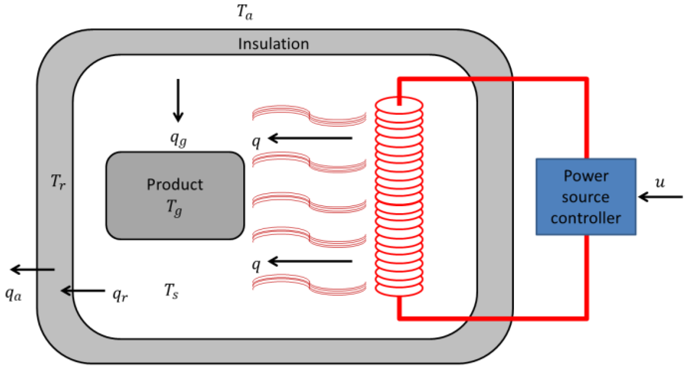
In order to obtain the mathematical model, a free body diagram was designed to exemplify, in a very general way, the composition of the electric oven. This diagram is presented in Figure 1. The Fourier equations that describe the behavior of the electric oven are as follows:

$$\begin{array}{l}\begin{array}{c}{q}_g=R_g\left(T_s-T_g\right)\\ q_r=R_r\left(T_s-T_r\right)\\ \begin{array}{c}{q}_a=R_a\left(T_r-T_a\right)\\ q=ku\end{array}\end{array}\end{array}$$

(2)

where $q$ is the thermal power, $R$ is the coefficient of thermal resistivity, $T$ is the temperature, the subscript $g$ is the product to be heated (aluminum), the subscript $s$ refers to the oven, the subscript $r$ is the insulation, and the subscript $a$ is the air of the environment.

From Figure 1, the heat storage capacity in an electric oven is represented as thermal capacitance. For this mathematical model there are three types of thermal capacitance: the thermal capacitance of the oven, the thermal capacitance of the product to be heated, and the thermal capacitance of the insulation. The equations that represent the thermal capacitances are:

$$\begin{array}{l}\begin{array}{c}{C}_s\frac{d}{dt}{T}_s=q-q_g-q_r\\ C_g\frac{d}{dt}{T}_g=q_g\\ C_r\frac{d}{dt}{T}_r=q_r-q_a\end{array}\end{array}$$

(3)

Considering Equations (1) and (2), the differential equations that describe the mathematical model of the electric oven are as follows:

$$\begin{array}{l}\begin{array}{c}\frac{d}{dt}{T}_s=\frac{R_g\left(T_g-T_s\right)+R_r\left(T_r-T_s\right)+ku}{C_s}\\ \frac{d}{dt}{T}_g=\frac{R_g\left(T_s-T_g\right)}{C_g}\\ \frac{d}{dt}{T}_r=\frac{R_r\left(T_s-T_r\right)+R_a\left(T_a-T_r\right)}{C_r}\end{array}\end{array}$$

(4)

where $q$ is the thermal power, $R$ is the coefficient of thermal resistivity, $T$ is the temperature, the subscript $g$ is the product to be heated (aluminum), the subscript $s$ is the oven, the subscript $r$ is the insulation, the subscript $a$ is the air of the environment,$u$ is the supply of electric potential, $k$ is the thermal conductivity, and $C$ is the thermal capacitance. The values of the constants can be seen in

Table 1. Typical values for an electric oven.

Type	Symbol	Value
Thermal resistance of the product (aluminum)	$R_g$	$37.8$ (W/K·m)
Thermal resistance of oven insulation	$R_r$	$8.64$ (W/K·m)
Thermal resistance of air	$R_a$	$0.24$ (W/K·m)
Thermal capacitance of the product	$C_g$	$4.4$ (kJ/K)
Oven thermal capacitance	$C_s$	$8.8$ (kJ/K)
Thermal capacitance of insulation	$C_r$	$10.164$ (kJ/K)

.

2.2. Mathematical Model of an Inverted Pendulum

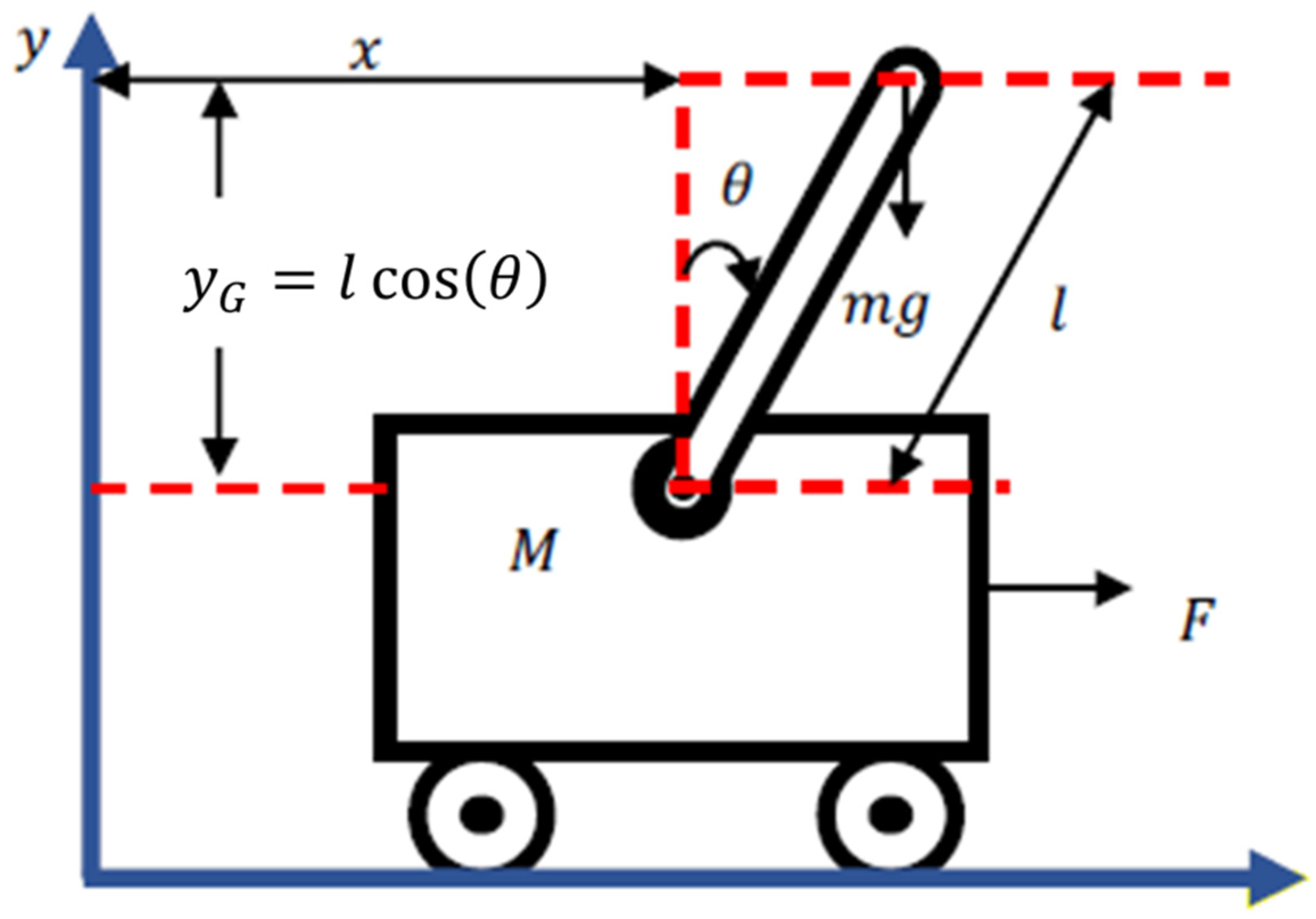
In this section, a mathematical model of the inverted pendulum will be developed; it is represented in Figure 2. For the model, $M$ is the mass of the car, $m$ is the mass of the bar, $x$ is the displacement of the vehicle, $g$ is the gravity, $l$ is the length of the pendulum bar, $\theta$ is the angle that the pendulum bar forms with the axis, and, finally, $F$ is the force applied by the vehicle, which is the regulation variable.

Table 2. Typical values of the inverted pendulum.

Type	Symbol	Value
mass of the car	$M$	$0.5$ (kg)
mass of the bar	$m$	$0.1$ (kg)
length of the pendulum bar	$l$	$0.5$ (m)
gravity	$g$	$9.8$ (m/s2)
moment of inertia	$I$	$0.025$ (kg·m2)

details the inverted pendulum values.

The mathematical model of the inverted pendulum is derived from the Euler–Lagrange equations [19,20,21,22,23]. More details of the mathematical model can be found in [19,20,23,24].

The kinetic energy of the cart is $K_1=\frac{M{\dot{x}}^2}{2}$, the kinetic energy of the pendulum is $K_2=\frac{m{\dot{x}}_G^2}{2}+\frac{m{\dot{y}}_G^2}{2}+\frac{I{\dot{\theta }}_G^2}{2}$, where $x_G=x+l\sin \left(\theta \right),y_G=l\cos \left(\theta \right)$. The kinetic energy is $K=K_1+K_2=\frac{1}{2}\left(M+m\right){\dot{x}}^2+ml\dot{x}\dot{\theta }\cos \left(\theta \right)+\frac{1}{2}\left(I+m{l}^2\right){\dot{\theta }}^2$, and the potential energy is $P=mgl\left(\cos \left(\theta \right)-1\right).$ Substituting $K$ and $P$ into the Lagrangian equation,$L=K-P$ gives:

$$L=\frac{1}{2}\left(M+m\right){\dot{x}}^2+ml\dot{x}\dot{\theta }\cos \left(\theta \right)+\frac{1}{2}\left(I+m{l}^2\right){\dot{\theta }}^2-mgl\left(\cos \left(\theta \right)-1\right)$$

(5)

The equations of the mathematical model can be obtained using the Lagrange equation:

$$\tau =\frac{d}{dt}\left(\frac{\partial L}{\partial \dot{q}}\left(q,\dot{q}\right)\right)-\frac{\partial L}{\partial q}\left(q,\dot{q}\right)$$

(6)

where $q={\left(q_1,\dots ,q_2\right)}^T$ represents the generalized variables, one for each degree of freedom of the mathematical model, and $\tau ={\left({\tau }_1,\dots ,{\tau }_n\right)}^T$ is the force applied to the mathematical model, which is the regulation variable.

In this case, the generalized variables are $x$ and $\theta$; therefore, $q={\left(x,\theta \right)}^T$, and we obtain the elements of each Lagrange equation as follows:

$$\begin{array}{cc}\hfill & \left(\frac{\partial L}{\partial \dot{x}}\right)=\left(M+m\right)\dot{x}+ml\dot{\theta }\cos \left(\theta \right),\hfill \\ \hfill & \left(\frac{\partial L}{\partial x}\right)=0,\hfill \\ \hfill & \left(\frac{\partial L}{\partial \dot{\theta }}\right)=ml\dot{x}\cos \left(\theta \right)+\left(I+m{l}^2\right)\dot{\theta },\hfill \\ \hfill & \left(\frac{\partial L}{\partial \theta }\right)=mgl\sin \left(\theta \right)-ml\dot{x}\dot{\theta }\sin \left(\theta \right),\hfill \\ \hfill \frac{d}{dt}& \left(\frac{\partial L}{\partial \dot{x}}\right)=\left(M+m\right)\ddot{x}+ml\cos \left(\theta \right)\ddot{\theta }-ml\sin \left(\theta \right){\dot{\theta }}^2,\hfill \\ \hfill \frac{d}{dt}& \left(\frac{\partial L}{\partial \dot{\theta }}\right)=ml\cos \left(\theta \right)\ddot{x}+\left(I+m{l}^2\right)\ddot{\theta },\hfill \end{array}$$

(7)

Substituting (7) into (6), the mathematical model of the inverted pendulum can be expressed as seen in Equation (8). The details are shown in [22].

$$\begin{array}{l}\left(M+m\right)\ddot{x}+ml\cos \left(\theta \right)\ddot{\theta }-ml\sin \left(\theta \right){\dot{\theta }}^2=F\\ ml\cos \left(\theta \right)\ddot{x}+\left(I+m{l}^2\right)\ddot{\theta }+ml\sin \left(\theta \right)\dot{x}\dot{\theta }-mgl\sin \left(\theta \right)=0\end{array}$$

(8)

where $x$ is the displacement of the vehicle and $\theta$ is the angular displacement of the pendulum bar with respect to the vehicle, $\dot{x}$ is the linear velocity and $\dot{\theta }$ is the angular velocity. $F$ is the force that is applied to the vehicle to generate a linear displacement. The values of the constants can be seen in the Table 2.

3. Design of a PID Regulator and Two Sliding-Mode Regulators for an Electric Oven

This section presents the three types of regulator for the electric oven; applying a stable linear mathematical model, it is straightforward to determine the regulator gains. The sliding-mode regulators seek to ensure that the error decays to zero after a convergence time [7,8,9]. The regulators considered are robust—when applied to the electric oven of Equation (4) they become insensitive to coupled disturbances.

3.1. PID Regulator Design for an Electric Oven

For the development of the PID regulator, Equation (4) is considered, which describes the behavior of the internal heat of the electric oven. Then Equation (9) is defined as the PID regulator [1,2], where $e=r-y$ is the error, $r$ is the set point, and $y$ is the output.

$$G_c=k_{p}e+T_i{\int }_0^{\infty }edt+T_d\frac{d}{dt}e$$

(9)

Both Equations (4) and (9) obtain their transfer functions, which are then used to determine the PID regulator gains. Equation (4) is expressed in frequency, as follows:

$$G_p=\frac{\left(392s^2+2310s+1750\right)1.6}{\left(3136s^3+37,492s^2+44,750.0s+425\right)}$$

(10)

Equation (9) is expressed in frequency as follows:

$$G_c=\left(k_p+\frac{1}{T_{i}s}+T_{d}s\right)$$

(11)

where $G_p$ corresponds to the behavior of the oven expressed in frequency, and $G_c$ corresponds to the regulator. Equation (11) can be redefined as follows:

$$G_c=\frac{k\left(s+\alpha \right)\left(s+\beta \right)}{s}$$

(12)

To find the regulator gains, we obtain the transfer function that involves Equations (10) and (12). Then, by means of a Hurwitz polynomial, the PID regulator gains are derived, defining the gain $G_c$ which is expressed in the following form:

$$G_c=59.248+\frac{129.67}{s}+5s$$

(13)

From Equation (13), it can be seen that the PID regulator gains are $k_p=59.248$, $k_i=129.67$, and $k_d=5$.

3.2. Design of a First-Ordersliding-Mode Regulator for an Electric Oven

In this section, a first-order sliding-mode regulator applied to the electric oven of Equation (4) is developed.

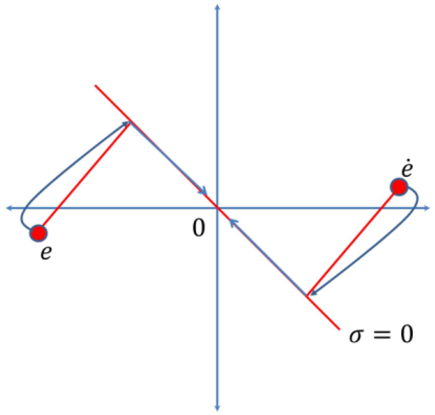
The first-order sliding-mode regulator is invariant and can be written as $\underset{t\to \infty }{\lim }{x}_1,x_2=0\mathrm{if}\mathrm{and}\mathrm{only}\mathrm{if}f\left(x_1,x_2,t\right)=0\sqrt{b^2-4ac}$, where $\left(x_1=\dot{e},x_2=ce\right)$ belong to the distance between the hyperplane and the point. $\left(x_1,x_2\right)$ are known as the error and the derivative of the error. In Figure 3, the behavior of the phase diagram is described, where the states $\left(e,\dot{e}\right)$ tend to slide on the hyperplane $\sigma$, and sigma can be rewritten as in the following equation $\sigma =\dot{e}+ce=0$; the error is $e=r-y,$ where $r$ is the set point and $y$ is the output. The output must reach the set point.

On the other hand, the first-order sliding-mode regulator can be defined in the Equation (14) or (15) [7,8,9]:

$$u=\rho \mathrm{sign}\left(\sigma \right)$$

(14)

$$u=\rho \mathrm{sign}\left(\dot{e}+ce\right)$$

(15)

where the gains $\rho$ and $c>0$ for the mathematical model of the electric oven of the equation (4) are selected by the transfer function of the first-order sliding-mode regulator (15); the sign-mapping $\mathrm{sign}\left(g\left(t\right)\right)$ is changed by one-unit step-mapping $h\left(t\right)$ as follows $\mathrm{sign}\left(g\left(t\right)\right)=2h\left(t\right)-1$.

The transfer function of the first-order sliding-mode regulator (15) is seen in the Equation (16).

$$G_{cctrlMDHor}=2\rho \left(\frac{s+c}{s+1}\right)$$

(16)

Using Equations (10) and (16), and using the feedback model, the transfer function is found as (17).

$$G_{CMDHorP}=\frac{N\left(s\right)}{D\left(s\right)}$$

(17)

where $N\left(s\right)=6272\rho s^3+\left(36,960\rho +6272c\rho \right)s^2+\left(28,000\rho +36,960c\rho \right)s+28,000c\rho$ and $D\left(s\right)=15,680s^4+\left(6272\rho +2.0314\times {10}^5\right)s^3+\left(36,960\rho +6272c\rho +4.1121\times {10}^5\right)s^2+\left(28,000\rho +36,960c\rho +2.2588\times {10}^5\right)s+\left(28,000c\rho +2125\right)$. Equaling to $D\left(s\right)$ with a Hurwitz polynomial, the gains are found as $c=150$ and $\rho =900$.

Figure 3. Phase diagram $\left(e, \dot{e}\right)$.

Figure 3. Phase diagram $\left(e, \dot{e}\right)$.

where the sign function is defined in Equation (16).

$$\begin{array}{ll}\mathrm{sign}(t)=\hfill & \{\begin{array}{l}1\mathrm{if}t>0\hfill \\ -1\mathrm{if}t<0\hfill \end{array}\hfill \end{array}$$

(18)

where the mapping $sign\left(0\right)\in \left[1,-1\right]$ can take a value from 1 to −1.

3.3. Design of a Second-Ordersliding-Mode Regulator for an Electric Oven

One of the problems of the first-order sliding-mode regulator is chattering in the output. One of the ways to reduce this chattering is to increase the order of the regulator, where the integral of $\sigma$ is used. The second-order sliding-mode regulator is defined in Equation (19) [10,11,12].

$$u=c{\left|\sigma \right|}^{\frac{1}{2}}\mathrm{sign}\left(\sigma \right)+m$$

(19)

where $m^{\prime }=b\mathrm{sign}\left(\sigma \right)$ and the hyperplane is ${\sigma }^{\prime }=c{\left|\sigma \right|}^{\frac{1}{2}}\mathrm{sign}\left(\sigma \right)$, sigma can be rewritten as seen in the following equation $\sigma =\dot{e}+ce=0$, the error is $e=r-y,$ where $r$ is the set point, and $y$ is the output. The second-order sliding-mode regulator is composed of both $\sigma$ and ${\sigma }^{\prime },$ with the purpose of reaching $\sigma \to 0$ at finite convergence time. The second-order sliding-mode regulator of Equation (19) can be rewritten as in Equation (20).

$$u=c{\left|\sigma \right|}^{\frac{1}{2}}\mathrm{sign}\left(\sigma \right)+\int \left(b\mathrm{sign}\left(\sigma \right)\right)dt$$

(20)

where the high-frequency sign function is within the integral; the regulator gains $c$ and $b$ for the mathematical model of the electric oven are derived from Equation (4). The gains are selected by the transfer function of the second-order sliding-mode regulator (19), and the sign-mapping $\mathrm{sign}\left(g\left(t\right)\right)$ is changed by one-unit step-mapping $h\left(t\right)$ as follows $\mathrm{sign}\left(g\left(t\right)\right)=2h\left(t\right)-1$.

The transfer function of the second-order sliding-mode regulator (19) is represented in Equation (21).

$$G_{cctrlMD2Hor}=2\left(\frac{c{s}^3+\left(b+2c^2\right)s^2+\left(c^{3}bc\right)s}{s+1}\right)$$

(21)

Using Equations (10) and (21), and the feedback model, the transfer function is found as (22).

$$G_{CMD2HorP}=\frac{N\left(s\right)}{D\left(s\right)}$$

(22)

where $N\left(s\right)=6272c{s}^5+\left(12544c^2+36,960c+6272b\right)s^4+\left(6272b{c}^4+73,920c^2+28,000c+36,960b\right)s^3+\left(36,960b{c}^4+56,000c^2+28,000b\right)s^2+\left(28,000b{c}^4\right)s$ and $D\left(s\right)=6272c{s}^5+\left(12,544c^2+36,960c+6272b+15,680\right)s^4+\left(6272b{c}^4+73,920c^2+28,000c+36,960b+2.0314\times {10}^5\right)s^3+\left(36,960b{c}^4+56,000c^2+28,000b+4.1121\times {10}^5\right)s^2+\left(28,000b{c}^4+2.2588\times {10}^5\right)s+2125$. Equaling to $D\left(s\right),$ with a Hurwitz polynomial, the gains are found as $c=450$ and $b=9000$.

4. Design of a PID Regulator and Two Sliding-Mode Regulators for an Inverted Pendulum

This section presents three types of regulator for the inverted pendulum; as an asymmetrical unstable non-linear mathematical model, it is difficult to determine the regulator gains. The PID regulator and the two sliding-mode regulators are applied in the inverted pendulum of Equation (8) to verify that the regulators considered can be applied to asymmetrical unstable non-linear mathematical models with coupled disturbances.

4.1. PID Regulator Design for an Inverted Pendulum

In this subsection, a PID regulator for an inverted pendulum is designed. The mathematical model is asymmetrical, unstable and non-linear, which complicates the determination of regulator gains. It is necessary to linearize the mathematical model of the inverted pendulum at a desired equilibrium point to find these regulator gains, where the angle $\theta$ and the angular velocity $\dot{\theta }$ are assumed to have small values.

The linearization method is known as an approximate linearization, which is based on a Taylor series expansion to represent an asymmetrical non-linear mathematical model as a linear mathematical model. This method is also known as Jacobian linearization because of the Jacobian matrices that are used for the linear approximation [19,20,23].

For the development of this subsection, the following equation is defined:

$$\begin{array}{c}{x^{\prime }}_{\delta }=A\left(U\right)x_{\delta }+B\left(U\right)u_{\delta }\\ y_{\delta }=C\left(U\right)x_{\delta }\end{array}$$

(23)

where Equation (23) represents a mathematical model of linear differential equations in the incremental variables $x_{\delta }$ and $u_{\delta }$.

We start from Equation (8), which can be represented with the higher order derivatives as follows:

$$\left(\begin{array}{c}\ddot{\theta }\\ \ddot{x}\end{array}\right)=\left(\begin{array}{c}-\frac{lm\cos \left(\theta \right)}{w}(F+ml\sin \left(\theta \right){\dot{\theta }}^2)+\frac{M+m}{w}\left(mgl\sin \left(\theta \right)\right)\\ \frac{m{l}^2+I}{w}(F+ml\sin \left(\theta \right){\dot{\theta }}^2)-\frac{lm\cos \left(\theta \right)}{w}\left(mgl\sin \left(\theta \right)\right)\end{array}\right)$$

(24)

where $w=l^2{m}^2{\sin }^2(\theta )+M{l}^{2}m+\left(M+m\right)I.$ The state variables are defined as $x_1=\theta ,x_2=\dot{\theta },x_3=x$, and $x_4=\dot{x}$; in this way, Equation (24) can be represented as seen in Equation (25).

$$\begin{array}{l}{\dot{x}}_1=x_2\\ {\dot{x}}_2=\frac{\left(glm\left(\sin x_1\right)\right)M+m}{w}-\frac{\left(lm\left(\cos x_1\right)\right)\left(F+lm{x}_2^2\sin x_1\right)}{w}\\ {\dot{x}}_3=x_4\\ {\dot{x}}_4=\frac{\left(m{l}^2+I\right)\left(F+lm{x}_2^2\sin x_1\right)}{w}-\frac{\left(g{l}^2{m}^2\left(\cos x_1\right)\right)\sin x_1}{w}\end{array}$$

(25)

By applying the definitions $A{=\frac{\partial }{\partial x_{\delta }}f\left(x_1,x_2,x_3,x_4\right)|}_{\left(x_{\epsilon }=0\right)}$ and $B{=\frac{\partial }{\partial F_{\delta }}f\left(x_1,x_2,x_3,x_4\right)|}_{\left(F_{\epsilon }=0\right)}$, the matrices that describe the behavior of the inverted pendulum at an equilibrium point are obtained, which are seen in Equations (26)–(29). Equation (29) represents the output matrix of the inverted pendulum, where $x_1$ is the angular displacement, and $x_3$ is the linear displacement of the inverted pendulum.

The equations in state space can be represented as follows:

$$\begin{array}{c}\dot{x}=Ax+Bu\\ y=Cx\end{array}$$

(26)

$$A=\left(\begin{array}{cccc}0& 1& 0& 0\\ \frac{\left(glm\right)M+m}{Mm{l}^2+MI+mI}& 0& 0& 0\\ 0& 0& 0& 1\\ -\frac{g{l}^2{m}^2}{Mm{l}^2+MI+mI}& 0& 0& 0\end{array}\right)$$

(27)

$$B=\left(\begin{array}{c}0\\ -\frac{lm}{Mm{l}^2+MI+mI}\\ 0\\ \frac{m{l}^2+I}{Mm{l}^2+MI+mI}\end{array}\right)$$

(28)

$$C=\left(\begin{array}{cccc}1& 0& 0& 0\\ 0& 0& 1& 0\end{array}\right)$$

(29)

where the states vector is $x={\left(\begin{array}{cccc}{x}_1& x_2& x_3& x_4\end{array}\right)}^T$.

For the development of the PID regulator, it is necessary to know if the mathematical model is controllable. For this, the following definition $\varsigma =\left[\begin{array}{ccccc}B& AB& A^{2}B& \dots & A^{n-1}B\end{array}\right]$ is applied, where $\varsigma$ is the controllability matrix—if it is full-range, the mathematical model is controllable. To carry out the design of the PID regulator, Equation (26) is passed into two transfer functions, Equations (30) and (31), where Equation (30) corresponds to the transfer function of the angular displacement of the inverted pendulum, and Equation (31) corresponds to the transfer function of the linear displacement of the car. Equations (30) and (31) were derived using Matlab programming.

$$G_{TF{x}_1}=-\frac{0.21053}{s^2-1.2379}$$

(30)

$$G_{TF{x}_3}=\frac{1.6842s^2-2.0632}{s^4-1.2379s^2}$$

(31)

The regulator is defined as seen in equation (32).

$$G_{cPenInv}=\frac{k\left(s+\eta \right)\left(s+\rho \right)}{s}$$

(32)

Using Equations (30)–(32), the transfer function of a feedback is found. Then, by means of a Hurwitz polynomial, the regulator gains are found, defining the gain $G_{cPenInv}$, which is expressed in Equation (33).

$$G_c=100+\frac{7.85}{s}+70.87s$$

(33)

where from Equation (33), the regulator gains are $k_p=100$, $k_i=7.85$, and $k_d=70.87$, which bring the inverted pendulum carriage bar to a vertical position.

4.2. Design of a First-Ordersliding-Mode Regulator for an Inverted Pendulum

The first-order sliding-mode regulator is invariant, which can be written as $\underset{t\to \infty }{\lim }{x}_1,x_2=0\mathrm{if}\mathrm{and}\mathrm{only}\mathrm{if}f\left(x_1,x_2,t\right)=0$, where $\left(x_1=\dot{e},x_2=ce\right)$ belong to the distance between the hyperplane and the set point. $\left(x_1,x_2\right)$ are known as the error and the derivative of the error. In Figure 3, the behavior of the phase diagram is described, where the states $\left(e,\dot{e}\right)$ tend to slide on the hyperplane $\sigma$, and sigma can be rewritten as the following equation $\sigma =\dot{e}+ce=0$, the error is $e=r-y$ where $r$ is the set point, and $y$ is the output. The output must reach the set point.

The first-order sliding-mode regulator can be defined in Equation (34) [7,8,9].

$$u=\rho \mathrm{sign}\left(\dot{e}+ce\right)$$

(34)

where the regulator gains $\rho$ and $c>0$ for the inverted pendulum of the Equation (8) are selected by the transfer function of the first-order sliding-mode regulator (34), and the sign-mapping $\mathrm{sign}\left(g\left(t\right)\right)$ is changed by one-unit step-mapping $h\left(t\right)$ as follows $\mathrm{sign}(g\left(t\right))=2h\left(t\right)-1$.

The transfer function of the first-order sliding-mode regulator (34) is shown in Equation (35).

$$G_{cctrlMDPenInv}=2\rho \left(\frac{s+c}{s+1}\right)$$

(35)

Using Equations (30), (31) and (35), and the feedback model, the transfer function is found as (36).

$$G_{CMDPenInvP}=\frac{N\left(s\right)}{D\left(s\right)}$$

(36)

where $N\left(s\right)=21,053\rho s+21,053c\rho$ and $D\left(s\right)=-50,000s^3-50,000s^2+\left(21,053\rho +61,895\right)s+\left(21,053c\rho +61,895\right)$. Equaling to $D\left(s\right)$ with a Hurwitz polynomial, the gains are found as $\rho =60$ and $c=550$.

4.3. Design of a Second-Ordersliding-Mode Regulator for an Inverted Pendulum

One of the problems of the regulator mentioned in the previous subsection is chattering in the output. One of the ways to reduce this chattering is by increasing the order of the regulator, where the integral of $\sigma$ is used. The second-order sliding-mode regulator is defined in Equation (37) [10,11,12].

$$u=c{\left|\sigma \right|}^{\frac{1}{2}}\mathrm{sign}\left(\sigma \right)+m$$

(37)

where m′ = bsign(σ), and the hyperplane is ${\sigma }^{\prime }=c{\left|\sigma \right|}^{\frac{1}{2}}\mathrm{sign}\left(\sigma \right)$, sigma can be rewritten as seen in the following equation $\sigma =\dot{e}+ce=0$, the error is $e=r-y,$ where $r$ is the set point, and $y$ is the output. The regulator is composed of both $\sigma$ and $\sigma \prime$ with the purpose of reaching $\sigma \to 0$ at the finite convergence time. The second-order sliding-mode regulator of the Equation (37) can be rewritten as seen in Equation (38).

$$u=c{\left|\sigma \right|}^{\frac{1}{2}}\mathrm{sign}\left(\sigma \right)+\int \left(b\mathrm{sign}\left(\sigma \right)\right)dt$$

(38)

where the high-frequency sign-mapping is within the integral, with the gains $c$ and $b$ for the inverted pendulum from Equation (8). The gains are selected by the transfer function of the second-order sliding-mode regulator (38); the sign-mapping $\mathrm{sign}\left(g\left(t\right)\right)$ is changed by one-unit step-mapping $h\left(t\right)$ as follows $\mathrm{sign}(g\left(t\right))=2h\left(t\right)-1$.

The transfer function of the second-order sliding-mode regulator (38) is shown in the Equation (39).

$$G_{cctrlMD2Hor}=2\left(\frac{c{s}^3+\left(b+2c^2\right)s^2+\left(c^{3}bc\right)s}{s+1}\right)$$

(39)

Using Equations (30), (31) and (39), and the feedback model, the transfer function is found as (40).

$$G_{CMD2PenInvP}=\frac{N\left(s\right)}{D\left(s\right)}$$

(40)

where $N\left(s\right)=21,053\times c{s}^3+\left(42,106\times c^2+21,053\times b\right)s^2+\left(21,053\times b{c}^4\right)s$ and $D\left(s\right)=\left(21,053c-50,000\right)s^3+\left(42,106\times c^2+21,053b-50,000\right)s^2+\left(21,053\times b{c}^4+61,895\right)s+61,895$. Equaling to $D\left(s\right)$ with a Hurwitz polynomial, the gains are found as $c=550$ and $b=80$.

Remark 1.

Considering the PID regulator of [19,20,23], the first-order sliding-mode regulator of [7,8,9], and the second-order sliding-mode regulator of [10,11,12] are known; this manuscript considers a comparison of the three types of regulators for regulation in an electric oven and in an inverted pendulum.

Remark 2.

Most of the authors use the Lyapunov method to find the gains of the first-order sliding-mode regulator of [7,8,9] and the second-order sliding-mode regulator of [10,11,12]. In contrast to the previous research, this paper uses the pole assignment method of [15,16,17] as an alternative means of determining the gains of the first-order sliding-mode regulator, and the second-order sliding-mode regulator.

5. Simulation Results

The purpose of this aspect of the research was to consider the application of the three regulators considered to two examples of entirely different mathematical models. The first example is an electric oven, which is a stable linear mathematical model. The second example is an inverted pendulum, which is an asymmetrical unstable non-linear mathematical model.

For the simulations, Matlab and Simulink software were used, where the equation solver was ODE 45; this equation solution method was used due to its high convergence to the relative error and the short time taken to perform the simulations.

5.1. Simulation Results for the Electric Oven

This subsection considers the comparison of the mathematical model of the electric oven at the moment that an input of $127\mathrm{VA}$ is applied. In addition, the results of the PID regulator are compared with the two sliding-mode regulators where the $\sigma$ results are also seen.

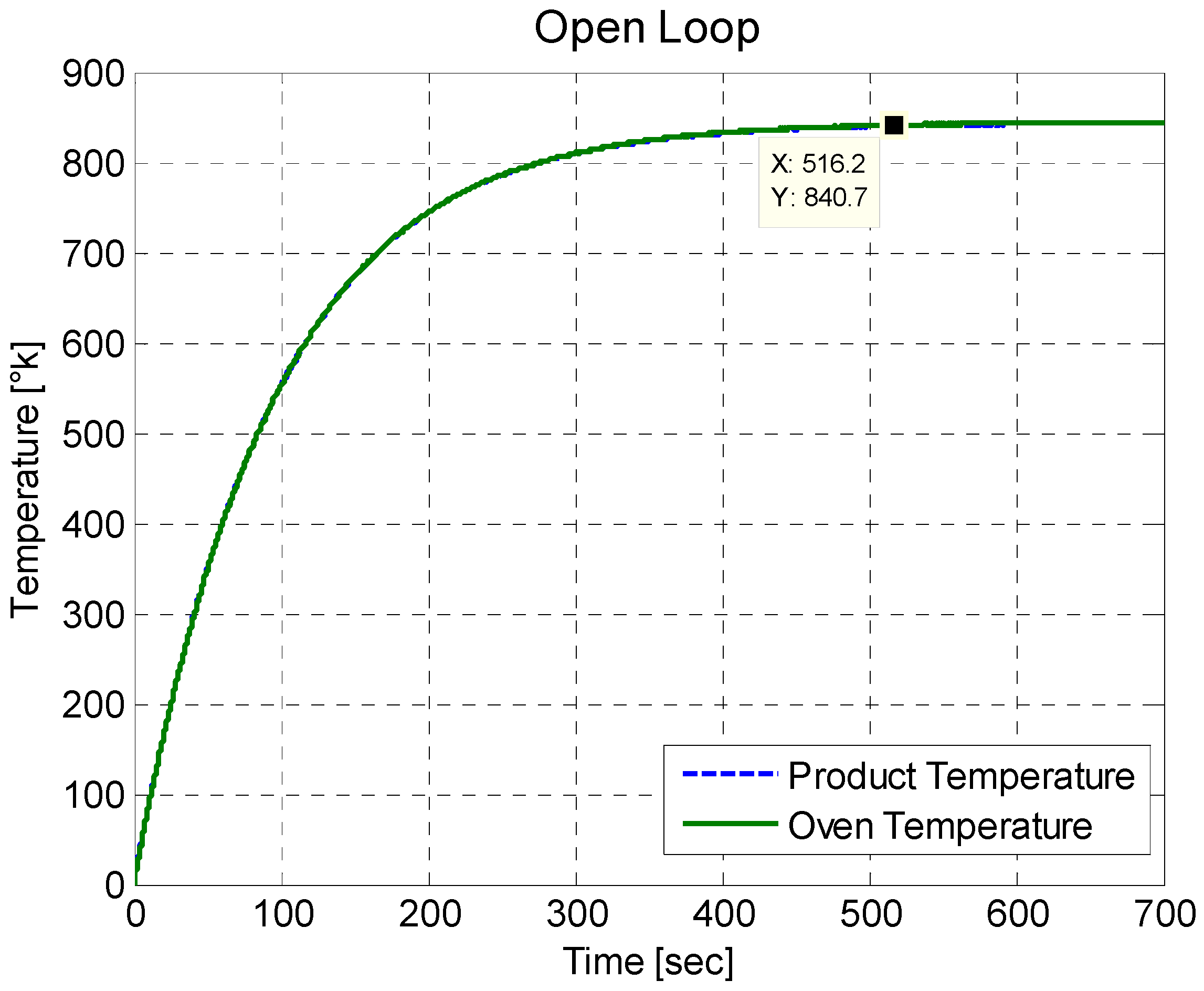
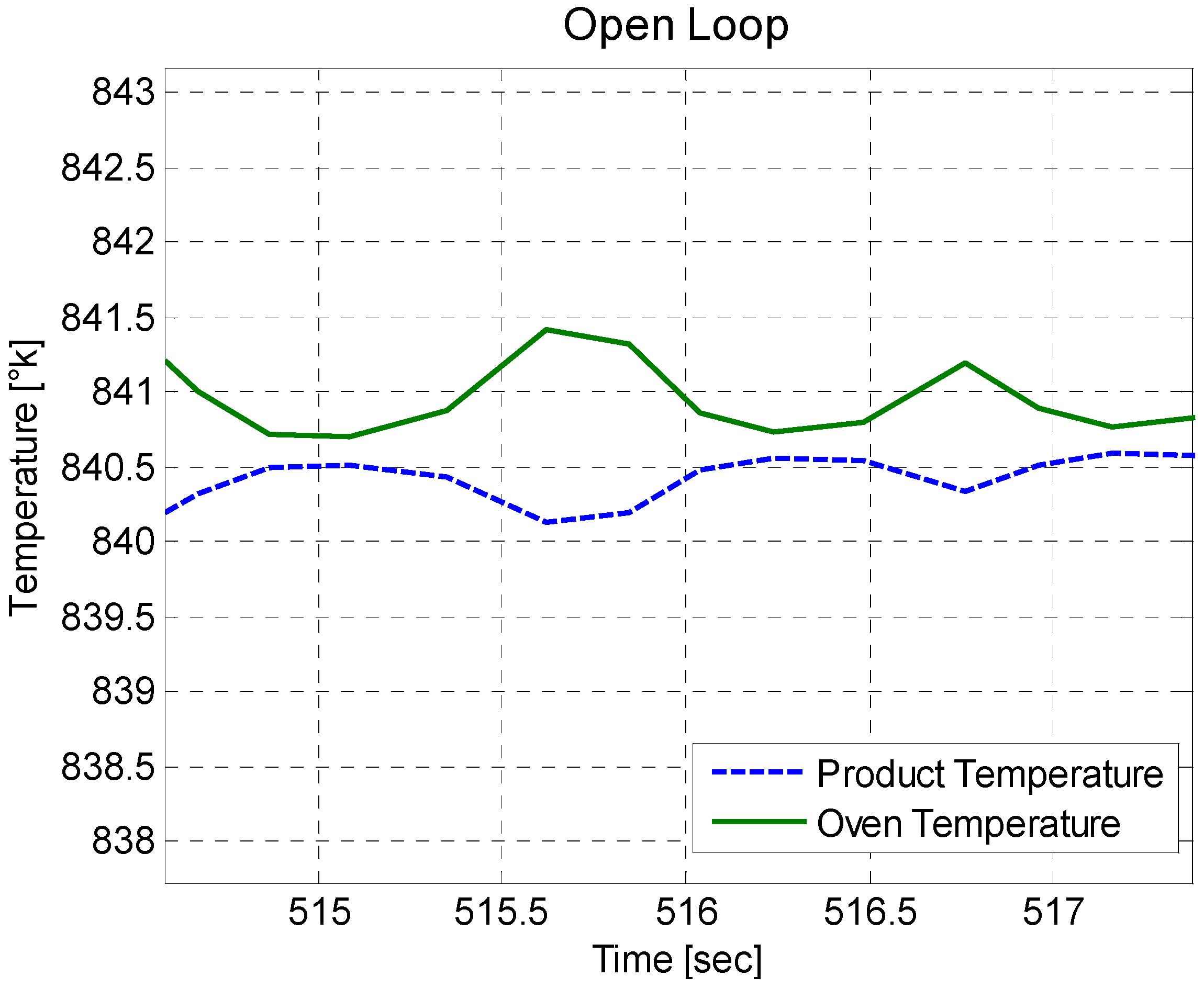
Figure 4 shows the behavior of the electric oven leading to a maximum temperature of $840.7\mathrm{K}$.The simulated oven temperatures, with respect to the simulated product temperatures, are very similar, as can be seen in Figure 5, which is a zoom of Figure 4.

It can also be seen in Figure 4 that the growth in temperature of the electric furnace takes a long convergence time to reach its limit temperature. This limit temperature is due to the heat capacitance of the furnace—to reach the limit temperature more quickly, it would need to be increased with an amount of power supplied greater than 127 VA. Figure 4 and Figure 5 are obtained using Equation (4).

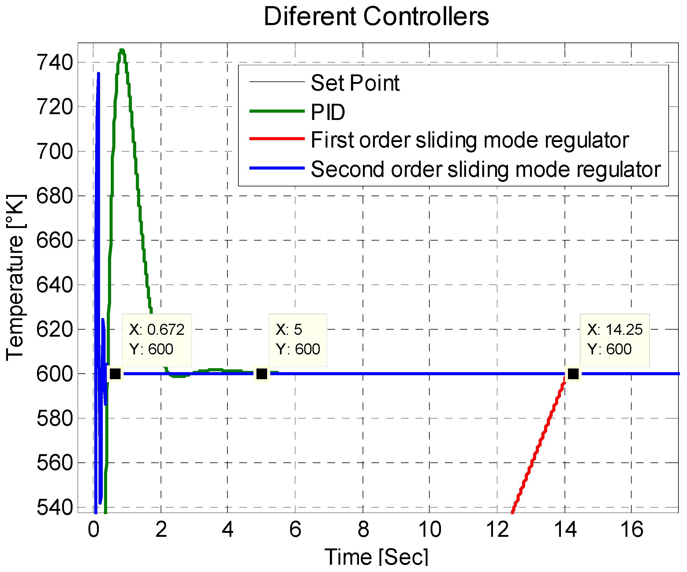
The response of the electric oven corresponds to a stable linear mathematical model; however, it has a regulator at a desired temperature, and this is maintained in that range. The PID regulator and the two sliding-mode regulators can be seen in Figure 6. For this mathematical model all regulators reach the set point; however, the difference is in the convergence time. For the first-order sliding-mode regulator, its convergence time is 14.25 s. For the PID regulator, its convergence time is 5 s. For the second-order sliding-mode regulator, its convergence time is 0.672 s, having a much faster convergence time than the other two regulators, and avoiding the chattering of the first-order sliding-mode regulator. Figure 7 is a zoom of Figure 6 to visualize the convergence times of the regulators that are applied to the electric oven. Equations (7) and (13), in a feedback model with a reference value of 600, correspond to Figure 6 and Figure 7, for the PID regulator. For the first-order sliding-mode regulator, Equations (7) and (15), in the same way, in a feedback model with a reference value of 600 can be seen in Figure 6 and Figure 7. In a very similar way, Equations (7) and (20) correspond to the response of Figure 6 and Figure 7 for the second-order sliding-mode regulator.

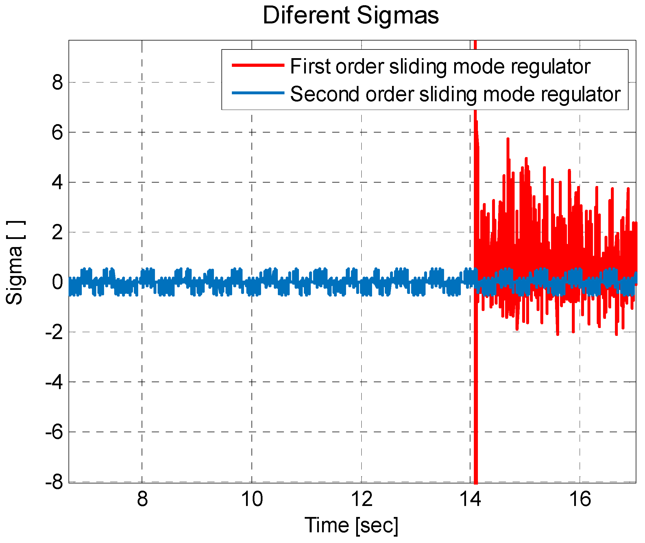
Another important point to check is the value of $\sigma ,$ also known as the hyperplane, where $\sigma \to 0$; this $\sigma$ refers to the first-order sliding-mode regulator and the second-order sliding-mode regulator. This result can be seen in Figure 8, where the sigma value for the second-order sliding-mode regulator tends to reach a value closer to zero, and in a shorter convergence time.

5.2. Simulation Results for the Inverted Pendulum

In this subsection, the mathematical model of the inverted pendulum is used, to which three regulators are applied—a PID regulator, a first-order sliding-mode regulator, and a second-order sliding-mode regulator. The mathematical model is important in this subsection, since, by nature, the inverted pendulum tends to be at an unwanted point of rest, which greatly complicates the performance of the regulators, and highlights the advantages and disadvantages of each regulator.

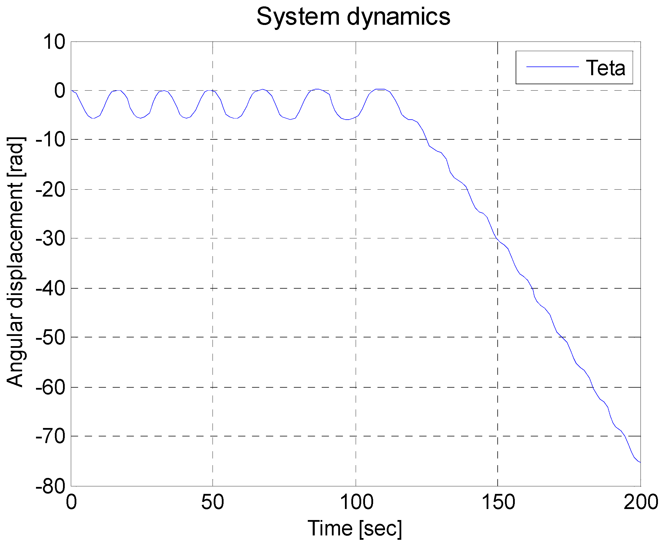
It is important to know the behavior of the inverted pendulum by applying an external force which generates a displacement, and, in turn, an angular movement at the joint of the pendulum bar and the cart. In Figure 9, the output response can be seen—it is interesting to note the type of response, since in the first 100 s, the angular displacement keeps oscillating and later the mathematical model becomes unstable—this indicates that the force is enough to rotate the pendulum bar in one direction. This is because in the mathematical model of the inverted pendulum, the coefficients of friction in the vehicle wheels, the pendulum rod, and the car are not considered. For these reasons, this is an asymmetrical unstable non-linear mathematical model, making it difficult to obtain a regulator with an acceptable performance.

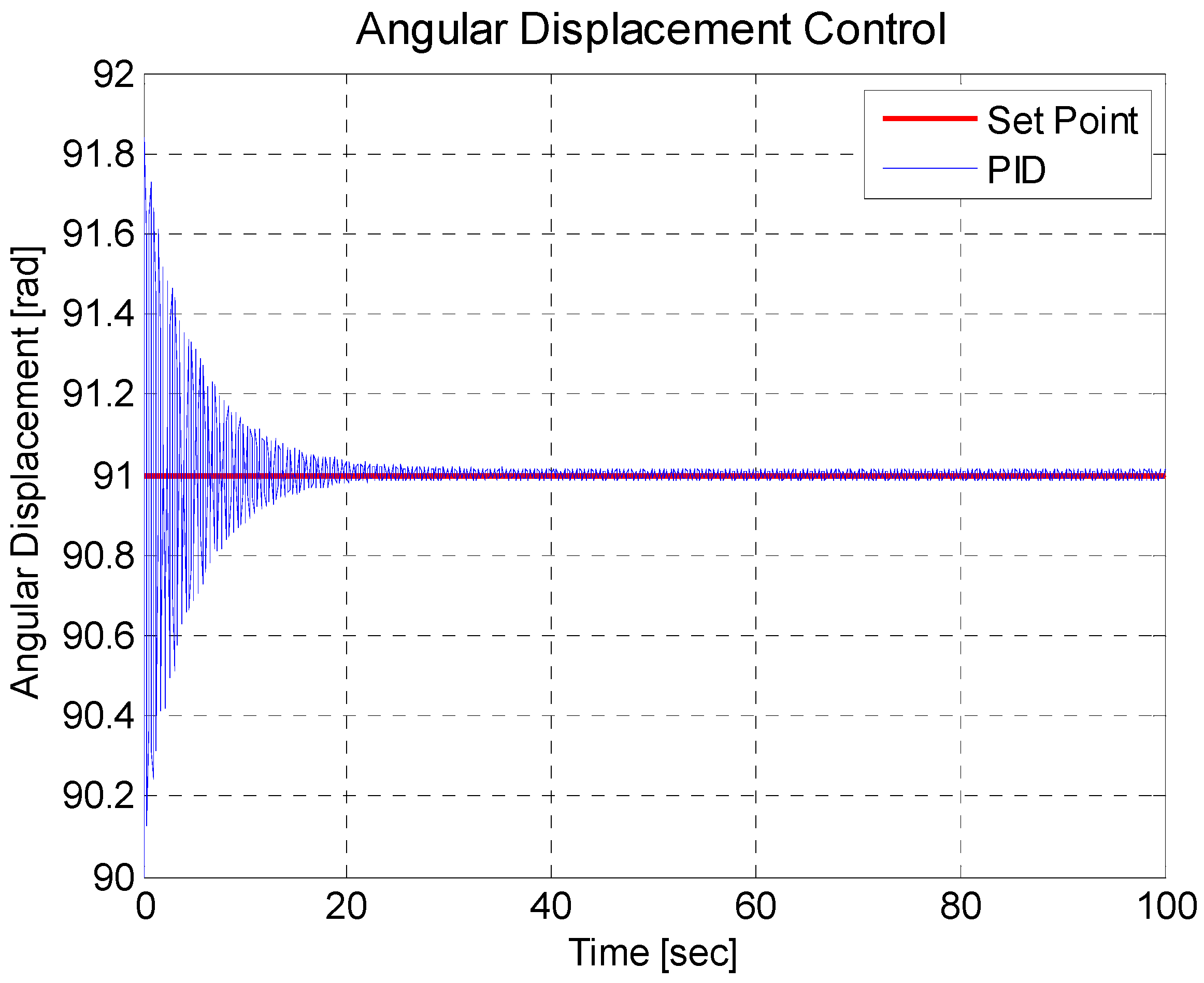
For the development of the regulator, the idea is that the inverted pendulum bar takes a positive vertical position, where, to help the inverted pendulum behavior, it will be considered to place an initial condition, which is to place the bar at 90° or $\left(\frac{\pi }{2}\right)$. The responses of the PID regulator are seen in Figure 10, where the regulator, in a very general way, reaches the set point, since it generates oscillations, which gradually decrease until the oscillations are very close to the set point.

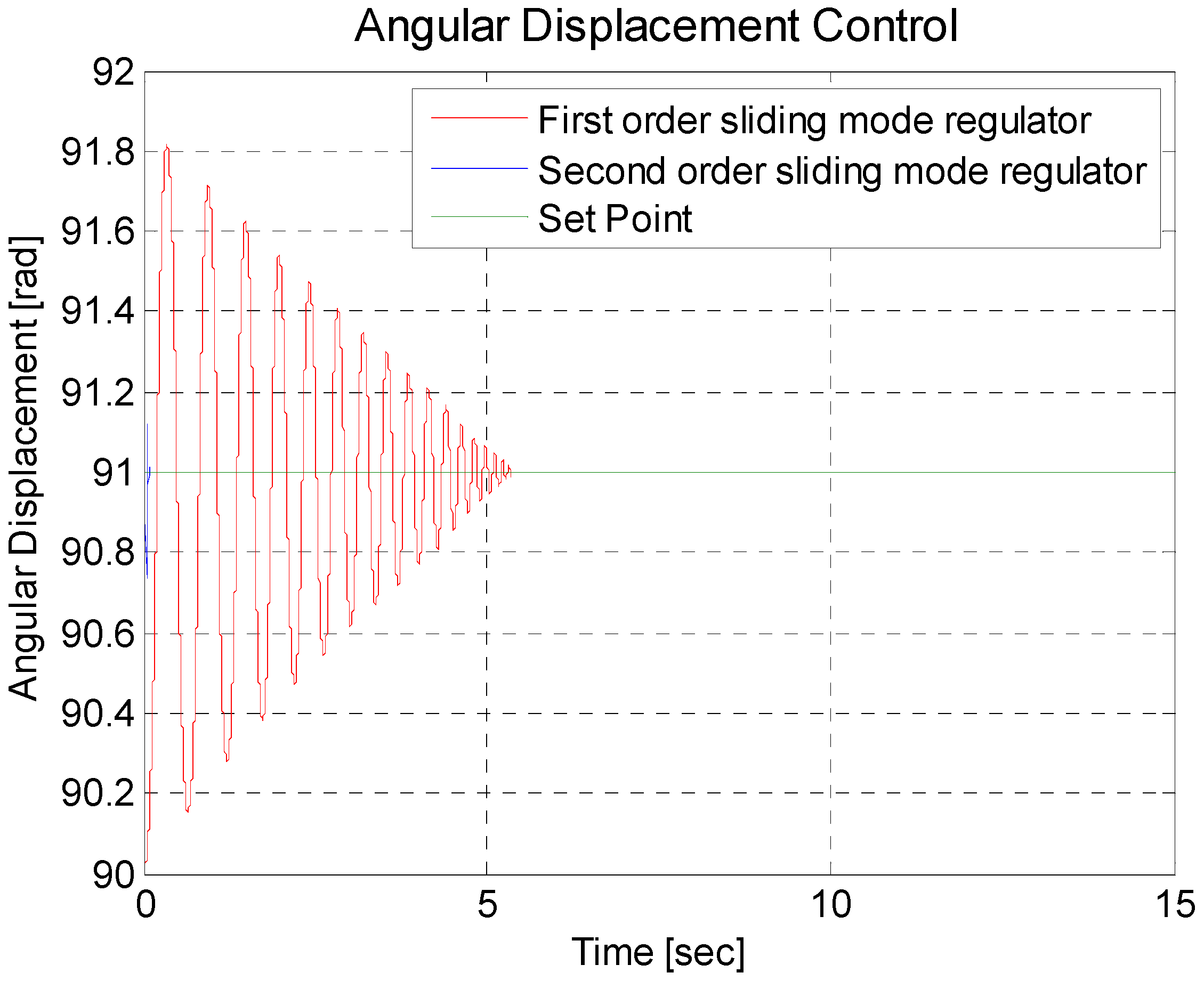
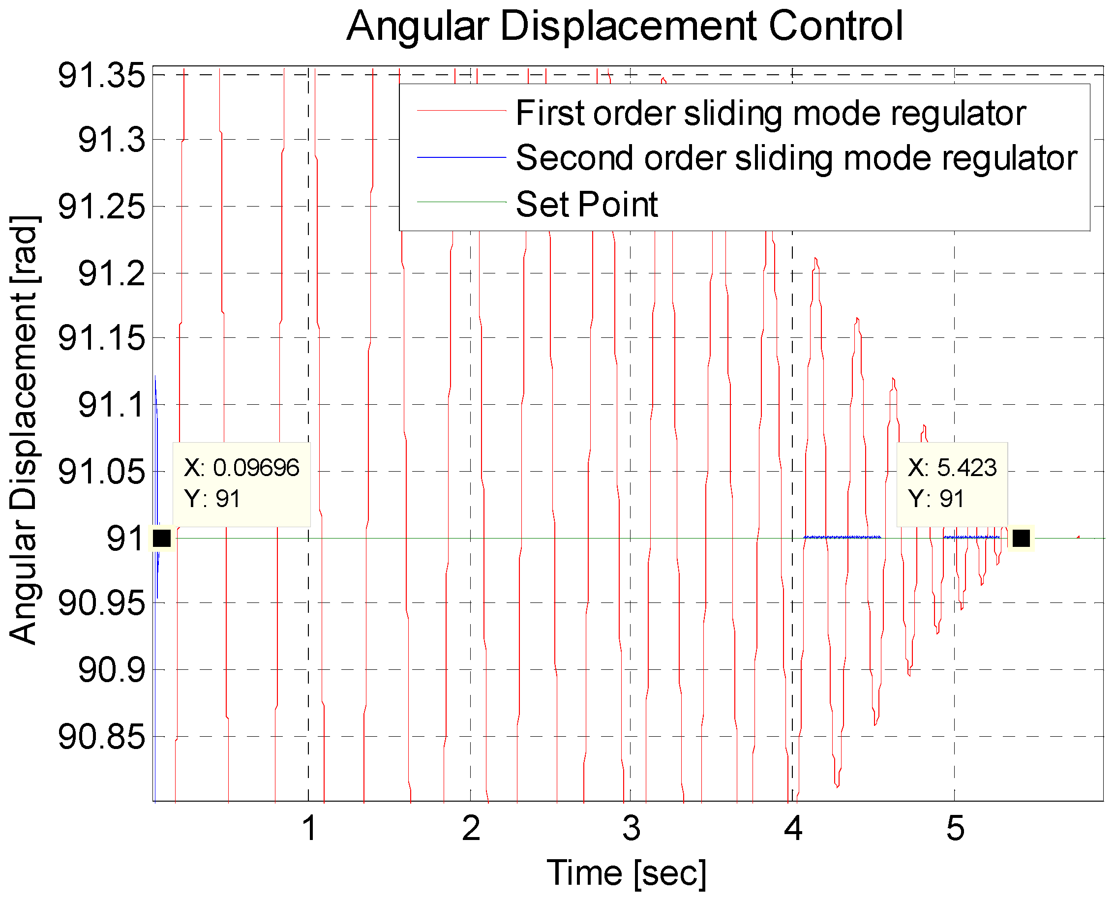
For the two sliding-mode regulators, in Figure 11, it can be seen that both regulators reach the set point; the difference between them is the convergence time, which can be seen more clearly in Figure 12. The second-order sliding regulator has a convergence time of approximately 0.1 s, and the first-order sliding-mode regulator has a convergence time of 5.4 s. Figure 12 is a zoom of Figure 11, to visualize the convergence times of the regulators that are applied to the inverted pendulum. Equations (8) and (34) and Equations (8) and (38), in a feedback model with a reference value of 91, correspond to the first-order sliding-mode regulator and the second-order sliding-mode regulator of Figure 11 and Figure 12.

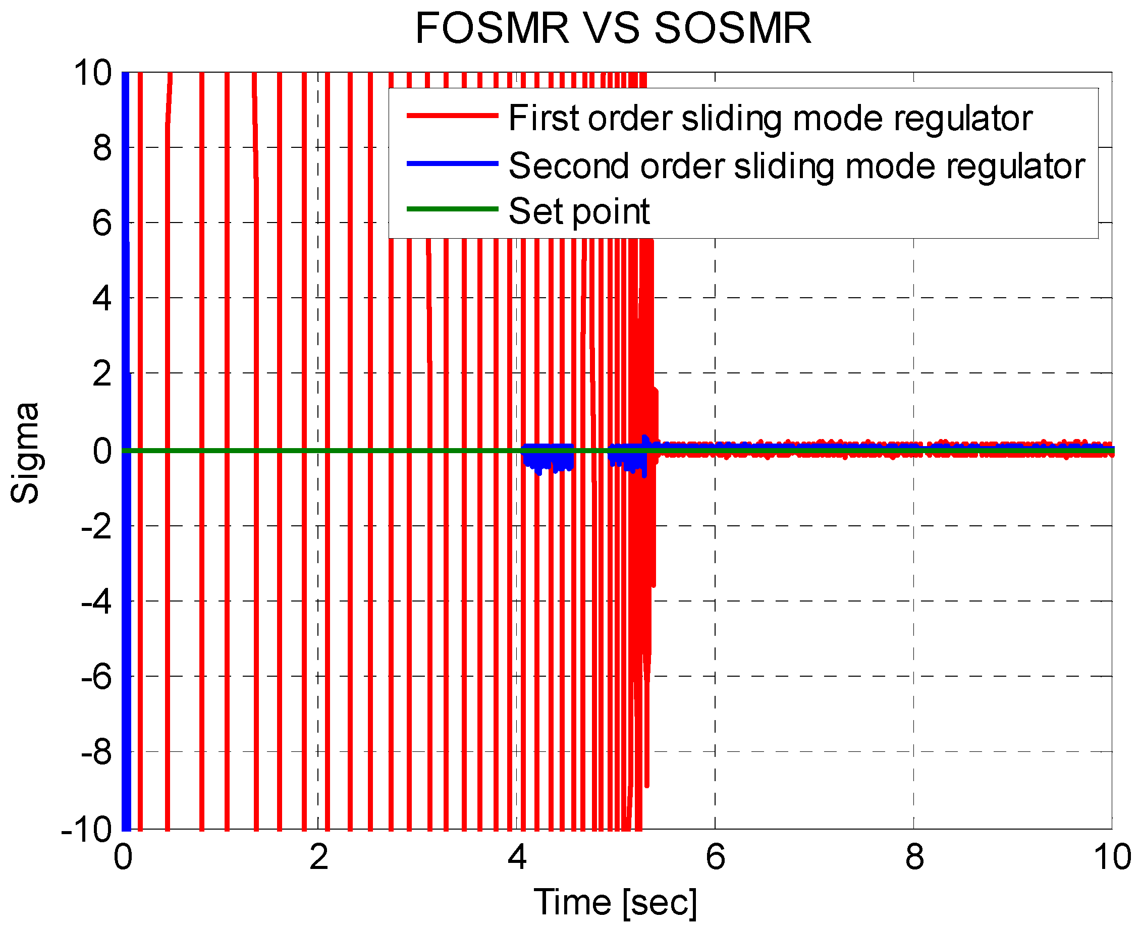
It is also necessary to consider the behavior of $\sigma$, where its convergence must reach zero. This behavior is seen in Figure 13, where the sigma function of the second-order sliding-mode regulator is closer to zero, in addition to achieving this in a shorter convergence time. Figure 13 is a zoom to more clearly show $\sigma$ for the two sliding-mode regulators.

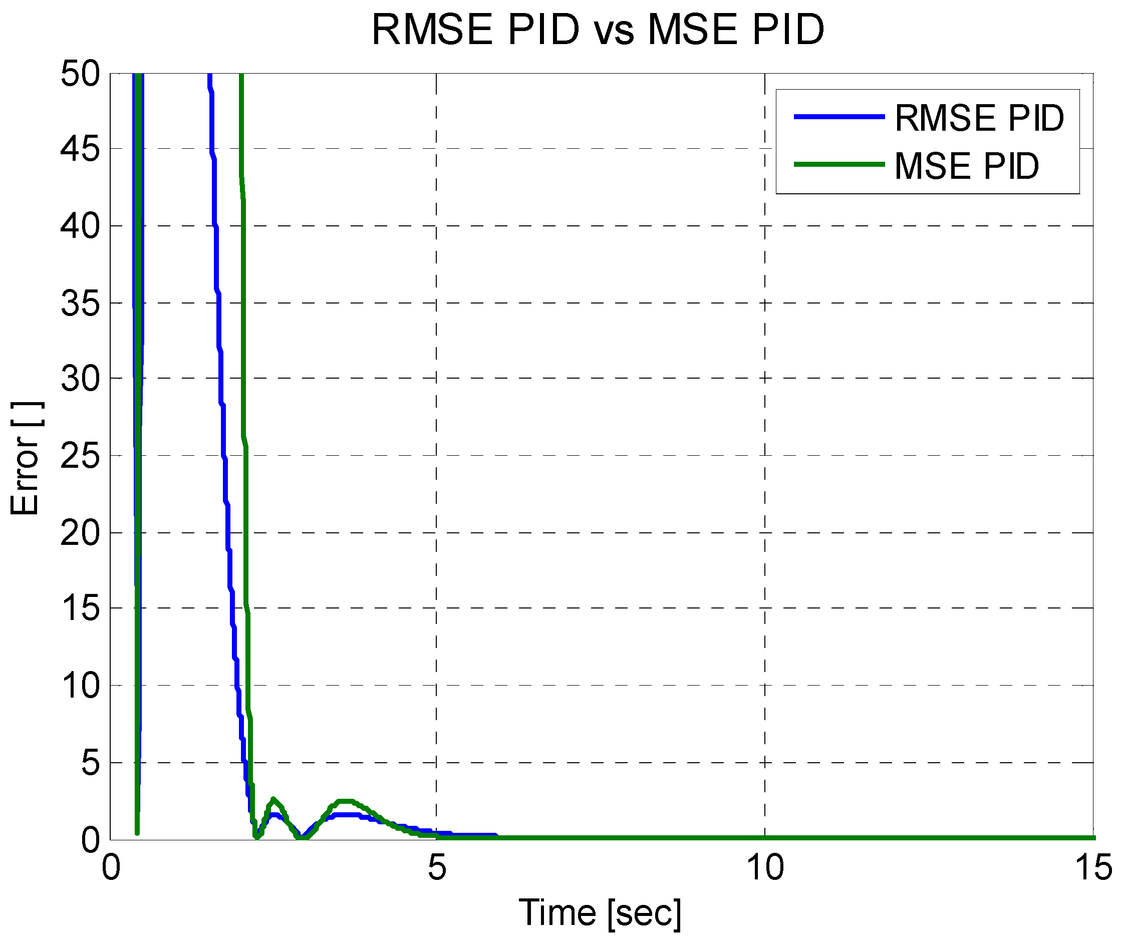
5.3. Simulation Results of the Electric Oven Errors

In this subsection, an analysis of the errors of each of the regulators is presented for the electric oven—three types of regulators are used: the PID regulator, the first-order sliding-mode regulator, and the second-order sliding-mode regulator. The types of errors arising are represented by Equations (41) and (42), where $e=r-y$ is the error, $r$ is the set point, $y$ is the output, and T is the period in which it will be evaluated.

$$\mathrm{MSE}=\frac{1}{T}{{\displaystyle \int }}_0^T{\left(e\right)}^{2}dt$$

(41)

$$\mathrm{RMSE}=\sqrt{\frac{1}{T}{{\displaystyle \int }}_0^T{\left(e\right)}^{2}dt}$$

(42)

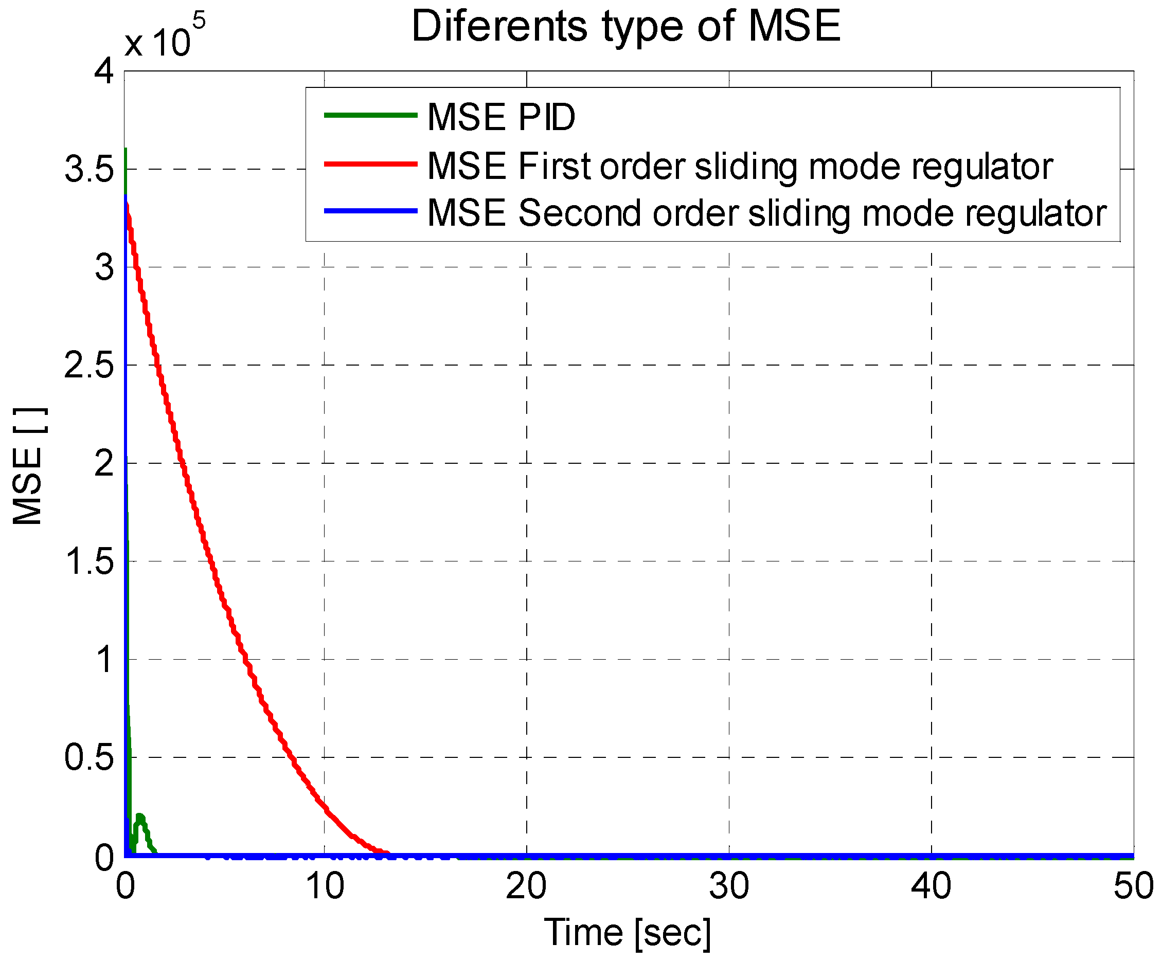
Figure 14 shows a zoom of the behavior of the two types of error in order to more clearly see their behaviors. The mean square error of Equation (41), and the root mean square error of Equation (42), are derived, where it is seen that both reach the value of zero. On the other hand, Figure 15 shows a comparison of the mean square error for the three types of regulators, where these reach the value of zero, indicating the proper functioning of the regulators. However, the idea is to analyze which regulator has the best performance for this. The average is calculated for the mean square error and the root mean square error; these results can be seen in

Table 3. Regulator errors for electric oven.

Type of Regulator	MSE	RMSE
PID	0.302360209	0.074114764
First-order sliding-mode	15620.04074	51.3949548
Second-order sliding-mode	5.49191 × 10−8	0.000146729

.

In Table 3, it is shown that the regulator with the best performance is the second-order sliding-mode regulator; this is due to the convergence time with which it responds, since it is one of the characteristics of this type of regulator.

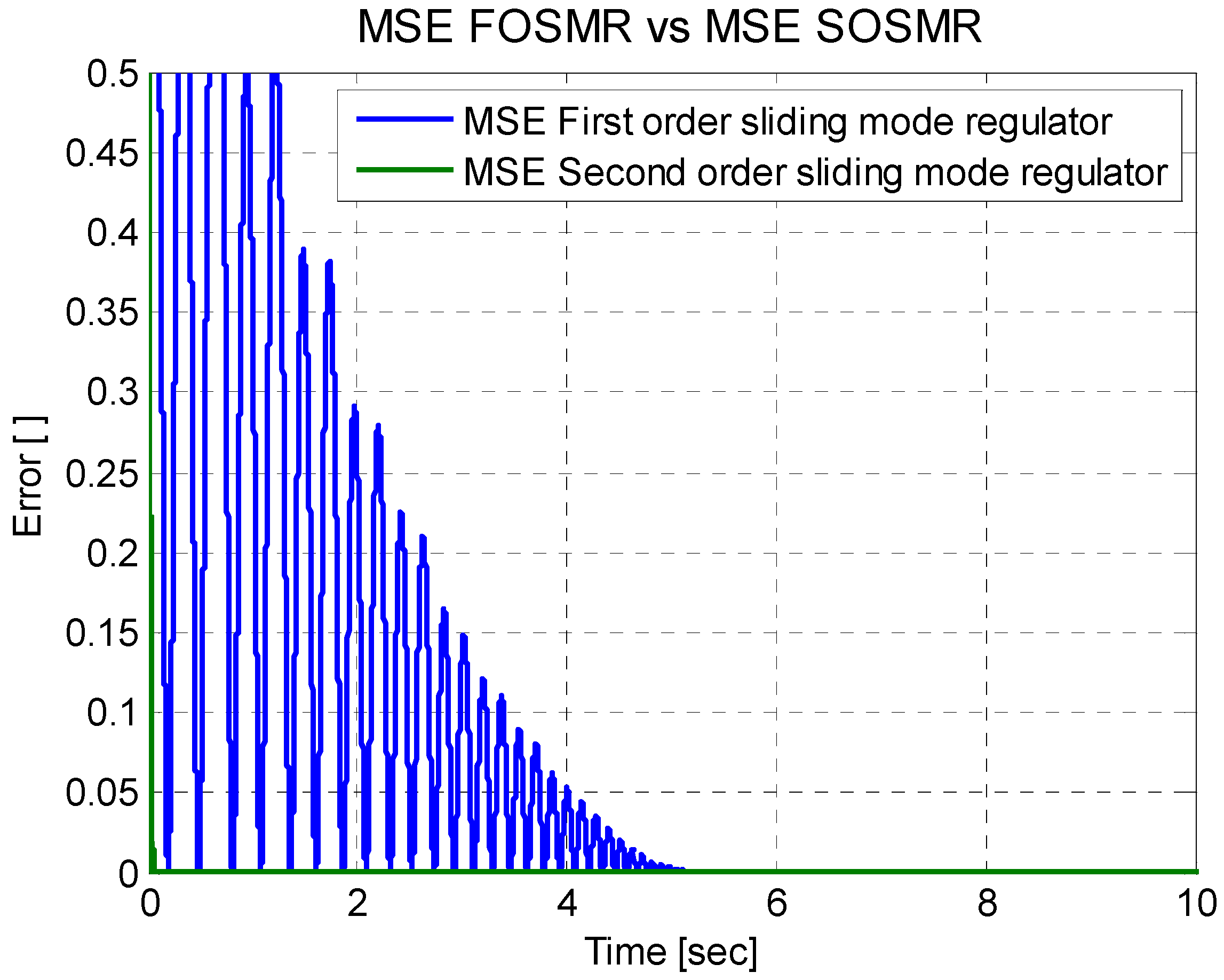
5.4. Simulation Results of the Inverted Pendulum Errors

In this subsection, an analysis of the errors for the regulators is presented for the inverted pendulum.

In Figure 16, a graph of two types of errors is presented showing the mean square error of Equation (37) and the root mean square error of Equation (38), which assists in evaluating how efficient a regulator is. For this, an average of these errors is also calculated using Equations (37) and (38); these values can be seen in

Table 4. Regulator errors for inverted pendulum.

Type of Regulator	MSE	RMSE
PID	0.306299034	0.155970195
First-order sliding-mode	0.158	0.264
Second-order sliding-mode	0.000676	0.000854

.

Figure 17 shows the mean square error of the sliding-mode regulator with respect to the second-order sliding-mode regulator, where it is noted that the second-order sliding-mode regulator has a better performance; the identified errors are detailed in Table 4. The regulator with the best performance is the second-order sliding-mode regulator, since this regulator has an error which is closer to zero.

In Table 4, it is clearly seen that the second-order sliding-mode regulator has a smaller average error, both for the mean square error and for the root mean square error. This can also be seen in the simulation graphs.

6. Experimental Results

This section considers the experimental comparison between the mathematical model and the real data model, which is applied to two mathematical models; the first is an electric oven and the second is an inverted pendulum. For these comparisons, Matlab was used to represent the results. The real data model was obtained using an electronic target and communication with Matlab.

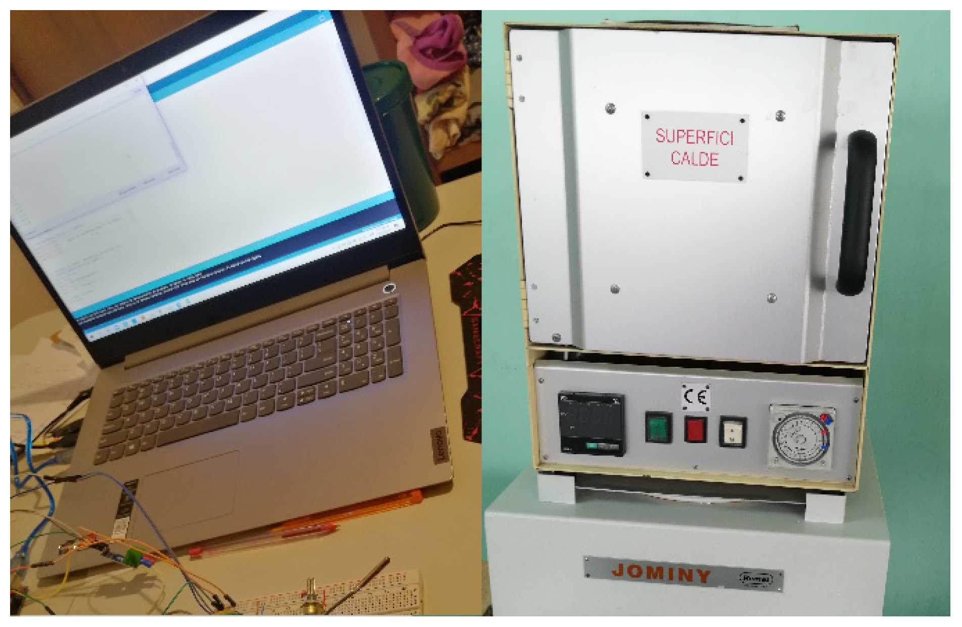
6.1. Experimental Results of the Electric Oven

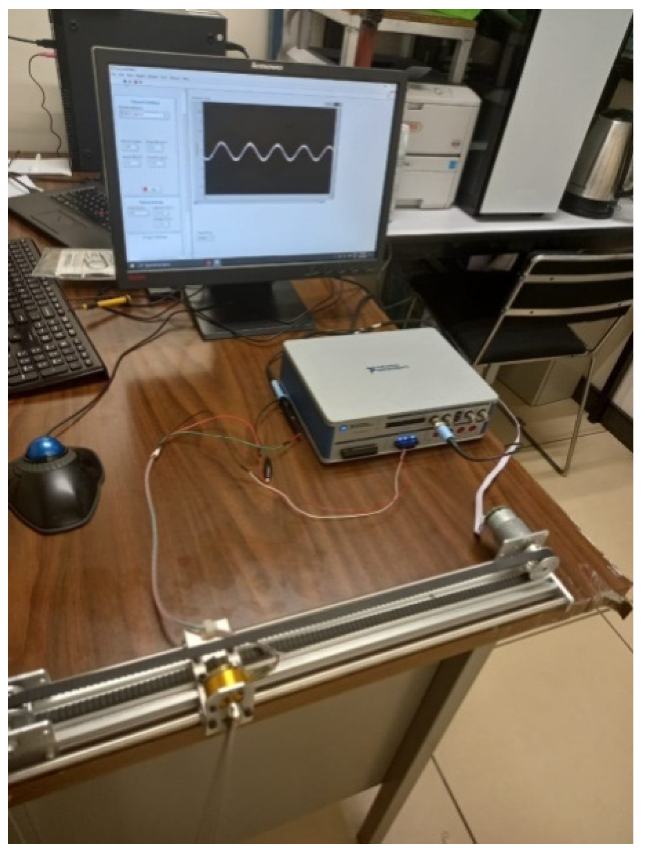
This subsection focuses on the comparison between the mathematical model and the real data model. The data acquisition for the real data model was obtained from the electric oven of Figure 18 (this is seen on the right side). On the left side, the interface of a program for the data acquisition is shown. The electric furnace was located in the Materials Laboratory of the Postgraduate Section of the ESIME Azcapotzalco, National Polytechnic Institute in Mexico.

One of the problems in the data acquisition was that the regulator of the electric oven did not reach the reference value to which it was programmed. In addition, the response speed of the regulator was slow. To solve these problems, the proposed regulators for the electric oven were used instead of the conventional regulators. To do this, the following steps were considered: the first step was to perform a study of the behavior of the electric oven; this was achieved using the Fourier equations for temperature behavior. In the second step, the data acquisition for the electric oven was obtained using the electronic target and the electronic instrumentation; the real data provided an output response of the oven temperature.

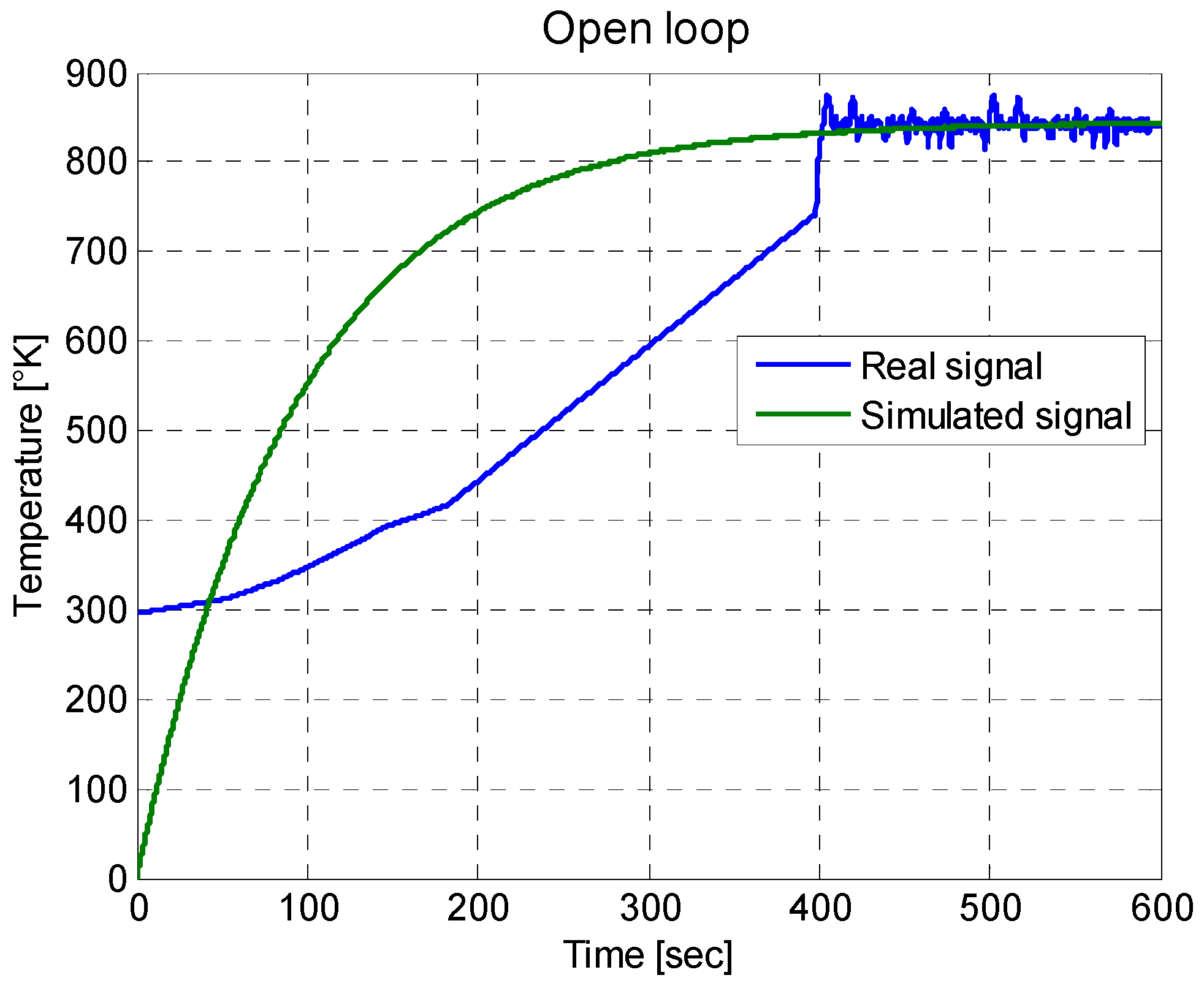
As there is a mathematical model and a real data model, a comparison can be made between both models. This comparison was made using Matlab. In Figure 19, it can be seen that, for the behavior of the simulated signal (in green) and the behavior of the real signal (in blue), there was a difference for the first 400 s—after that, both models were similar. The difference was because the real data model started at a temperature of 300 °K or 27 °C, while in the mathematical model this initial condition was not considered.

6.2. Experimental Results of the Inverted Pendulum

In this subsection, the experiments of the inverted pendulum are analyzed, and the comparison between the real data model and the mathematical model is presented. The data acquisition for the real data model was obtained from the inverted pendulum of Figure 20.

In this experiment, one of the problems was that the movement of the car was through a toothed band which provided a different friction coefficient than had it been in a smooth band; this friction coefficient is not considered in the mathematical model as this could generate a small difference between the regulators.

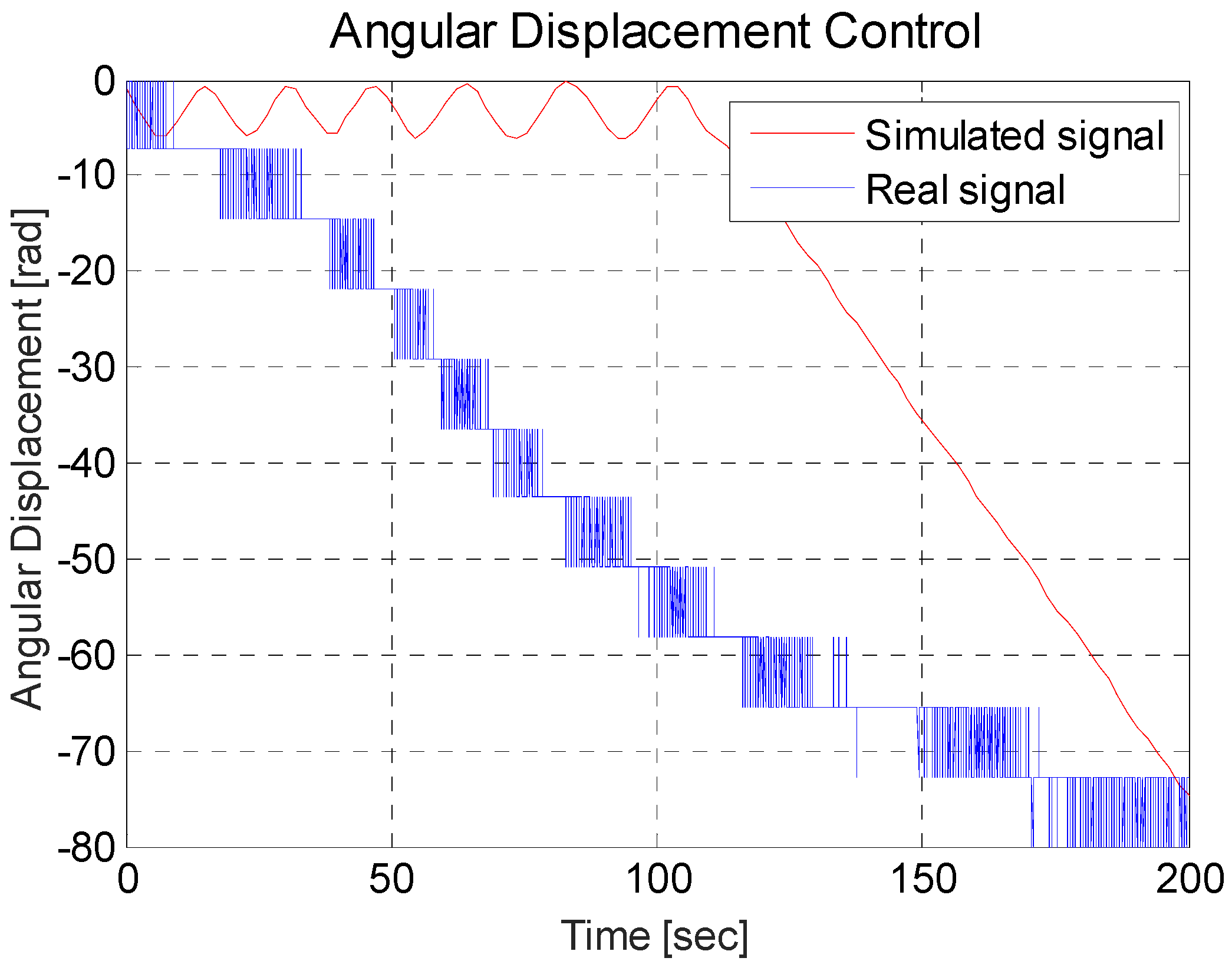
The encoder and the coupling of the bar of the encoder also yielded a friction coefficient which showed a small difference between the real data model and the mathematical model; this can be seen in Figure 21. It is possible to see that the real signal began to decrease its oscillations faster than the simulated signal; however, the behavior of the mathematical model and real data model were very similar since both signals generated oscillations, and after a convergence time the oscillations decreased.

Remark 3.

In this section, the experimental comparisons between the real signal and simulated signal for the electric oven and inverted pendulum are presented to show that the mathematical models were similar to the real data models.

Remark 4.

For the experiments, linear mathematical models were considered because linearization allows the transfer functions to be obtained, the transfer functions allow the application of the z-transform, and the z-transform allows use of the Arduino platform for application of the regulators in discrete time [15,16]. It is necessary to add the analog inputs of the sensors to obtain a PWM signal which is sent to the electric power regulator; the inputs are stored within a program. Within the Arduino platform, the equations of the regulators are placed in discrete time where a sampling time of 8 sec is enabled; the gains are already calculated and are added in the program.

Remark 5.

One of the drawbacks is the integral component of the PID regulator and the second-order sliding-mode regulator; this is because it consumes too much processing when performing the calculations. Small gains in the integral part of the regulators decrease this drawback. The second-order sliding-mode regulator improves the PID regulator because the second-order sliding-mode regulator uses smaller gains than the PID regulator.

7. Conclusions

The PID regulator is well-known in the literature—a proposed regulator must have better characteristics than the PID regulator. Thus, the PID regulator was compared with a first-order sliding-mode regulator, and a second-order sliding-mode regulator to consider two outcomes: (1) one outcome considered was to see if there is a regulator that can replace the PID regulator; for this comparison, an electric oven was considered as a stable linear mathematical model, and an inverted pendulum was considered as an asymmetric unstable non-linear mathematical model. In both cases, the two sliding-mode regulators reached the set point; this did not happen with the PID regulator which kept oscillating around the set point in the inverted pendulum; (2) Another outcome considered was how to reduce chattering when applying the sliding-mode regulators; this reduction in chattering was achieved using the second-order sliding-mode regulator, but was not achieved using the first-order sliding-mode regulator. A limitation of the proposed regulator is that convergence of the second sliding-mode regulator was not demonstrated; further investigations to address this limitation will be considered as part of future research. Finally, the experimental comparisons between the real signal and simulated signal for the electric oven and inverted pendulum were presented, showing that the mathematical models were similar to the real data models. In the future, the studied regulators will be compared with other strategies, such as the H-2 or H-infinity, the second-order sliding-mode regulator will be implemented, and the over/undershoots and disturbances will be assessed.

References

- Huba, M.; Chamraz, S.; Bistak, P.; Vrancic, D. Making the PIand PID Controller Tuning Inspired by Ziegler and Nichols Precise and Reliable. Sensors 2021, 21, 6157. [Google Scholar] [CrossRef] [PubMed]
- Vrancic, D.; Huba, M. High-Order Filtered PID Controller Tuning Based on Magnitude Optimum. Mathematics 2021, 9, 1340. [Google Scholar] [CrossRef]
- Huba, M.; Vrancic, D. Extending the Model-Based Controller Design to Higher-Order Plant Models and Measurement Noise. Symmetry 2021, 13, 798. [Google Scholar] [CrossRef]
- Huba, M.; Bistak, P.; Vrancic, D.; Zakova, K. Dead-Time Compensation for the First-Order Dead-Time Processes: Towards a Broader Overview. Mathematics 2021, 9, 1519. [Google Scholar] [CrossRef]
- Huba, M.; Oliveira, P.M.; Bistak, P.; Vrancic, D.; Zakova, K. A Set of Active Disturbance Rejection Controllers Based on Integrator Plus Dead-Time Models. Appl. Sci. 2021, 11, 1671. [Google Scholar] [CrossRef]
- De Moura Oliveira, P.B.; Hedengren, J.D.; Solteiro Pires, E.J. Swarm-Based Design of Proportional Integral and Derivative Controllers Using a Compromise Cost Function: An Arduino Temperature Laboratory Case Study. Algorithms 2020, 13, 315. [Google Scholar] [CrossRef]
- Rouabah, B.; Toubakh, H.; Sayed-Mouchaweh, M. Fault tolerant control of multicellular converter used in shunt active power filter. Electr. PowerSyst. Res. 2020, 188, 106533. [Google Scholar] [CrossRef]
- Aravindh, D.; Sakthivel, R.; Kong, F.; Marshal Anthoni, S. Finite-time reliable stabilization of uncertain semi-Markovian jump systems with input saturation. Appl. Math. Comput. 2020, 384, 125388. [Google Scholar] [CrossRef]
- Song, S.; Zhang, B.; Xia, J.; Zhang, Z. Adaptive Backstepping Hybrid Fuzzy Sliding Mode Control for Uncertain Fractional-Order Nonlinear Systems Based on Finite-Time Scheme. IEEE Trans. Syst. Man Cybern. Syst. 2020, 50, 1559–1569. [Google Scholar] [CrossRef]
- Song, S.; Zhang, B.; Song, X.; Zhang, Y.; Zhang, Z.; Li, W. Fractional-order adaptive neuro-fuzzy sliding mode H∞ control for fuzzy singularly perturbed systems. J. Frankl. Inst. 2019, 356, 5027–5048. [Google Scholar] [CrossRef]
- Yu, L.; Huang, J.; Fei, S. Robust Switching Control of the Direct-Drive Servo Control Systems Based on Disturbance Observer for Switching Gain Reduction. IEEE Trans. Circuits Syst.-II Express Briefs 2019, 66, 1366–1370. [Google Scholar] [CrossRef]
- Fu, H.; Li, J.; Han, F.; Hou, N.; Dong, H. Outlier-resistant observer-based H-infinity PID control under stochastic communication protocol. Appl. Math. Comput. 2021, 411, 126535. [Google Scholar]
- Peng, J.; Yang, Z.; Wang, Y.; Zhang, F.; Liu, Y. Robust adaptive motion/force control scheme for crawler-type mobile manipulator with nonholonomic constraint based on sliding mode control approach. ISA Trans. 2019, 92, 166–179. [Google Scholar] [CrossRef]
- Zhi, J.; Chen, Y.; Dong, X.; Liu, Z.; Shi, C. Robust adaptive FTC allocation for overactuated systems with uncertainties and unknown actuator non-linearity. IET Control Theory Appl. 2018, 12, 273–281. [Google Scholar] [CrossRef]
- Jäntschi, L. The Eigenproblem Translated for Alignment of Molecules. Symmetry 2019, 11, 1027. [Google Scholar] [CrossRef] [Green Version]
- Joita, D.-M.; Tomescu, M.A.; Balint, D.; Jäntschi, L. An Application of the Eigenproblem for Biochemical Similarity. Symmetry 2021, 13, 1849. [Google Scholar] [CrossRef]
- Sharma, J.R.; Kumar, S.; Jäntschi, L. On a Class of Optimal Fourth Order Multiple Root Solvers without Using Derivatives. Symmetry 2019, 11, 1452. [Google Scholar] [CrossRef] [Green Version]
- Truskey, G.; Yuan, F.; Katz, D. Transport Phenomena in Biological Systems, 2nd ed.; Pearson Prentice Hall: Atlanta, GA, USA, 2010; ISBN -10:0131569880. [Google Scholar]
- Bajrami, X.; Pajaziti, A.; Likaj, R.; Shala, A.; Berisha, R.; Bruqi, M. Control Theory Application for Swing Up and Stabilisation of Rotating Inverted Pendulum. Symmetry 2021, 13, 1491. [Google Scholar] [CrossRef]
- Estevez, J.; Lopez-Guede, J.M.; Garate, G.; Graña, M. A Hybrid Control Approach for the Swing Free Transportation of a Double Pendulum with a Quadrotor. Appl. Sci. 2021, 11, 5487. [Google Scholar] [CrossRef]
- Kong, F. Subharmonic Solutions with Prescribed Minimal Period of a Forced Pendulum Equation with Impulses. Acta Appl. Math. 2018, 158, 125–137. [Google Scholar] [CrossRef]
- Rahmani, R.; Mobayen, S.; Fekih, A.; Ro, J.-S. Robust Passivity Cascade Technique-Based Control Using RBFN Approximators for the Stabilization of a Cart Inverted Pendulum. Mathematics 2021, 9, 1229. [Google Scholar] [CrossRef]
- Feng, Z.; Li, S.; Ahn, C.K.; Xiang, Z. On the Finite-Time Stabilization for a Class of Interconnected Switched Nonlinear Systems via Sampled-Data Output Feedback Control. IEEE Syst. J. 2021. [Google Scholar] [CrossRef]
- Fantoni, I.; Lozano, R. Non-Linear Control for Underactuated Mechanical Systems, 1st ed.; Springer: London, UK, 2002; ISBN 978-1-4471-1086-6. [Google Scholar]
Figure 1.
Free-body diagram of an electric oven.
Figure 2.
Free-body diagram of the inverted pendulum.
Figure 4.
Behavior of the electric oven.
Figure 5.
Zoom of the behavior of the oven temperature with respect to the simulated product temperature.
Figure 6.
PID regulator and two sliding-mode regulators.
Figure 7.
Zoom of the three regulators to see the convergence time with the set point.
Figure 8.
Different sigma responses.
Figure 9.
Open loop mathematical model of the inverted pendulum.
Figure 10.
Inverted pendulum response with PID regulator.
Figure 11.
Response of the inverted pendulum by two sliding-mode regulators.
Figure 12.
Zoom of two sliding-mode regulators to see the convergence time with the set point for the inverted pendulum.
Figure 13.
Zoom of the sigma for two sliding-mode regulators.
Figure 14.
Zoom of the root mean square error and mean square error.
Figure 15.
MSE for three types of regulator.
Figure 16.
Root mean square error and mean square error.
Figure 17.
Root mean square error of regulators with sliding-mode.
Figure 18.
The data acquisition of the electric oven.
Figure 19.
Comparison between a real signal and a simulated signal for the electric oven.
Figure 20.
The data acquisition of the inverted pendulum.
Figure 21.
Comparison between the real signal and simulated signal for the inverted pendulum.